Unsupervised Machine Learning and Data Mining Procedures Reveal Short Term, Climate Driven Patterns Linking Physico-Chemical Features and Zooplankton Diversity in Small Ponds

Abstract

Machine Learning (ML) is an increasingly accessible discipline in computer science that develops dynamic algorithms capable of data-driven decisions and whose use in ecology is growing. Fuzzy sets are suitable descriptors of ecological communities as compared to other standard algorithms and allow the description of decisions that include elements of uncertainty and vagueness. However, fuzzy sets are scarcely applied in ecology. In this work, an unsupervised machine learning algorithm, fuzzy c-means and association rules mining were applied to assess the factors influencing the assemblage composition and distribution patterns of 12 zooplankton taxa in 24 shallow ponds in northern Italy. The fuzzy c-means algorithm was implemented to classify the ponds in terms of taxa they support, and to identify the influence of chemical and physical environmental features on the assemblage patterns. Data retrieved during 2014 and 2015 were compared, taking into account that 2014 late spring and summer air temperatures were much lower than historical records, whereas 2015 mean monthly air temperatures were much warmer than historical averages. In both years, fuzzy c-means show a strong clustering of ponds in two groups, contrasting sites characterized by different physico-chemical and biological features. Climatic anomalies, affecting the temperature regime, together with the main water supply to shallow ponds (e.g., surface runoff vs. groundwater) represent disturbance factors producing large interannual differences in the chemistry, biology and short-term dynamic of small aquatic ecosystems. Unsupervised machine learning algorithms and fuzzy sets may help in catching such apparently erratic differences.

1. Introduction

Data in ecology often present high stochasticity, correlated features and a large number of predictors compared to the sample size of the dataset. In community analysis, useful techniques to explore environmental and biological datasets include multivariate analyses and classical clustering algorithms. The rise of machine learning algorithms in ecology in recent decades has become accessible thanks to the advance in computation power, large amounts of data and software availability [1]. These algorithms are well suited to deal with complex and large ecological datasets and with nonlinearity [2]. Some machine learning algorithms are useful with datasets composed by a higher number of features as compared to the number of observations [3]. Generally, machine learning algorithms are divided into two groups: supervised and unsupervised [4,5,6,7]. In supervised learning, the algorithms learn from labelled data during a training phase and extract features to solve classification [8,9,10] or regression problems [11] when many classes or a response variable are involved in model prediction. In unsupervised learning, the algorithms identify patterns in data without considering target variables to identify clusters and structures. Unsupervised algorithms were used to reveal temporal variations in communities [12], to classify ecological associations in marine ecological communities [13] and to identify cryptic spawning sites for a fish species in combination with supervised learning [3]. In the study of microbial communities, Sperlea et al. [14] used a machine learning-based framework for the quantification of the covariation between microbiomes and 27 environmental variables of lake ecosystems. Suppa et al. [15] applied Random Forest models to identify correlations between transcriptome and microbiome changes in Daphnia magna.

The fuzzy c-means is a standard method of unsupervised learning. The fuzzy-set theory provides a mathematical approach that is able to cope with imprecision. The fuzzy classification is a set of rules that allows one to cluster a set of objects without defining discrete boundaries between clusters. The classical clustering procedure does not take into account the incompleteness of information and the randomness of ecological data [16,17]. Equihua [18] provided a demonstration that fuzzy sets are a suitable description of ecological communities as compared to other standard algorithms, but the former were scarcely applied in ecology. The main advantage of the fuzzy approach over hierarchical and partitioning clustering techniques is the ability to produce a graded membership of data [19]. The fuzzy set theory has achieved good results in unsupervised classification; it was used in the identification of fuzzy soil classes [20] and to classify existing chemicals according to their ecotoxicological properties [21]. An approach of pattern extraction from data, widely used in market basket analysis [22] but not applied in ecology, is association rules mining. The discovery of association rule is a fundamental procedure in data mining in which many algorithms are suited to identify interesting relationships among features in a dataset [23] and correlations among them [24]. Association rules might be used to explore patterns and taxa co-occurrence in community ecology in order to disentangle and highlight which drivers acted in shaping the community structure. Several algorithms are proposed such as Apriori, Frequent Pattern Growth (FP-growth), Rapid Association Rule Mining (RARM) and equivalence class clustering along with bottom-up lattice traversal (ECLAT) [25]. These algorithms show different levels of efficiency during the operation of data mining.

Small permanent or temporary water bodies generally host large biodiversity, play a major role in biogeochemical processing and global cycles and represent model sites for studies in ecology and conservation biology [26,27,28,29]. Ponds contribute a great deal to biodiversity at a regional level as networks of habitat patches that also act as ‘stepping stones’ to facilitate the movement of species through the landscape [30]. These ecosystems are widely distributed in agricultural areas and are generally considered marginal due to their isolation, unpredictable duration and natural or anthropic disturbance with greater biotic and environmental temporal amplitudes than rivers and lakes [31,32]. The factors affecting crustacean zooplankton community structure and the comparison between different water bodies have been described and their effect may be blurred by historic or geographic reasons [33,34,35,36,37,38]. Among others, climate change, land use, irrigation strategies and contamination by heavy metals and pesticides may cause different adverse effects on species diversity. Sensitive species may be eliminated or replaced, food-web or predator–prey interactions may be altered, and species or strains may acclimate or be selected by stress [39,40,41,42,43,44,45,46,47]. Factors acting upon species diversity in shallow ponds may produce local effects, contrasting among ponds located in the same geographical area. Water supply, for example, may be different among ponds, either from groundwater or from surface runoff and precipitation, producing quite different temperatures and hydrochemical regimes, in turn affecting primary and secondary production. Climatic anomalies and the increasing use of water for irrigation purposes, both from surface and from the aquifer, add complexity to this topic and can produce diverging paths of shallow ponds. Irrigation and climate change are demonstrated to produce large inter-annual and intra-annual vertical migrations of the aquifer, which are expected to produce large differences in the chemistry and biology of small-volume water bodies [48].

Fuzzy c-means and association rules mining were applied to assess the factors influencing pond assemblage composition and biodiversity. The distribution patterns of zooplankton taxa in 24 ponds located in an agricultural landscape in the core of Po river Basin (Northern Italy) were studied in relation to various habitats and environmental variables. Data recorded in 2014 and in 2015 were compared as, in the study area, mean temperatures in this 2-year period were very different. In 2014, the winter was much warmer while late spring and summer were much colder than the average recorded in the past and in 2015 [49]. In most of 2015, mean monthly temperatures were much warmer than the average recorded during the past. It was hypothesized that in small and shallow aquatic ecosystems, water temperature, chemistry and the build-up of short-living biological communities (e.g., planktonic organisms) follow completely different trajectories depending on climatic anomalies affecting the amount and source of the water supply. Shallow ponds are weakly buffered against perturbations due to their small water volume and limited thermal and dilution capacity. Colder temperatures, associated with groundwater inputs, may delay algal blooms. Stagnation may produce anoxia and accumulation of solutes from sediments whereas diffuse inputs from their watersheds, especially in agricultural areas, may increase nutrient concentrations favoring algal growth. Overall, these sometimes contrasting effects prevent a clear understanding of shallow pond diversity and functioning (e.g., the two-way interactions between physico-chemical features and biological communities) [31].

Fuzzy c-means algorithms were applied as an analytical tool to classify the 24 farm ponds in terms of the 12 zooplankton taxa they supported, and to specify the influence of environmental variables related to land-use and to pond characteristics on the assemblage patterns. Data recorded in 2014 and 2015 were compared taking into account that interannual temperature variations might explain apparently erratic community-wide responses. Besides this main objective, the present work represents a methodological contribution to environmental sciences research, and in particular an application of machine learning in a case study that is generally analyzed by multivariate statistical analysis.

2. Materials and Methods

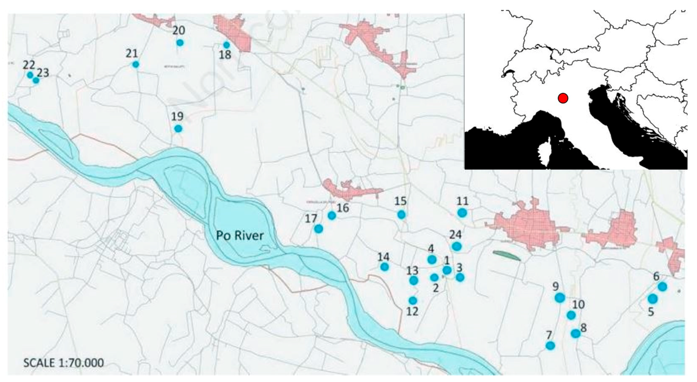
2.1. Data Collection

In this study we focused on the occurrence of the main zooplankton taxa in 24 pools and ponds that were randomly selected in a 200 km² area located in the Cremona province (central part of northern Italy) [50] (Figure 1).

Analyzed temporary pools and ponds, locally named bodri, have originated by flooding events of the Po River: erosive processes dug cone-shaped holes with depths up to 6–10 m and size varying between 1529 and 7070 m². Bodri generally display pronounced water level fluctuations, regulated by the Po river hydrometric level, precipitations, runoff, vertical migration of the aquifer, also due to irrigation, and summer evaporation. They represent spots of naturality within heavily exploited agricultural contexts and are vulnerable to diffuse pollution due to their small size. Many of the studied water bodies originated before 1723 [51] (for details see Table S1). At present, most bodri are eutrophic, undergo rapid infilling and display pronounced seasonal and daily variation of physico-chemical features. During surveys, they were characterised by the dominant form of primary producers (i.e., phytoplankton, submersed, floating leaves or emerged plants), for the level of saturation of dissolved gas of biological interest (i.e., O₂, CO₂, N₂ and CH₄), for dissolved nutrients (the inorganic forms of N, P and Si) and for sedimentary features (i.e., organic matter content).

Each pond was sampled twice: the first time between May and June 2014 and the second time between June and July 2015. Qualitative zooplankton samples were collected by 105 µm-mesh size plankton nets. Two to sixteen litres of water were filtered for each sample according to the estimated water volume and depth. All samples were preserved in 95% ethanol. All organisms present in the sample were sorted under a stereomicroscope and cladocerans were identified to genus level whereas copepods were distinguished in Calanoida and Cyclopoida. For each pond, 2 litres of water were sampled with a PE bottle. Nine chemical and three physical environmental descriptors were determined for each pond (Tables S2 and S3). Water temperature (wT), dissolved oxygen concentration, pH and electrical conductivity (EC) were measured in situ with a multiparameter probe (YSI model 566 MPS). In the laboratory, the water collected was filtered with Whatman GF/F filters (0.45 μm) and stored in glass vials (Labco Exetainer^®, Lampeter, Wales, UK) for the determination of dissolved inorganic carbon (DIC) [52] and soluble reactive phosphorus (SRP) [53], and in PE vials for the determination of dissolved reactive silica (SiO₂) [54], ammonium (NH₄⁺) [54] and nitrate (NO₃^–) [55] (Tables S2 and S3). Chlorophyll-a (Chla) concentration was determined spectrophotometrically after filtration of 100–500 mL of water (0.45 μm Whatman GF/F filters) and extraction of pigments with 90% acetone [54]. Besides physico-chemical and biological parameters, the ponds perimeter and main depth were also considered in the study as proxies of size [56] (Tables S2 and S3).

2.2. Environmental Features Selection

To avoid multicollinearity and to reduce redundant information from the set of environmental features, a score called variance inflation factor (VIF) was computed [57,58]. For a given predictor (p), the variance inflation factor measures how much the variance of a regression coefficient is inflated due to multicollinearity in the model. The smallest possible value of VIF is one (absence of multicollinearity). A VIF value that exceeds 5 or 10 indicates a problematic amount of collinearity [58]. In this work, as a conservative rule of thumb, a threshold equal to 4 was set. VIF was computed for all the environmental features with a stepwise procedure. The environmental features with VIF values > 4 were then excluded and the procedure was repeated until no environmental features with VIF greater than threshold remained.

2.3. Fuzzy Clustering

Fuzzy clustering aims at defining a membership value of an object that can be split between different clusters. The most common clustering method, the fuzzy c-means [59], bases the clustering procedure on the minimization of an objective function as reported in Equation (1):

$$\mathrm{J}(\mathrm{c})={\sum }_{\mathrm{i}=1}^{\mathrm{p}}{\sum }_{\mathrm{j}=1}^{\mathrm{c}}{\left({\mathsf{\mu }}_{\mathrm{i}\mathrm{j} }\right)}^{\mathrm{m}}{\mathrm{d}}_{\mathrm{i}\mathrm{j}}{}^2$$

(1)

where d_ij is the distance between the ith observation and jth centroid, p is the number of observations, c is the number of clusters (2 ≤ c ≤ n), μ_ij is the membership degree of the ith observation to the jth cluster and satisfying the following conditions:

μ_ij ∈ [0,1] for 1 ≤ i ≤ p, 1 ≤ j ≤ c
Σ μ_ij = 1 for 1 ≤ i ≤ p
Σ μ_ij > 0 for 1 ≤ j ≤ c

The exponent fuzzifier m defines the degree of fuzziness of the partition, when m approximates the value of 1, it operates as the k-means algorithm. Meanwhile, when m increases in value, the degree of fuzziness increases, and the fuzzy c-means leads to a solution where the memberships of each observation approximate 1/c [59]. The evaluation of the quality of the cluster procedure is made with a particular function that will be maximized or minimized according to the number of clusters c [60]. These procedures allow one to know how well the algorithm fitted the data structure (cluster validity problem). The most common measures for this task are the partition coefficient (PC) and the partition entropy (PE). In this study, the fuzzy c-means on the environmental dataset was used. The environmental features were standardized and a search grid procedure was used: the fuzzy c-means was run multiple times. For each run, a combination of the parameter c (number of cluster) and the fuzzifier exponent m, were set. The best partition was selected according to the maximum value of PC, or, in alternative, to the minimum value of PE. To improve the clustering procedure for each run, the algorithm was randomly initialized 50 times. The Principal Component Analysis (PCA) was performed as an operation of dimensionality reduction, in order to improve the visualization of the ponds with the membership values estimated from fuzzy c-means. The prototypes or the centroids of the estimated clusters, that are the values of the environmental features that characterized each cluster, were compared and the Trophic State Index (TSI) based on the values of prototype of the Chla was computed according to Carlson [61] using the Equation (2):

$$\mathrm{TSI}=10 (6-\frac{2.04-0.68\ln \mathrm{Chla}}{\ln 2})$$

(2)

To quantify the habitat heterogeneity of the environmental features, the Euclidean distances matrix between each observation (pond) and the median of each cluster were standardized and computed. Habitat heterogeneity was estimated by the average distance from the clusters’ medians [62]. The Permutational analysis of multivariate dispersions (PERMDISP) test for the analysis of multivariate homogeneity of groups was used [63]. PERMDISP compares within-group variance among clusters using the mean distance from individual observations to their cluster median. Bosco Bodini pond was excluded as it was dry in 2015 whereas two chemical parameters (NH4⁺ and DIC) were excluded due to multicollinearity in 2014. Square root corrections were applied for groups of unequal size [64] and to test differences in habitat heterogeneity among clusters, a permutation procedure (n = 999) was used. Average Euclidean distances from clusters’ medians were visualized in a reduced space with Principal Coordinate Analysis (PCoA). The analysis was carried out with the R package vegan [65].

2.4. Richness and Beta Diversity

For each year and for each cluster the taxa richness and the community structure were computed. The richness of the number of taxa observed was compared between clusters of the same year and by the Mann–Whitney U Test. Differences in Richness were tested also between years with the Wilcoxon Signed-Rank Test for paired samples. The alpha diversity (α) or the mean number of taxa were computed between years. The Sorensen index (βSOR) for presence/absence data was used as a measure of beta diversity for multiple sites [66]. The beta diversity was partitioned into two components: nestedness (βSNE) and turnover (βSIM). The overall beta diversity (βSOR) and its components were computed considering different years and different clusters within years. In order to compare βSOR between and within years, a resampling procedure was applied. An equal number of sites sampled (n = 5) and a total number of samples (n = 500) were set. This procedure allowed us to estimate the distributions of βSOR and the relative components, nestedness and turnover, for multiple sites with an equal number of ponds. The estimated distributions were compared with the Kolgomorov–Smirnov test. In order to highlight differences in zooplankton community diversity across time, pairwise measures of βSOR of each pond in two different years (2014 and 2015) were compared [67]. The βSOR analysis was carried out with the R package betapart [68].

2.5. Community Structure and Association Rules

Community structure was described by characteristic taxa and association rules mined from frequent pattern tree growth (FP-growth) and visualized by the frequent pattern tree (FP-tree). For each cluster, the characteristics of taxa were computed using the indices of presence (Pi) [13,69]. For each taxa, Pi was expressed as Pi = Pic/Nstc, where Pic is the i taxon belonging to a particular cluster, and Nstc is the number of ponds in a particular cluster. A taxon was identified as characteristic if its indices of presence were higher than the threshold Pi, set at 0.6 [13,69].

Considering the whole dataset of presence/absence data, association rules were extracted using frequent pattern growth algorithm (FP-growth), in order to highlight and evaluate correlations among co-occurrences of different taxa. An association rule is an implication X→Y that describes the existence of a relationship between X and Y species or group of species [22,70]. FP-growth is based on a divide-and-conquer approach, the algorithm identifies small patterns by decomposing the mining problem into a set of smaller ones represented by conditional databases, extracted on a compressed data representation, the FP-tree. This approach reduces the search space and the computational effort [23].

To select an association rule from the set of all possible rules, constraints of various quantitative measures of interestingness and significance were applied, using objective measures [71,72]. Interestingness measures the strength of the relationship between X and Y. As the first step of association rule mining, the threshold values of a support—confidence framework were used [73]. Support measures the probability of observing a particular group of species X in the dataset, while the confidence is the conditional probability of observing the species Y given the presence of the species X. A threshold value of minimum support equal to 0.1 and minimum confidence equal to 0.80 were set. The second step relied on an interestingness measure called lift. Lift quantifies the statistical dependence of two or more taxa in a particular rule; it is a positive real number, with a value equal to 1 under statistical independence [24]. Association rules were sorted in descending order of lift and association rules with lift value lower or equal to 1 were not considered [74]. The zooplankton community structure of each cluster was visualized in a compact way using the frequent pattern tree (FP-tree) [23,25]. Association rules were mined by Weka software version 3.8.4 [75] and visualized with the R packages Arules and ArulesViz [76,77].

3. Results

3.1. Environmental Features Selection

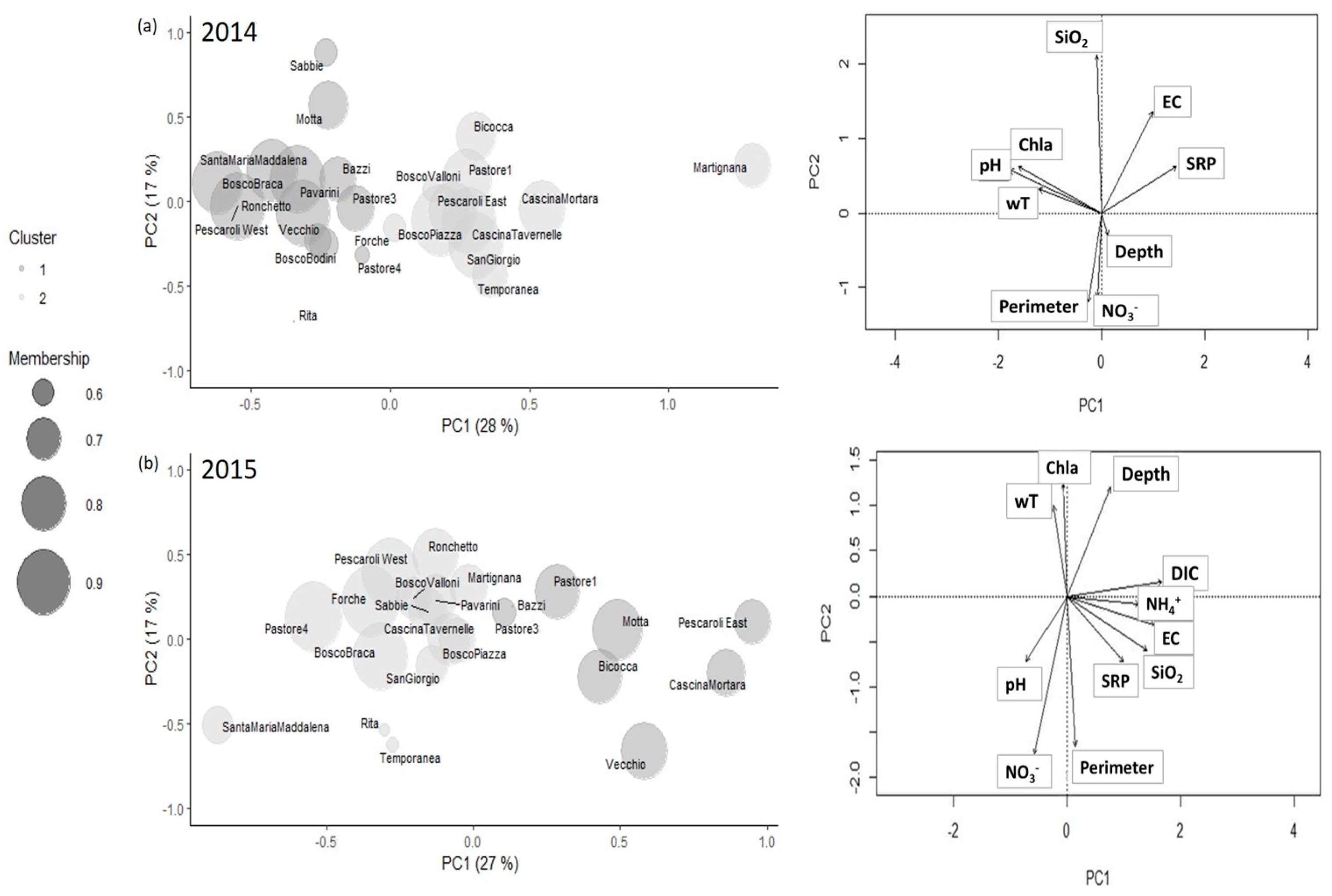
The analyzed shallow ponds exhibited pronounced variations of physico-chemical and biological parameters, reflecting different, site-specific equilibria between assimilative (e.g., oxygen-producing algal blooms, controlling nutrients) and dissimilative processes (e.g., heterotrophic microbial oxygen consumption recycling nutrients). During 2014 and 2015, most environmental features such as water temperature (wT), pH, conductivity (EC), soluble reactive phosphorus (SRP), nitrate (NO₃^–), chlorophyll-a (Chla), dissolved reactive silica (SiO₂), depth and perimeter showed values of VIF < 4 (

Table 1. VIF values for each chemical and physical environmental feature in 2014 and 2015.

Enviromental Features	VIF (2014)	VIF (2015)
Water temperature (wT)	1.40	1.69
pH	3.90	2.15
Oxygen (O2)	>4	>4
Conductivity (EC)	1.96	2.78
Ammonia (NH4+)	>4	3.88
Dissolved inorganic carbon (DIC)	>4	1.81
Soluble reactive phosphorus (SRP)	1.99	1.90
Nitrate (NO3−)	1.22	2.25
Chlorophyll-a (Chla)	2.38	1.29
Silica (SiO2)	2.06	2.60
Depth	1.33	1.97
Perimeter	1.32	1.74

). The selected variables were 9 in 2014 and 11 in 2015 according to VIF value > 4. Dissolved inorganic carbon (DIC) and ammonium (NH₄⁺) showed multicollinearity in 2014, whereas dissolved oxygen (O₂) showed multicollinearity in both years, and was removed from further analyses. Dissolved inorganic carbon (DIC) was positively correlated with conductivity (EC), ammonia (NH₄⁺), soluble active phosphorus (SRP) and reactive silica (SiO₂). Ammonium (NH₄⁺) was positively correlated with soluble reactive phosphorus (SRP) and negatively correlated with chlorophyll-a (Chla), pH and oxygen (O₂). In 2014, dissolved oxygen (O₂) was positively correlated with water temperature (wT), pH, chlorophyll-a (Chla), and negatively correlated with dissolved inorganic carbon (DIC), soluble reactive phosphorus (SRP) and ammonium (NH₄⁺) (Figure S1). In 2015, oxygen (O₂) was positively correlated with pH and nitrate (NO₃^–), whereas ammonium (NH₄⁺) and dissolved inorganic carbon (DIC) showed values of VIF < 4.

3.2. Fuzzy c-Means

In both years, the number of clusters was c = 2, corresponding to a value of the fuzzifier m = 1.5 (Figure S2). The evaluation of the quality of the clustering was made considering the best partition of the maximum value of partition coefficient (PC) and the minimum value of partition entropy (PE). In 2014 and 2015, the maximum value of PC, 0.68 and 0.63, respectively, and the minimum value of PE, 0.49 and 0.56, respectively, were obtained for c = 2. In 2014, the highest membership associated with Cluster 1 was observed for Pavarini, Pescaroli West and Santa Maria Maddalena, and with Cluster 2 for Bosco Piazza, San Giorgio and Cascina Tavernelle (

Table 2. Freshwater pond’s membership for each cluster in the year 2014 and 2015.

Ponds	2014		2015
	Cluster 1	Cluster 2	Cluster 1	Cluster 2
Pastore 3	0.72	0.28	0.63	0.37
Pastore 1	0.14	0.86	0.77	0.23
Pastore 4	0.56	0.432	0.11	0.89
Temporanea	0.30	0.70	0.41	0.59
Bosco Braca	0.88	0.12	0.13	0.87
Pavarini	0.93	0.07	0.26	0.74
Bosco Valloni	0.41	0.59	0.31	0.69
San Giorgio	0.08	0.92	0.33	0.67
Forche	0.39	0.61	0.10	0.90
Martignana	0.29	0.71	0.29	0.71
Santa Maria Maddalena	0.88	0.12	0.34	0.66
Bosco Bodini	0.65	0.35	-	-
Cacina Mortara	0.18	0.82	0.72	0.28
Bosco Piazza	0.03	0.97	0.30	0.70
Cascina Tavernelle	0.09	0.91	0.25	0.75
Vecchio	0.63	0.37	0.79	0.21
Bazzi	0.72	0.28	0.57	0.43
Motta	0.75	0.25	0.81	0.19
Ronchetto	0.91	0.09	0.22	0.77
Rita	0.54	0.46	0.42	0.58
Bicocca	0.26	0.74	0.77	0.23
Pescaroli West	0.93	0.072	0.12	0.88
Pescaroli East	0.17	0.83	0.70	0.30
Sabbie	0.61	0.39	0.28	0.72

). In 2015, the highest memberships associated to Cluster 1 and 2 were observed for Motta, Bicocca and Pastore 1, and for Pastore 4, Bosco Braca and Pescaroli West, respectively. In 2014, the prototypes showed that ponds in Cluster 1 were characterized by higher values of wT, pH, Chla, SiO₂, depth and perimeter and lower values of EC, SRP andNO₃^– than ponds in Cluster 2 (Figure 2 and Figure 3). In 2015, the ponds grouped in Cluster 1 were characterized by lower values of pH, Chla and higher values of EC, NH₄⁺, DIC, SRP, NO₃^–, reactive silica (SiO₂), depth and perimeter than ponds in Cluster 2. The wT of Cluster 1 was similar to that of Cluster 2 (

Table 3. Cluster’s prototypes of each environmental feature in the 2014 and 2015.

Enviromental Features	Prototypes 2014		Prototypes 2015
	Cluster 1	Cluster 2	Cluster 1	Cluster 2
Water temperature (wT)	20.29	17.69	23.49	23.92
pH	8.00	7.63	7.67	7.71
Conductivity (EC)	542.18	673.30	584.32	364.03
Ammonia (NH4+)	-	-	3.58	2.35
Dissolved inorganic carbon (DIC)	-	-	0.65	0.24
Soluble reactive phosphorus (SRP)	0.058	0.18	0.098	0.044
Nitrate (NO3–)	0.11	0.17	0.17	0.15
Chlorophyll-a (Chla)	2.70	0.90	3.44	4.46
Silica (SiO2)	2.44	2.24	14.30	7.47
Depth	4.28	4.18	4.50	4.02
Perimeter	209.08	205.97	221.58	204.73

). In 2015, both clusters estimated by fuzzy c-means showed higher values of the prototypes relative to wT, Chla and SiO₂, compared to the prototypes of clusters estimated in 2014. In 2014, the difference of trophic status between clusters was higher than in 2015. In 2014, the TSI was 40.30 for Cluster 1 and 29.56 for Cluster 2, while in 2015, it was 42.70 for Cluster 1 and 45.23 for Cluster 2. Ponds that, in both years, remained grouped in the same cluster were Pastore 3, Vecchio, Bazzi and Motta, grouped in Cluster 1, and Temporanea, Bosco Valloni, San Giorgio, Forche, Martignana, Bosco Piazza and Cascina Tavernelle, grouped in Cluster 2. Habitat heterogeneity, estimated by the average distance from clusters’ median, was 2.10 (Cluster 1) and 2.30 (Cluster 2) in 2014, while it raised to 3.10 (Cluster 1) and 2.54 (Cluster 2) in 2015 (Figure S3). The permutation test showed that habitat heterogeneity was not significantly different among clusters (F3 = 1.3103, p-value = 0.273).

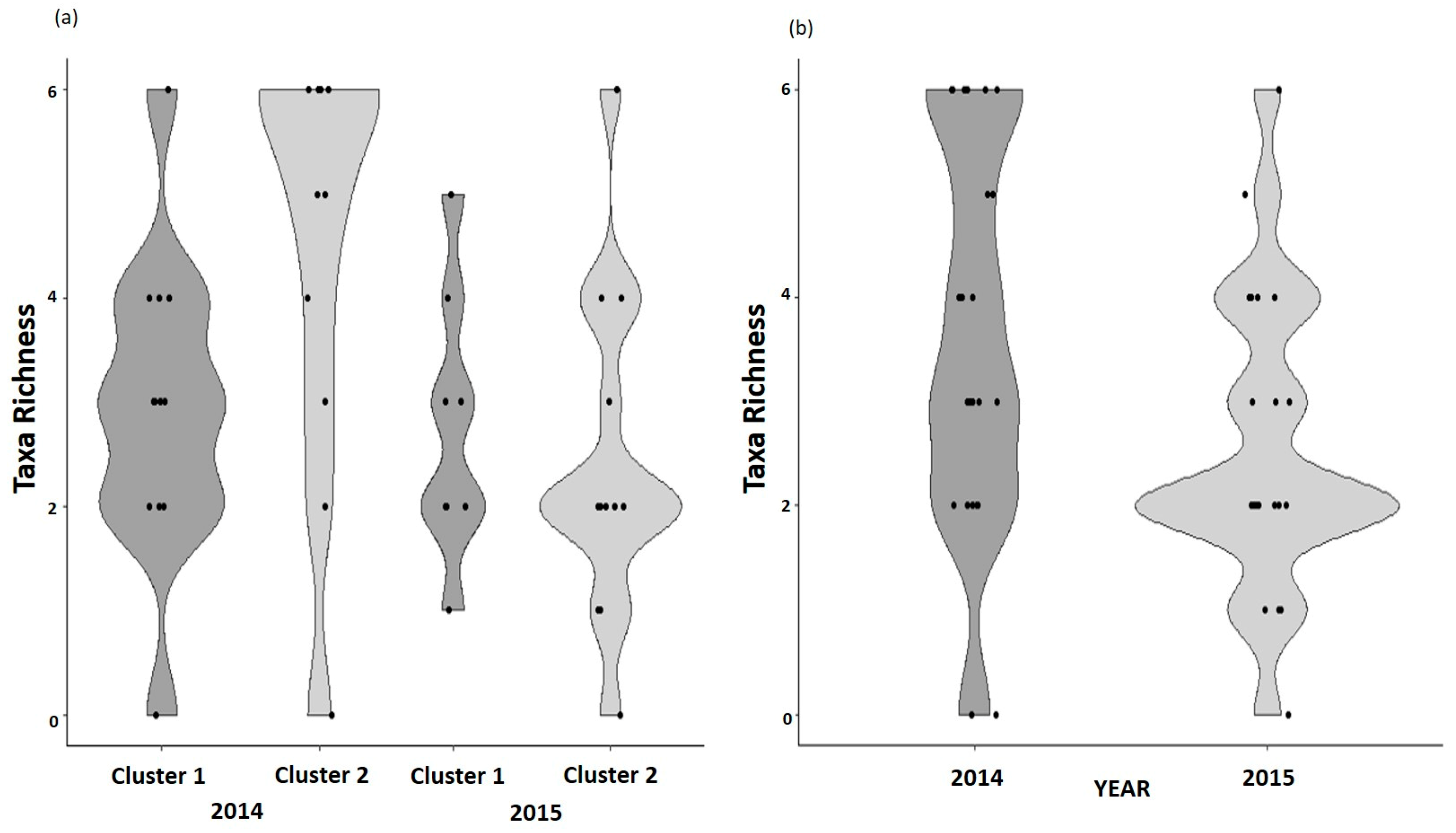
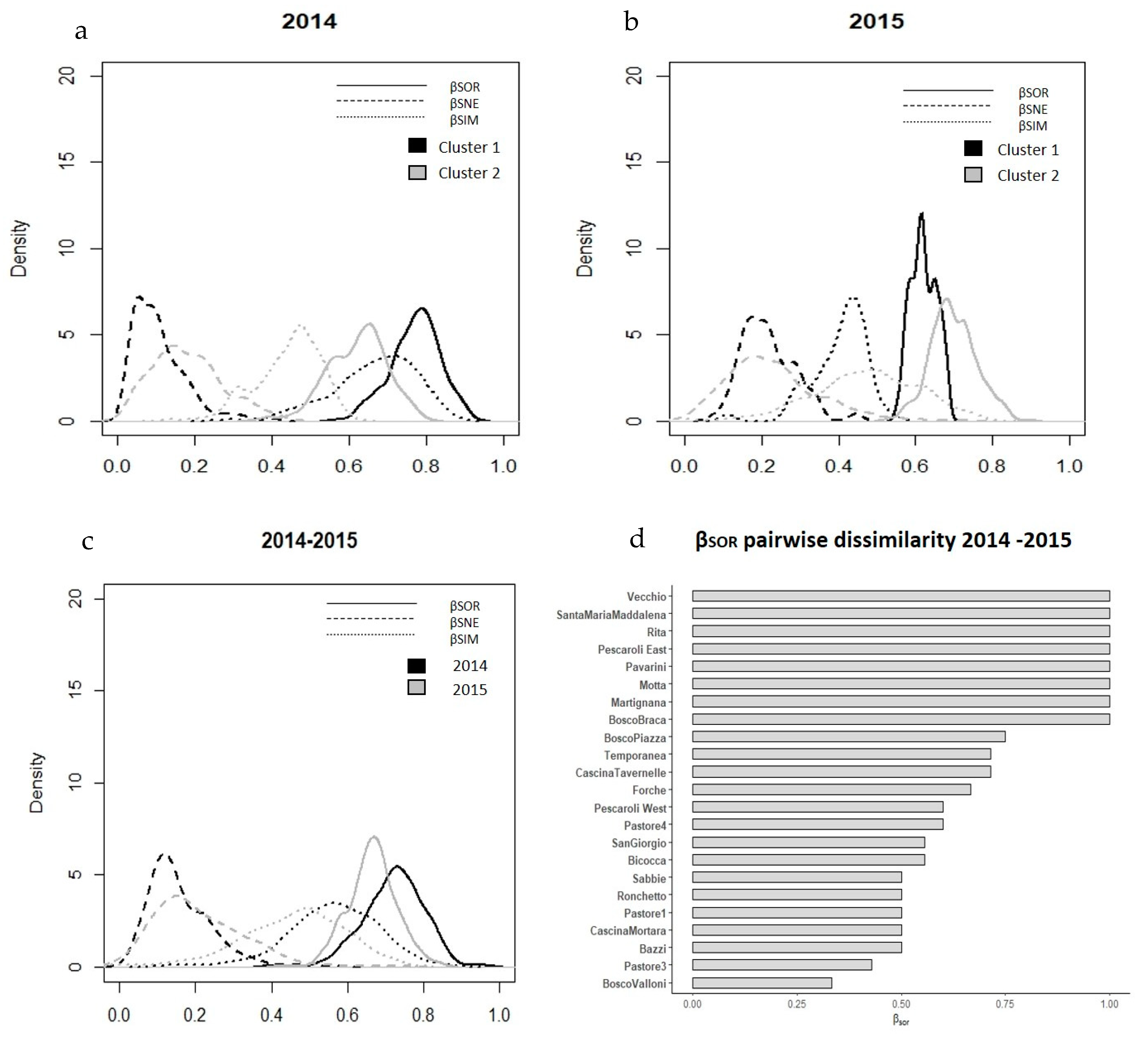
3.3. Richness and Beta Diversity

In 2014, the taxa richness was significantly lower in Cluster 1 than in Cluster 2 (W = 35.5 and p-value = 0.036), whereas in 2015 there was no significant difference between clusters (W = 69 and p-value = 0.5651) (Figure 3). Richness was higher in 2014 than in 2015 (V = 152.5, p-value = 0.02) (Figure 3), with values of alpha diversity (α) equal to 3.61 in 2014 and to 2.56 in 2015. The distributions of beta diversity index (βSOR) and the relative components nestedness (βSNE) and turnover (βSIM), estimated by resampling, were statistically different considering clusters and years (Table S4 and Figure 4). In 2014, the overall beta diversity (βSOR) and the turnover (βSIM) were higher than in 2015, but the nestedness (βSNE) was lower in 2014 than in 2015 (

Table 4. Beta diversity and the relative components nestedness (βSNE) and turnover (βSIM), computed for different cluster and year; α was the p-value of the results obtained with the Kolmogorov–Smirnov test after the permutation procedure.

Beta Diversity	2014			2015			Overall 2014	Overall 2015	α
	Cluster 1	Cluster 2	α	Cluster 1	Cluster 2	α
βSOR	0.85	0.76	<0.0001	0.71	0.84	<0.0001	0.89	0.87	<0.0001
βSNE	0.07	0.14	<0.0001	0.19	0.15	<0.0001	0.07	0.12	<0.0001
βSIM	0.78	0.61	<0.0001	0.52	0.69	<0.0001	0.82	0.75	<0.0001

and Figure 4).

In 2014, beta diversity (βSOR) and turnover (βSIM) were higher in Cluster 1 than in Cluster 2, but nestedness (βSNE) was lower in Cluster 1 than in Cluster 2. In 2015, beta diversity (βSOR) and turnover (βSIM) were higher in Cluster 2 than in Cluster 1, but the nestedness (βSNE) component was higher in Cluster 1 than in Cluster 2 (Table 4 and Figure 4). The pairwise comparison of beta diversity (βSOR) between ponds in different years was the maximum (βSOR = 1) for Vecchio, Santa Maria Maddalena, Rita, Pescaroli East, Pavarini, Motta, Martignana and Bosco Braca, while the minimum value was recorded for Bosco Valloni (βSOR = 0.33) (Figure 4).

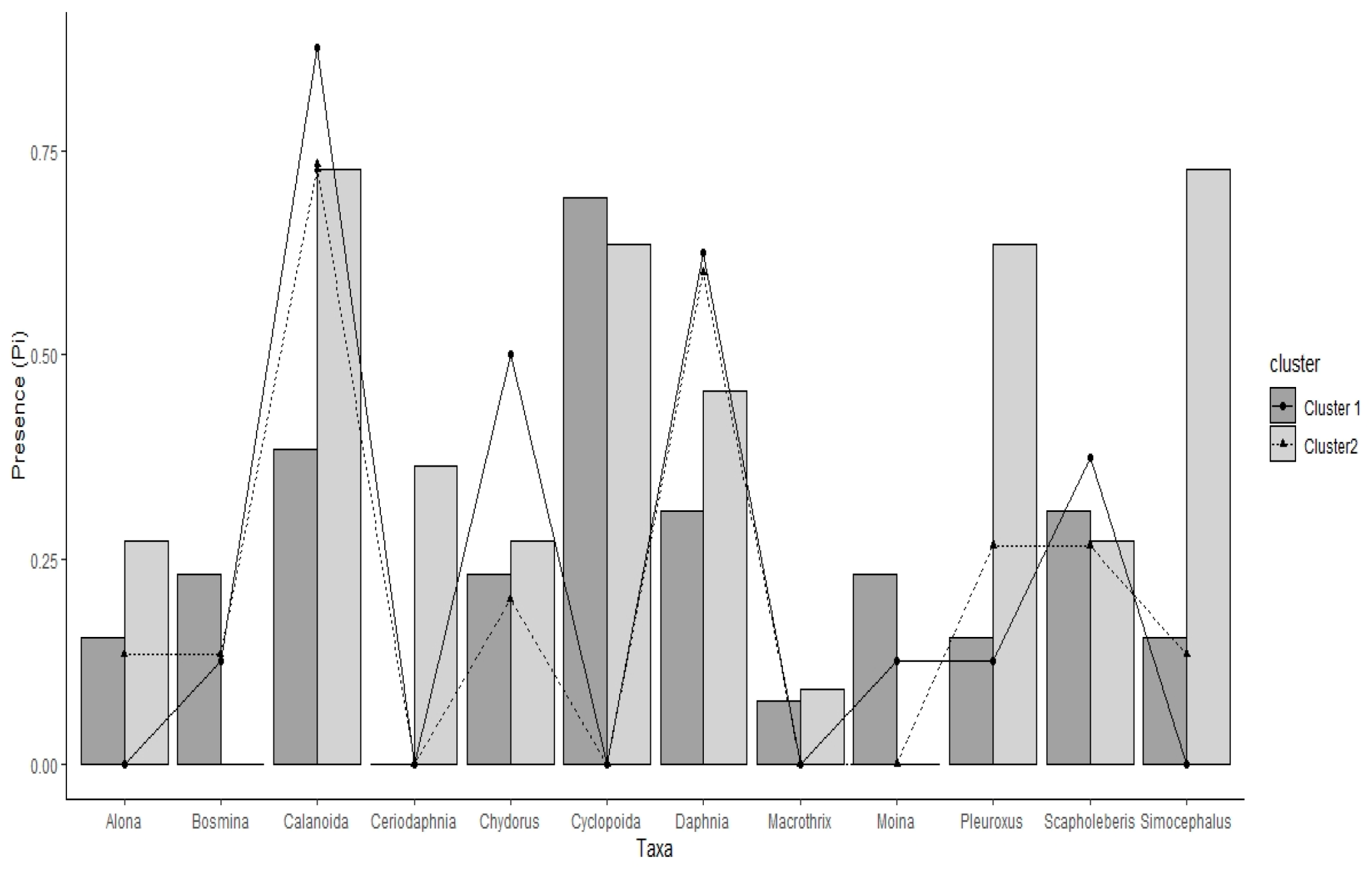
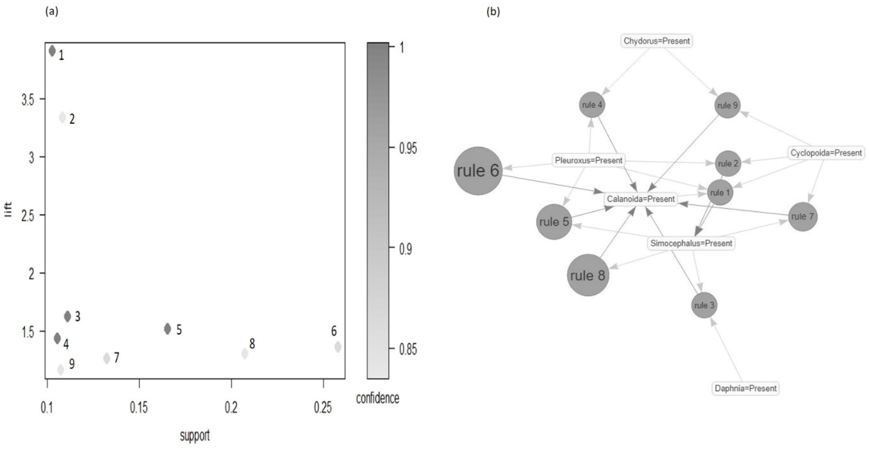
3.4. Community Structure and Association Rules

In 2014, the characteristic taxa were Calanoida (Pi = 0.69) for Cluster 1 and Simochephalus (0.72), Calanoida (0.72), Pleuroxus (0.64), and Cyclopoida (0.63) for Cluster 2. In 2015, the characteristic taxa of both clusters were represented by Calanoida (Cluster 1 = 0.87 and Cluster 2 = 0.73) and Daphnia (Cluster 1 = 0.62 and Cluster 2 = 0.63) (Figure 5). Considering the whole dataset, nine association rules were found (Figure 6 and Table S5). One association rule showed higher values of lift (3.92) and indicated the co-occurrence of Calanoida, Cyclopoida and Pleuroxus with Simocephalus. This association was found in ponds of Cluster 2 in 2014. Three association rules with lift values equal to 1.52 indicated the co-occurrence of Daphnia, Simocephalus, Chydorus and Pleuroxus with Calanoida (Table S5).

These associations were found in Cluster 2 of both years 2014 and 2015 and in Cluster 1 of 2015. The association rule with the lowest lift value (lift = 1.26) indicated the co-occurrence of Chydorus and Cyclopoida with Calanoida and was found in both Clusters 1 and 2, in 2014. The f requent pattern tree (FPt) revealed different patterns in the community structure between clusters and years. In 2014, most of the ponds of Cluster 1 were characterized by the presence of Calanoida and Cyclopoida, whereas the community structure of Cluster 2 was characterized by the co-occurrence of Simocephalus, Calanoida, Pleuroxus and Cyclopoida (Figure 7 and Figure S4) as expressed by the first association rule with the highest value of lift. In 2015, the community structure of Cluster 1 was characterized by the presence of Calanoida, Daphnia and Chydorus while Cluster 2 was characterized by the presence of Calanoida, Daphnia and Scapholeberis (Figure 7 and Figure S4).

4. Discussion

Results from this study suggest that shallow ponds may undergo completely different trajectories in the same geographical area and may display pronounced differences in terms of their water’s physico-chemical and biological parameters. This is not surprising due to their overall small size and to the small ratio between their water volume and sediment surface. The small water volume has limited buffer capacity against climatic anomalies, water ingression from the aquifer or from the watershed, resulting in local, sharp changes of physico-chemical parameters and, as a consequence, of biological communities [78,79,80].

Phytoplankton communities have, in turn, the potential to control inorganic nutrients and regulate dissolved oxygen, inorganic carbon concentrations and water pH. Assimilative processes are contrasted by nutrient regeneration from sediments that, together with the low ratio between water volume and sediment surface, amplify the effects produced by microbial dissimulative pathways (e.g., oxygen shortage) [79]. However, the most interesting result of this study does not deal with different solutes or chlorophyll concentrations in the analyzed shallow water ecosystems. Ponds are intrinsically heterogeneous, they can be net autotrophic or net heterotrophic and these extremes correlate with high chlorophyll, oxygen and low nutrient concentrations or the opposite, respectively [78]. What is novel here is that the functioning of ponds, exemplified by snapshots showing phytoplankton, nutrient concentrations and zooplankton community composition, may diverge from year to year due to some sort of continuous disturbance or to the absence of a stable steady state. Such instability is favored by the vulnerability of ponds to a large set of pressures and may contribute to the paradox of their diversity, which is a central topic in recent freshwater research and has important implications for ecosystem restoration, in particular in heavily impacted agricultural areas [78,79].

The main findings of this study were extracted from the dataset via the application of an unsupervised machine learning and data mining algorithm, fuzzy c-means and frequent pattern growth. Such an approach allowed us to assess the factors that influenced assemblage composition and the apparently erratic distribution patterns of zooplankton taxa in 24 ponds and in two consecutive years. Data in ecology are characterized by high uncertainty, bias and a hierarchical level of complexity. Machine learning tools were used according to the level of complexity of ecological systems in order to understand environmental and biological dynamics [81], shift in species assemblages along time [12] and to plan conservation actions for ecological communities threatened by anthropic pressure and climate change [82]. Classical clustering methods generally define sharp boundaries between groups and each object belongs only to a particular cluster. These classical procedures do not consider the continuous realm of ecological features. The assumptions based on Boolean rules might lead to misclassifications and might fail to detect outliers. A set of ecological objects, in our case the freshwater ponds, can be partitioned using fuzzy logic, where a probabilistic approach helps to capture the continuous nature of ecological data.

Brownscombe et al. [3] applied supervised machine learning techniques combined with unsupervised fuzzy c-means to a wide range of informational sources in order to identify potential spawning aggregation sites for a marine fish species. The flexibility and the probabilistic output of the fuzzy logic, with respect to the classical partition procedure based on crispy clustering, was used to describe species association in marine ecosystems that consist of communities or cohesive units of not-random taxa groups and assemblages of taxa that are randomly associated [13]. Fuzzy clustering algorithms were used also for the identification and partition of similar regions and hydrologically homogeneous watersheds [83].

In this study, for both years, the fuzzy c-means algorithm allowed us to identify two different clusters. In 2014, ponds in Cluster 1 were characterized by high concentrations of chlorophyll-a, high pH and water temperature while ponds in Cluster 2 were characterized by high concentrations of chemical species, with silica as the only exception. Cluster 1 was more autotrophic and showed a higher TSI than Cluster 2. In 2015, temperature was comparable between clusters and the situation of 2014 was reversed, with Cluster 1 more heterotrophic and characterized by a higher concentration of chemical species (SRP, DIC, NH₄⁺, NO₃⁻), higher conductivity, depth and perimeter and lower values of pH than Cluster 2. In different years, the chemistry of water changed in many ponds, and large differences were recorded in Pastore 3, Vecchio, Bazzi and Motta, where the concentrations of all chemical parameters increased and a reduction of pH was recorded. In contrast, Temporanea, Bosco Valloni, San Giorgio, Forche, Martignana, Bosco Piazza and Cascina Tavernelle showed a reduction in the concentration of nutrients and of electrical conductivity. In 2015, all ponds showed higher concentrations of chlorophyll-a than in 2014, confirmed by the increase of the trophic state index. This result was probably due to the effect of higher temperatures in 2015 than in 2014. Differences between cluster communities might be related to different factors, among which the amount and the quality of water inputs from runoff, from the aquifer or the thermal regime in winter and late spring. A general increase in the concentration of reactive silica was observed in 2015 as compared to 2014, likely due to regeneration from sediments uncoupled to uptake. Fuzzy c- means identified a pond (Rita) with the lowest value of cluster membership in both years and the highest value of nitrate, likely due to diffuse inputs. The zooplankton community structure (species richness and species composition) is potentially affected by both water chemistry and site morphology, and by anthropogenic pressures in lakes and watersheds [33,84,85]. At the geographical level, the species pool is driven by dispersal constraint, whereas the habitat species pool is due to environmental constrains [86]. The high taxonomic diversity in zooplankton communities is only partially expressed in individual freshwater habitats and the differences in zooplankton community structures among systems is largely associated with specific environmental conditions [87,88,89]. Abiotic factors (e.g., pH, temperature, light intensity) can also influence the zooplankton community structure of fishless aquatic habitats directly by sorting species based on differential physiological tolerances, or indirectly by interacting with biotic conditions such as primary production and invertebrate predation [90,91,92]. The observed taxa are also determined by internal dynamics due to biotic factors, such as predation, intraspecific and interspecific competition. A particular pattern of taxa was the result of internal and external process that defined the community structure.

In this work, a data mining algorithm was used to evaluate the co-occurrence of taxa on presence–absence data in a system of freshwater ponds. This method allowed us to quantify possible correlations among taxa in frequent patterns extracted from data and to highlight differences in the community structure between consecutive years. In 2014, the taxa richness was higher in Cluster 2 than in Cluster 1 and the community structure was different. Cluster 2 was dominated by the presence of Simocephalus in many ponds, while in Cluster 1 the taxa with a higher presence were Cyclopoida and Calanoida. Furthermore, Simocephalus was not present in ponds characterized by higher pH in both years. In 2014, Pastore 4 showed the lowest value of membership for Cluster 1: all environmental features were similar to prototypes of Cluster 1 except for chloropyll-a and reactive silica, that were more similar to Cluster 2. However, the community structure in Pastore 4 was composed of Cyclopoida, Calanoida and Daphnia, which was the most frequent pattern in Cluster 1. In 2014, the community structure was characterized by not-common taxa association composed by Pleuroxus, Alona, Moina and Macrothrix, while, in 2015, the presence of these taxa was not recorded. The smallest membership associated to a particular cluster was found for ponds belonging to the group with the lowest nutrient concentrations. In both years, a low beta diversity was observed for clusters with higher concentrations of chemical species, high conductivity and pH.

In general, nestedness of species assemblages occurs when the biota of sites with smaller numbers of species are subsets of the biota at richer sites [93,94], reflecting a non-random process of species loss as a consequence of any factor that promotes the orderly disaggregation of assemblages [95]. Turnover implies the replacement of some species by others, as a consequence of environmental sorting or spatial and historical constraints [96]. The environmental features working as a driver at the local scale might have shaped the community assemblage, decreasing the species replacement between the ponds as shown by a lower turnover. As reported in Gianuca et al. [97] a higher heterogeneity usually produces turnover patterns but, in our study, from PERMDISP analysis, a difference in heterogeneity among clusters was not recorded. In this work, the ponds characterized by lower nutrient concentrations showed higher turnover. In clusters with a higher value of trophic status, the component of nestedness increased, that is poorest ponds in taxa richness were subsets of the richest ponds. A nestedness pattern may highlight an internal cluster gradient of environmental features that might drive the community assemblage. Margalef [98] gave rise to the widespread concept that the lower the level of lake eutrophication, the more complex the structure of aquatic animal communities. A general reduction in taxa richness was observed in 2015 compared to 2014, suggesting a tendency to a higher trophic status of both clusters. The higher temperatures of the water in 2015 may have favored the increase of phytoplankton production. In 2015, a general reduction in the complexity of the community structure was observed compared to 2014. This condition was highlighted by the FP-tree. In 2015, the community structure was characterized by Calanoida and Daphnia. Calanoid copepods generally appear to be best adapted to oligotrophic conditions, whilst cyclopoid copepods and cladocerans are relatively more abundant in eutrophic waters [99,100]. In our study, the presence of Cladocera decreased between years, but Cyclopoida disappeared with the highest trophic status observed in 2015. Variation in community structure alters ecosystem functioning and biodiversity metrics can indicate how communities influence ecosystems [101,102,103,104]. Seasonal and interannual increases in Daphnia abundance have been associated with P limitation due to higher requirements in Daphnia than in other taxa [105]. Moreover, filtrator Daphnia species fed on the smallest food particles with a low selectivity, while many species of cyclopoids show a raptorial feeding type and high selectivity preferences of much larger food items [106]. Chydorids are more successful in very productive habitats, feeding by scraping algal particles from periphyton. On the contrary, Bosmina shows the lowest clearance rate, declines with increasing food concentrations and does not co-occur with Daphnia [106]. However, information about food quality and quantity as well as adaptive life history strategy needs to understand the mechanistic role of association rules in ecosystem functioning. In perspective, information on taxa’s functional traits might be included in analysis by unsupervised machine learning.

Results from physico-chemical and biological (e.g., chlorophyll-a and zooplankton communities) analysis of shallow ponds reveals large variability of all single (e.g., nitrate, pH) and aggregated (e.g., trophic status, biodiversity indexes) parameters over short temporal scales. Under such conditions, traditional statistical approaches may fail to extract significant patterns or aggregations, and consider them as erratic. Fuzzy logic allowed us to group ponds in clusters that differed in two consecutive years, likely due to small differences in external stressors, affecting the unstable equilibrium between autotrophic and heterotrophic processes and their dominance. The latter, in turn, affect nutrient concentrations and the intensity of algal blooms, producing cascading consequences on zooplankton diversity and community composition. Year-to-year slight variations in water temperatures, different timing, absence of diffuse nutrient input via runoff and variable interactions with the aquifer may drive timing of blooms but also the intensity of heterotrophic microbial activities in sediments of shallow ponds. Such variations result in dynamic rearrangement of ponds in clusters, and might end up in excess nutrients sustaining algal growth or in nutrient limitation, stimulating zooplankton richness.

5. Conclusions

This study represents an example of a promising application of machine learning techniques applied to a heterogeneous dataset. The fuzzy-set theory provided a mathematical approach that was able to cope with imprecision and allowed us to cluster ponds without defining discrete boundaries. Such an approach allowed us to assess the factors that influenced assemblage composition and the apparently erratic distribution patterns of zooplankton taxa. In our case, the freshwater ponds were partitioned with a probabilistic approach that allowed us to capture the continuous nature of ecological data.

References

1. Rammer, W.; Seidl, R. Harnessing Deep Learning in Ecology: An Example Predicting Bark Beetle Outbreaks. Front. Plant Sci. 2019, 10, 1327. [Google Scholar] [CrossRef] [PubMed]
2. Christin, S.; Hervet, É.; le Comte, N. Applications for deep learning in ecology. Methods Ecol. Evol. 2019, 10, 1632–1644. [Google Scholar] [CrossRef]
3. Brownscombe, J.W.; Griffin, L.P.; Morley, D.; Acosta, A.; Hunt, J.; Lowerre-Barbieri, S.K.; Adams, A.J.; Danylchuk, A.J.; Cooke, S.J. Application of machine learning algorithms to identify cryptic reproductive habitats using diverse information sources. Oecologia 2020, 194, 1–16. [Google Scholar] [CrossRef] [PubMed]
4. Crisci, C.; Ghattas, B.; Perera, G. A review of supervised machine learning algorithms and their applications to ecological data. Ecol. Model. 2012, 240, 113–122. [Google Scholar] [CrossRef]
5. Lek, S.; Guégan, J. Artificial neural networks as a tool in ecological modelling, an introduction. Ecol. Model. 1999, 120, 65–73. [Google Scholar] [CrossRef]
6. Olden, J.D.; Lawler, J.J.; Poff, N.L. Machine Learning Methods Without Tears: A Primer for Ecologists. Q. Rev. Biol. 2008, 83, 171–193. [Google Scholar] [CrossRef] [Green Version]
7. Recknagel, F. Applications of machine learning to ecological modelling. Ecol. Model. 2001, 146, 303–310. [Google Scholar] [CrossRef]
8. Armitage, D.W.; Ober, H.K. A comparison of supervised learning techniques in the classification of bat echolocation calls. Ecol. Inform. 2010, 5, 465–473. [Google Scholar] [CrossRef]
9. Lumini, A.; Nanni, L. Deep learning and transfer learning features for plankton classification. Ecol. Inform. 2019, 51, 33–43. [Google Scholar] [CrossRef]
10. Mellios, N.; Moe, S.J.; Laspidou, C. Machine Learning Approaches for Predicting Health Risk of Cyanobacterial Blooms in Northern European Lakes. Water 2020, 12, 1191. [Google Scholar] [CrossRef] [Green Version]
11. Lee, K.Y.; Chung, N.; Hwang, S. Application of an artificial neural network (ANN) model for predicting mosquito abundances in urban areas. Ecol. Inform. 2016, 36, 172–180. [Google Scholar] [CrossRef] [Green Version]
12. Chon, T.-S.; Park, Y.-S.; Park, J.H. Determining temporal pattern of community dynamics by using unsupervised learning algorithms. Ecol. Model. 2000, 132, 151–166. [Google Scholar] [CrossRef]
13. Fiorentino, D.; Pesch, R.; Guenther, C.-P.; Gutow, L.; Holstein, J.; Dannheim, J.; Ebbe, B.; Bildstein, T.; Schroeder, W.; Schuchardt, B.; et al. A ‘fuzzy clustering’ approach to conceptual confusion: How to classify natural ecological associations. Mar. Ecol. Prog. Ser. 2017, 584, 17–30. [Google Scholar] [CrossRef] [Green Version]
14. Sperlea, T.; Kreuder, N.; Beisser, D.; Hattab, G.; Boenigk, J.; Heider, D. Quantification of the covariation of lake microbiomes and environmental variables using a machine learning-based framework. Mol. Ecol. 2021, 14. [Google Scholar] [CrossRef]
15. Suppa, A.; Kvist, J.; Li, X.; Dhandapani, V.; Almulla, H.; Tian, A.Y.; Kissane, S.; Zhou, J.; Perotti, A.; Mangelson, H.; et al. Roundup causes embryonic development failure and alters metabolic pathways and gut microbiota functionality in non-target species. Microbiome 2020, 8, 1–15. [Google Scholar] [CrossRef] [PubMed]
16. Zimmermann, H.J. Practical Applications of Fuzzy Technologies; Springer: Boston, MA, USA, 1999. [Google Scholar]
17. Salski, A. Fuzzy clustering of fuzzy ecological data. Ecol. Inform. 2007, 2, 262–269. [Google Scholar] [CrossRef]
18. Equihua, M. Fuzzy Clustering of Ecological Data. J. Ecol. 1990, 78, 519. [Google Scholar] [CrossRef]
19. Marsili-Libelli, S. Computer assisted vegetation analysis. In Handbook of Vegetation Science, 1st ed.; Feoli, E., Orloci, L., Eds.; Springer: Berlin/Heidelberg, Germany, 1991; Volume 11. [Google Scholar] [CrossRef]
20. Odeh, I.O.A.; McBratney, A.B.; Chittleborough, D.J. Soil Pattern Recognition with Fuzzy-c-means: Application to Classification and Soil-Landform Interrelationships. Soil Sci. Soc. Am. J. 1992, 56, 505–516. [Google Scholar] [CrossRef]
21. Friederichs, M.; Fränzle, O.; Salski, A. Fuzzy clustering of existing chemicals according to their ecotoxicological properties. Ecol. Model. 1996, 85, 27–40. [Google Scholar] [CrossRef]
22. Zhang, S.; Wu, X. Fundamentals of association rules in data mining and knowledge discovery. Wiley Interdiscip. Rev. Data Min. Knowl. Discov. 2011, 1, 97–116. [Google Scholar] [CrossRef]
23. Nasreen, S.; Azam, M.A.; Shehzad, K.; Naeem, U.; Ghazanfar, M.A. Frequent Pattern Mining Algorithms for Finding Associated Frequent Patterns for Data Streams: A Survey. Procedia Comput. Sci. 2014, 37, 109–116. [Google Scholar] [CrossRef] [Green Version]
24. Geng, L.; Hamilton, H.J. Interestingness measures for data mining. ACM Comput. Surv. 2006, 38, 24. [Google Scholar] [CrossRef]
25. Han, J.; Cheng, H.; Xin, D.; Yan, X. Frequent pattern mining: Current status and future directions. Data Min. Knowl. Discov. 2007, 15, 55–86. [Google Scholar] [CrossRef] [Green Version]
26. Céréghino, R.; Boix, D.; Cauchie, H.-M.; Martens, K.; Oertli, B. The ecological role of ponds in a changing world. Hydrobiologia 2014, 723, 1–6. [Google Scholar] [CrossRef] [Green Version]
27. De Meester, L.; Declerck, S.; Stoks, R.; Louette, G.; van de Meutter, F.; de Bie, T.; Michels, E.; Brendonck, L. Ponds and pools as model systems in conservation biology, ecology and evolutionary biology. Aquat. Conserv. Mar. Freshw. Ecosyst. 2005, 15, 715–725. [Google Scholar] [CrossRef]
28. Downing, A.L.; Leibold, M.A. Species richness facilitates ecosystem resilience in aquatic food webs. Freshw. Biol. 2010, 55, 2123–2137. [Google Scholar] [CrossRef]
29. Verdonschot, R.C.M.; Keizer-Vlek, H.E.; Verdonschot, P.F.M. Biodiversity value of agricultural drainage ditches: A comparative analysis of the aquatic invertebrate fauna of ditches and small lakes. Aquat. Conserv. Mar. Freshw. Ecosyst. 2011, 21, 715–727. [Google Scholar] [CrossRef]
30. Hassall, C. The ecology and biodiversity of urban ponds. Wiley Interdiscip. Rev. Water 2014, 1, 187–206. [Google Scholar] [CrossRef]
31. Céréghino, R.; Biggs, J.; Oertli, B.; Declerck, S. The ecology of European ponds: Defining the characteristics of a neglected freshwater habitat. Hydrobiologia 2008, 597, 1–6. [Google Scholar] [CrossRef]
32. Søndergaard, M.; Johansson, L.S.; Lauridsen, T.L.; Jørgensen, T.B.; Liboriussen, L.; Jeppesen, E. Submerged macrophytes as indicators of the ecological quality of lakes. Freshw. Biol. 2010, 55, 893–908. [Google Scholar] [CrossRef]
33. Dodson, S.; Arnott, S.; Cottingham, K. The relationhip in lake communities between primary productivity and species richness. Ecology 2000, 81, 2662–2679. [Google Scholar] [CrossRef]
34. Dzialowski, A.R. Invasive zebra mussels alter zooplankton responses to nutrient enrichment. Freshw. Sci. 2013, 32, 462–470. [Google Scholar] [CrossRef]
35. Kruk, C.; Rodríguez-Gallego, L.; Meerhoff, M.; Quintans, F.; Lacerot, G.; Mazzeo, N.; Scasso, F.; Paggi, J.C.; Peeters, E.T.H.M.; Marten, S. Determinants of biodiversity in subtropical shallow lakes (Atlantic coast, Uruguay). Freshw. Biol. 2009, 54, 2628–2641. [Google Scholar] [CrossRef]
36. Meerhoff, M.; Clemente, J.M.; de Mello, F.T.; Iglesias, C.; Pedersen, A.R.; Jeppesen, E. Can warm climate-related structure of littoral predator assemblies weaken the clear water state in shallow lakes? Glob. Chang. Biol. 2007, 13, 1888–1897. [Google Scholar] [CrossRef]
37. Pinto-Coelho, R.; Pinel-Alloul, B.; Méthot, G.; Havens, K.E. Crustacean zooplankton in lakes and reservoirs of temperate and tropical regions: Variation with trophic status. Can. J. Fish. Aquat. Sci. 2005, 62, 348–361. [Google Scholar] [CrossRef] [Green Version]
38. Wei, W.; Chen, R.; Wang, L.; Fu, L. Spatial distribution of crustacean zooplankton in a large river-connected lake related to trophic status and fish. J. Limnol. 2017, 76, 546–554. [Google Scholar] [CrossRef] [Green Version]
39. Belfiore, N.M. Effects of contaminants on genetic patterns in aquatic organisms: A review. Mutat. Res. Mutat. Res. 2001, 489, 97–122. [Google Scholar] [CrossRef]
40. Bossuyt, B.T.; Janssen, C.R. Copper toxicity to different field-collected cladoceran species: Intra- and inter-species sensitivity. Environ. Pollut. 2005, 136, 145–154. [Google Scholar] [CrossRef]
41. Guan, R.; Wang, W.-X. Multigenerational cadmium acclimation and biokinetics in Daphnia magna. Environ. Pollut. 2006, 141, 343–352. [Google Scholar] [CrossRef]
42. Hanazato, T. Influence of food density on the effects of a Chaoborus-released chemical on Daphnia ambigua. Freshw. Biol. 1991, 25, 477–483. [Google Scholar] [CrossRef]
43. Hunter, K.; Pyle, G. Morphological Responses of Daphnia Pulex to Chaoborus Americanus Kairomone in the Presence and Absence of Metals. Environ. Toxicol. Chem. 2004, 23, 1311–1316. [Google Scholar] [CrossRef]
44. Schindler, D.W. The cumulative effects of climate warming and other human stresses on Canadian freshwaters in the new millennium. Can. J. Fish. Aquat. Sci. 2001, 58, 18–29. [Google Scholar] [CrossRef]
45. Schindler, D.W. Lakes as sentinels and integrators for the effects of climate change on watersheds, airsheds, and landscapes. Limnol. Oceanogr. 2009, 54, 2349–2358. [Google Scholar] [CrossRef]
46. Riessen, H.P. Costs of predator-induced morphological defences in Daphnia. Freshw. Biol. 2012, 57, 1422–1433. [Google Scholar] [CrossRef]
47. Vadadi-Fülöp, C.; Sipkay, C.; Mészáros, G.; Hufnagel, L. Climate change and freshwater zooplankton: What does it boil down to? Aquat. Ecol. 2012, 46, 501–519. [Google Scholar] [CrossRef] [Green Version]
48. Rotiroti, M.; Bonomi, T.; Sacchi, E.; McArthur, J.M.; Stefania, G.A.; Zanotti, C.; Taviani, S.; Patelli, M.; Nava, V.; Soler, V.; et al. The effects of irrigation on groundwater quality and quantity in a human-modified hydro-system: The Oglio River basin, Po Plain, northern Italy. Sci. Total. Environ. 2019, 672, 342–356. [Google Scholar] [CrossRef] [PubMed]
49. Rossi, V.; Maurone, C.; Benassi, G.; Marková, S.; Kotlík, P.; Bellin, N.; Ferrari, I. Phenology of Daphnia in a Northern Italy pond during the weather anomalous 2014. J. Limnol. 2015, 74, 74. [Google Scholar] [CrossRef] [Green Version]
50. Marková, S.; Maurone, C.; Racchetti, E.; Bartoli, M.; Rossi, V. Daphnia diversity in water bodies of the Po River Basin. J. Limnol. 2016, 76, 261–271. [Google Scholar] [CrossRef] [Green Version]
51. AAVV. Appunti Sulla Golena del Po. Le Lanche di Motta e Torricella del Pizzo; Comune di Cremona: Cremona, Italy, 1999. [Google Scholar]
52. Anderson, L.G.; Hall, P.O.J.; Iverfeldt, A.; van der Loejf, M.M.R.; Sundby, B.; Westerlund, S.F.G. Benthic respiration measured by total carbonate production. Limnol. Oceanogr. 1986, 31, 319–329. [Google Scholar] [CrossRef] [Green Version]
53. Valderrama, J.C. Methods Used by the Hydrographical Department of the National Board of Fisheries. In Report of the Baltic Intercalibration Workshop. Annex; Grasshof, K., Ed.; Interim Commission for the Protection of the Environment of the Baltic Sea: Goteborg, Sweden, 1977; pp. 14–43. [Google Scholar]
54. Water Environmental Federation; American Public Health Association. Standard Methods for the Examination of Water and Wastewater; APHA: Washington, DC, USA, 1981. [Google Scholar]
55. Rodier, J.; Legube, B.; Merlet, N. L’Analyse de l’ Eau; Dunod: Paris, France, 1987. [Google Scholar]
56. D’Auria, G.; Zavagno, F. Indagine sui Bodri della Provincia di Cremona. Monogr. Pianura 1999, 3, 5–229. [Google Scholar]
57. Bruce, P.; Bruce, A. Practical Statistics for Data Scientists; O’Reilly Media: Sebastobol, CA, USA, 2017. [Google Scholar]
58. James, G.; Daniela, W.; Trevor, H.; Robert, T. An Introduction to Statistical Learning: With Applications in R; Springer Publishing Company, Inc: New York, NY, USA, 2014. [Google Scholar]
59. Tilson, L.; Excell, P.; Green, R. A Generalisation of The Fuzzy C-means Clustering Algorithm. Int. Geosci. Remote Sens. Symp. Remote Sens. 2005, 3, 1783–1784. [Google Scholar] [CrossRef]
60. Roubens, M. Fuzzy clustering algorithms and their cluster validity. Eur. J. Oper. Res. 1982, 10, 294–301. [Google Scholar] [CrossRef]
61. Carlson, R.E. A trophic state index for lakes1. Limnol. Oceanogr. 1977, 22, 361–369. [Google Scholar] [CrossRef] [Green Version]
62. Heino, J.; Grönroos, M.; Ilmonen, J.; Karhu, T.; Niva, M.; Paasivirta, L. Environmental heterogeneity and β diversity of stream macroinvertebrate communities at intermediate spatial scales. Freshw. Sci. 2013, 32, 142–154. [Google Scholar] [CrossRef]
63. Anderson, M.J. Distance-Based Tests for Homogeneity of Multivariate Dispersions. Biometrics 2005, 62, 245–253. [Google Scholar] [CrossRef]
64. Stier, A.C.; Geange, S.W.; Hanson, K.; Bolker, B.M. Predator density and timing of arrival affect reef fish community assembly. Ecology 2013, 94, 1057–1068. [Google Scholar] [CrossRef]
65. Oksanen, J.; Blanchet, F.G.; Kindt, R.; Legendre, P.; Minchin, P.R.; O’Hara, R.; Simpson, G.L.; Solymos, P.; Stevens, M.H.H.; Wagner, H. Vegan: Community Ecology Package. Ordination Methods, Diversity Analysis and Other Functions for Community and Vegetation Ecologists; R Package Version. 2.5-7. 2020. Available online: https://CRAN.R-project.org/package=vegan (accessed on 27 April 2021).
66. Baselga, A. Multiple site dissimilarity quantifies compositional heterogeneity among several sites, while average pairwise dissimilarity may be misleading. Ecography 2013, 36, 124–128. [Google Scholar] [CrossRef]
67. Baselga, A.; Orme, C.D.L. Betapart: An R package for the study of beta diversity. Methods Ecol. Evol. 2012, 3, 808–812. [Google Scholar] [CrossRef]
68. Baselga, A.; Orme, D.; Villeger, S.; de Bortoli, J.; Leprieur, F.; Logez, M. Betapart: Partitioning Beta Diversity into Turnover and Nestedness Components. R Package Version 1.5.2. 2020. Available online: https://CRAN.R-project.org/package=betapart (accessed on 27 April 2021).
69. Rachor, E.; Reiss, H.; Degraer, S.; Duineveld, G.C.A.; van Hoey, G.; Lavaleye, M.; Willems, W.; Rees, H.L. Structure, distribution, and characterizing species of North Sea macro-zoobenthos communities in 2000. In Structure and dynamics of the North Sea benthos; Rees, H.L., Eggleton, J.D., Rachor, E., Vanden Berghe, E., Eds.; ICES Cooperative Research: Copenhagen, Danmark, 2007; Volume 288, pp. 46–59. [Google Scholar]
70. Höppner, F. Association Rules. In Data Mining and Knowledge Discovery Handbook; Springer: Cham, Switzerland, 2009. [Google Scholar]
71. Freitas, A.A. On objective measures of rule surprisingness. In Transactions on Petri Nets and Other Models of Concurrency XV; Springer Science and Business Media LLC: Berlin/Heidelberg, Germany, 1998; Volume 1510, pp. 1–9. [Google Scholar]
72. Silberschatz, A.; Tuzhilin, A. On Subjective Measures of Interestingness Discovery in Knowledge Bell Laboratories Measures. In Proceedings of the 1st International Conference on Knowledge Discovery and Data Mining, Montreal, QC, Canada, 20–21 August 1995; pp. 275–281. [Google Scholar]
73. Agrawal, R.; Imieliński, T.; Swami, A. Mining association rules between sets of items in large databases. ACM SIGMOD Rec. 1993, 22, 207–216. [Google Scholar] [CrossRef]
74. Chiu, S.-H.; Chen, C.-C.; Yuan, G.-F.; Lin, T.-H. Association algorithm to mine the rules that govern enzyme definition and to classify protein sequences. BMC Bioinform. 2006, 7, 304. [Google Scholar] [CrossRef]
75. Frank, E.; Hal, L.M.A.; Witten, I.H. The WEKA Workbench. Online Appendix for “Data Mining: Practical Machine Learning Tools and Techniques, 4th ed.; Morgan Kaufmann: Burlington, MA, USA, 2016. [Google Scholar]
76. Hahsler, M. ArulesViz: Visualizing Association Rules and Frequent Itemsets. R Package Version 1.3-3. 2019. Available online: https://CRAN.R-project.org/package=arulesViz (accessed on 27 April 2021).
77. Hahsler, M.; Buchta, C.; Gruen, B.; Hornik, K. Arules: Mining Association Rules and Frequent Itemsets. R Package Version 1.6-6. 2020. Available online: https://CRAN.R-project.org/package=arules (accessed on 27 April 2021).
78. Bennion, H.; Smith, M.A. Variability in the water chemistry of shallow ponds in southeast England, with special reference to the seasonality of nutrients and implications for modelling trophic status. Hydrobiologia 2000, 436, 145–158. [Google Scholar] [CrossRef]
79. Lischeid, G.; Kalettka, T.; Holländer, M.; Steidl, J.; Merz, C.; Dannowski, R.; Hohenbrink, T.; Lehr, C.; Onandia, G.; Reverey, F.; et al. Natural ponds in an agricultural landscape: External drivers, internal processes, and the role of the terrestrial-aquatic interface. Limnologica 2018, 68, 5–16. [Google Scholar] [CrossRef]
80. Marlene, P.; Kalettka, T.; Onandia, G.; Balla, D.; Lischeid, G.; Pätzig, M. How much information do we gain from multiple-year sampling in natural pond research? Limnologica 2020, 80, 125728. [Google Scholar] [CrossRef]
81. Recknagel, F.; Michene, W.K. Ecological Informatics Data Management and Knowledge Discovery; Springer International Publishing AG: Cham, Switzerland, 2018. [Google Scholar]
82. Humphries, G.R.W.; Huettmann, F. Machine Learning in Wildlife Biology: Algorithms, Data Issues and Availability, Workflows, Citizen Science, Code Sharing, Metadata and a Brief Historical Perspective; J.B. Metzler: Stuttgart, Germany, 2018; pp. 3–26. [Google Scholar]
83. Senent-Aparicio, J.; Soto, J.; Pérez-Sánchez, J.; Garrido, J. A novel fuzzy clustering approach to regionalise watersheds with an automatic determination of optimal number of clusters. J. Hydrol. Hydromech. 2017, 65, 359–365. [Google Scholar] [CrossRef] [Green Version]
84. Allen, A.P.; Whittier, T.R.; Kaufmann, P.R.; Larsen, D.P.; O’Connor, R.J.; Hughes, R.M.; Stemberger, R.S.; Dixit, S.S.; Brinkhurst, R.O.; Herlihy, A.T.; et al. Concordance of taxonomic richness patterns across multiple assemblages in lakes of the northeastern United States. Can. J. Fish. Aquat. Sci. 1999, 56, 739–747. [Google Scholar] [CrossRef]
85. Allen, A.P.; Whittier, T.R.; Larsen, D.P.; Kaufmann, P.R.; O’Connor, R.J.; Hughes, R.M.; Stemberger, R.S.; Dixit, S.S.; Brinkhurst, R.O.; Herlihy, A.T.; et al. Concordance of taxonomic composition patterns across multiple lake assemblages: Effects of scale, body size, and land use. Can. J. Fish. Aquat. Sci. 1999, 56, 2029–2040. [Google Scholar] [CrossRef]
86. Belyea, L.R.; Lancaster, J. Assembly within a contingent rules ecology. Oikos 2012, 86, 402–416. [Google Scholar] [CrossRef]
87. Gyllström, M.; Hansson, L.-A.; Jeppesen, E.; Criado, F.G.; Gross, E.; Irvine, K.; Kairesalo, T.; Kornijow, R.; Miracle, M.R.; Nykänen, M.; et al. The role of climate in shaping zooplankton communities of shallow lakes. Limnol. Oceanogr. 2005, 50, 2008–2021. [Google Scholar] [CrossRef] [Green Version]
88. Havens, K.E.; Hanazato, T. Zooplankton community responses to chemical stressors: A comparison of results from acidification and pesticide contamination research. Environ. Pollut. 1993, 82, 277–288. [Google Scholar] [CrossRef]
89. Wellborn, G.A.; Skelly, D.K.; Werner, E.E. Mechanisms Creating Community Structure across a Freshwater Habitat Gradient. Annu. Rev. Ecol. Syst. 1996, 27, 337–363. [Google Scholar] [CrossRef] [Green Version]
90. Arnott, S.E.; Vanni, M.J. Zooplankton Assemblages in Fishless Bog Lakes: Influence of Biotic and Abiotic Factors. Ecology 1993, 74, 2361–2380. [Google Scholar] [CrossRef]
91. Steiner, C.F. Daphnia dominance and zooplankton community structure in fishless ponds. J. Plankton Res. 2004, 26, 799–810. [Google Scholar] [CrossRef] [Green Version]
92. Weidman, P.R.; Schindler, D.W.; Thompson, P.; Vinebrooke, R.D. Interactive effects of higher temperature and dissolved organic carbon on planktonic communities in fishless mountain lakes. Freshw. Biol. 2014, 59, 889–904. [Google Scholar] [CrossRef]
93. Wright, D.H.; Reeves, J.H. On the meaning and measurement of nestedness of species assemblages. Oecologia 1992, 92, 416–428. [Google Scholar] [CrossRef] [PubMed]
94. Ulrich, W.; Gotelli, N.J. Null Model Analysis of Species Nestedness Patterns. Ecology 2007, 88, 1824–1831. [Google Scholar] [CrossRef] [PubMed]
95. Gaston, K.J.; Blackburn, T.M. Pattern and Process in Macroecology; Gaston, K.J., Blackburn, T.M., Eds.; Wiley: Hoboaken, NY, USA, 2000; ISBN 9780632056538. [Google Scholar]
96. Qian, H.; Ricklefs, R.E.; White, P.S. Beta diversity of angiosperms in temperate floras of eastern Asia and eastern North America. Ecol. Lett. 2004, 8, 15–22. [Google Scholar] [CrossRef]
97. Gianuca, A.T.; Declerck, S.A.J.; Lemmens, P.; de Meester, L. Effects of dispersal and environmental heterogeneity on the replacement and nestedness components of β-diversity. Ecology 2017, 98, 525–533. [Google Scholar] [CrossRef] [PubMed]
98. Margalef, R. Information Theory in Ecology. Gen. Syst. 1958, 3, 36–71. [Google Scholar]
99. Gannon, J.E.; Stemberger, R.S. Zooplankton (Especially Crustaceans and Rotifers) as Indicators of Water Quality. Trans. Am. Microsc. Soc. 1978, 97, 16. [Google Scholar] [CrossRef]
100. Mauchline, J. Advances in Marine Biology; The Biology of Calanoid Copepods, 1st ed.; Academic Press: San Diego, CA, USA, 1998. [Google Scholar]
101. Burns, C.W.; Schallenberg, M. Calanoid copepods versus cladocerans: Consumer effects on protozoa in lakes of different trophic status. Limnol. Oceanogr. 2001, 46, 1558–1565. [Google Scholar] [CrossRef]
102. Iii, F.S.C.; Zavaleta, E.S.; Eviner, V.T.; Naylor, R.L.; Vitousek, P.M.; Reynolds, H.L.; Hooper, D.U.; Lavorel, S.; Sala, O.E.; Hobbie, S.E.; et al. Consequences of changing biodiversity. Nat. Cell Biol. 2000, 405, 234–242. [Google Scholar] [CrossRef]
103. Doubek, J.P.; Campbell, K.L.; Lofton, M.E.; McClure, R.P.; Carey, C.C. Hypolimnetic Hypoxia Increases the Biomass Variability and Compositional Variability of Crustacean Zooplankton Communities. Water 2019, 11, 2179. [Google Scholar] [CrossRef] [Green Version]
104. Hébert, M.-P.; Beisner, B.E.; Maranger, R. Linking zooplankton communities to ecosystem functioning: Toward an effect-trait framework. J. Plankton Res. 2017, 39, 3–12. [Google Scholar] [CrossRef] [Green Version]
105. Sterner, R.W.; Elser, J.J. Ecological Stoichiometry: The Biology of Elements from Molecules to the Biosphere; Princeton University Press: Princeton, NJ, USA, 2002; pp. 46–59. [Google Scholar]
106. Barnett, A.J.; Finlay, K.; Beisner, B.E. Functional diversity of crustacean zooplankton communities: Towards a trait-based classification. Freshw. Biol. 2007, 52, 796–813. [Google Scholar] [CrossRef]
Figure 1. The map reports the position of the 24 ponds (Table S1), located along the left hydrographyc bank of the Po River, in the Cremona province (North Italy).
Water 13 01217 g001
Figure 2. Principal component analysis (PCA) for the 2014 (a) and 2015 data (b). In 2014, nine environmental features were considered, and the first two principal components explained 45% of the variance. In 2015, 11 environmental features were considered and the first two principal components explained 44% of the variance. Each pond was represented by a bubble with size proportional to the membership value of the pond to a cluster. In both years, the fuzzy c-means algorithm identified two clusters: Cluster 1 (dark grey) and Cluster 2 (light grey). On the right side, the loadings of each variable were reported. The arrow lengths provided the degree of correlation among each original variable and the principal components.
Water 13 01217 g002
Figure 3. The panel (a) reports the violin plot of Cluster 1 (dark grey) and Cluster 2 (light grey) taxa richness relative to the years 2014–2015. The panel (b) reports the violin plot of taxa richness in the pooled clusters in 2014 (dark grey) and in 2015 (light grey).
Water 13 01217 g003
Figure 4. The panels (a,b) report the distributions of the beta diversity index (βSOR, continuous line), beta nestedness (βSNE, coarse dashed line) and beta turnover (βSIM, tiny dashed line) for the two clusters and for the two years of study. The distributions were estimated with a boostrapping procedure (n = 500). The panel (c) reports the overall distribution of beta diversity and the relative component, nestedness and turnover in 2014–2015. The panel (d) reports the histograms of the pairwise beta diversity (βSOR) between the same pond in two different years.
Water 13 01217 g004
Figure 5. The barplot was relative to the years 2014, each value of the taxa presence (Pi) was relative to a particular cluster, reported in different colors (dark grey for Cluster 1 and light grey for Cluster 2). The lines and points showed the values of taxa presence (Pi) for the year 2015, where each cluster was reported with different shape of points and line types (circle with continuous line for Cluster 1 and triangle with dotted line for Cluster 2).
Water 13 01217 g005
Figure 6. The panel (a) shows the scatterplot of the interestingness measure support and lift for each association rule after the pruning procedure. The gray scale color is proportional to the confidence value of each rule. The labels’ number refers to the descending order by lift. The panel (b) reports the taxa co-occurrence as network structure. Each taxon is related to the others by the association rule estimated with FP-growth algorithm. The labels’ number of each rule is related to the descending order by lift.
Water 13 01217 g006
Figure 7. Frequent pattern trees (FPt) for the community structure in Cluster 1 (a) and 2 (b) in 2014 and in Cluster 1 (c) and 2 (d) in 2015. Each node represents a specific taxon and its absolute frequency (number of ponds where the taxon was found). The branches join the co-occurrence of taxa. Only the taxa with frequency > 20% were reported (see also Figure S4).
Water 13 01217 g007