Article

Development of an Integrated Approach for the Assessment of Climate Change Impacts on the Hydro-Meteorological Characteristics of the Mahaweli River Basin, Sri Lanka

1
International Centre for Water Hazard and Risk Management & Public Work Research Institute, Tsukuba, Japan & National Graduate Institute for Policy Studies, Ropponghi, Minato-ku, Tokyo 106-8677, Japan
2
Institute of Industrial Science, The University of Tokyo, Tokyo 153-8505, Japan
3
International Centre for Water Hazard and Risk Management & Public Work Research Institute, Tsukuba, Japan & State Key Laboratory of Hydraulics and Mountain River Engineering, College of Water Resource & Hydropower, Sichuan University, Chengdu 610065, China
*
Author to whom correspondence should be addressed.
Water 2021, 13(9), 1218; https://doi.org/10.3390/w13091218
Submission received: 26 March 2021 / Revised: 22 April 2021 / Accepted: 24 April 2021 / Published: 28 April 2021

Abstract

:
Climate change is increasingly sensed by nations vulnerable to water-related disasters, and governments are acting to mitigate disasters and achieve sustainable development. Uncertainties in General Circulation Models’ (GCM) rainfall projections and seamless long-term hydrological simulations incorporating warming effects are major scientific challenges in assessing climate change impacts at the basin scale. Therefore, the Data Integration and Analysis System (DIAS) of Japan and the Water Energy Budget-based Rainfall-Runoff-Inundation model (WEB-RRI) were utilized to develop an integrated approach, which was then applied to the Mahaweli River Basin (MRB) in Sri Lanka to investigate climate change impacts on its hydro-meteorological characteristics. The results for the Representative Concentration Pathway (RCP8.5) scenario from four selected GCMs showed that, with an average temperature increase of 1.1 °C over the 20 years in future (2026 to 2045), the basin will experience more extreme rainfall (increase ranging 204 to 476 mm/year) and intense flood disasters and receive sufficient water in the future climate (inflow increases will range between 11 m3/s to 57 m3/s). The socio-economic damage due to flood inundation will also increase in the future climate. However, qualitatively, the overall trend of model responses showed an increasing pattern in future meteorological droughts whereas there is uncertainty in hydrological droughts. Policymakers can utilize these results and react to implementing soft or hard countermeasures for future policymaking. The approach can be implemented for climate change impact assessment of hydro-meteorology in any other river basin worldwide.

1. Introduction

Climate change enhanced by global warming is progressing faster than ever before [1]. Global warming is sensed most directly through water, as the phenomenon is inseparably connected to the water cycle, thus imposing threats on sustainable development, biodiversity, and ecosystems [2,3]. In the recent past, climate-related hazards such as floods, storms, heatwaves, and droughts have caused the majority of disasters globally [2,4]. As far as risk is a function of threat, consequence, and vulnerability [5,6], increased threat causes abrupt damages to vulnerable societies. As a result, in 2015, the Sendai Framework for Disaster Risk Reduction (SFDRR) was formulated by global leaders to strengthen the resilience of societies to disasters [7] and has since been practiced hand-in-hand with two other global agreements: the 2030 Agenda for Sustainable Development and the Paris Agreement [8,9]. In these circumstances, climate change impact assessment is essential for each country to understand the risk they may face as the first Priority for Action of SFDRR to manage disaster risks, implement mitigation measures, and strengthen adaptation mechanisms.
As floods and droughts are prominent among water-related disasters, basin-scale climate change impact assessment provides a basis for understanding their risk and influence on the environment and economy [10,11,12]. Such assessments involve handling big data of GCMs for various future emission scenarios and their applications in hydrological models. GCMs model outputs derived for several future scenarios are used in various climate- and weather-related applications [12,13]. Though GCMs can provide reasonable global- and continental-scale performances as the best available tools for estimating climate change, they perform poorly in reproducing regional- and basin-scale climate characteristics and thus cannot be used directly for impact assessment studies [14,15,16]. Further, the inconsistency of grid resolutions between GCMs and basin-scale hydrologic models and the structure and formulation of hydrological models make the assessments more uncertain. Therefore, to address climate change impacts on basin-scale hydrology (i.e., floods, droughts, and water availability) under these scientific challenges, assessment certainly requires: (a) identifying appropriate GCMs for the study domain by eliminating GCMs that are poor at simulating past climatology; (b) reducing biases in the selected GCMs using downscaling methods and bias correction algorithms; and (c) choosing a physically based distributed hydrological (i.e., seamless) model that is capable of consistently simulating long-term, various hydrological responses for past and future climate. The following paragraphs discuss available tools and technologies that can be used to overcome these challenges and develop a methodology for comprehensive climate change impact assessments at the basin scale.
Reliable precipitation outputs from GCMs are essential to address basin-scale climate change impacts. As the performance of regional climate varies among GCMs, Koike et al. (2014) [11] and Nyunt et al. (2016) [15] proposed a methodology to select GCMs based on their performance over a particular region by comparing their key meteorological elements (e.g., precipitation (PR), air temperature (Tair), outgoing longwave radiation (OLR), sea surface temperature (SST), sea level pressure (SLP), and wind (W)) with historical reference data. This model evaluation method verifies whether selected GCMs can reasonably simulate the important mechanism of regional climate and increases confidence levels on selected models. Accordingly, DIAS has archived the World Climate Research Program’s coupled-model inter-comparison project phase 5 (CMIP5) data on climate projections to facilitate GCMs’ evaluation and selection processes effectively with a user-friendly CMIP5 data analysis tool (CMIP5-DIAS). This minimizes the complexity in format, handles big data, and provides easy access to data for all users from several disciplines [17]. This tool is also designed to compare and analyze climate model outputs against historical reference data and select appropriate models effortlessly for a targeted region without downloading and processing big-data sets. Therefore, the model selection method in the CMIP5-DIAS tool was employed in this study.
Generally, the reduction of biases in selected GCMs involves the applications of downscaling methods and/or bias correction algorithms. Downscaling (e.g., dynamic and statistical) approaches enable data transformation from coarse resolutions of GCMs to finer resolutions [3,11,15,16,18]. Dynamic downscaling is a physically based approach and employs high-resolution numerical models and datasets to produce finer-scale information from GCMs [19,20]. It requires more computational power for multidecadal simulations of GCM ensembles with various emission scenarios and thus is not feasible for several regions [15,19]. In this regard, the statistical downscaling approach has advantages over the dynamic approach, as it involves downscaling variables using historical observations by preserving physically reasonable spatial and temporal relationships over a large spatially heterogeneous landmass [19]. Further, several studies were carried out by coupling the dynamical and statistical downscaling methods by introducing the Pseudo-Global-Warming (PGW) approach which produces future climate using the current reanalysis and various seasonal difference in temperature and moisture [16,21]. As a drawback, the PGW cannot cover the uncertainty in a change of the pattern of the regional monsoon, although it can cover the change in intensity from the current climate as it uses the reanalysis data of the current climate to estimate the future climate by changing temperature and/or water vapor. Hence, this PGW method cannot be applied in this study which mainly targets the climate change impact on regional monsoon and its impact on a local river basin. For this reason, CMIP5-DIAS has implemented a statistical downscaling and bias correction function to eliminate the biases in precipitation outputs of GCMs after checking the applicability in various climate regions [15,17]. Hence, this function in CMIP5-DIAS was employed in this study.
The climate change impact assessment of floods and droughts requires reliable physically based Distributed Hydrologic Models (DHMs) for a comprehensive understanding of the basin-scale water budget and its distributions among various hydrological components. DHMs should seamlessly simulate all significant components of hydrology for a long period, including past and future climate variables such as peak flows, flood inundation extents, and low flows. To do that, the models are required to accommodate dynamic atmospheric long-term forcing data from historical or reanalysis products and GCM outputs, as well as the basin-scale integration of globally available static data (e.g., topography, land use, and soil types) and dynamic data (e.g., vegetation phenology). Recently, Rasmy et al. (2019) [22] developed the WEB-RRI model by incorporating water and energy budget processes, land–vegetation–atmosphere interactions, multilayer soil moisture dynamics, and 2D lateral water flows to improve interception, evapotranspiration, infiltration, runoff, and inundation processes, and then to improve the accuracy of low flow estimation, flood onset timing, peak flood discharge, and inundation characteristics. Notably, it is compatible with various input variables produced from multiple data sources such as satellites, reanalyses, in-situ, and GCM projections for long-term seamless simulation of past and future events [22]. Therefore, this study also utilized the WEB-RRI model to assess climate change impacts on basin-scale hydrology and provide reliable information for policymaking.
Accordingly, this study integrated all the above three achievements and developed a comprehensive methodology for assessing climate change impacts on the hydro-meteorological characteristics of river basins. The Representative Concentration Pathway (RCP) 8.5 scenario from multiple GCMs was considered in this study. This research paper is organized as follows. Section 2 describes the overall research framework. Section 3 describes the study area and data availability. Section 4 presents the methodology for setting up a hydrological model with calibration and validation, GCM model selection and statistical bias correction and downscaling for GCM rainfall, and the evaluation of future adjusted temperatures. The data and model set-up are introduced in Section 5. Then the data analysis, simulation with discussions and information for decision making are presented in Section 6, and finally, the conclusion is given in Section 7.

2. Research Framework

This research focuses on developing a research framework using the present cutting-edge science and technology to assess the impact of climate change on river basins by identifying climate change signals and clarifying uncertainties. Figure 1 shows the overall research framework and methodology of this study. The research framework includes five main components: (1) GCMs selection and downscaling/bias correction of rainfall; (2) climate change impact assessments on meteorology; (3) DHM development to simulate the basin hydrological responses; (4) climate change impact assessments on hydrology; and (5) facilitation of decision-making procedures. The details on the major components are described in Section 4: Methodology.

3. Study Area

From this research’s standpoint, it is crucial to select a study area that experiences wet and dry extremes due to various topographic and climatic conditions, is sensitive to climate change, and ensures the accessibility of locally available, long-term, high-quality, and well-distributed rainfall and discharge data. Therefore, this study selected the MRB in Sri Lanka, a country that receives much of its rainfall as the monsoonal and inter-monsoonal rainfall and is considered to be more easily affected by future rainfall patterns due to climate change than countries in other regions [23]. Due to the climatic, topographic and hydrologic complexity, Sri Lankan river basins are highly vulnerable to water-related disasters (floods, and droughts) enhanced by climate change, and evidence shows that such events are on an increasing trend in the recent past [24].
MRB is the largest and perennial river basin in Sri Lanka, which drains 10,300 km2 (Figure 2a,b). Rainfall in MRB varies greatly over space and time. Due to the seasonal variability of rainfall, the island’s weather seasons are classified into four categories: North-East (NE) monsoon, South-West (SW) monsoon, Intermediate Monsoon-1 (IM-1), and Intermediate Monsoon-2 (IM-2). The NE monsoon (December to February) brings more precipitation to the downstream region of MRB (~500–1200 mm). During IM-1 (March to April), the upstream region of MRB gets more rainfall, around 250 mm, while downstream receives ~100 mm. During the SW monsoon period (May to September), the upstream region of MRB in the central hill country receives high rainfall amounts (>3000 mm) while the downstream region gets ~500 mm. In the IM-2 period (October to November), the basin rainfall is about 700 mm [25]. As shown in Figure 2d the basin is demarcated into three main agro-climatic zones based on the spatial variability of annual rainfall: the wet zone (>2500 mm), the intermediate zone (1750–2500 mm), and the dry zone (<1750 mm) [26]. The upper basin is located within the wet and intermediate climatic zones, while the dry low-lying agricultural plains are located within the dry zone.
MRB is the major contributor to the country’s economy, supplying 20% of the total power through hydropower generation [27] and 25% of the national rice production on average [28]. In response to the seasonal rainfall, MRB has two agricultural seasons: Maha (October to March) and Yala (April to September). The Maha season mainly depends on the NE monsoon rainfall as all the cultivation area (~165,000 Ha) is located in the downstream region. In contrast, the Yala season requires water for irrigation because of less rainfall during this season in the downstream area. A series of reservoirs were built across the Mahaweli River in a cascade pattern for irrigation management and hydropower generation. The hydropower plants (total installed capacity: 810 MW) generate hydropower mainly when water is released for irrigation purposes to cater to the peak energy demand. In this study, due to the unavailability of future operation rules, the natural flow conditions (i.e., without dam effects) of the river basin are considered to assess the climate change impacts on the basin’s hydrology.

4. Methodology

4.1. GCM Selection and Downscaling/Bias Correction

4.1.1. GCM Selection

According to past studies, GCMs have higher levels of uncertainty in reproducing past climatology or important rainfall mechanisms, and their performances vary significantly in a particular climatic region [29]. The selection of suitable GCMs, which can represent the regional climate of the study area, is crucial for multimodel analysis. Since GCMs’ resolutions are very coarse compared to basin-scale resolutions, choosing rainfall only from GCMs to check their performance is not appropriate because rainfall from GCMs may not reliably represent the regional mechanisms that influence rainfall. Hence, this study selected and compared GCM-simulated key meteorological variables such as temperature, humidity, radiation, wind speed, and precipitation with global reanalysis and observation data for the interested regional and local domains. The domain scale of each variable is selected based on its representation of synoptic-scale phenomena that influence the rainfall mechanism over the study area. Spatial correlation (Scorr) and root mean square error (RMSE) were used for the quantitative comparison analysis of GCM outputs.
The monthly performance indices (i.e., Scorr and RMSE) were estimated for each selected variable of GCMs against observation or reanalysis data, and then seasonal and annual average performance indices were calculated [15]. A Scorr index of 1 was given when the Scorr value of a GCM was greater than the Scorr value of the ensemble average of all GCMs, and otherwise, the Scorr index was set to 0. Similarly, if the individual RMSE value of a GCM was less than the ensemble average, an RMSE index of 1 or otherwise 0 was assigned. Further, an index for each meteorological variable (meteorological variable indexes) was calculated and given the value 1 if the sum of the Scorr index and the RMSE index was greater than 1, the value −1 if the sum of the Scorr index and the RMSE index was less than 1, or the value 0 if neither condition applied. Moreover, the total index was calculated by summing up all the corresponding meteorological variable indexes of each model. Finally, summing up the annual and seasonal total indexes of each model, the grand total was calculated.

4.1.2. Statistical Bias Correction and Downscaling of Precipitation

This study mainly targets the climate change impact on the regional monsoon and its impact on a local river basin. We analyzed the GCM uncertainty by selecting the model that can reproduce the basic current climate, and the bias correction is done by using the available highly dense rain gauge network data in the targeted basin to obtain high spatial resolution climate model outputs.
To downscale and bias-correct the selected GCMs precipitation outputs, CMIP5-DIAS employed a three-step statistical bias correction function [17]. The time-series of GCM data was extracted at each rain gauge location and then divided into extreme-rainfall, normal-rainfall, and no-rainfall based on thresholds. The Generalized Pareto Distribution was used for extreme-rainfall correction, the gamma distribution was used for normal-rainfall correction, and the statistical ranking order was used for no-rain days correction [15]. The bias-corrected rainfall data at each gauge location were resampled to hydrological model grids using the Thiessen polygon method and at 1 h temporal resolution using a uniform distribution approach.

4.1.3. Temperature Correction

The RCP8.5 radiative forcing scenario has been selected to assess the climate change under the business-as-usual condition in this study. The RCPs are the radiative forcing pathways that define an emission trajectory and concentration by 2100 [30,31]. For temperature correction, climatological differences of monthly temperature between the 20th century historical reproduction data and the RCP8.5 future scenario data were quantified. The climatological differences in temperature were added to the past reanalysis temperature data to produce future temperature data for future hydrological simulations.

4.2. Hydrologic Model

WEB-RRI, a physically based distributed hydrological model, was used in this study to evaluate the water and energy flux components of the MRB and then climate change impact on the river basin. The formulation of physical processes in WEB-RRI includes the vertical transfer of moisture and energy fluxes, soil–vegetation–atmosphere interactions, soil structure, soil moisture dynamics, lateral movements of water flows, and interaction between vertical and horizontal water flows. This model estimates evapotranspiration, soil moisture variation, low flow, flood onset timing, peak flood discharge, and inundation characteristics as responses by taking numerous meteorological inputs [22]. The overall structure of this model has four components, and the governing equations are given bellow:
  • The Simple Biosphere Model 2 module:
The mass balance equation for the plant canopy interception is given by:
M c w t = P D d D c E c i ρ w
The mass balance equation for the ground interception in Simple Biosphere Model 2 is given by:
M g w t = D d + D c E g i ρ w
where subscripts cw and gw denote canopy and ground water storage, respectively. M , P , D d , and D c   are the intercepted water (m), precipitation (m), canopy through fall rate (m/s), and canopy drainage rate (m/s), respectively. E c i   and E g i   are the evaporation rates of intercepted water from canopy and ground. ρ w is the density of water ( kg / m 3 ) and t   is time in seconds. The maximum amount of canopy interception per unit area is defined by the Leaf Area Index times 0.0001 m [32].
2.
The unsaturated zone vertical flow:
Surface layer soil moisture W 1 is given by:
W 1 t = 1 θ s D 1 Q 1 Q 12 E g ρ w + δ 1
Root zone soil moisture W r i is given by:
W r i t = 1 θ s D i Q i 1 , i Q i , i + 1 E c t , i ρ w + δ r i
Deep layer soil moisture W d i is given by:
W d i t = 1 θ s D i Q i 1 , i Q i + δ d i
where Q 1 is the infiltration of water into the first soil layer (m/s), Q i 1 , i is the water flow from the ( i 1 ) th layer to the i th layer, E g is the ground surface evaporation rate from the surface soil layer, E c t , i is the vegetation canopy transpiration rate through the stomata ( kg / m 2 / s ) in the i th layer of the root zone. Further, D i   is the depth of the i th soil layer (m), θ s is the saturated volumetric water content ( m 3 / m 3 ), ρ w is the density of water ( kg / m 3 ), and δ is the flow added or subtracted due to the horizontal and vertical movement of the ground water flow [33].
3.
The 2D diffusive wave lateral flow module:
The equations for flow calculations in the x- and y-direction are as follows:
q x = 1 n h 5 / 3 H x sgn H x
q y = 1 n h 5 / 3 H y sgn H y
The mass balance equation is spatially discretized for calculating changes in water level at each grid as follows:
d h i , j d t = q x i 1 , j q x i , j Δ x + q y i , j 1 q y i , j Δ y + h e i , j
where q x   and q y   are the unit width discharges in x- and y-direction, n   is Manning’s roughness parameter, h   is the height of water from the surface, H   is the height of water from the datum, and sgn is the signum function. q x i , j   and q y i , j   are the discharges in x- and y-direction from a grid cell at a location i , j , and h e i , j is the effective overland storage of water (m) due to rainfall after taking into consideration all the sources at a grid cell location i , j [34].
4.
The 1D diffusive wave river flow module:
The equation is the same as Equation (6) with q y set to zero to get a one-dimensional flow equation [22,34,35].

5. Data and Model Set-Up

5.1. Data for GCM Selection, Past and Future Climate Data

CMIP5-DIAS archives a total of 44 GCM model outputs of various experiments, including climate projections of the four scenarios of RCP2.6, RCP4.5, RCP6.0 and RCP8.5, as well as historical reference data from institutions around the world. Global observations and re-analysis products from 1981 to 2000 were utilized to select the reasonable number of GCMs based on their regional- and local-scale performance using different types of databases. For precipitation, the Global Precipitation Climatology Project dataset was used for evaluating GCMs’ monthly climatology of precipitation [36]. The Outgoing Longwave Radiation at the top of the atmosphere was obtained from the National Oceanic and Atmospheric Administration [37]. Sea Surface Temperature data were collected from the Hadley Centre [38]. The rest of the variables were obtained from the Japanese 55-year Reanalysis (JRA-55) [39].
Asian monsoons and other climate drivers such as Indian Ocean Dipole and the El Niño–Southern Oscillation influence the climate patterns of countries in the Indian Ocean region [40]. To include the effect of climatic divers at local and regional scales, the performance evaluation of GCMs was carried out in two spatial domains over Sri Lanka. The domains were (1) regional domain (45° E–140° W, 35°S–35° N) for SST, SLP, zonal wind, and meridional wind, and (2) local domain (73–89° E, 1°–15° N) for other selected variables (e.g., PR, Tair, and OLR). Moreover, to represent temporal and seasonal variations, the SW and NE monsoon periods were considered along with monthly climatology. During the final evaluation, close attention was given to GCMs that could appropriately reproduce precipitation.
According to the scoring method described in Section 4.1.1, the models with a high grand total were selected for further analysis. As shown in Table 1, four models with a grand total of over 12 were selected, while poor-performance models were removed in terms of precipitation (the MPI-ESM-MR during the SW monsoon and the ACCESS1.0 during the NE monsoon). Models that did not have the complete set of data for future rainfall (CanCM4, GFDL-CM2.1, and MPI-ESM-P) were also removed. The selected models and their latitudinal and longitudinal grid size are CanESM2 (2.7906°,2.8125°), CNRM-CM5 (1.4008°,1.40625°), GFDL-ESM2G (2.0225°,2.0°), and MPI-ESM-LR (1.8653°,1.875°).

5.2. Data for Bias Correction of Rainfall and Hydrological Modeling

(a) Long-term rainfall data: Daily rainfall data recorded at 32 rain gauge stations (Figure 2d) by respective organizations (Mahaweli Authority of Sri Lanka, Irrigation Department, and Department of Meteorology) were obtained for the period from 1980 to 2018. Table 2 lists rain gauges and their respective climatic zones with the locations and annual average rainfall.
(b) Elevation and hydrographic data: This study used the 15 arc-second (~500 m at the equator) void-filled HydroSHEDS (Hydrological data and maps based on SHuttle Elevation Derivatives at multiple Scales) digital elevation model Figure 2b, from which drainage direction data and flow accumulation data were acquired for the model setup.
(c) Soil and land-use data: FAO’s 9-kilometer-spatial-resolution soil-type distribution data were used. Besides, USGS’s 1-kilometer-spatial-resolution land-use data were used for classifying land-use and vegetation types (Figure 2c). Both datasets were resampled to model grids using the linear interpolation method.
(d) Dynamic vegetation data: The Moderate Resolution Imaging Spectroradiometer (MODIS) 8-daily global products (MOD15A2), such as Fraction of Photo-synthetically Active Radiation (FPAR) and the Leaf Area Index (LAI) of the Terra satellite at 1 km spatial resolution from the NASA Earth Observation Data and Information System [41], were resampled to model grids by NASA’s MODIS Re-projection Tool.
(e) Hydrological model forcing data: Atmospheric forcing data for the WEB-RRI model (except rainfall data) were obtained from JRA-55 [39]. JRA-55 produces data (i.e., air temperature, specific humidity, zonal wind, meridional wind, cloud cover, downward shortwave radiation, downward longwave radiation, and surface pressure) at 0.125° spatial and 3-hour temporal resolutions.
(f) Discharge data: For calibration and validation of the WEB-RRI model, daily discharge data recorded at the Peradeniya discharge location (7.27 E, 80.61 N) by the Irrigation Department were collected for the period from 1980 to 2018 (Figure 2c).

5.3. Data for Socio-Economic Damage Assessment

In recent years, an increased number of inundation modelling studies have taken place on flood events and the assessments of flood-related impacts where sufficient ground data are available at catchment scales [12,42,43,44]; however, the application of flood inundation modelling is useful in the catchments which have insufficient flood-related data [12]. Accordingly, in the absence of MRB’s flood-related and socio-economic data, we used the model-simulated flood inundation area and the global dataset on population and land use in this study. Therefore, we obtained the WEB-RRI all-time Past and Future inundation files for each GCM and regenerated the shapefile of the inundation area as more than 1 m depth of inundations. These regenerated shapefiles were overlaid on top of the following dataset in the Google Earth Engine (GEE) to estimate the inundated population and inundated cropland and urban area.
(a) Population data: The dataset for reference epoch for 2015 of Global Human Settlement Layer data on population grids, 250 m resolution, which is archived in the GEE data catalogue [45], were used as the reference data to assess the affected population in the past and future. Due to the unavailability of future population growth in the basin area, the past observed population data were used for future damage estimation.
(b) Cropland and urban area data: The 2013 dataset of MODIS Land Cover Type Yearly Global 500 m resolution data archived in GEE was used to assess the past and future affected cropland and urban area [46]. A similar assumption applied to the population data was used for the future damage assessment due to the unavailability of the cropland and urban area coverage.

5.4. Hydrological Model Set-Up

To calibrate the model, we need energy budget data and water budget data. The energy budget data are obtained from reanalysis, the water budget data are obtained from observed rainfall and discharge, and the evaporation is calculated by energy budget in the model.
The data required for the WEB-RRI model set-up (Section 5.2) were projected into a common projection system of ~500 m spatial and 1 h temporal resolutions. Several assumptions were taken into consideration in this study to address various limitations in data and model integration. Future static data on topography, soil type and land use were assumed to be the same as the past data. In addition, since the MODIS data for LAI and FPAR are only available from the year 2000 to the present, the data for previous years (1980 to 1999) were assumed to be the same as the year 2000.

5.5. Model Performance Metrics

Performance metrics, Nash–Sutcliffe Efficiency Coefficient (NSE) [47], Mean Bias Error (MBE), and Root Mean Square Error (RMSE), were used for the evaluation of model performance and other assessment purposes.

5.6. Qualitative and Quantitative Decision Index

Based on quantitative information from GCMs, with the range of uncertainty, qualitative assessments were carried out to provide a range of the confidence level for future decision making, which is similar to the method used in IPCC-AR4 (i.e., very low to very high), to discuss the findings of this research. The qualitative levels of confidence used in this study were as follows: very likely (if all four models agree), likely (if three of them agree), and uncertain (if two models agree and two disagree).
The range of the confidence level was derived either from %Change or actual future-minus-past values ranging from the lowest to highest model outputs. The change rate (%Change) was defined as the percentage difference between future and past characteristic variables per unit past characteristic variable. In the following analysis, the range was decided in either a positive or negative direction, including the zero values given wherever the level of confidence was certain.

6. Results and Discussion

In this research, two sets of GCM outputs (i.e., past and future climates) were analyzed. The past climate analysis was carried out for 20 years during the historical model simulation period (1981 to 2000), and the future climate analysis was done for the 20-year period from 2026 to 2045 for the RCP8.5 scenario (i.e., business-as-usual). This section also focuses on producing scientific evidence for decision making by identifying climate change signals, clarifying the range of GCM uncertainty, and classifying the levels of confidence and their ranges for hydro-meteorological variables. The spatial and temporal variations of rainfall, temperature, discharge, and inundation extent were investigated for both climates.

6.1. Meteorological Assessment

6.1.1. Basin-Scale Temperature Changes

Monthly climatology of future and past basin averaged temperature of selected GCMs was calculated to investigate the global warming impact, and their differences (i.e., future minus past) were plotted in Figure 3a,b Each model shows an increase in temperature in the future climate. CanESM2 (1.3–1.6 °C), GFDL-ESM2G (0.8–1.5 °C), and MPI-ESM-LR (0.9–1.1 °C) show higher increases, whereas CNRM-CM5 show a lower increase of 0.8–1.0 °C. On average, an increase of about 1.1 °C was projected over the targeted future 20 years. Future temperature data were prepared for hydrological model simulations by adding the climatological differences of GCM simulated temperature to the reanalyzed temperature dataset to account for evapotranspiration changes.

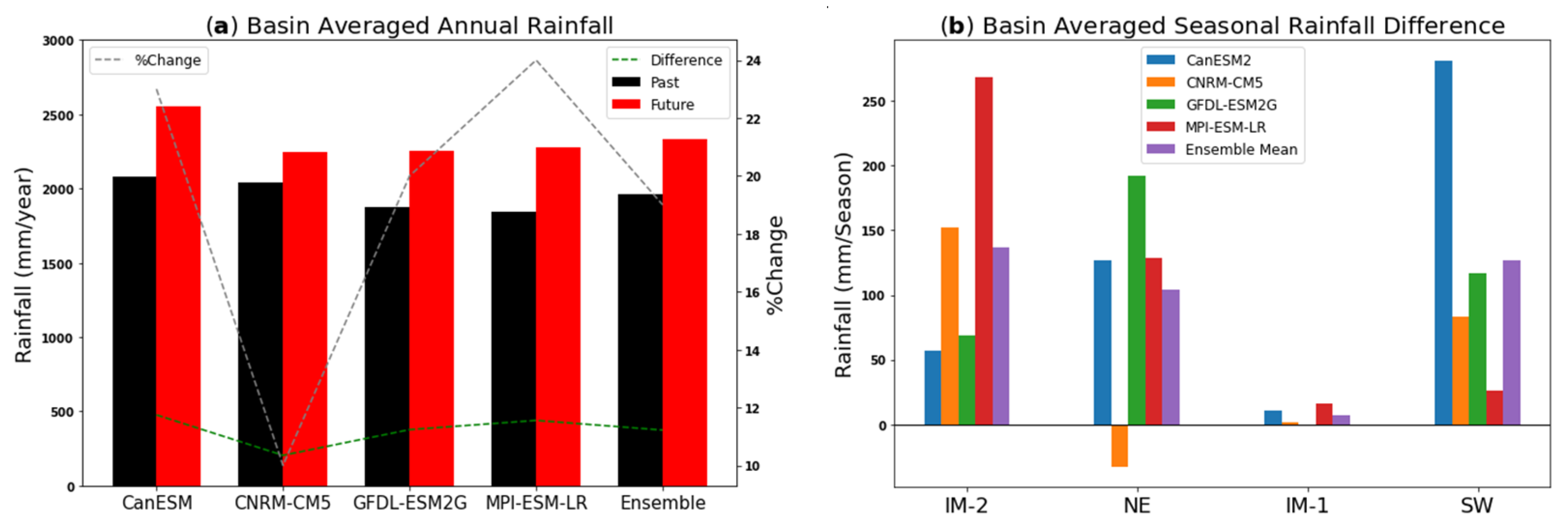
6.1.2. Changes in Annual Climatology of Rainfall

The annual average rainfall changes between the past and the future among the selected GCMs were analyzed at the basin scale, and the results are presented in Figure 4a As shown in the figure, all models show an increasing trend in basin average rainfall; hence, it is very likely that the future climate will experience more rainfall than the past climate. The rainfall is projected to increase by about 19% (~370 mm/year) in the future. Moreover, CanESM2, GFDL-ESM2G, and MPI-ESM-LR show higher rainfall increase rates (23%, 20%, and 24%, respectively) due to higher warming rates, whereas CNRM-CM5 show a lower increase rate (10%) due to a lower warming rate (Figure 3). A similar study conducted in India, another Asian monsoon region country, by Chaturvedi et al. (2012) [48,49] confirmed a future increase in all-India mean precipitation, under the business-as-usual scenario, due to the increased warming effect.
As stated earlier, rainfall in Sri Lanka is influenced mainly by seasonally varying monsoon systems and their interactions with the island’s topography, and thus the elevated regions receive more rainfall. Figure 5a–e compares the spatial distribution of changes in annual average rainfall for the GCMs and their ensemble mean. All four models indicate that the southern hilly region of MRB will very likely receive more rainfall in the upstream area under the future warmer climate.
Besides, it is also important to note that the spatial changes of rainfall projected by CNRM-CM5 will take place at a much lower rate than those projected by the other models, as it projected a lower warming rate (Figure 3b).

6.1.3. Changes in Seasonal Climatology of Rainfall

To understand the seasonal changes in rainfall, the spatial distribution of seasonal climatology differences was calculated and is shown in Figure 6. The basin average seasonal rainfall changes are shown in Figure 4b. Rainfall changes during two major seasons (i.e., NE, and SW monsoons) will be discussed first. As shown in Figure 6b1–b5, during the NE monsoon, three models except for CNRM-CM5 project an increase in rainfall, and the basin average changes are ~100–200 mm more or less uniformly throughout the basin.
The exceptional reduction in the rainfall projected by CNRM-CM5 will be discussed in the next paragraph. During the SW monsoon (Figure 4b), all the model-projected rainfall increases (~25–300 mm) in the future climate, with CanESM2 showing the largest increase and MPI-ESM-LR showing the smallest increase in the basin average rainfall. As for the spatial distributions during this season (Figure 6d1–d5), all models other than MPI-ESM-LR show a higher rainfall increase in the hilly region compared to the downstream region. Therefore, it is likely that both NE and SW monsoon seasons will bring a considerable amount of rainfall in the warmed future climate. The investigation on the other two seasons (i.e., IM-2 and IM-1) showed that during the IM-2 season, it is very likely that rainfall will increase as all the models projected a rainfall increase in the warming climate throughout the basin (Figure 6a1–a5). Among the other models, MPI-ESM-LR predicted the largest rainfall increase in the uppermost and middle regions of the basin during the IM-2 season. On the other hand, the IM-1 season, which brings less rainfall to the basin, will cause no change or a slight increase in basin average rainfall (Figure 4b); however, the distribution map (Figure 6c1–c5) reveals no clear clues on the location of the changes. In general, from the beginning of May (i.e., the onset of the SW monsoon) through the IM-2 season (October and November) until the withdrawal of the NE monsoon (i.e., February), the seasonal rainfall will increase in the future climate.
To investigate exceptional reductions in the rainfall projected by CNRM-CM5 during the NE monsoon and by MPI-ESM-LR during the SW monsoon, weather variables that influence the rainfall mechanism over the island, such as geopotential height, specific humidity, and wind speed, were analyzed at the 850 hPa level. The basin averaged values of each variable for the NE and SW monsoon seasons are given in Figure 7. As shown in Figure 7a1,a2, the geopotential height will increase in the future climate due to increases in temperature in all the models for both seasons. In the case of the reduction in the rainfall projected by CNRM-CM5 during the NE monsoon, the wind speeds projected by all the models show a reduction in its strength Figure 7c1, which indicates that the weaker wind may not be a reason. However, as shown in Figure 7b1, all the models show an increase in the specific humidity except CNRM-CM5, which shows a marginal reduction in this variable. Therefore, the reduction in the rainfall projected in the future climate by CNRM-CM5 could be caused by a marginal reduction in the specific humidity during the NE monsoon. In the case of the rainfall reduction by MPI-ESM-LR during the SW monsoon, no deference is observed in either geopotential height Figure 7a2 or specific humidity (Figure 7b2) from MPI-ESM-LR. Although there is almost no change in wind speed (Figure 7c2) during the SW monsoon, this will not be a reason, as other models show mixed responses despite still showing an increase in rainfall. The reason why MPI-ESM-LR shows less rainfall during the SW monsoon could be related to model physics and parametrizations and their interaction with misrepresentation of topographical features, which needs further investigation.

6.1.4. Extreme Event Data Analysis: Meteorological Rainfall Extremes and Droughts

Rainfall extremes were investigated based on the anomalies of climate indices of consecutive wet/dry days for the past and future basin average rainfall outputs of GCMs. The consecutive wet days (CWD) index is defined as the consecutive number of days during a year with daily rainfall higher than 0.05 mm/day, while the consecutive dry days (CDD) index is defined as the consecutive number of days during a year with daily rainfall of less than 0.05 mm/day. Zhang et al. (2012) [50] also introduced a similar definition. The anomaly is defined as the departure for a year from the climatological averages of CWD and CCD. The positive anomaly values were rank-ordered and plotted against the ranks in Figure 8.
Figure 8a1–e1 shows the anomalies of CWD for observed rainfall (near past: 1997–2017, far past: 1976–1996) and the projected rainfall by the four selected GCMs. Figure 8a1 shows a clear increase in anomalies of CWD observed during the near past period compared to the far past period. As depicted in Figure 8b1–e1, CanESM2, CNRM-CM5, and GFDL-ESM2G show a clear increment in CWD in the future, whereas MPI-ESM-LR shows an increment in most extreme anomalies but a reduction for the other cases of CWD. Therefore, it is likely that future annual wet days will increase under the warming climate.
Similarly, the anomalies of annual CDDs for observation and each GCM are shown in Figure 8a2–e2. A clear increment in anomalies of CDD is also observed for the near past period compared to the far past period (Figure 8a2). As shown in Figure 8b2–e2, CanESM2, CNRM-CM5, and GFDL-ESM2G show a clear increment in CDD in the future, while MPI-ESM-LR shows a reduction in most extreme anomalies but an increase in the other cases of CDD. Therefore, it is likely that future annual dry days will increase under the warming climate.

6.2. WEB-RRI Model Calibration and Validation

The WEB-RRI model was developed to model the hydrological responses of a basin to the past and future climate. The model was calibrated at the Peradeniya discharge location (Figure 2c), using the observed discharge data from 1981 to 1982, which corresponds to the period prior to the Kotmale Dam construction and its operation since 1985. The calibrated model satisfactorily reproduced the base flow and the peak flood with NSE equal to 0.84, MBE equal to 0.91 m3/s, and RMSE equal to 24.48 m3/s (Figure 9a). Subsequently, as shown in Table 3, the calibrated parameters were validated at the same discharge location for the period from 2005 to 2015 with the dam effect (dam operation data are obtained from Mahaweli Authority). During the validation period, the model-simulated discharge at the Peradeniya location was compared to the observed discharge. During the validation period, the model performance indices were NSE equal to 0.77, MBE equal to −1.49 m3/s, and RMSE equal to 4.52 m3/s (Figure 9b). Mainly, the low flow during the dry period, the flow just before the flood onset, the peak flood discharge, and the exact timing of these events were represented satisfactorily during both calibration and validation periods.

6.3. Hydrological Assessment

The WEB-RRI model simulated the natural flow conditions of the basin without considering any dam effects, as long-term data on dam effects are not available for the past and future study periods. The seasonal averages of the simulated river discharges and hydrological extremes of flood and drought events were investigated at the downstream confluence point, the Mannampitiya discharge location (Figure 2c). The all-time maximum inundation depth at each grid cell for both climates was calculated and used to make spatially distributed inundation maps, which were then used for damage assessment.

6.3.1. Discharge Analysis

The past and future annual average discharges and seasonal average discharge differences are shown in Figure 10a,b. Clear increasing signals are observed during the three seasons (i.e., IM2, NE, and SW monsoons), indicating that the basin will yield a higher amount of flow at the discharge location in the future. The approximate range of increments will be ~16.3 m3/s–149.0 m3/s for IM-2, ~3.4 m3/s−107.1 m3/s for the NE monsoon, and 7.0 m3/s ~35.3 m3/s for the SW monsoon in the future climate. During IM-1, except for MPI-ESM-LR, the other three models projected a decrease in flow rate −10.8 m3/s ~23.8 m3/s. Therefore, it is very likely that the discharge will increase in the future during the NE, SW, and IM- 2 seasons, and it is also likely to project a reduction in discharge during the IM-1 season. Consequently, the estimated annual average discharge is very likely to increase in the future climate, and the values may range from ~11 m3/s to 57 m3/s as the percentage changes in the range of 4–24%.

6.3.2. Extreme Event Data Analysis: Hydrological Floods and Droughts

Hydrological extremes are investigated in this section. The daily average discharge simulated for the past and future climates were rank-ordered, and the first 20 peak discharges were analyzed for extreme floods, and the last 20 low flows were analyzed for droughts.
Figure 11a1–d1 shows the first 20 peak discharges estimated by the WEB-RRI model for the inputs from CanESM2, CNRM-CM5, GFDL-ESM2G, and MPI-ESM-LR, respectively. As shown in the figures, the projected future peak discharges are significantly higher in CanESM2 and MPI-ESM-LR and marginally higher in the other two models. Therefore, peak discharges are very likely to increase in the future; thus, hydrological floods are very likely to increase in the future climate in this basin. Similar findings were reported in the Assessment Report 5 of the IPCC, explaining that GCMs have projected the impacts associated with increased flooding with high confidence in the case of small islands [51].
Figure 11a2–d2 shows the last 20 low-flow events for the selected model for both climates. CanESM2 and MPI-ESM-LR project a similar pattern of nearly no change in the future low flow; however, CNRM-CM5 and GFDL-ESM2G project an increase in the future low flow. Therefore, the trend in future hydrological droughts is uncertain, and thus, a firm conclusion cannot be attained based on the GCM projections. Similar findings were reported in the Assessment Report 5 of the IPCC that the overall global scale sign of drought trends has been assessed with low confidence except for the high confidence projections of increased droughts in some regions of the world [51]. This low confidence level of GCMs in projecting future droughts could be an arguable reason for the observed uncertainty in projected hydrological droughts.

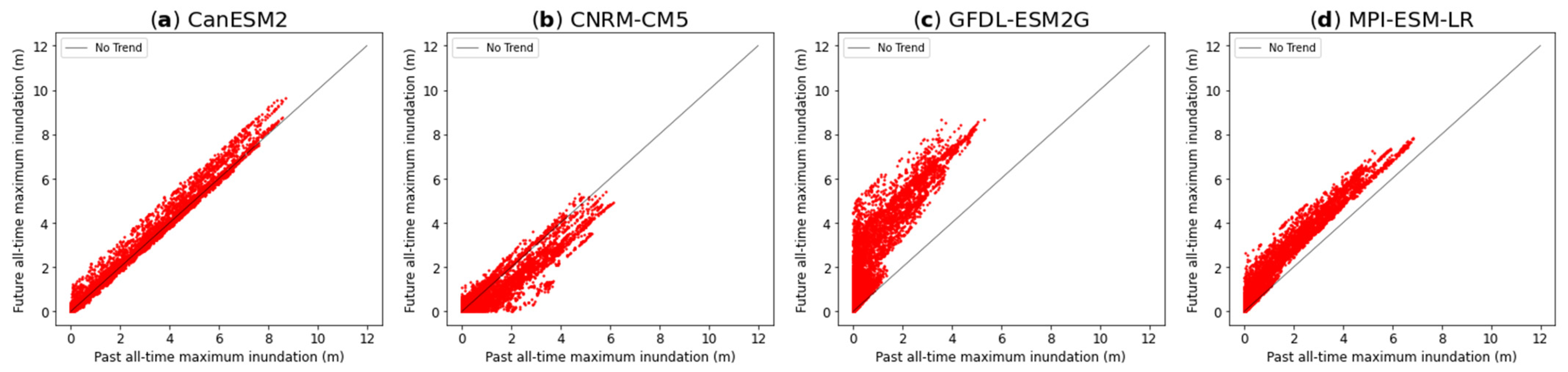
6.3.3. Inundation Analysis

The difference between past and future climates in all-time maximum inundation depth at each grid cell was estimated from the WEB-RRI simulated inundation gridded data for each GCM individually and is plotted in Figure 12b1–b4, and the past all-time inundation depth gridded data are given in Figure 12a1–a4 for reference. As shown in the figure, except for the CNRM-CM5 model, the other three models project an increase in the inundation extent for all-time flood depth. Therefore, it is likely that the flood inundation area and risk will increase in the basin under the future climate. The contrasting behaviour of CNRM-CM5 can be attributed to the reduction in future rainfall due to a low warming rate and the reduction in rainfall during the NE monsoon, which brings a considerable amount of rainfall to the downstream area of the basin. To verify the simulation results further, the all-time seasonal (i.e., NE monsoon) maximum inundation depths simulated by the WEB-RRI model were estimated. Figure 13 shows the scatter plot of past versus future all-time seasonal maximum inundation depths during the NE monsoon for all the model grids. As shown in the figure, CNRM-CM5 projects a decrease in all-time seasonal inundation depth in the future climate compared with those in the past climate during the NE monsoon, whereas the other three models project clear increases in the future inundation depth. Therefore, this contrasting behaviour of a decreased inundation depth from CNRM-CM5 is due to uncertainties in rainfall projections during the NE monsoon season.

6.3.4. Socio-Economic Damage Analysis

To understand the impact of climate change on the socio-economic features, the population data and land cover data were set into layers in GEE. Additionally, the past and future simulated inundation over 1 m in depth from WEB-RRI has been overlaid for each selected GCM, and the statistics of inundated population, cropland and urban area were extracted for analysis, as shown in Figure 14. The following results were obtained from the analyses: (a) it is very likely that flood damage to the population will increase; (b) it is likely that damage to the cropland will increase; and (c) inundation of urban area will likely increase in the future.

6.3.5. Decision Making

Policymakers can utilize the qualitative level of confidence based on Table 4 (basin-scale annual assessments) and Table 5 (seasonal discharge) to make decisions for disaster risk reduction. Information on an increasing level of confidence of extreme rainfall and hydrological floods is an indication of future increases in disasters and water resources. Policymakers could react in two directions by implementing soft or hard countermeasures: one is to mitigate disasters, and the other is to utilize water resources or opportunities brought by disasters for effective planning. On the other hand, the increasing level of confidence in meteorological droughts shows a possible water shortage in the future climate. Policymakers should strategically plan drought monitoring and mitigation to handle water shortage to reduce future risks. Further, decision-makers can decide to either implement new countermeasures or continue the current disaster management practices under an uncertain level of confidence.

7. Conclusions

This paper presents an integrated approach for assessing climate change impacts on the hydro-meteorological characteristics of river basins. The assessment is accomplished by selecting reliable GCMs based on their regional performances, identifying climate change signals, clarifying uncertainties from the selected GCMs, developing a WEB-RRI model to simulate the basin hydrological responses of floods and droughts seamlessly under climate change, and then facilitating decision-making procedures.
The proposed approach has been applied to MRB in Sri Lanka to assess the impacts of climate change on water resources. The GCM selection procedure found that four GCMs (CanESM2, CNRM-CM5, GFDL-ESM2G, and MPI-ESM-LR) out of 44 were capable of satisfactorily simulating the past regional climate. As a result, these models’ precipitation and temperature data were obtained and statistically bias-corrected. The bias-corrected results showed that the basin average annual temperature is very likely to increase in the future, on average with a future temperature increase of 1.1 °C over the future 20 years. Under this warming future climate, the future annual rainfall over the basin is very likely to increase, and the range will vary from 204 to 476 mm/year. The extreme event analysis showed that future heavy rainfall and meteorological droughts are likely to increase at the basin scale annually as three out of the four models showed an increase in future anomalies of CWD in terms of heavy rainfall and an increase in future anomalies of CDD concerning meteorological droughts. On the other hand, the future annual average discharge at the Mannampitiya gauging station is very likely to increase, and the range of increase will vary from 11 m3/s to 57 m3/s. The extreme flood event analysis showed that the hydrological floods are very likely to increase according to the first 20 peak flows in the future climate. Meanwhile, the last 20 low flow rates indicated that the trend of future hydrological droughts is uncertain. Moreover, the mapping of the all-time maximum inundation depth of more than 1 m showed that the future inundated population, cropland, and the urban land area will likely increase. Therefore, there will be more economic damage due to floods in the future under the changing climate.
It is to be noted that the statistical bias correction does not represent the spatial and temporal connectivity; however, it is useful to identify the range of target parameters from the selected GCMs with less computational effort. To overcome the limitations of the statistical approach, the dynamical downscaling method can be used to obtain quantitative outputs, representing the spatial and temporal connectivity for designing infrastructure development at the local scale. Therefore, future research will focus on quantitative analysis to represent the spatial and temporal connectivity based on the dynamical downscaling approach for supporting local-scale future infrastructure development and the identification of hazard.

Author Contributions

H.S., T.K. and M.R. conceived and formulated the research. H.S., M.R. and L.Z. performed the calculation, simulation, analysis, and assessments. K.T., A.Y. and M.K. contributed to climate data processing in terms of model selection and bias correction with DIAS. H.S., T.K. and M.R. wrote the paper, with H.S. as the lead author. All authors have read and agreed to the published version of the manuscript.

Funding

This research received no external funding.

Institutional Review Board Statement

Not applicable.

Informed Consent Statement

Not applicable.

Data Availability Statement

All the GCM data used in this study are openly available in DIAS at https://diasjp.net/en/service/cmip5/ (accessed on 14 August 2019). The observed rainfall used for bias correction in this study is also available in DIAS.

Acknowledgments

We thank the government of Sri Lanka, JICA, GRIPS, ICHARM, and PWRI in Japan for supporting this research. Special thanks to the University of Tokyo (DIAS, I.No: JPMXD-0716808999) for providing IPCC/AR5-CMIP5 climate dataset. We also thank MASL, DOI-SL, DOM-SL, NASA, FAO, and JMA for providing data needed for hydrological model development and validation. We thank Okubo Masahiko for his English editing contribution. We also acknowledge anonymous reviewers for their comments and suggestions that improved this manuscript.

Conflicts of Interest

The authors declare no conflict of interest.

References

  1. Roxburgh, T.; Elli, K.; Johnson, J.A.; Baldos, U.L.; Hertel, T.; Nootenboom, C.; Polasky, S. Global Futures: Assesing the Global Economic Impacts of Environmental Change to Support Policy-Making; Summary Report; WWF: Gland, Switzerland, 2020. [Google Scholar]
  2. UN Water. Policy Brief Climate Change and Water; UN Water: Geneva, Switzerland, 2019; pp. 1–8. [Google Scholar]
  3. Teng, J.; Vaze, J.; Chiew, F.H.S.; Wang, B.; Perraud, J.M. Estimating the relative uncertainties sourced from GCMs and hydrological models in modeling climate change impact on runoff. J. Hydrometeorol. 2012, 13, 122–139. [Google Scholar] [CrossRef]
  4. CREED. The Human Cost of Water Related Disasters; CREED: Brasschaat, Belgium, 2015. [Google Scholar]
  5. Kumar, A.; Sharma, M.P. A modeling approach to assess the greenhouse gas risk in Koteshwar hydropower reservoir, India. Hum. Ecol. Risk Assess. 2016, 22, 1651–1664. [Google Scholar] [CrossRef]
  6. Kumar, A.; Sharma, M.P. Assessment of risk of GHG emissions from Tehri hydropower reservoir, India. Hum. Ecol. Risk Assess. 2016, 22, 71–85. [Google Scholar] [CrossRef]
  7. UN. Sendai Framework for Disaster Risk Reduction: 2015–2030; UN: New York, NY, USA, 2015. [Google Scholar]
  8. UN-Secretary-General. ECOSOC–Economic and Social Council: Special Edition: Progress towards the Sustainable Development Goals; UN: New York, NY, USA, 2019. [Google Scholar]
  9. UN. Adoption of the Paris Agreement Proposal by the President; UN: New York, NY, USA, 2015. [Google Scholar]
  10. Zhou, L.; Rasmy, M.; Takeuchi, K.; Koike, T.; Selvarajah, H.; Ao, T. Adequacy of Near Real-Time Satellite Precipitation Products in Driving Flood Discharge Simulation in the Fuji River Basin, Japan. Appl. Sci. 2021, 11, 1087. [Google Scholar] [CrossRef]
  11. Koike, T.; Koudelova, P.; Jaranilla-sanchez, P.A.; Bhatti, A.M.; Nyunt, C.T.; Tamagawa, K. River management system development in Asia based on Data Integration and Analysis System (DIAS) under GEOSS. Earth Sci. 2014, 58, 76–95. [Google Scholar] [CrossRef]
  12. Papaioannou, G.; Varlas, G.; Terti, G.; Papadopoulos, A.; Loukas, A.; Panagopoulos, Y.; Dimitriou, E. Flood inundation mapping at ungauged basins using coupled hydrometeorological-hydraulic modelling: The catastrophic case of the 2006 Flash Flood in Volos City, Greece. Water 2019, 11, 2328. [Google Scholar] [CrossRef] [Green Version]
  13. Bralower, T.; Bice, D. Earth in the Future. Understanding GCMs. 2018. Available online: https://www.e-education.psu.edu/earth103/node/607 (accessed on 4 April 2020).
  14. Freer, J.; Beven, K.J.; Neal, J.; Schumann, G.; Hall, J.; Bates, P. Flood Risk and Uncertainty; Cambridge University Press: Cambridge, UK, 2013; Volume 9781107006. [Google Scholar]
  15. Nyunt, C.T.; Koike, T.; Yamamoto, A. Statistical bias correction for climate change impact on the basin scale precipitation in Sri Lanka, Philippines, Japan and Tunisia. Hydrol. Earth Syst. Sci. Discuss. 2016, 14, 1–32. [Google Scholar]
  16. Rasmy, M.; Koike, T.; Lawford, P.; Hara, M. Assessment of future water resources in the tone river basin using a combined dynamical-stastical downscaling approach. J. Jpn. Soc. Civ. Eng. Ser. B1 (Hydraul. Eng.) 2015, 71, 73–78. [Google Scholar]
  17. Kawasaki, A.; Yamamoto, A.; Koudelova, P.; Acierto, R.; Nemoto, T.; Kitsuregawa, M.; Koike, T. Data integration and analysis system (DIAS) contributing to climate change analysis and disaster risk reduction. Data Sci. J. 2017, 16, 41. [Google Scholar] [CrossRef] [Green Version]
  18. Zhang, L.E.I.; Xu, Y.; Meng, C.; Li, X.; Liu, H.; Wang, C. Comparison of statistical and dynamic downscaling techniques in generating high-resolution temperatures in China from CMIP5 GCMs. J. Appl. Meteorol. Climatol. 2020, 59, 207–235. [Google Scholar] [CrossRef]
  19. Maurer, E.P.; Hidalgo, H.G. Utility of daily vs. monthly large-scale climate data: An intercomparison of two statistical downscaling methods. Hydrol. Earth Syst. Sci. 2008, 12, 551–563. [Google Scholar] [CrossRef] [Green Version]
  20. Tang, J.; Niu, X.; Wang, S.; Gao, H.; Wang, X.; Wu, J. Statistical downscaling and dynamical downscaling of regional climate in China: Present climate evaluations and future climate projections. J. Geophys. Res. Atmos. 2016, 121, 2110–2129. [Google Scholar] [CrossRef] [Green Version]
  21. Shrestha, M.; Aranilla-Sanchez, P.A.; Wang, L.; Koike, T. Investigating the Hydrologic Response of Current Dam Operation System To Future Climate in a Snowy River Basin (Yattajima) of Japan. J. Jpn. Soc. Civ. Eng. Ser. B1 2015, 71, I_103–I_108. [Google Scholar] [CrossRef] [Green Version]
  22. Rasmy, M.; Sayama, T.; Koike, T. Development of water and energy Budget-based Rainfall-Runoff -Inundation model (WEB-RRI) and its veri fi cation in the Kalu and Mundeni River Basins, Sri Lanka. J. Hydrol. 2019, 579, 124163. [Google Scholar] [CrossRef]
  23. IPCC. Summary for Policymakers. In Climate Change 2013: The Physical Science Basis. Contribution of Working Group I to the Fifth Assessment Report of the Intergovernmental Panel on Climate Change; Stocker, T.F., Qin, D., Plattner, G.-K., Tignor, M., Allen, S.K., Boschung, J., Eds.; Cambridge University Press: Cambridge, UK, 2013. [Google Scholar]
  24. UNDRR. DesInventar Sendai. 2020. Available online: https://www.desinventar.net/DesInventar/profiletab.jsp (accessed on 1 April 2021).
  25. DOM-SL. Climate of Sri Lanka. 2020. Available online: http://www.meteo.gov.lk/index.php?option=com_content&view=article&id=94&Itemid=310&lang=en#4-northeast-monsoon-season-december-february (accessed on 4 April 2020).
  26. DOA-SL. Agro Climatic Zones. 2020. Available online: https://www.doa.gov.lk/index.php/en/weather-climate (accessed on 4 May 2020).
  27. CEB-SL. Annual Report 2015; CEB-SL: Colombo, Sri Lanka, 2017.
  28. MASL-SL. Mahaweli Authority of Sri Lanka. In Proceedings of the GEOS Asia Pacific Symposium, Kyoto, Japan, 24–26 October 2018. [Google Scholar]
  29. Suzuki-Parker, A.; Kusaka, H.; Takayabu, I.; Dairaku, K.; Ishizaki, N.N.; Ham, S. Contributions of GCM/RCM uncertainty in ensemble dynamical downscaling for precipitation in East Asian summer monsoon season. Sci. Online Lett. Atmos. 2018, 14, 97–104. [Google Scholar] [CrossRef]
  30. van Vuuren, D.P.; Edmonds, J.; Kainuma, M.; Riahi, K.; Thomson, A.; Hibbard, K.; Hurtt, G.C.; Kram, T.; Krey, V.; Lamarque, J.-F.; et al. The representative concentration pathways: An overview. Clim. Chang. 2011, 109, 5–31. [Google Scholar] [CrossRef]
  31. Stefanidis, K.; Panagopoulos, Y.; Mimikou, M. Response of a multi-stressed Mediterranean river to future climate and socio-economic scenarios. Sci. Total Environ. 2018, 627, 756–769. [Google Scholar] [CrossRef]
  32. Sellers, P.J.; Tucker, C.J.; Collatz, G.J.; Los, S.O.; Justice, C.O.; Dazlich, D.A.; Randall, D.A. A Revised Land Surface Parameterization (SiB2) for Atmospheric GCMs. Part II: The Generation of Global Fields of Terrestrial Biophysical Parameters from Satellite Data. J. Clim. 1996, 9, 706–737. [Google Scholar] [CrossRef] [Green Version]
  33. Wang, L.; Koike, T.; Yang, K.; Jackson, T.J.; Bindlish, R.; Yang, D. Development of a distributed biosphere hydrological model and its evaluation with the Southern Great Plains experiments (SGP97 and SGP99). J. Geophys. Res. Atmos. 2009, 114, 1–15. [Google Scholar] [CrossRef] [Green Version]
  34. Sayama, T.; Ozawa, G.; Kawakami, T.; Nabesaka, S.; Fukami, K. Rainfall–runoff–inundation analysis of the 2010 Pakistan flood in the Kabul River basin. Hydrol. Sci. J. 2012, 57, 298–312. [Google Scholar] [CrossRef]
  35. PBrunner; Simmons, C.T.; Cook, P.G.; Therrien, R. Modeling surface water-groundwater interaction with MODFLOW: Some considerations. Ground Water 2010, 48, 174–180. [Google Scholar]
  36. Adler, R.F.; Huffman, G.J.; Chang, A.; Ferraro, R.; Xie, P.-P.; Janowiak, J.; Rudolf, B.; Schneider, U.; Curtis, S.; Bolvin, D.; et al. The version-2 global precipitation climatology project (GPCP) monthly precipitation analysis (1979-present). J. Hydrometeorol. 2003, 4, 1147–1167. [Google Scholar] [CrossRef]
  37. Liebmann, B.; Smith, C.A. Description of a complete (interpolated) outgoing longwave radiation dataset. Bull. Amer. Meteor. Soc. 1996, 77, 1275–1277. [Google Scholar]
  38. Rayner, N.A.; Parker, D.E.; Horton, E.B.; Folland, C.K.; Alexander, L.V.; Rowell, D.P.; Kent, E.C.; Kaplan, A. Global analyses of sea surface temperature, sea ice, and night marine air temperature since the late nineteenth century. J. Geophys. Res. Atmos. 2003, 108, 4407. [Google Scholar] [CrossRef]
  39. Kobayashi, S.; Ota, Y.; Harada, Y.; Ebita, A.; Moriya, M.; Onoda, H.; Onogi, K.; Kamahori, H.; Kobayashi, C.; Endo, H.; et al. The JRA-55 reanalysis: General specifications and basic characteristics. J. Meteorol. Soc. Jpn. 2015, 93, 5–48. [Google Scholar] [CrossRef] [Green Version]
  40. Sahu, N.; Yamashika, Y.; Takara, K. Impact Assessment of IOD/ENSO in the Asian Region; Annuals of Disaster Prevention Research Institute, Kyoto University: Kyoto, Japan, 2010. [Google Scholar]
  41. Breeick, S. NASA: Earth Data Powered by EOSDIS. 2020. Available online: https://earthdata.nasa.gov/ (accessed on 4 May 2020).
  42. Afifi, Z.; Chu, H.J.; Kuo, Y.L.; Hsu, Y.C.; Wong, H.K.; Ali, M.Z. Residential flood loss assessment and risk mapping from high-resolution simulation. Water 2019, 11, 751. [Google Scholar] [CrossRef] [Green Version]
  43. Kiczko, A.; Mirosław-Światek, D. Impact of uncertainty of floodplain Digital Terrain Model on 1D hydrodynamic flow calculation. Water 2018, 10, 1308. [Google Scholar] [CrossRef] [Green Version]
  44. Zhu, X.; Dai, Q.; Han, D.; Zhuo, L.; Zhu, S.; Zhang, S. Modeling the high-resolution dynamic exposure to flooding in a city region. Hydrol. Earth Syst. Sci. 2019, 23, 3353–3372. [Google Scholar] [CrossRef] [Green Version]
  45. European-Commission. GHS Population Grid, Derived from GPW4, Multitemporal (1975, 1990, 2000, 2015). 2015. Available online: https://developers.google.com/earth-engine/datasets/catalog/JRC_GHSL_P2016_POP_GPW_GLOBE_V1#bands (accessed on 25 November 2020).
  46. Friedl, M.; Sulla-Menashe, D. MCD12Q1 MODIS/Terra+Aqua Land Cover Type Yearly L3 Global 500m SIN Grid V006. NASA EOSDIS Land Processes DAAC, 2019. Available online: https://doi.org/10.5067/MODIS/MCD12Q1.006 (accessed on 25 November 2020).
  47. Nash, J.E.; Sutcliffe, J.V. River flow forecasting through conceptual models: Part I-A discussion of principles. J. Hydrol. 1970, 10, 282–290. [Google Scholar] [CrossRef]
  48. Chaturvedi, R.K.; Joshi, J.; Jayaraman, M.; Bala, G.; Ravindranath, N.H. Multi-model climate change projections for India under representative concentration pathways. Curr. Sci. 2012, 103, 791–802. [Google Scholar]
  49. Christensen, J.H.; Aldrian, E.; An, S., II; Cavalcanti, I.F.A.; de Castro, M.; Dong, W.; Goswami, P.; Hall, A.; Kanyanga, J.K.; Kitoh, A.; et al. Climate phenomena and their relevance for future regional climate change. In Climate Change 2013: The Physical Sci-ence Basis. Contribution of Working Group I to the Fifth Assessment Report of the Intergovernmental Panel on Climate Change; Cambridge University Press: Cambridge, UK, 2013; Volume 9781107057, pp. 1217–1308. [Google Scholar]
  50. Zhang, Y.; Jiang, F.; Wei, W.; Liu, M.; Wang, W.; Bai, L.; Li, X.; Wang, S. Changes in annual maximum number of consecutive dry and wet days during 1961-2008 in Xinjiang, China. Nat. Hazards Earth Syst. Sci. 2012, 12, 1353–1365. [Google Scholar] [CrossRef]
  51. Masson-Delmotte, V.; Zhai, P.; Pörtner, H.-O.; Roberts, D.; Skea, J.; Shukla, P.R.; Pirani, A.; Moufouma-Okia, W.; Péan, C.; Pidcock, R.; et al. Impacts of 1.5 °C global warming on natural and human systems. In Global Warming of 1.5 °C. An IPCC Special Report on the Impacts of Global Warming of 1.5 °C above Preindustrial Levels and Related Global Greenhouse Gas Emission Pathways [...]; IPCC: Geneva, Switzerland, 2018. [Google Scholar]
Figure 1. Research framework.
Water 13 01218 g001
Figure 2. (a) Topographical map of Sri Lanka with the demarcation of the Mahaweli River basin, (b) topography of the Mahaweli River basin, (c) land use with distribution of discharge measurement points, and (d) demarcation of climatic zones with rain gauge network.
Water 13 01218 g002
Figure 3. Basin average temperature difference (future—past): (a) bar plot for monthly changes; and (b) box-and-whisker plot for annual changes.
Water 13 01218 g003
Figure 4. (a) The comparison of basin average annual rainfall (mm/year) between past and future climate and percentage changes (%) for each selected GCM; and (b) basin average seasonal rainfall differences (future—past) for selected GCMs and the ensemble mean.
Water 13 01218 g004
Figure 5. The comparison of annual average rainfall differences (future—past) in mm/year for the selected models (ad) and the ensemble mean (e).
Water 13 01218 g005
Figure 6. The comparison of seasonal average rainfall differences (future—past) for the selected models: CanESM2 (a1d1), CNRM-CM5 (a2d2), GFDL-ESM2G (a3d3), MPI-ESM-LR (a4d4) and the ensemble mean (a5d5).
Water 13 01218 g006
Figure 7. The comparisons of past and future climate seasonal average of variables influencing rainfall: (a1,2) geopotential height, (b1,2) specific humidity, and (c1,2) wind speed.
Water 13 01218 g007
Figure 8. Anomalies of CWD and CDD of observed far past (1976–1996) and near past (1997–2017) rainfall and the past and future rainfall of the selected models: Observed Rainfall (a1,2), CanESM2 (b1,2), CNRM-CM5 (c1,2), GFDL-ESM2G (d1,2), MPI-ESM-LR (e1,2).
Water 13 01218 g008
Figure 9. Comparison between observed discharge and simulated discharge: (a) model calibration for 1981–1982 under the natural river flow; and (b) model validation for 2005 to 2015 with dam operations.
Water 13 01218 g009
Figure 10. (a) Annual average discharge at Mannampitiya gauging station of the selected models; and (b) seasonal average discharge difference at Mannampitiya gauging station of the selected models.
Water 13 01218 g010
Figure 11. First 20 peak-flow events and the last 20 low-flow events of daily average discharge values of the past and future 20 years of the selected GCMs: CanESM2 (a1,2), CNRM-CM5 (b1,2), GFDL-ESM2G (c1,2), MPI-ESM-LR (d1,2).
Water 13 01218 g011
Figure 12. (a) Past all-time inundation depth; and (b) inundation depth deference between future and past of the selected GCMs: CanESM2 (a1,b1), CNRM-CM5 (a2,b2), GFDL-ESM2G (a3,b3), MPI-ESM-LR (a4,b4).
Water 13 01218 g012
Figure 13. Past vs. future all-time seasonal maximum inundation during the NE monsoon of the selected GCMs (ad).
Water 13 01218 g013
Figure 14. Socio-economic damage assessment.
Water 13 01218 g014
Table 1. Model selection summary for annual, SW monsoon, and NE monsoon period average.
Model NameInstituteCountryAnnualSW MonsoonNE MonsoonGrand Total *Remarks
PrecipitationTotal IndexPrecipitationTotal IndexPrecipitationTotal Index
ACCESS1.0CSIRO-BOMAustralia04160313PPR
ACCESS1.3CSIRO-BOMAustralia−1−3−1−3−13−3
BCC-CSM1.1BCCChina−1−1−12012
BCC-CSM1.1(m)BCCChina0−20−301−4
BNU-ESMBNUChina1311115
CanCM4CCCMACanada15151414FF
CanESM2CCCMACanada16150213Selected
CCSM4NCARUSA1314−107
CESM1(BGC)NCARUSA1315019
CESM1(CAM5)NCARUSA1516−1011
CESM1(FASTCHEM)NCARUSA1−113−102
CESM1(WACCM)NCARUSA1610−139
CMCC-CESMCMCCItaly−13−151210
CMCC-CMSCMCCItaly−13−140310
CNRM-CM5NCMRFrance16151415Selected
CNRM-CM5-2NCMRFrance04031310
CSIRO-Mk3.6.0CSIRO-QCCCEAustralia−1−1−1−101−1
FGOALS-g2LASG-CESSChina0−10−110−2
FIO-ESMFIOChina1213−1−14
GFDL-CM2.1NOAA-GFDLUSA14171516FF
GFDL-CM3NOAA-GFDLUSA1416−1010
GFDL-ESM2GNOAA-GFDLUSA15161213Selected
GFDL-ESM2MNOAA-GFDLUSA1112136
GISS-E2-HNASA-GISSUSA−1−2−1−202−2
GISS-E2-H-CCNASA-GISSUSA−10−1−2031
GISS-E2-RNASA-GISSUSA−10−1−1054
GISS-E2-R-CCNASA-GISSUSA−12−1−1034
HadCM3MOHCUK−1002011
HadGEM2-ESMOHCUK−1002157
INM-CM4INMRussia0−2110−1−2
IPSL-CM5A-LRIPSLFrance0−20−3−1−4−9
IPSL-CM5A-MRIPSLFrance0−1000−2−3
IPSL-CM5B-LRIPSLFrance−1−4−1−4−10−8
MIROC-ESMUTJapan0−3−1−400−7
MIROC-ESM-CHEMUTJapan0−2−1−30−1−6
MIROC4hUTJapan02−10146
MIROC5UTJapan15150212
MPI-ESM-LRMPI-NGermany17171519Selected
MPI-ESM-MRMPI-NGermany16013519PPR
MPI-ESM-PMPI-NGermany17171620FF
MRI-CGCM3MRIJapan−1−2−1−403−3
MRI-ESM1MRIJapan−1−40−5−10−9
NorESM1-MNCCNorway1−112−1−3−2
NorESM1-MENCCNorway10120−10
Grand Total * = Annual Total Index + SW Total Index + NE Total Index. FF = Failed to simulate Future rainfall. PPR = Poor Precipitation Representation in past.
Table 2. Daily rain gauges in the Mahaweli River basin with names, climatic zones, locations, and annual average rainfall in mm.
IDStation NameClimatic ZoneLatitude (N)Longitude (E)Annual Average Rainfall (mm)IDStation NameClimatic ZoneLatitude (N)Longitude (E)Annual Average Rainfall (mm)
1MalibodaWet6.8980.43458217BowatennaIntermediate7.6780.671649
2WatawalaWet6.9580.54514118UlhitiyaDry7.4881.061899
3CalidoniaWet6.9080.70375919EleharaDry7.7380.791812
4AmbewelaWet6.8780.80207120DambuluoyaDry7.8180.541794
5KotmaleWet7.0680.60323721KandalamaDry7.8880.661388
6Peradeniya_IDWet7.2780.61182322Kalawewa RBDry8.0280.541339
7Peradeniya_BotWet7.2780.60191923AngamedillaDry7.8680.911591
8KatugastotaWet7.3280.62178024MaduruoyaDry7.6581.221723
9PolgollaWet7.3280.65180825Para.samudrayaDry7.9181.001572
10BandarawelaIntermediate6.8381.00151926PalugasdamanaDry7.9681.031426
11VictoriaIntermediate7.2480.79146627GirithaleDry8.0080.921364
12RandenigalaIntermediate7.2080.92198728MinneriyaDry8.0380.891258
13RantambeIntermediate7.2080.95172629Kaudulla WewaDry8.1480.931425
14Minipe LBIntermediate7.2180.98164530HuruluwewaDry8.2280.711263
15MapakadawewaIntermediate7.2981.03180031KantaleDry8.3781.001465
16IllukumburaIntermediate7.5480.80252832Alle TankDry8.3781.301315
Table 3. Model-calibrated parameters for the MRB.
ParametersUnitValue
Soil Parameters (basin average)
  Saturated water content (θS)m3/m30.54
  Residual soil water content (θr)m3/m30.07
  Saturated hydraulic conductivity for soil surfacemm/h12.88
  van Genuchten parameter (α)m−20.03
  van Genuchten parameter (n) 1.43
  Soil depth (DS)m1.50
River Parameters
  Manning’s roughness coefficient for river 0.06
  Manning’s roughness coefficient for slope 0.60
  Width parameter (CW) 8.00
  Width parameter (SW) 0.34
  Depth parameter (Cd) 0.90
  Depth parameter (Sd) 0.20
Table 4. Summary of basin-scale annual assessment.
Meteorological Assessment Hydrological Assessment
Future RainfallFuture Extreme RainfallFuture Drought Future DischargeFuture FloodFuture Drought
Level of confidenceVery likely increaseLikely increaseLikely increase Very likely increaseVery likely increase
Table 5. Summary of seasonal discharges at Peradeniya discharge location.
Temporal ScaleLevel of Confidence of Future Discharge
IM-2Very likely increase
NEVery likely increase
IM-1Likely increase
SWVery likely increase
Publisher’s Note: MDPI stays neutral with regard to jurisdictional claims in published maps and institutional affiliations.

