Multi-Spatial Resolution Rainfall-Runoff Modelling—A Case Study of Sabari River Basin, India

Abstract

One of the challenges in rainfall-runoff modeling is the identification of an appropriate model spatial resolution that allows streamflow estimation at customized locations of the river basin. In lumped modeling, spatial resolution is not an issue as spatial variability is not accounted for, whereas in distributed modeling grid or cell resolution can be related to spatial resolution but its application is limited because of its large data requirements. Streamflow estimation at the data-poor customized locations is not possible in lumped modeling, whereas it is challenging in distributed modeling. In this context, semi-distributed modeling offers a solution including model resolution and estimation of streamflow at customized locations of a river basins with less data requirements. In this study, the Hydrologic Engineering Center-Hydrologic Modeling System (HEC-HMS) model is employed in semi-distribution mode on river basins of six different spatial resolutions. The model was calibrated and validated for fifteen and three selected flood events, respectively, of three types, i.e., single peak (SP), double peak (DP)- and multiple peaks (MP) at six different spatial resolution of the Sabari River Basin (SRB), a sub-basin of the Godavari basin, India. Calibrated parameters were analyzed to understand hydrologic parameter variability in the context of spatial resolution and flood event aspects. Streamflow hydrographs were developed, and various verification metrics and model scores were calculated for reference- and calibration- scenarios. During the calibration phase, the median of correlation coefficient and NSE for all 15 events of all six configurations was 0.90 and 0.69, respectively. The estimated streamflow hydrographs from six configurations suggest the model’s ability to simulate the processes efficiently. Parameters obtained from the calibration phase were used to generate an ensemble of streamflow at multiple locations including basin outlet as part of the validation. The estimated ensemble of streamflows appeared to be realistic, and both single-valued and ensemble verification metrics indicated the model’s good performance. The results suggested better performance of lumped modeling followed by the semi-distributed modeling with a finer spatial resolution. Thus, the study demonstrates a method that can be applied for real-time streamflow forecast at interior locations of a basin, which are not necessarily data rich.

1. Introduction

Hydrologic science, including rainfall-runoff modeling, has been an important discipline for several decades because of intriguing science questions and associated socio-economic issues [1,2,3]. Increased data access over a wider area for longer periods, and availability of high computing power in combination with various advanced techniques has allowed hydrologic sciences to evolve over different paradigms, i.e., empiricism, theory, and computational simulation, and now data-intensive sciences [4,5,6]. It enhanced the understanding of rainfall-runoff processes as well as assisted in developing solutions of various aspects ranging from engineering to policy. However, heterogeneity of hydrologic processes in space and time, and unavailability of data either due to a lack of monitoring networks or absence of measurements during extremes make rainfall-runoff modeling still an age-old problem for certain regions and periods of time. In this context, the three decades old effort “Predictions in Ungauged Basins” (PUB) appears to be much very relevant even now [7].

Numerous hydrologic models of different types, e.g., conceptual, physically based and statistical models, have been developed over the years mainly driven by particular study objectives [8,9]. However, a few of them have been widely used and are popular among researchers. Although a model is chosen based on the problem that needs to be solved, i.e., water balance accounting vs. flood modeling, simplicity in model structure, data requirements, informative user manuals and ease of handling dominate the model selection process. When a model is applied in a region, the model structure is typically not disturbed. However, the parameters are modified on the hypothesis that the new values of parameters reflect the heterogeneity of the hydrological processes. Yet, only a few studies explored the model structure approximation of regional hydrology by running multiple hydrological models of different structures [10].

Moreover, the modeling is intricate for the interior basin, which will typically have no or limited data, resulting in a poorer understanding of the processes operating there. Parameter estimation and runoff simulation of basin interior are possible via employing scaling or regionalization or a combination of both techniques. The transfer of parameters from other similar basins is done through the above techniques, and then a model is executed either in lumped- or semi-distributed mode for runoff estimation [11,12,13,14,15,16,17,18,19]. Aside from regionalization technique, another important question is the appropriate spatial resolution for the modeling context. Understanding the role of spatial resolution in the modeling context and insights on parameters of a model helps the transfer of parameters for data-poor regions, including interior locations of a basin.

Several studies have employed different hydrologic models in the semi-distributed mode for different sizes of the basin in urban and rural settings, and then analyzed streamflow for different space- and time-scales; see references in Table 1 of [20]. Contradictory results from several studies, i.e., no significant or both increased and decreased flood peaks were observed for different spatial resolutions [21,22,23,24,25,26,27,28]. Although no conclusive remarks are drawn, the results suggest that the model performance is basin sensitive. Note that the performance is also influenced by several factors, including the type of model and the spatial and temporal resolution of input [10,29]. In this context, modeling becomes more challenging for a real-time forecast system, and both input- and hydrologic uncertainties need to be studied in association with the above mentioned factors including spatial resolution [30,31,32,33,34]. Input uncertainty dominated by rainfall plays a key role in runoff estimation, and significant research has been done on various rainfall aspects including rainfall data resolution [35,36,37]. Apart from it, parametric uncertainty combined (lack) of availability of streamflow at a basin’s interior versus the basin outlet raises concerns on the reliability of parameters [38].

In this context, we pose two questions, i.) Do values of parameters vary with respect to the basin and event aspects? and ii.) Does model performance vary with respect to the spatial resolution? As part of this study, calibrated parameters with respect to the basin area were analyzed. For this, the role of different dominant processes was assumed to vary with basin area. Insights based on the analysis of spatial resolution, parameters and flood event aspects assists in the scientific understanding of regional hydrology as well as in developing a reliable real-time forecast system to issue forecasts at interior locations of the basin.

The Godavari River Basin (GRB) has approximately 140 flow measurement stations, of which 52- and 88-stations measure only the gauge or the gauge and discharge, respectively. Most of the stations are along the main tributary, and stations in the interior of the basins on sub-tributaries are relatively few and they do not have a long period of the record as compared to the main tributary stations. Only a few studies explored the basin in a hydrologic context. Reference [39] showed the application of a hydrologic model for daily streamflow estimation for one flood event each year for three years. While, [40] estimated flood aspects for a location near Nasik, in the upper Godavari. Reference [41] showed the sensitivity of initial hydrologic conditions (IHC) on streamflow estimation at four locations along the main tributary, Godavari River. In the current settings, the Central Water Commission (CWC) of India issues flood forecasts at 21 flood forecasting stations in the Godavari River Basin, of which 17 are level, and seven are inflow forecasts [42]. The forecasts are primarily based on gauge-to-gauge correlations. With the current framework, it is challenging to simulate daily streamflow including flood peak in the basin′s interior as there is no existing modeling or forecasting framework. Additionally, climate change implications in various Indian river basins including the Godavari River Basin are evident (e.g., [41,43,44]). Thus, a limited number of studies, lack of a reliable modeling framework to estimate streamflow in the basin’s interior and climate change influences serve as motivations for studying the Sabari River Basin (SRB).

This study performed rainfall-runoff modeling of flood events of different types with multiple spatial resolutions of the SRB. The paper is organized as follows: Section 2 and Section 3 describe the study area and data used in this work, respectively; Section 4 describes the methodology and it consists of a selection of flood events, model setup including the basin configuration for six different spatial resolutions, model calibration at the basin’s outlet and model validation at the outlet and three interior locations; Section 5 presents the association between basin resolution, flood event aspects and model parameter, and analyzes and discusses the results, followed by the conclusions.

2. Study Area

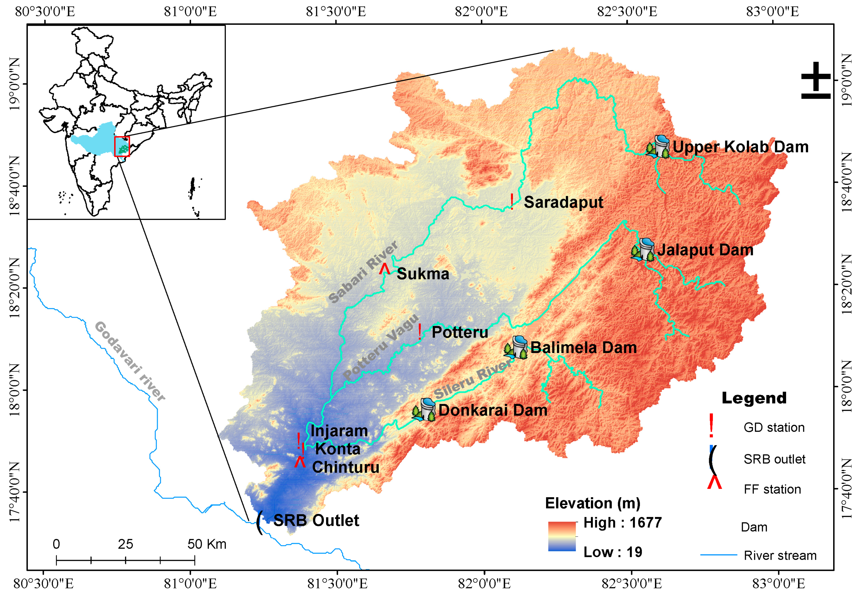
The Sabari River is one of the major tributaries of the Godavari River. It originates in the Eastern Ghats of Odisha state, where it is known as the Kolab River. The river confluences with the Godavari River near a village, Kunavaram, Telangana, India. The drainage area of the SRB is approximately 21,121 km² and extends between 81°5’23.147″E, 17°31’28.603″N and 83°2’43.912″E, 19°6′23.357″N (Figure 1). Elevation of the SRB ranges from 19 m to 1675 m, and most of the upstream of the basin is at or higher than 1000 m. The major land use and land cover (LULC) in the SRB is agriculture and forest (85%), followed by water bodies (10%) and built-up area (5%) [45]. Sandy clay loam, clay loam and clay are the three major types of soil, and C and D hydrologic soil groups are predominant in the SRB [46].

The SRB receives an average seasonal rainfall (June to September) of 1077 mm (calculated for 1966–2017). The SRB has four gauge-discharge (GD) stations and two-level flood forecasting (FF) stations. While GD stations record streamflow and gauge values, FF stations provide the flood warning issued as water level. Konta is the most downstream station among all the four GD stations, and it is in close proximity to the outlet of the basin. Therefore, Konta is treated as an outlet of the basin. The other three GD stations, Injaram, Potteru and Saradaput are the three stations in the interior of the basin. Average daily rainfall and average daily streamflow at Konta for the south-west monsoon period (June to September) are 8 mm/day and 944 m³/s, respectively, and these values are relatively high as compared to the annual averages (3.8 mm/day and 460 m³/s).

3. Data

Daily streamflow data at Konta, Injaram, Saradaput, and Potteru GD stations are available for the period of record 1966 to 2017, 1966 to 2006, 1997 to 2005 and 1970 to 2015, respectively. The streamflow data was obtained from the Krishna Godavari Board Organization (KGBO), CWC, India. Among all GD stations, Konta has the longest period of the record from 1966 to 2017, and consideration of the common period of the record for all stations decreased the length of available data, and consequently, the number of major flood events available for calibration were reduced. Therefore, streamflow data from Konta was considered to define the flood events for model calibration. However, data of all four GD stations was considered to define flood events for model validation.

Daily gridded rainfall data of 0.25° × 0.25° spatial resolution was obtained from the India Meteorological Department (IMD) [47]. The gridded data was used to extract the weighted average rainfall for each sub-basin from six configurations for all the flood events. Sub-basin specific rainfall amounts for the selected events were given as input to the Hydrologic Engineering Center-Hydrologic Modeling System (HEC-HMS) model. The Shuttle Radar Topography Mission (SRTM) based digital elevation model (DEM) of 30 m × 30 m [48] spatial resolution was used to extract the river streams and basin’s physical characteristics. Land use and land cover (LULC) data of 100 m spatial resolution for the years 1985, 1995, and 2005 is available for the Indian region [45] from which the values corresponding to the SRB were obtained. Soil data for the SRB of approximately 2.5 km spatial resolution were obtained from Harmonized World Soil Database Version 3.0 [46]. The LULC and soil data were used in obtaining the excess rainfall related parameters. Similar to rainfall, sub-basin specific LULC and soil data were extracted from the corresponding gridded data.

4. Methodology

4.1. Selection of Flood Events

An event is defined as when the daily streamflow is greater than the 90th percentile threshold at least for five consecutive time steps and continues until the streamflow is less than the given threshold for four consecutive time steps [49]. Note that the events defined by the algorithm were plotted, analyzed and then revised with respect to start and endpoints. The final set of 70 events consist of 21 single peak (SP), 13 double peak (DP) and 36 multiple peak (MP) events. The top five events of higher magnitude in each category were selected and used to calibrate the model.

Table 1. Flood aspects at Konta GD station, i.e., peak flows (Qp), flood duration (t), time to peak (Tp) and accumulated rainfall (Rsum) for the selected 15 events used in the model’s calibration. The letters in the event name, i.e., SP, DP and MP, correspond to single-, double- and multiple-peak, respectively.

Event	Peak Flows (Qp, m3/s)	Flood Duration (t, Days)	Time to Peak (Tp, Days)	Accumulated Rainfall (Rsum, mm)
1986SP	20,187	42	26	206.13
1966SP	14,416.3	22	15	546.67
1968SP	10,414.4	23	10	262.97
2015SP	7468	21	12	359.88
1972SP	6889.1	16	6	230.29
2005DP	8853.8	16	9	395.46
1969DP	8415.5	27	19	190.39
1966DP	7591.2	28	6	362.73
1988DP	6494	37	20	467.6
1975DP	6166.5	28	4	355.59
2006MP	12181.5	78	9	1698.99
1969MP	9787.7	37	15	429.76
2014MP	9768.3	41	16	446.64
1984MP	8037.1	52	21	660.95
1978MP	7991.9	58	37	692.35

details the characteristics of the events including peak flow, duration, time to peak and accumulated rainfall of the event. Three events, viz., 2003SP, 1997DP and 2004MP of duration 10, 15 and 30 days were selected for model validation. Event characteristics for three interior locations, i.e., Injaram, Saradaput, Potteru, along with the basin outlet Konta are mentioned in

Table 2. Similar to Table 1, but for three interior locations of the Sabari River Basin (SRB) along with the outlet, Konta.

GD Station	Peak Flows (Qp, m3/s)			Time to Peak (Tp, Days)			Accumulated Rainfall (Rsum, mm)
	2003SP	1997DP	2004MP	2003SP	1997DP	2004MP	2003SP	1997DP	2004MP
Konta	3355	1896	5804	5	10	11	127.67	114.41	338.62
Injaram	3763	1832	4269	4	10	11	127.94	114.48	338.52
Saradaput	3187	880	1380	4	3	28	146.86	143.26	382.44
Potteru	119	543	941	7	9	10	173.25	86.3	313.95

.

4.2. Model Setup

The HEC-HMS model is a physically-based, semi-distributed hydrological model developed by the U.S. Army Corps of Engineers [50]. The model can be run in lumped and semi-distributed modes at different time intervals ranging from minute to daily time steps, and parameters can be estimated in both event and continuous modes [51]. The HEC-HMS grouped key rainfall-runoff processes into four components and wrapped multiple methods as one method to model each of these components. In the present study, the HEC-HMS model was applied on a daily time scale in the event mode. The Soil Conservation Service-Curve Number (SCS-CN) method [52] was used to compute the excess rainfall. The Clark’s unit hydrograph (UH) method [53] was adopted to compute the direct runoff. An exponential recession model was employed to estimate baseflow, and the Muskingum method [54] was used for the channel flow routing.

In this study, the SRB was delineated according to the stream network with five different area thresholds. The resulting set of sub-basins represents the spatial resolution, and each spatial resolution was treated as a configuration in the modeling context as per the number of sub-basins. The model was run in the semi-distributed mode for these configurations. Moreover, the entire basin was considered as a single unit, and the model was run in the lumped mode for the configuration. Thus, a total of six configurations, i.e., a lumped model and five semi-distributed models were considered in this study. Basin delineation and calculation of physical characteristics of river and sub-basin such as length, width, area, basin lag and slope for all configurations were performed using the HEC-GeoHMS tool [55]. The above physical characteristics were used to estimate the initial values of parameters using empirical equations [50]. All six configurations were exported to the HEC-HMS model environment to perform the event-based rainfall-runoff modeling. The model calibration procedure is mentioned below.

4.3. Model Calibration

The model calibration consists of the following two components, i.e., (1) estimation of initial model parameter values using well-established empirical relationships, and (2) estimation of optimal values of model parameters using only the HEC-HMS model’s Neldar-Mead simplex algorithm and in combination with trial-and-error.

4.3.1. Model Initial Parameter Estimation

The set of parameters consist of initial abstractions (I_a), curve number (CN) and percentage of impervious area (imp%) of SCS-CN method, time of concentration (T_c) and storage coefficient (R) of Clark’s UH method, initial baseflow (Q₀), recession constant (k), and ratio to peak (R_p) of recession baseflow method, and travel time (K) for flood wave and dimensionless weight (X) of the Muskingum method. The percentage of impervious area was calculated from satellite maps. Therefore, this parameter was not included in the model calibration. The equations to estimate the initial values of parameters are shown in

Table 3. List of the HEC-HMS model parameters and empirical equations used to estimate the initial values of parameters along with range of the values used in the calibration.

Serial Number	Parameter	Equation/Initial Value	Calibration Range
1	Curve Number (CN)	$C{N}_{composite}=\frac{{\displaystyle \sum }{A}_{i}C{N}_i}{{\displaystyle \sum }{A}_i}$	30–100
2	Initial abstraction (Ia) in mm	$S=\frac{25400}{CN}-254; I_a=0.3S$	0–500
3	Percentage of impervious area (imp%) in percentage	$imp\%=\left(\frac{A_{Built-up}}{A}\right)$ × 100	not applicable
4	Time of concentration (Tc) in hr a	${\mathrm{T}}_{\mathrm{C}}=1.08\left(\frac{A^{0.09}{L}^{0.16}}{s^{0.12}}\right)$	0.1–500
5	Storage coefficient (R) in hr a	$\mathrm{R} =1.625\left(\frac{A^{0.0710}{L}^{0.118}}{s^{0.1085}}\right)$	0.1–150
6	Initial baseflow (Q0) in m3/s/km2	0.035	0.01–1
7	Recession constant (k) b	$Q_t=Q_0{\mathrm{k}}^t$	0.3–0.95 c
8	Ratio to peak (Rp)	0.1	0.1–1
9	Travel time (K) in hr	$\mathrm{K} =\frac{l}{V_W} ; V_W=\frac{1}{B}\frac{dQ}{dy}$	0.1–150
10	Weighting factor (X)	$\mathrm{X}=\frac{1}{2}\left(1-\frac{Q_0}{B{S}_0{V}_W\mathsf{\Delta }x}\right)$	0–0.5

^a [56], ^b [57], ^c [50]

. Additional information related to rainfall-runoff methods of the HEC-HMS model can be found in the Supplementary Material (Section SI1).

Where $C{N}_{composite}$ is the composite curve number, i is the index of sub-basins of uniform land use and soil type, $A_i$ is the area of i^th sub-basin, $C{N}_i$ is the curve number for i^th sub-basin, $S$ is the potential maximum retention that represents mainly the infiltration occurring after runoff has started, $A_{Built-up}$ is the built-up area of a basin or a sub-basin, $L$ is the longest flow path of a sub-basin, $s$ is the slope of the channel, $l$ is the channel length, $V_W$ is the wave celerity, $B$ is the top width of the water surface, $\frac{dQ}{dy}$ is the slope of the rating curve at a known cross-section, ${\mathrm{Q}}_0$ is the reference flow from the inflow hydrograph, an average flow, midway between the baseflow and peak flow, $Q_t$ is the baseflow at any time t, $S_0$ is the frictional slope, and $\mathsf{\Delta }x$ is the length of the reach.

4.3.2. Model Parameter Optimization

The parameters I_a, CN, T_c, R, Q₀, k and R_p were optimized simultaneously using the simplex algorithm for the lumped model. For the remaining five configurations, i.e., for five semi-distributed models, only I_a and CN were optimized using the simplex algorithm and the remaining seven parameters were estimated in the trial-and-error mode one-by-one in the following order, i.e., T_c, R, Q₀, k, R_p, K and X. The parameter R was calibrated first in case of either high volumetric error or no error in time to peak flow corresponding to optimal values of I_a and CN. The range of values for which parameters can be varied during its calibration suggested by the HEC-HMS user manual is mentioned in Table 3. Optimal parameter estimation in the trial-and-error mode was stopped when the Nash Sutcliffe Efficiency (NSE) of simulations was greater than or equivalent to 0.4. The chosen NSE threshold is subjective and can be modified.

The HEC-HMS’s optimization routine Nelder and Mead Simplex algorithm was chosen to minimize the objective function, Peak-Weighted RMSE (PWRMSE) [50]. The PWRMSE is a measure that implicitly compares magnitudes of flow peak, volume and time to peak between observed and simulated hydrographs. As it is seen from the equation (Table 4), the measure is a weighted sum of squared differences of simulated flows and corresponding observed flows. The weight of each ordinate is proportional to its observed streamflow magnitude.

Streamflow hydrographs that were derived based on initial values of parameters referred to as the reference scenario, whereas streamflow hydrographs that were derived based on optimal values of parameters treated as the calibration scenario. Streamflow from both reference and calibration scenarios were evaluated by calculating multiple verification metrics, i.e., the correlation coefficient (r), Nash-Sutcliffe Efficiency (NSE), Root Mean Square Error (RMSE), Mean Absolute Error (MAE) [58], Percentage Bias (PBIAS) [59], Percentage Error in Peak flows (PEP) [50] and Error in Time to Peak (ETP). Table 4 shows the mathematical formulae of the objective function and verification metrics.

Table 4. Mathematical formulae of the objective function and verification metrics used for the model calibration.

Metric	Equation	Range
Peak-Weighted Root Mean Square Error (PWRMSE) (m3/s)	$Z={\left\{\frac{1}{NQ}\left[{\displaystyle {\displaystyle \sum }_{i=1}^{NQ}}{\left(O_i-P_i\right)}^2\left(\frac{O_i+\overline{O}}{2\overline{O}}\right)\right]\right\}}^{1/2}$	0 to ∞
Correlation coefficient, r	$\frac{{{\displaystyle \sum }}_{i=1}^N\left(O_i-\overline{O}\right)\left(P_i-\overline{P}\right)}{{\left[{{\displaystyle \sum }}_{i=1}^N{\left(O_i-\overline{O}\right)}^2\right]}^{0.5}{\left[{{\displaystyle \sum }}_{i=1}^N{\left(P_i-\overline{P}\right)}^2\right]}^{0.5}}$	−1 to 1
Nash-Sutcliffe Efficiency, NSE	$1-\frac{{{\displaystyle \sum }}_{i=1}^N{(O_i-P_i)}^2}{{{\displaystyle \sum }}_{i=1}^N{\left(O_i-\overline{O}\right)}^2}$	−∞ to1
Root Mean Squared Error, RMSE (m3/s)	$\sqrt{\frac{{{\displaystyle \sum }}_{i=1}^N{(O_i-P_i)}^2}{N}}$	0 to ∞
Mean Absolute Error, MAE (m3/s)	$N^{-1}{\displaystyle {\displaystyle \sum }_{i=1}^N}|O_i-P_i|$	0 to ∞
Percent bias, PBIAS (%)	$\frac{{{\displaystyle \sum }}_{i=1}^N(O_i-P_i)}{{{\displaystyle \sum }}_{i=1}^N{O}_i}\times 100$	−∞ to ∞
Percentage Error in Peak, PEP (%)	$\left[\frac{(O_{Q_P}-P_{Q_P})}{O_{Q_P}}\right]\times 100$	−∞ to ∞
Error in Time to Peak, ETP (number of days)	$Dat{e}_{Q_{PP}}-Dat{e}_{Q_{PO}}$	−∞ to ∞

Table 4. Mathematical formulae of the objective function and verification metrics used for the model calibration.

Metric	Equation	Range
Peak-Weighted Root Mean Square Error (PWRMSE) (m3/s)	$Z={\left\{\frac{1}{NQ}\left[{\displaystyle {\displaystyle \sum }_{i=1}^{NQ}}{\left(O_i-P_i\right)}^2\left(\frac{O_i+\overline{O}}{2\overline{O}}\right)\right]\right\}}^{1/2}$	0 to ∞
Correlation coefficient, r	$\frac{{{\displaystyle \sum }}_{i=1}^N\left(O_i-\overline{O}\right)\left(P_i-\overline{P}\right)}{{\left[{{\displaystyle \sum }}_{i=1}^N{\left(O_i-\overline{O}\right)}^2\right]}^{0.5}{\left[{{\displaystyle \sum }}_{i=1}^N{\left(P_i-\overline{P}\right)}^2\right]}^{0.5}}$	−1 to 1
Nash-Sutcliffe Efficiency, NSE	$1-\frac{{{\displaystyle \sum }}_{i=1}^N{(O_i-P_i)}^2}{{{\displaystyle \sum }}_{i=1}^N{\left(O_i-\overline{O}\right)}^2}$	−∞ to1
Root Mean Squared Error, RMSE (m3/s)	$\sqrt{\frac{{{\displaystyle \sum }}_{i=1}^N{(O_i-P_i)}^2}{N}}$	0 to ∞
Mean Absolute Error, MAE (m3/s)	$N^{-1}{\displaystyle {\displaystyle \sum }_{i=1}^N}|O_i-P_i|$	0 to ∞
Percent bias, PBIAS (%)	$\frac{{{\displaystyle \sum }}_{i=1}^N(O_i-P_i)}{{{\displaystyle \sum }}_{i=1}^N{O}_i}\times 100$	−∞ to ∞
Percentage Error in Peak, PEP (%)	$\left[\frac{(O_{Q_P}-P_{Q_P})}{O_{Q_P}}\right]\times 100$	−∞ to ∞
Error in Time to Peak, ETP (number of days)	$Dat{e}_{Q_{PP}}-Dat{e}_{Q_{PO}}$	−∞ to ∞

Where Z is the objective function, $NQ$ is the number of hydrograph ordinates, N indicates the number of observations or the duration in days of the event; $O$ and $P$ are the observed and simulated values; $\overline{O}$ and $\overline{P}$ correspond to the average of observed and simulated values; $Q_{PP}$ is the peak flow of simulated hydrograph and $Q_{PO}$ is the peak flow of the observed hydrograph.

4.4. Model Validation

As part of the model validation, streamflow for the three flood events was estimated and then verified at all four selected locations, i.e., the basin’s outlet and three interior locations of the basin, i.e., Injaram, Saradaput and Potteru. The model parameter set consists of CN, I_a, T_c, R, k, Q₀, R_p, K and X, and calibration of the model for each event yields an optimal value for each parameter. Thereby, 15 events together result in a set of 15 values for each of the model parameters. In this way, first, an ensemble set of parameters was created, and then, a corresponding ensemble of streamflow was produced for the three selected events at all four selected locations. However, noting that the CN and I_a values as event specific as they depend on antecedent moisture conditions (AMC), the values of these parameters were not taken from calibration, consequently, the parameters were not part of the ensemble set of parameters. Similar to the calibration phase, the CN values were estimated for each event using rainfall five days prior to the event and LULC [60], and I_a was calculated as 30% of the potential maximum retention (S) (Table 1). The ensemble of streamflows was evaluated using the verification metrics shown in Table 4 as well as the Continuous Ranked Probability Score (CRPS), which is an ensemble verification metric [61]. The metrics in Table 4 are single-valued measures, and the ensemble mean of all ensemble members was used here. Thus, the model output in the validation mode was evaluated in both single-valued and ensemble modes.

5. Results and Discussions

5.1. The Six Configurations of Sabari River Basin

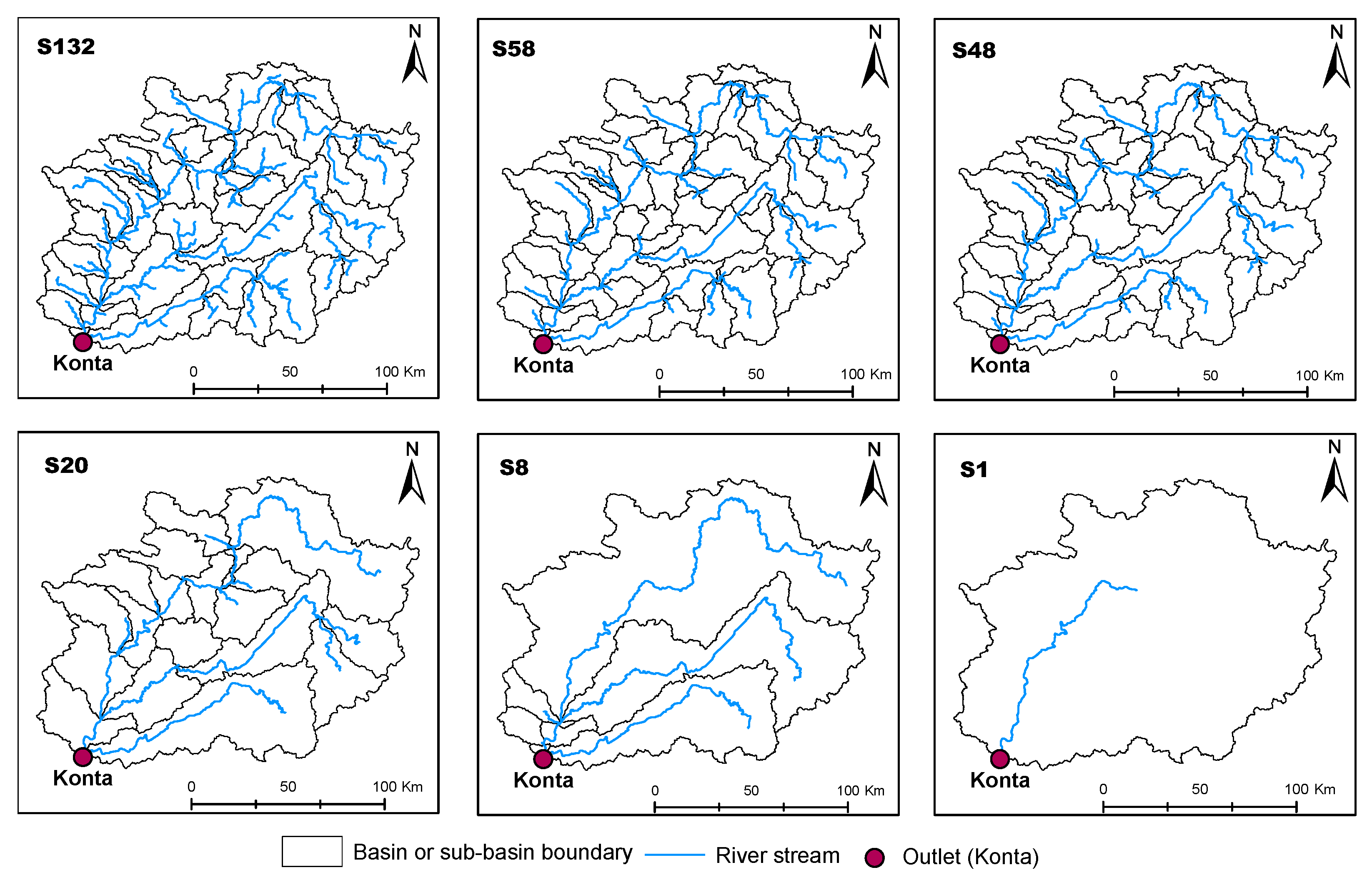
Figure 2 displays sub-basins that resulted from six configurations. The configuration that has no sub-basins resulted from treating the entire basin as a single unit and is named as S1. The configurations that were generated with five different area thresholds produced as small as eight to 132 sub-basins (

Table 5. Average values of topographical parameters of Sabari River Basin. The values for six configurations were calculated by taking the average value of all sub-basins of the corresponding configuration. Here, A_t is the threshold area used to delineate the configuration, A is the mean area of the basin, L is the mean longest flow path, and Lag is the basin lag.

Configuration	Threshold Area (At, km2)	Mean Area (A, km2)	Mean Longest Flows Path (L, Km)	Mean Basin Lag (Lag, h)
S1	Not applicable-	Not applicable	171.05	60.00
S8	300	2515	131.99	16.75
S20	450	1006	82.27	8.00
S48	225	419	49.77	5.36
S58	205	347	45.34	4.58
S132	90	152	29.00	3.31

). Accordingly, the basin configuration was named S8, S20, S48, S52 and S132. Sub-basins in all configurations except S8 were algorithm-based and automatic. The S8 was resulted from merging of a few sub-basins with a small stream order so that basins with only the highest stream order were retained. The logic behind the S8 is to perform the rainfall-runoff calculations by considering the tributaries that are directly joining the Sabari river. As the spatial resolution becomes finer, a few sub-basins are further divided into smaller sub-basins, and a few remained intact. Note that a sub-basin of S8 contains one or multiple reservoirs, whereas a sub-basin of a finer configuration typically contains only a part of the reservoir. Thus, basins with finer configuration require multiple sub-basins to encompass completely or a part of the reservoir.

Several topographical parameters, i.e., area, longest flow path, elevation, average channel slope, average basin slope and basin lag, were calculated for all the sub-basins for the six spatial resolutions. Table 5 displays basin/sub-basin average values of topographical parameters. As the spatial resolution became finer, the sub-basin average values of parameters were decreased. The values for the six configurations differed significantly suggesting basins of a different order. The relation between area and physical characteristics was found to be a power-law; thus, the characteristics exhibited scaling with respect to the basin or sub-basin area.

5.2. Results from the Model Calibration

As mentioned in Section 4.3.2, the set of seven parameters were optimized simultaneously for S1. For the remaining five configurations, the set of nine parameters were optimized. The two parameters, I_a and CN were optimized simultaneously, and the remaining seven parameters were optimized one-by-one through trial-and-error. The calibration was continued until the NSE of the simulations was greater than or equal to 0.4. It was observed that both baseflow and routing related parameters (k, Q₀, R_p, K and X) have less influence in improving the NSE of simulations, therefore these parameters were always assigned with their initial values. This leaves excess rainfall and direct runoff related parameters (CN, I_a, T_c and R) as active in terms of calibration; hence optimal values of these parameters were analyzed for six spatial resolutions with respect to 15 flood events and event characteristics. The following sub-sections detail how these optimized parameters vary in multiple aspects.

5.2.1. Spatial Resolution

The set of calibrated parameters was analyzed for 15 events for six spatial resolutions in the context of basin response as well as basin area. Figure 3 has four panels, and each panel corresponds to a parameter. Each panel has six boxplots, and each boxplot corresponds to a configuration. A filled circle in each boxplot correspond to a sub-basin’s parameter value for an event of a configuration. Thus, filled circles represent all values of a parameter for 15 events and all sub-basins of the configuration. Importantly, a boxplot with filled circles highlights whether values take only a certain portion of the range or vary continuously throughout the range, thus provides information on their distribution. Increased sample size (number of filled circles) was observed for finer resolution configurations because of an increase in the number of sub-basins.

A skewed and a horizontal band of values were observed for all the configurations and four parameters (I_a, CN, T_c, R). A skewed distribution implies a unique response of a sub-basin, where a long right or left tail of values was observed. Whereas the horizontal band of values suggests either a similar response of a sub-basin irrespective of the event or a similar response of all sub-basins to an event, hence the same set of values was observed. In this regard, the values of the parameters were analyzed with respect to the sub-basin area (Supplementary Materials Figure SI1–SI5) and an event. Although the sample size of the parameters for each configuration is different, the following was observed. The median of the values for parameters I_a, CN, T_c and R is high (low) for the S20 (S132, S48 and S1), S48 (S58 and S1), S1 (S58 and S8) and S1 (S132, S58, S4, S20 and S8) configurations, respectively. The results indicate the dominance of no single configuration across all parameters either for high or low values.

Noting that each parameter corresponds to a different physical process, the results suggest a different response of sub-basins of a configuration for each process and an association among parameters of a configuration. For example, relatively large I_a values of the S20 configuration indicate dry antecedent moisture conditions and are in accordance with the corresponding moderate CN values. Moreover, relatively low T_c values are in accordance with observed high R values for the S58 configuration. Other notable observations are decreased R values for configurations of finer spatial resolution (S8 to S132) and exponentially increasing R values with respect to the basin area, e.g., for S58 configuration (Figure SI6). The higher the R, the longer it takes for attenuation of peak flow and this was observed for larger basins. Thus, the results are consistent.

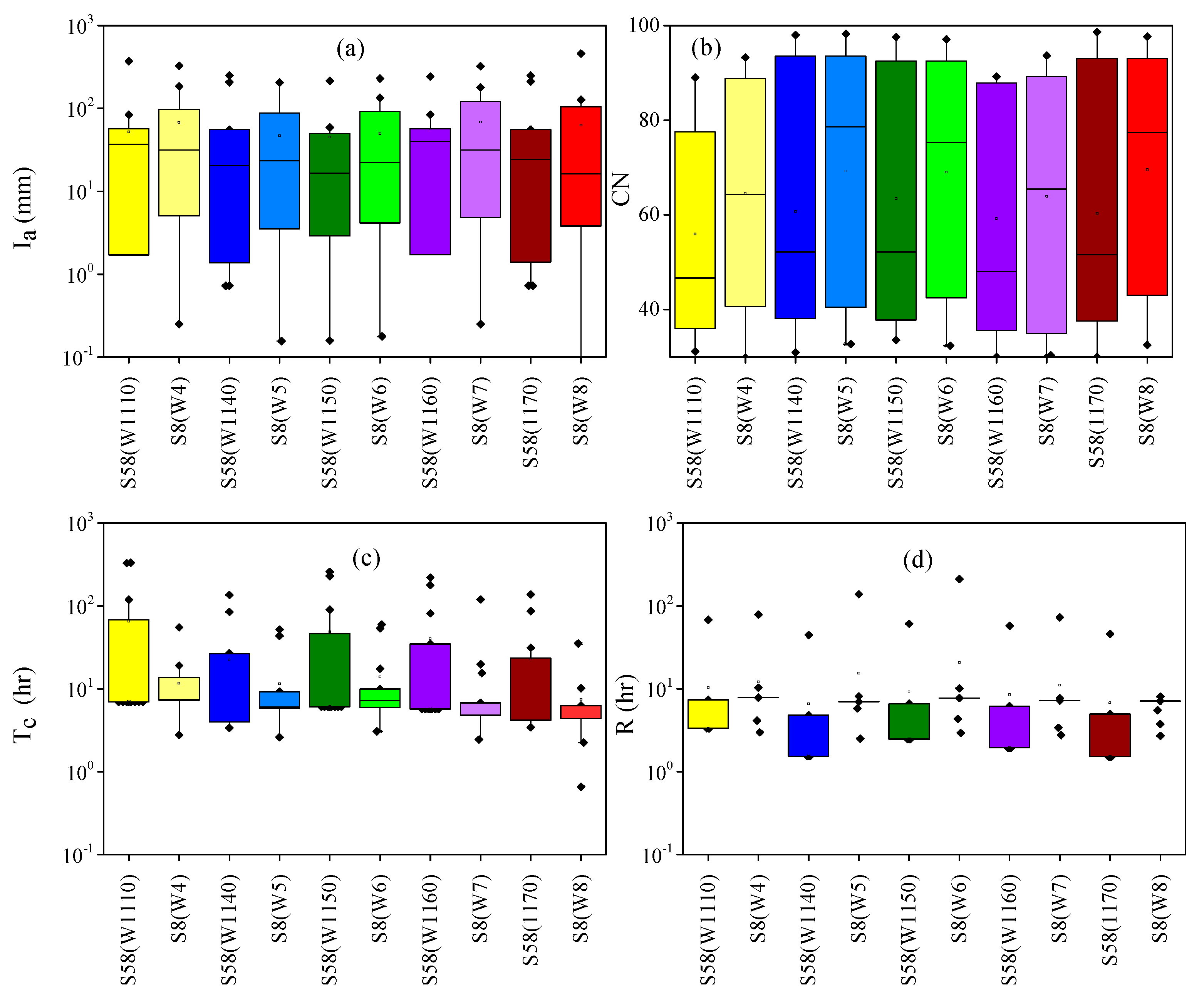
Apart from the above analysis, the values of parameters for sub-basins that are common in both S8 and S58 configurations were analyzed (Figure 4). A total of five sub-basins were chosen and were named differently in two different configurations. The common basins for both configurations were named in S58 (S8) as W1110 (W4), W1140 (W5), W1150 (W6), W1160 (W7) and W1170 (W8). The boxplot of values for the same basin of two configurations indicates that the parameters are not similar in their magnitude and distribution. The above implies that the response of a basin is different when it is modelled with a different configuration. However, this is not valid because the basin’s response will be the same irrespective of the configuration. All parameters, except I_a, exhibited an association with the sub-basin area (Supplementary Materials Figure SI1–SI5). However, a medium or large spread of parameter values implies a significantly different basin response and raises questions on the transferability of parameters for a basin for all events. In this regard, the values of the parameters were analyzed for each event separately.

5.2.2. Selected Flood Events

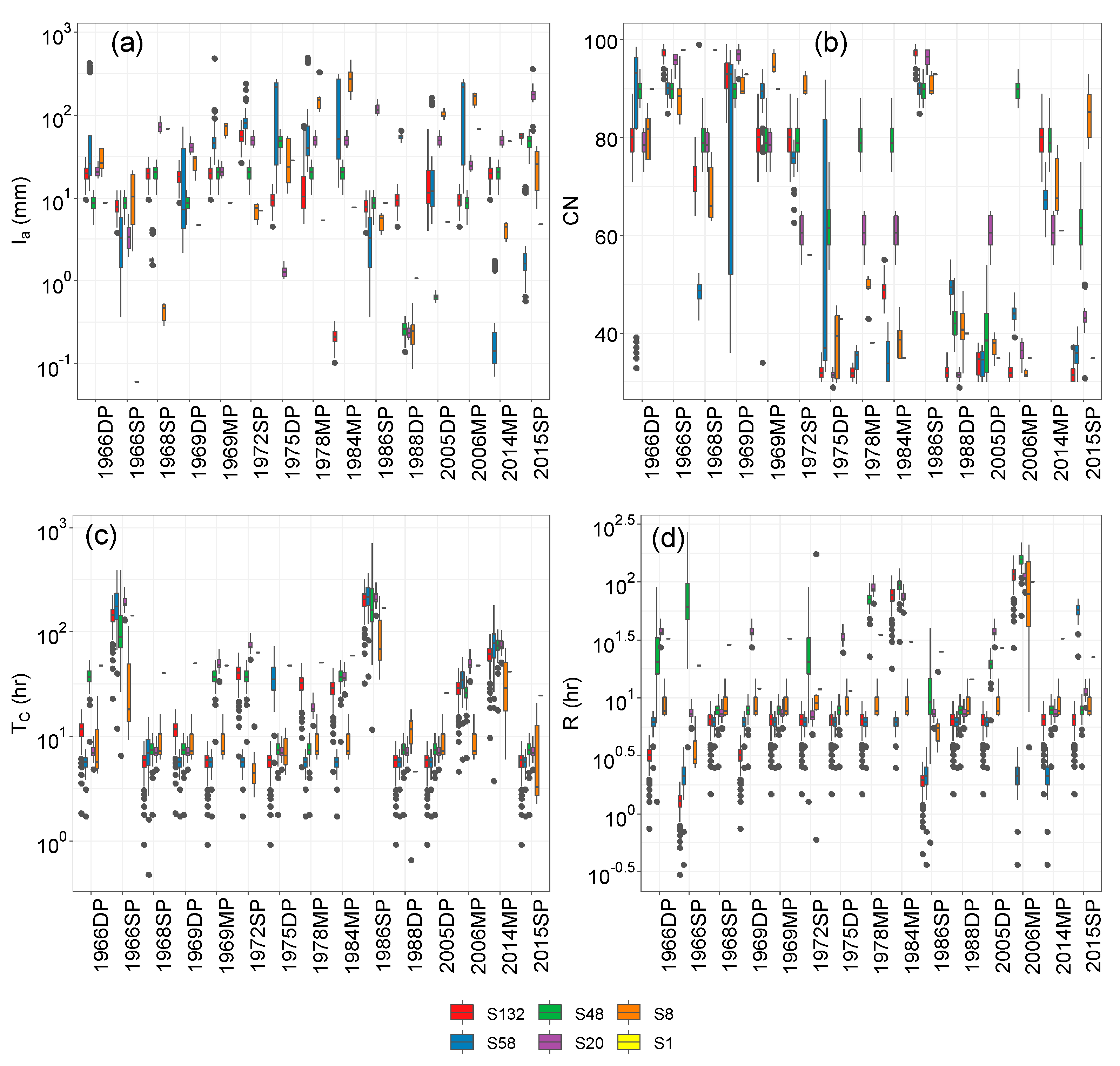
Figure 5 has four panels, and each panel corresponds to a parameter. Calibrated parameter values of all sub-basins of a configuration specific to an event are displayed in a boxplot. A set of six boxplots, of which each boxplot is in a different color and corresponds to a configuration, were developed for each event, and are arranged in chronological order of events. A filled circle in a boxplot corresponds to a value of the parameter for a sub-basin. Thus, the number of filled circles in each boxplot is equivalent to the number of sub-basins of the configuration. A notable observation among all plots is the pattern exhibited by the CN, i.e., high and low CN values for events of the early- and recent- part of the record. High CN values correspond to less infiltration, which may potentially result in higher runoff. However, it is a counter-intuitive observation to see high CN values in the early part of the record before any significant development in the basin. Apart from CN, no other parameters exhibited a pattern except that the range of values for a few parameters is high for certain events.

Except for I_a and CN values of S58 configuration, the boxplots broadly suggest no large variations in parameter values among sub-basins of the same configuration (indicated by boxplot of small size) and all configurations of an event (indicated by a set of boxplots corresponding to an event). However, the boxplots of values indicate a large event-to-event variability, particularly for I_a values (Figure 5a). Moreover, patterns with small variability in CN values (Figure 5b) and moderate to small variability in T_c and R values (Figure 5c,d) are mainly responsible for the boxplot of values to be different for six configurations were observed. Nevertheless, excluding 1966SP and 1986SP, no event with a combination of a parameter set with either high or low values was observed. In this regard, parameters were analyzed with respect to flood event characteristics.

5.2.3. Event Characteristics

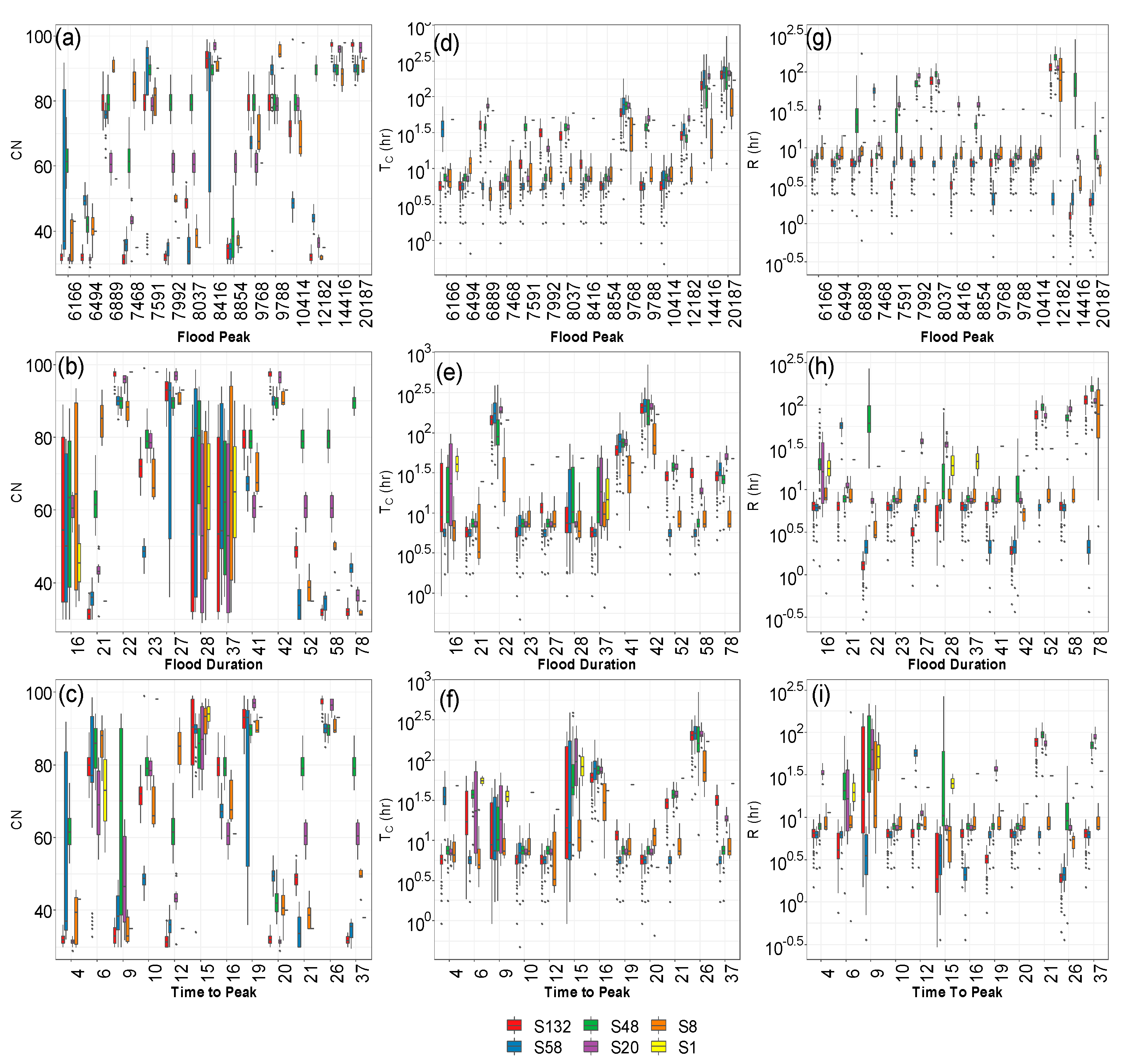
Four characteristics of a flood event, i.e., peak flow (Q_p), event duration (t) and time to peak (T_p), and accumulated rainfall (R_sum), corresponding to the event were considered as part of the analysis (see Table 1). While the time-to-peak values are uniformly distributed, flood duration values are relatively less right-skewed than the flood peak values (Figure 6). Rainfall amount increased with an increase in the flood duration of an event. With an event exclusion, two aspects, i.e., flood duration and flood peak exhibited a moderate linear association. However, flood magnitude exhibited no apparent association. As no clear pattern is observed among different aspects of flood events, parameters of all configurations were analyzed with event characteristics (Figure 7).

In Figure 7, each row corresponds to an event characteristic, and each column corresponds to a parameter. As parameter I_a was not exhibiting any specific pattern with any event characteristic, the corresponding association plot is not shown in Figure 7. Relatively high CN values were observed for high peak flow events and value greater than 70 were observed for approximately eight events for most of the configurations. High CN values with a small spread (i.e., small boxplot) were observed for the two highest peak flow events (Figure 7a). The large spread in CN values for three specific flood durations (16, 28 and 37 days) suggests that the CN values are different for flood events with the same flood duration (Table 1; Figure 7b). The difference in CN values reflects the different infiltration conditions, which can be attributed to different antecedent rainfall and soil moisture conditions of the events. Unlike for flood duration, the large spread in CN values for three different time to peak values (6, 9 and 15 days) was seen in all configurations and it indicates different responses from sub-basins of a configuration (Figure 7c).

Most T_c values for many configurations fall within a range of values from 3 to 10 h. High T_c values (~10 h) were observed for two flood events of high peak flow for all configurations (Figure 7d). Typically, high T_c values can be related to flood events of large magnitude for which most of the basin contributes as well as large flood events that result from high rainfall events in mid- and down-stream sub-basins. Thus, spatial variability of rainfall plays a key role in T_c values, and it is dominant for all configurations except S1. This also explains the relatively high T_c values of the S1 configuration. T_c values of the S1 were increased with respect to flood duration (Figure 7e), and it can be attributed to high rainfall amount ignoring spatial variability; typically, in these conditions, increased rainfall is associated with increased flood duration. Similar to CN values, the large spread in T_c values for the same flood duration and time to peak was observed and it is due to combining values from different flood events of the same flood duration or same time to peak (Table 1; Figure 7e,f).

Storage coefficient (R) values of S1 increased with peak flow magnitude; however, approximately similar values were observed for S8 (Figure 7g). Relatively, smaller R values were observed for S58 and S132, and they exhibited event-to-event variation only for a few events. The R values indicate the number of hours that a basin can temporarily store the excess rainfall, and it explains relatively small values for the basins of finer resolution as compared to the basins of coarser resolution. The three large sub-basins of S8 (see Figure 2) have one or more hydraulic structures which can store the excess rainfall during the event; therefore, similar R values were observed for S8. Similar to CN and T_c values, the R values for the flood events of the same flood duration or time to peak differ significantly (Table 1; Figure 7h,i). The two events with the same flood duration and time to peak resulted in a large spread (large boxplot) of R values. Note that there are also a few flood events for which R values are the same. Therefore, no large spread was observed, e.g., 1972SP, 2005DP,1988DP and 1969MP.

5.2.4. Performance Metrics

Model performance was analyzed by calculating various verification metrics using estimated and corresponding observed streamflow values for six configurations, for the 15 events. The verification metrics consist of r, NSE, RMSE, MAE, PBIAS, PEP and ETP, and were calculated separately for streamflow of reference and calibrated scenarios (

Table A1. Verification metrics for streamflow simulations of the reference scenario; verification metrics from left to right column are r, NSE, RMSE, MAE, PBIAS and PEP for six configurations, and each row corresponds to an event.

Event	Pearson Correlation Coefficient (r)						Nash-Sutcliffe Efficiencey (NSE)						Root Mean Square Error (RMSE)
	S132	S58	S48	S20	S8	S1	S132	S58	S48	S20	S8	S1	S132	S58	S48	S20	S8	S1
1986SP	0.47	0.48	0.52	0.41	0.58	0.63	0.15	0.17	0.23	0.04	0.31	0.37	5118.88	5080.12	4879.84	5455.93	4618.44	4411.23
1966SP	0.43	0.40	0.52	0.32	0.64	0.71	−0.07	−0.28	−0.04	−0.11	0.09	−0.01	4657.01	5111.15	4595.99	4764.48	4298.19	4534.46
1968SP	0.93	0.86	0.96	0.84	0.85	0.95	0.82	0.10	0.86	0.69	0.67	0.68	1068.81	2374.82	924.15	1395.14	1443.25	1419.53
2015SP	0.91	0.86	0.86	0.92	0.35	0.83	−1.05	−2.27	−0.79	−2.58	−0.42	−1.37	3019.58	3814.38	2822.60	3991.26	2518.43	3248.37
1972SP	0.92	0.93	0.96	0.74	0.97	0.98	−0.17	−0.66	0.11	−1.90	−0.20	0.54	2133.86	2539.65	1859.45	3355.05	2157.22	1336.20
2005DP	0.96	0.95	0.96	0.87	0.65	0.86	−2.03	−1.44	−1.15	−2.50	0.05	−0.51	3836.96	3442.04	3233.00	4122.93	2147.18	2712.62
1969DP	0.84	0.86	0.85	0.77	0.75	0.85	0.59	0.65	0.59	0.55	0.43	0.55	1100.69	1016.35	1092.58	1153.14	1291.11	1148.58
1966DP	0.91	0.91	0.92	0.88	0.91	0.94	0.81	0.81	0.82	0.68	0.77	0.84	734.79	735.25	717.34	944.85	810.78	680.04
1988DP	0.70	0.43	0.66	0.76	0.48	0.67	−0.03	0.14	0.03	−0.33	−0.71	−0.69	1322.45	1204.08	1283.42	1500.39	1698.36	1689.17
1975DP	0.91	0.89	0.90	0.80	0.84	0.89	−0.51	0.67	0.06	−2.73	−2.43	−1.08	1407.16	659.26	1112.53	2213.73	2124.83	1655.59
2006MP	0.63	0.63	0.67	0.51	0.74	0.79	−5.44	−4.92	−4.38	−6.71	−5.38	−2.55	6882.41	6599.83	6290.87	7531.05	6850.24	5113.00
1969MP	0.84	0.84	0.86	0.75	0.89	0.94	0.70	0.71	0.74	0.48	0.78	0.85	1326.04	1315.39	1241.21	1753.40	1124.58	928.52
2014MP	0.61	0.54	0.62	0.47	0.67	0.68	0.24	0.17	0.31	−0.12	0.38	0.42	1693.96	1774.77	1614.52	2054.33	1530.16	1485.55
1984MP	0.80	0.81	0.83	0.60	0.89	0.90	−1.12	−0.14	−0.99	−2.87	−1.67	−0.19	2332.54	1706.15	2256.04	3147.65	2614.85	1750.01
1978MP	0.82	0.82	0.82	0.76	0.75	0.81	−0.02	−0.19	0.09	−0.61	−0.28	0.24	1650.69	1777.40	1557.29	2069.51	1842.01	1425.39
Event	Mean Absolute Error (MAE)						Percent Bias (PBIAS)						Percent Error in Peak flows (PEP)
	S132	S58	S48	S20	S8	S1	S132	S58	S48	S20	S8	S1	S132	S58	S48	S20	S8	S1
1986SP	2600.49	2641.39	2528.20	2997.37	2386.76	2200.10	21.70	18.30	21.70	12.80	17.80	25.00	20.81	21.88	26.09	7.79	15.21	25.98
1966SP	2446.43	2792.20	2420.88	2461.57	2271.55	2478.39	180.10	414.20	208.40	141.90	183.20	246.10	54.87	81.60	60.68	43.86	52.58	72.32
1968SP	676.42	1372.62	641.37	864.60	742.86	699.81	19.10	162.50	17.80	16.30	33.00	43.40	23.45	72.92	24.04	14.74	21.70	50.19
2015SP	1770.01	2189.63	1699.86	2353.43	1715.73	2197.38	−52.00	−57.10	−50.10	−59.20	−27.40	−57.40	−99.99	−139.32	−93.64	−171.65	1.12	−89.48
1972SP	1203.88	1391.14	1042.55	1771.96	1071.33	935.79	−27.00	−33.90	−26.00	−35.90	−27.80	−26.10	−90.26	−107.95	−77.63	−113.78	−98.97	−41.52
2005DP	2441.92	2304.82	2245.28	2604.28	1506.53	1925.68	−47.30	−46.40	−45.70	−48.70	18.40	−42.40	−112.19	−94.80	−81.97	−135.32	−14.57	−54.44
1969DP	792.44	706.01	721.17	873.49	770.29	614.95	45.60	38.40	44.40	22.10	52.50	46.20	39.12	39.77	42.59	14.77	39.03	53.12
1966DP	555.86	541.65	557.56	696.48	629.57	557.51	−5.40	−9.50	−4.10	−16.80	−14.40	−12.90	28.16	25.79	31.83	13.65	12.74	24.22
1988DP	968.11	702.03	1002.39	1161.82	1236.25	1378.21	−37.50	15.00	−35.70	−43.50	−38.20	−48.00	20.72	55.56	29.33	−0.05	7.55	3.91
1975DP	994.18	514.45	866.49	1404.04	1274.32	1162.14	−45.40	−23.70	−41.60	−54.40	−52.70	−50.60	−57.91	4.97	−21.36	−95.10	−96.39	−46.71
2006MP	4115.94	4112.93	3840.79	4469.64	4531.14	3366.20	−58.90	−59.00	−57.70	−61.10	−62.90	−55.50	−253.12	−226.78	−227.83	−285.96	−268.98	−178.57
1969MP	830.42	810.39	768.79	1167.36	801.54	680.59	5.20	4.60	3.50	−4.00	3.90	9.50	−5.34	−1.87	−2.83	−15.65	−1.30	16.19
2014MP	1044.86	1020.87	962.64	1227.02	1033.01	871.91	6.10	45.90	11.10	−1.30	16.20	22.20	32.55	50.35	40.24	24.64	33.39	54.03
1984MP	1495.72	1150.07	1497.65	1854.15	1736.08	1267.21	−42.60	−33.10	−45.40	−48.80	−50.60	−43.40	−98.30	−65.11	−96.33	−148.68	−141.90	−59.07
1978MP	1232.74	1367.74	1193.07	1577.13	1327.79	1118.16	−27.60	−31.20	−28.00	−34.10	−30.80	−27.50	−41.92	−43.67	−36.65	−45.25	−38.96	−23.33
Event	Error in Time of Peak (ETP)
	S132	S58	S48	S20	S8	S1
1986SP	−3	−3	−3	−3	−2	−3
1966SP	−3	−3	−3	−3	−2	−2
1968SP	0	0	0	0	1	0
2015SP	1	1	1	0	2	1
1972SP	1	1	1	1	0	1
2005DP	1	1	1	0	1	1
1969DP	0	0	0	0	1	0
1966DP	0	−1	0	0	−1	0
1988DP	−10	11	11	−10	−9	−10
1975DP	0	0	0	0	1	0
2006MP	−1	−1	−1	−2	−1	−1
1969MP	0	0	0	−1	0	0
2014MP	−9	12	12	−9	13	−1
1984MP	−1	−1	−1	−1	0	0
1978MP	−1	0	0	0	1	0

and

Table A2. Verification metrics for streamflow simulations of the calibration scenario; verification metrics from left to right column are r, NSE, RMSE, MAE, PBIAS and PEP for six configurations, and each row corresponds to an event.

Event	Pearson Correlation Coefficient (r)						Nash-Sutcliffe Efficiencey (NSE)						Root Mean Square Error (RMSE)
	S132	S58	S48	S20	S8	S1	S132	S58	S48	S20	S8	S1	S132	S58	S48	S20	S8	S1
1986SP	0.94	0.92	0.93	0.94	0.95	0.96	0.70	0.72	0.65	0.70	0.73	0.77	3062.60	2957.57	3282.83	3051.76	2892.32	2682.37
1966SP	0.97	0.92	0.93	0.91	0.95	0.96	0.60	0.52	0.34	0.51	0.56	0.61	2849.74	3140.06	3655.97	3146.50	2988.00	2814.65
1968SP	0.92	0.95	0.95	0.85	0.90	0.99	0.85	0.84	0.90	0.72	0.81	0.98	963.38	987.00	795.42	1318.33	1092.39	378.02
2015SP	0.88	0.67	0.90	0.89	0.72	0.92	0.76	0.24	0.60	0.73	0.40	0.81	1041.06	1839.43	1330.76	1093.59	1635.54	917.79
1972SP	0.97	0.98	0.97	0.94	0.91	0.99	0.93	0.95	0.89	0.88	0.76	0.98	520.33	454.78	667.09	674.40	962.55	244.54
2005DP	0.95	0.95	0.97	0.93	0.64	0.95	0.79	0.84	0.84	0.64	0.16	0.89	1010.73	872.03	880.77	1319.41	2015.19	739.90
1969DP	0.87	0.85	0.82	0.81	0.77	0.85	0.73	0.69	0.64	0.56	0.56	0.71	885.44	955.43	1031.39	1130.24	1137.69	913.91
1966DP	0.93	0.93	0.95	0.90	0.91	0.94	0.84	0.86	0.84	0.77	0.79	0.84	662.51	632.66	662.63	808.09	761.07	680.04
1988DP	0.69	0.70	0.70	0.75	0.49	0.74	0.46	0.23	0.35	0.39	0.11	0.44	953.11	1143.66	1044.62	1013.31	1226.43	974.64
1975DP	0.90	0.93	0.90	0.90	0.77	0.93	0.80	0.85	0.68	0.69	0.53	0.84	518.64	440.94	646.79	638.50	782.40	455.91
2006MP	0.81	0.81	0.86	0.83	0.65	0.82	0.36	0.65	0.40	0.21	0.16	0.37	2164.97	1614.49	2102.33	2403.98	2490.76	2160.16
1969MP	0.89	0.90	0.89	0.93	0.94	0.94	0.76	0.78	0.76	0.85	0.85	0.85	1189.84	1145.96	1175.99	930.23	930.17	928.52
2014MP	0.72	0.66	0.70	0.71	0.72	0.67	0.44	0.39	0.44	0.49	0.46	0.41	1451.57	1522.37	1459.05	1391.97	1433.25	1487.57
1984MP	0.80	0.78	0.77	0.81	0.81	0.91	0.54	0.55	0.55	0.32	0.59	0.80	1091.34	1068.71	1074.01	1320.20	1022.82	708.96
1978MP	0.88	0.88	0.85	0.86	0.83	0.87	0.74	0.72	0.55	0.58	0.54	0.71	837.01	863.13	1089.93	1053.55	1109.89	874.70
Event	Mean Absolute Error (MAE)						Percent Bias (PBIAS)						Percent Error in Peak flows (PEP)
	S132	S58	S48	S20	S8	S1	S132	S58	S48	S20	S8	S1	S132	S58	S48	S20	S8	S1
1986SP	1886.34	2046.45	1819.89	1920.99	1715.78	1456.52	13.90	2.10	23.40	9.70	26.80	21.70	48.48	46.63	48.95	48.22	44.06	40.58
1966SP	1487.92	1757.26	2056.98	1740.25	1586.15	1559.57	60.80	59.60	109.30	56.70	80.20	61.70	53.10	57.21	66.67	59.21	52.17	51.64
1968SP	619.97	670.11	593.46	800.60	674.69	290.69	−2.10	4.80	−7.50	8.60	−2.00	−2.70	1.61	24.37	−3.91	5.09	−1.08	4.51
2015SP	564.42	1294.91	866.35	664.67	1198.14	541.53	12.00	−26.40	−23.30	−4.60	−25.00	−10.00	−3.57	0.40	−34.15	−19.30	−7.51	−15.59
1972SP	388.69	352.49	395.90	470.29	837.10	193.61	2.60	12.00	−9.20	2.90	−18.70	−1.60	−13.40	2.11	−13.42	−1.61	0.69	−0.48
2005DP	693.15	612.89	647.84	1020.47	1364.94	578.27	7.20	2.30	−7.70	−24.70	35.20	−1.40	−18.23	−13.09	−14.61	−10.79	2.49	0.18
1969DP	679.04	719.97	767.13	705.99	660.10	622.53	13.70	19.80	18.20	6.70	19.50	−7.50	23.40	33.80	19.14	−1.03	19.12	22.69
1966DP	537.11	470.71	524.54	616.25	595.84	557.51	−5.50	−6.00	−14.00	−13.90	−9.90	−12.90	23.43	23.70	22.10	16.97	19.33	24.22
1988DP	591.06	822.09	721.19	741.52	763.95	696.83	−6.90	−28.30	−23.90	−24.00	−14.40	−20.30	48.42	30.46	39.02	27.40	39.06	38.97
1975DP	437.67	344.87	482.85	453.83	449.04	384.60	−7.60	−8.50	−26.00	−22.50	−6.40	−10.40	12.59	15.61	17.68	3.23	7.49	10.36
2006MP	1691.45	930.67	1675.45	1881.46	1992.84	1589.23	−35.80	17.10	−38.20	−41.40	−32.30	−34.70	5.68	5.12	2.24	−4.97	−2.80	−0.39
1969MP	739.22	706.99	747.52	604.60	711.16	680.59	15.90	16.20	17.00	5.50	18.40	9.50	−0.22	1.29	3.07	−2.66	−1.16	16.19
2014MP	906.52	995.75	906.11	918.70	965.59	868.78	−8.60	−11.50	−4.90	7.60	−2.30	22.30	19.67	34.12	27.85	44.69	29.08	54.10
1984MP	869.64	687.76	842.65	1086.23	703.69	506.11	−23.80	2.80	−17.10	−33.90	9.60	−10.50	8.60	−2.83	22.98	−7.44	−10.92	−4.56
1978MP	518.37	600.08	852.98	770.13	736.47	611.64	12.70	8.80	−21.00	−19.30	15.20	12.00	1.76	−2.49	1.44	6.15	−0.98	7.66
Event	Error in Time of Peak (ETP)
	S132	S58	S48	S20	S8	S1
1986SP	0	0	−1	0	−1	−1
1966SP	−1	0	−1	0	−2	−1
1968SP	0	0	0	0	1	0
2015SP	1	1	0	0	1	1
1972SP	0	0	0	0	0	−1
2005DP	0	0	1	0	1	0
1969DP	0	0	0	0	1	0
1966DP	0	0	0	0	0	0
1988DP	1	1	11	−10	−9	−10
1975DP	0	0	0	0	1	0
2006MP	0	−1	0	0	45	0
1969MP	0	0	0	0	0	0
2014MP	8	7	8	8	7	−1
1984MP	0	−1	0	0	0	0
1978MP	0	0	0	0	1	0

). As seen in the table, each of these scenarios has 90 values for each verification metric and result from a combination of six configurations and 15 events.

Positive correlation coefficient (r) values for both scenarios were observed. For the calibration scenarios, approximately 92% of the values are greater than 0.7 and 50% of the values are greater than 0.9. High values of r, ~ 0.85 or greater values were observed for at least one of the six configurations when 1988DP and 2014MP are excluded. However, the r values for the reference scenario suggest its poor performance, yet 33% of values are greater than 0.9 and nine of 15 events exhibited a value of ~ 0.85 at least for one of the configurations. In terms of NSE, approximately 85% of the values were greater than 0.4 for the calibration scenario. However, both positive and negative values were observed for the reference scenario, i.e., 50% of the NSE values are smaller than zero, and 20% of the values are greater than zero and less than 0.4. For the calibration scenario, the highest NSE values were greater than 0.4 for at least one of the six configurations for all the events. Whereas, for the reference scenario, the highest values of greater than 0.4 were observed only for seven of the 15 events. These suggest the better performance of the calibration scenario. While the linear association among estimated and corresponding observed streamflow and performance of estimated streamflow with respect to climatology are essential, the difference in streamflow magnitude should not be large. Therefore, metrics based on error terms were estimated.

The error term corresponds to a flow magnitude, and it is challenging to set a threshold to define the best or acceptable value. In this regard, first, the configuration with the lowest error was identified. Second, the score “1” was assigned for configurations with error values under 25% of the lowest error; otherwise “0” was assigned. Thus, if the error is within 25% of the lowest error for all configurations, then all configurations get a score of “1” and are accepted as equally performing. Finally, the above criterion was repeated for all 15 events and configurations. A model score can range from 0 to 15, and a high score indicates a relatively better performing configuration. The scheme was extended for both r and NSE metrics, but configurations with the metric values within 10% of the best metric were considered. Similarly, the model scores were calculated for error in time to peak (ETP), and configurations with non-zero values were penalized with a score of “0”. The model scores were tabulated for all configurations of both reference and calibration scenarios, and the label of a column without the asterisk (*) corresponds to the reference scenario (

Table 6. Model scores were calculated for six configurations of both reference and calibration scenarios. A model score can range from 0 to 15, and a high score indicates a relatively better performing configuration. The label of a column without and with asterisk (*) corresponds to streamflow simulations of reference and calibration scenarios, respectively.

Verification Metric	S132	S132 *	S58	S58 *	S48	S48 *	S20	S20 *	S8	S8 *	S1	S1 *
Correlation coefficient, r	9	14	7	13	10	14	3	13	6	8	11	15
Nash-Sutcliff Efficiency, NSE	5	10	4	8	6	11	2	11	3	5	7	14
Root Mean Square Error, RMSE	3	9	2	11	3	6	0	6	2	5	3	14
Mean Absolute Error, MAE	2	9	4	9	3	7	0	5	1	5	4	14
Percentage of Bias, PBIAS	0	5	0	6	2	0	2	4	1	3	0	4
Percentage Error in Peak, PEP	0	4	0	5	0	1	4	6	2	5	0	5
Error in Time of Peak, ETP	5	11	5	10	6	10	7	13	3	4	7	9

).

Among all configurations of calibrated scenario, S1 stands out with very high model score values for four verification metrics (r, NSE, RMSE and MAE) followed by S132. Except for S8, all configurations exhibited similar scores for r and NSE. Whereas S1, S132 and S58 exhibited slightly higher values than S20 and S48 configurations in the case of RMSE and MAE. For PBIAS and PEP, all configurations exhibited relatively smaller model score, and among them, S132 and S58 have slightly higher values followed by S1. Low model score indicates no consensus on the best configuration, i.e., a few configurations performed better for certain events. The model score values for ETP suggest the relatively better performance of S20, S132, S58 and S48 compared to S1 and S8. When the threshold values of 25% and 10% were modified to 15% and 5%, respectively, no significant changes in the model scores were observed.

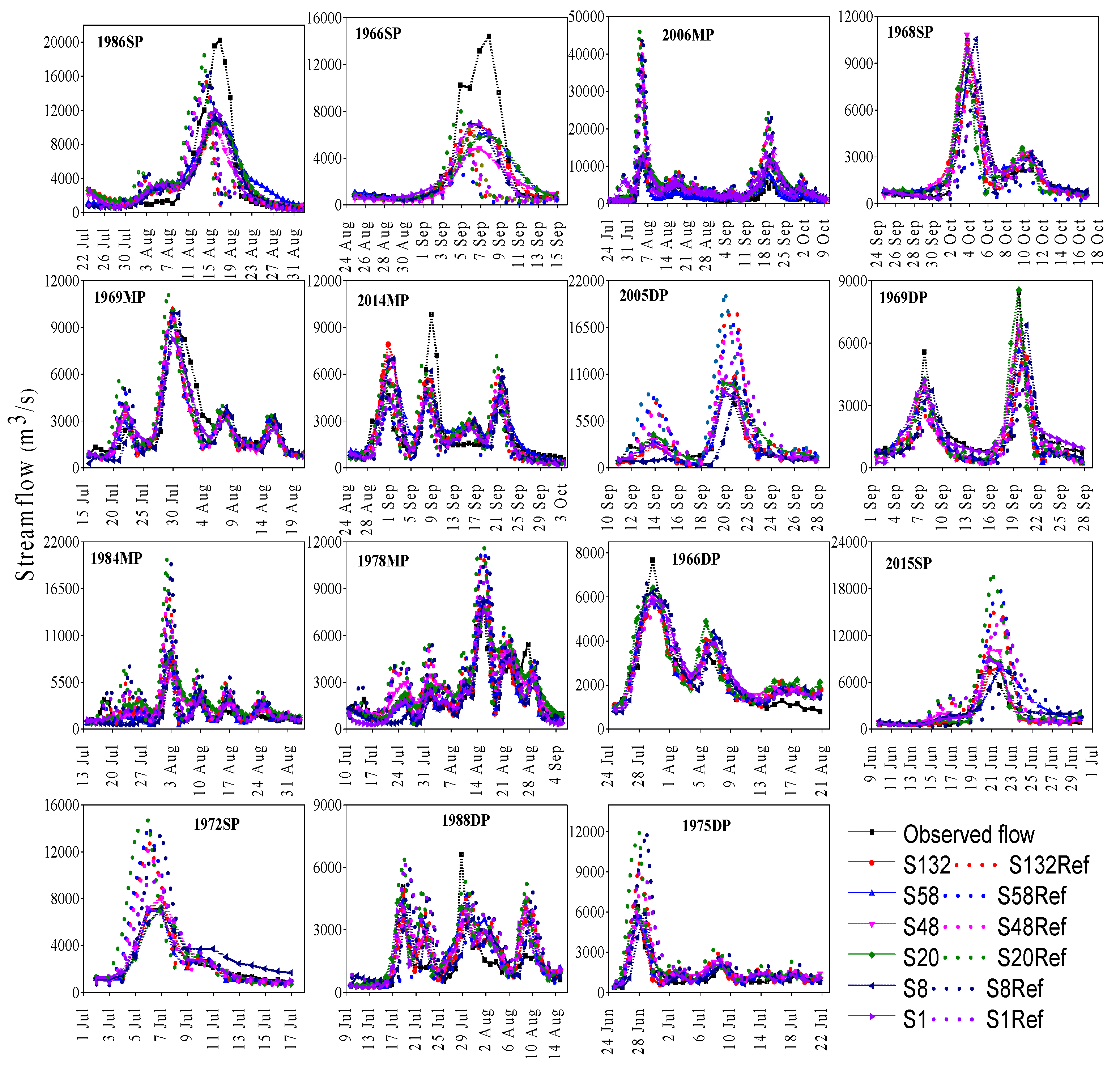
In addition to verification metrics, streamflow hydrographs were developed and used in the qualitative assessment of streamflow simulations. Figure 8 shows hydrographs of observed and estimated streamflow of reference and calibrated scenarios for six configurations, for 15 events. The plots are arranged in descending order based on magnitude of observed peak flow. Each plot has 13 hydrographs, of which one corresponds to observed streamflow, and two sets each with six hydrographs correspond to streamflow of reference and calibration scenarios.

Hydrographs of all events suggest that estimated streamflow from all configurations are realistic and exhibit day-to-day variations like observed streamflow. However, the plots also highlighted underestimated peak flow and volume for the two highest flood events, i.e., 1986SP and1966SP, and for a multi-peak flood event, i.e., 2014MP, for all six configurations, for both the scenarios. The large error for the two highest flood events indicates the model’s inability to simulate excess rainfall and its translation into direct runoff. For 1986SP, underestimated streamflow is attributed the backwater effect in the Sabari river due to the high streamflow in the Godavari river (main tributary). The backwater effect increased the streamflow at the Konta GD station, but it is not accounted for by the HEC-HMS’s regular direct runoff related calculations. Therefore, underestimated streamflow was produced. For the 1966SP, dry AMC resulted in incorrect CN values, which in combination with other parameters produced underestimated streamflow. The time to peak (T_p) was advanced by a day for S1, S8 and S48 (Table A1). Streamflow of the reference scenario was underestimated for six events, overestimated for another six events, and showed less bias for three events. In a similar proportion, time to peak was either advanced or delayed; however, no association was observed with either under-or over-estimated streamflow. Whereas streamflow of the calibration scenario was relatively better, i.e., exhibited less bias and correctly estimated time to peak, which was reflected in the model score as well. For the two events (1988DP and 2014MP), the time to peak was largely advanced or delayed for most of the configurations. The same was observed for 2006MP for the S8. The error can be attributed to the presence of two or more peaks of the same magnitude at longer days apart and overestimated peak flows for other than the actual peak. However, there are other events of two or more peaks for which most of the configurations have zero error in time to peak e.g., 1966DP, 1975DP and 1984MP.

5.3. Results from the Model Validation

The model calibration results suggested a better performance of S1 followed by S132. Given that S1 estimates streamflow only at the basin’s outlet and S132 estimates streamflow at both basins’ outlet and interior locations, S132 was considered for the model validation. The HEC-HMS model was run for three events at four locations (Konta, Injaram, Saradaput and Potteru) using the ensemble of parameter values that were obtained during the calibration. The parameter set consists of nine parameters, of which a total of five parameters from baseflow (Q₀, k and R_p) and routing (K and X) methods exhibited no significant variation irrespective of an event. Therefore, the same value of the parameter was used in the validation, i.e., no ensemble of values for these parameters. In addition, the excess rainfall method parameters are events specific, therefore, the parameters are not part of the ensemble set of parameter values. Thus, it results in an ensemble set of parameter values for direct runoff method, i.e., T_c and R.

The excess rainfall method parameters, i.e., I_a and CN, vary with each event, therefore the parameters were estimated separately for three events. The Clark’s UH parameters (T_c and R) of all events excluding two extreme events, i.e., 1966SP and 1986SP, were used. Thus, it potentially yields 13 sets of T_c and R. However, values for a set of events are the same. In this regard, T_c and R values of events, 1968SP, 2015SP, 2005DP, 1988DP, 1975DP and 1969MP were grouped as set 1, and events 1969DP and 1966DP were grouped as set 2. The values for the remaining five events (1972SP, 2006MP, 2014MP, 1984MP and 1978MP) are different and treated as a separate ensemble member. Thus, a total of seven sets of parameters were created.

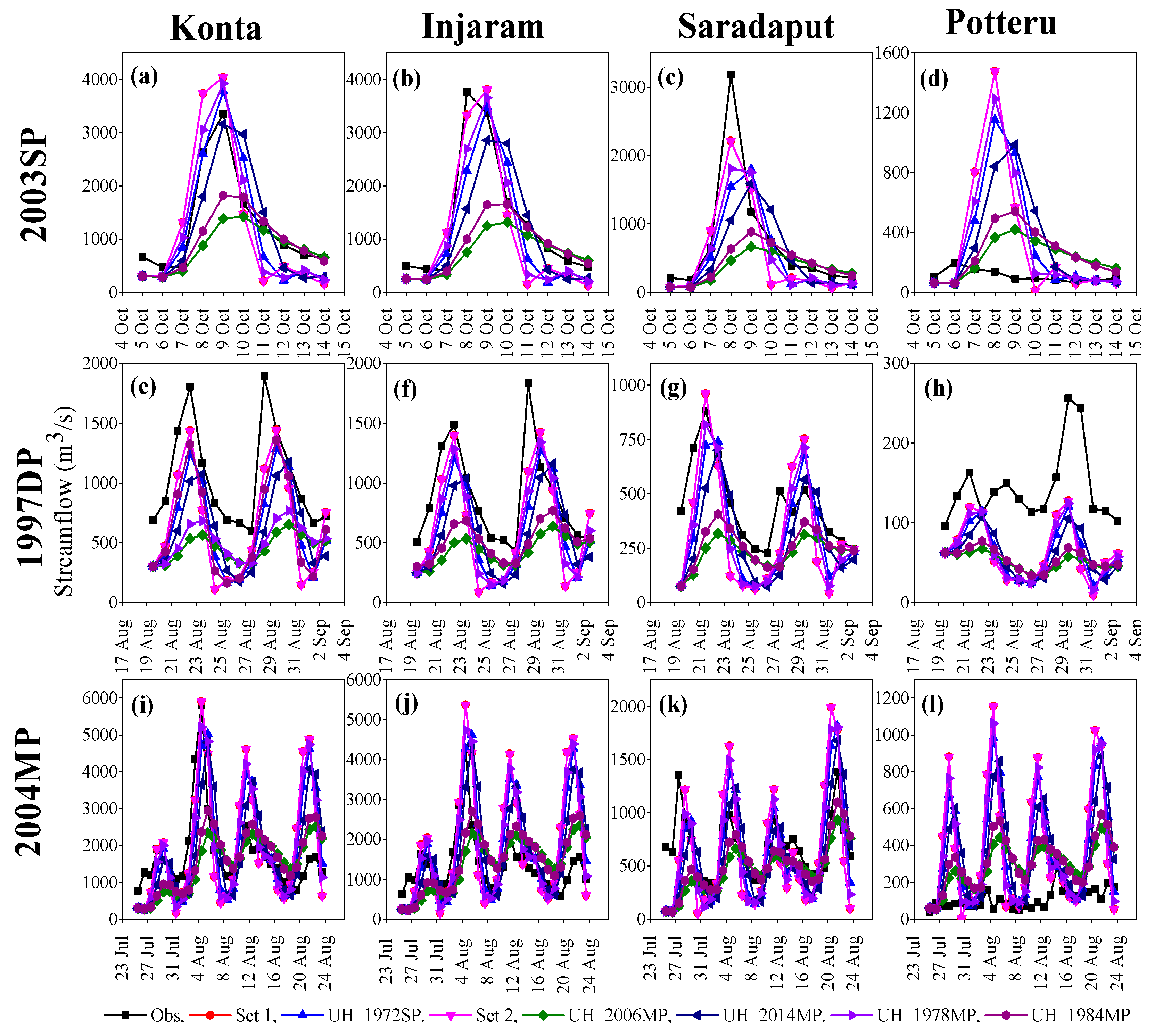
The ensemble of seven sets of parameters was used to generate an ensemble of streamflow for four locations, for three events (Figure 9). Both single-valued and mean continuous ranked probability score (CRPS) [61] were calculated using ensemble median and all ensemble members, respectively (

Table 7. Deterministic and ensemble verification metrics for three events at four locations.

Metric	2003SP				1997DP				2004MP
	Konta	Injaram	Saradaput	Potteru	Konta	Injaram	Saradaput	Potteru	Konta	Injaram	Saradaput	Potteru
r	0.96	0.90	0.83	0.14	0.82	0.73	0.72	0.48	0.57	0.63	0.66	0.15
NSE	0.88	0.70	0.51	−75.60	−0.55	−0.09	−0.23	−3.11	0.06	−0.32	−0.12	−35.85
RMSE	325.67	649.59	611.61	341.87	519.08	419.64	204.98	92.96	994.55	845.49	291.41	321.32
MAE	316.70	436.25	287.02	226.98	456.48	320.48	160.92	83.73	756.28	653.52	202.41	240.86
PBIAS	−14.00	−25.30	−34.00	175.00	−44.20	−36.40	−34.90	−58.50	2.70	21.20	−15.50	221.60
PEP	−10.06	−26.04	−57.12	376.48	−43.41	−42.19	−31.70	−60.61	−29.88	−12.35	9.95	184.16
ETP	0	1	1	2	1	1	0	0	1	1	0	−10
CRPS	235.77	303.96	246.52	163.13	368.51	260.41	132.53	77.28	585.31	507.37	170.86	185.90

). The mean CRPS considers all members of an ensemble forecast, and it reduces to the mean absolute error (MAE) of the single-valued forecasts. Thus, both mean CRPS and MAE can be compared. Performance of estimated streamflow varied with each event; however, relatively better performance was observed for 2003SP in terms of linear association and NSE (Table 7). The mean CRPS and MAE are of approximate values for most of the locations and events. Estimated streamflow at the Konta has exhibited relatively better performance, and it is intuitive as the HEC-HMS model calibrated with Konta streamflow.

In addition to the verification metrics, hydrographs for an ensemble of estimated streamflow were developed (Figure 9). Each ensemble member and all members together showed realistic estimated streamflows. The estimated streamflow exhibited day-to-day variability and produced single-, double and multiple peaks encompassing of observed streamflow for three events for all locations excluding Potteru. Note that the estimated streamflow corresponds to set 1 and set 2 were of the same values; therefore, they are not distinguished in the plot. The estimated ensemble of streamflows exhibited poor performance at the Potteru for events 2003SP and 2004MP; however, they appeared realistic for the event 1997DP with a systematic bias. The poor model performance at the Potteru for events 2003SP and 2004MP could be attributed to the controlled streamflows from upstream at the Jalaput reservoir, which has been operational since 2000. While no systematic pattern was seen for events for the remaining three locations, a few verification metrics suggest good performance with error metrics emphasizing post-processing of streamflows [62,63,64,65].

As the need for the basin-wide real-time forecast is imminent, reliable and accurate runoff estimates at customized locations of a basin including ungauged basins are necessary. The estimation of streamflow for the interior part of a basin requires a scientific understanding of hydrologic processes with respect to resolution and integration of information in the modeling context so that a robust forecast system can be developed. Insights gained from the analysis of parameter values and model performance with respect to sub-basin area, model spatial resolution and events assist in developing the system. The results suggest that the runoff estimates are chiefly driven by excess rainfall and direct runoff components. Equal performance of all configurations in Percentage Error in Peak (PEP, see Table A1 and Table A2) agree with [66], who observed smaller differences in the model performance metrics with an increase in spatial resolution for two flood events. However, no consensus was observed among configurations with respect to other verification metrics, and it requires further analysis.

As part of the future work to develop an operational real-time flood forecast system, the following needs to be considered. Sub-basin specific rainfall amounts with respect to events highlight the influence of spatial variability of rainfall. However, it warrants a detailed analysis (e.g., [36,37,51]). Channel routing is an essential component of modeling, and apparently, the Muskingum method did not exhibit any significant role. In this regard, other methods of channel routing need to be explored. In addition, a detailed analysis of rainfall-runoff modeling with finer and coarser resolutions to understand the anthropogenic effects (e.g., land-use change and the role of reservoirs) and integration of hydrologic information as per its availability, including for a short period of the record, is much needed.

6. Conclusions

The Sabari River Basin was delineated into six configurations, and event-based rainfall-runoff modeling was carried out using the HEC-HMS model. The model calibration and validation were performed for 15 and three flood events of single, double and multiple peaks. The calibrated parameters were analyzed with respect to spatial resolution (sub-basin area), flood events and event characteristics, and then performance metrics were calculated for the reference and the calibration scenarios. It was observed that the parameters vary among the sub-basins and all configurations for a given event. Values of the parameters suggest the key role of initial abstractions (I_a), curve number (CN), unit hydrograph related parameters, and less influence of baseflow and channel routing parameters. While I_a and CN varied event-to-event without any pattern, T_c and R exhibited similar values for most of the events for finer resolution configurations. Being unit hydrograph parameters, T_c and R represent the basin’s geomorphological characteristics. Therefore, approximate T_c and R values for most of the events are agreeable. The performance metrics highlight the better performance of S1 and S132 during the calibration. The hydrographs suggest realistic estimates of streamflow for most of the configurations and events. Noting that S1 estimates streamflow only at the basin outlet, S132 was used to estimate streamflow at four locations as part of the validation.

S132 was implemented with a set of seven unique values of calibrated parameters and produced an ensemble of streamflow for three events at four locations. Three of the four locations are interior locations of the basin; thus, the model validation mimics basin-wide streamflow estimates. While performance metrics for a few configurations suggested an agreeable performance, the estimated streamflow was not of similar accuracy as in calibration because of input forecast uncertainties [36,67,68]. As in calibration, streamflow hydrographs suggested realistic flows. However, streamflow estimation may be improved with post-processing including simple techniques for bias correction. Thus, this study shows the estimation of an ensemble of streamflows that can be further enhanced at the basin′s interior locations at multiple spatial resolutions. In addition, these types of studies need to be extended in the context of other aspects of modeling, for example, input—including rainfall and model structure—related uncertainties. To address the above limitations, a systematic analysis of rainfall-runoff modeling using other well-established hydrologic models and techniques is necessary, and this study can be treated as one of the steps in this direction.

References

- Beven, K. How to make advances in hydrological modelling. Hydrol. Res. 2019, 50, 1481–1494. [Google Scholar] [CrossRef] [Green Version]
- Singh, V.P. Hydrologic modeling: Progress and future directions. Geosci. Lett. 2018, 5, 1–18. [Google Scholar] [CrossRef]
- Sivakumar, B.; Singh, V.P. Hydrologic system complexity and nonlinear dynamic concepts for a catchment classification framework. Hydrol. Earth Syst. Sci. 2012, 16, 4119–4131. [Google Scholar] [CrossRef] [Green Version]
- Clark, M.P.; Schaefli, B.; Schymanski, S.J.; Samaniego, L.; Luce, C.H.; Jackson, B.M.; Freer, J.E.; Arnold, J.R.; Moore, R.D.; Istanbulluoglu, E.; et al. Improving the theoretical underpinnings of process-based hydrologic models. Water Resour. Res. 2016, 52, 2350–2365. [Google Scholar] [CrossRef] [Green Version]
- Hey, T.; Tansley, S.; Tolle, K. The Fourth Paradigm—Data-IntensIve ScIentIfIc Discover; Microsoft Research: Redmond, WA, USA, 2009. [Google Scholar]
- Peters-Lidard, C.D.; Clark, M.; Samaniego, L.; Verhoest, N.E.C.; Van Emmerik, T.; Uijlenhoet, R.; Achieng, K.; Franz, T.E.; Woods, R. Scaling, similarity, and the fourth paradigm for hydrology. Hydrol. Earth Syst. Sci. 2017, 21, 3701–3713. [Google Scholar] [CrossRef] [Green Version]
- Sivapalan, M.; Takeuchi, K.; Franks, S.W.; Gupta, V.K.; Karambiri, H.; Lakshmi, V.; Liang, X.; McDonnell, J.J.; Mendiondo, E.M.; O’Connell, P.E.; et al. IAHS Decade on Predictions in Ungauged Basins (PUB), 2003-2012: Shaping an exciting future for the hydrological sciences. Hydrol. Sci. J. 2003, 48, 857–880. [Google Scholar] [CrossRef] [Green Version]
- Borah, D.K. Hydrologic procedures of storm event watershed models: A comprehensive review and comparison. Hydrol. Process. 2011, 25, 3472–3489. [Google Scholar] [CrossRef]
- Singh, V.P.; Woolhiser, D.A. Mathematical Modeling of Watershed Hydrology. J. Hydrol. Eng. 2002, 7, 270–292. [Google Scholar] [CrossRef] [Green Version]
- Kunnath-Poovakka, A.; Eldho, T.I. A comparative study of conceptual rainfall-runoff models GR4J, AWBM and Sacramento at catchments in the upper Godavari river basin, India. J. Earth Syst. Sci. 2019, 128, 1–15. [Google Scholar] [CrossRef] [Green Version]
- Beven, K. Linking parameters across scales: Subgrid parameterizations and scale dependent hydrological models. Hydrol. Process. 1995, 9, 507–525. [Google Scholar] [CrossRef]
- Gupta, V.K.; Mantilla, R.; Troutman, B.M.; Dawdy, D.; Krajewski, W.F. Generalizing a nonlinear geophysical flood theory to medium-sized river networks. Geophys. Res. Lett. 2010, 37. [Google Scholar] [CrossRef]
- Lan, T.; Lin, K.; Xu, C.Y.; Tan, X.; Chen, X. Dynamics of hydrological-model parameters: Mechanisms, problems and solutions. Hydrol. Earth Syst. Sci. 2020, 24, 1347–1366. [Google Scholar] [CrossRef] [Green Version]
- Mantilla, R.; Gupta, V.K.; Mesa, O.J. Role of coupled flow dynamics and real network structures on Hortonian scaling of peak flows. J. Hydrol. 2006, 322, 155–167. [Google Scholar] [CrossRef] [Green Version]
- Mantilla, R.; Gupta, V.K. A GIS numerical framework to study the process basis of scaling statistics in river networks. IEEE Geosci. Remote Sens. Lett. 2005, 2, 404–408. [Google Scholar] [CrossRef]
- Pang, J.; Zhang, H.; Xu, Q.; Wang, Y.; Wang, Y.; Zhang, O. Hydrological evaluation of open-access precipitation data using SWAT at multiple temporal and spatial scales. Hydrol. Earth Syst. Sci. 2020, 24, 3603–3626. [Google Scholar] [CrossRef]
- Sheng, S.; Chen, H. Transferability of a Conceptual Hydrological Model across Different Temporal Scales and Basin Sizes. Water Resour Manage. 2020, 34, 2953–2968. [Google Scholar] [CrossRef]
- Viney, N.R.; Sivapalan, M. A framework for scaling of hydrologic conceptualizations based on a disaggregation—Aggregation approach. Hydrol. Process. 2004, 18, 1395–1408. [Google Scholar] [CrossRef]
- Yang, W.; Chen, H.; Xu, C.-Y.; Huo, R.; Chen, J.; Guo, S. Temporal and spatial transferabilities of hydrological models under different climates and underlying surface conditions. J. Hydrol. 2020, 125–276. [Google Scholar] [CrossRef]
- Ghosh, I.; Hellweger, F.L. Effects of Spatial Resolution in Urban Hydrologic Simulations. J. Hydrol. Eng. 2011, 17, 129–137. [Google Scholar] [CrossRef] [Green Version]
- Ao, T.; Yoshitani, J.; Takeuchi, K.; Fukami, K.; Mutsuura, T.; Ishidaira, H. Effects of sub-basin scale on runoff simulation in distributed hydrological model: BTOPMC. IAHS-AISH Publ. 2003, 282, 227–233. [Google Scholar]
- Cleveland, T.G.; Luong, T.; Thompson, D.B. Water subdivision for modeling. In Proceedings of the World Environmental and Water Resources Congress 2009: Great Rivers, Kansas City, MO, USA, 17–21 May 2009; American Society of Civil Engineers: Reston, WV, USA, 2009; Volume 342, pp. 6527–6536. [Google Scholar]
- Goodrich, D.C.; Woolhiser, D.A.; Sorooshian, S. Model complexity required to maintain hydrologic response. In Proceedings of the 1988 National Conference HY div/ASCE, Colorado Springs, CO, USA, 8–12 August 1988; pp. 431–436. [Google Scholar]
- Kalin, L.; Govindaraju, R.S.; Hantush, M.M. Effect of geomorphologic resolution on modeling of runoff hydrograph and sedimentograph over small watersheds. J. Hydrol. 2003, 276, 89–111. [Google Scholar] [CrossRef]
- Wolock, D.M.; Price, C.V. Effects of digital elevation model map scale and data resolution on a topography-based watershed model. Water Resour. Res. 1994, 30, 3041–3052. [Google Scholar] [CrossRef]
- Wood, E.F.; Sivapalan, M.; Beven, K.; Band, L. Effects of spatial variability and scale with implications to hydrologic modeling. J. Hydrol. 1988, 102, 29–47. [Google Scholar] [CrossRef]
- Zhang, H.L.; Wang, Y.J.; Wang, Y.Q.; Li, D.X.; Wang, X.K. The effect of watershed scale on HEC-HMS calibrated parameters: A case study in the Clear Creek watershed in Iowa, US. Hydrol. Earth Syst. Sci. 2013, 17, 2735–2745. [Google Scholar] [CrossRef] [Green Version]
- Zhang, W.; Montgomery, D.R. Digital elevation model grid size, landscape representation, and hydrologic simulations. Water Resour. Res. 1994, 30, 1019–1028. [Google Scholar] [CrossRef]
- Ajami, K.N.; Gupta, H.; Wagener, T.; Sorooshian, S. Calibration of a semi-distributed hydrologic model for streamflow estimation along a river system. In Proceedings of the Journal of Hydrology; Elsevier: Amsterdam, The Netherlands, 2004; Volume 298, pp. 112–135. [Google Scholar]
- Brown, J.D.; Wu, L.; He, M.; Regonda, S.; Lee, H.; Seo, D. Verification of temperature, precipitation, and streamflow forecasts from the NOAA/NWS Hydrologic Ensemble Forecast Service ( HEFS ): 1. Experimental design and forcing verification. J. Hydrol. 2014, 1–21. [Google Scholar] [CrossRef]
- Demargne, J.; Wu, L.; Regonda, S.K.; Brown, J.D.; Lee, H.; He, M.; Seo, D.J.; Hartman, R.; Herr, H.D.; Fresch, M.; et al. The science of NOAA’s operational hydrologic ensemble forecast service. Bull. Am. Meteorol. Soc. 2014, 95, 79–98. [Google Scholar] [CrossRef]
- Moore, R.J.; Bell, V.A.; Jones, D.A. Forecasting for flood warning. Comptes Rendus Geosci. 2005, 337, 203–217. [Google Scholar] [CrossRef]
- Xiao, Z.; Liang, Z.; Li, B.; Hou, B.; Hu, Y.; Wang, J. New Flood Early Warning and Forecasting Method Based on Similarity Theory. J. Hydrol. Eng. 2019, 24. [Google Scholar] [CrossRef] [Green Version]
- Zhu, Y.; Feng, J.U.N.; Yan, L.E.; Guo, T.A.O.; Li, X. Flood Prediction Using Rainfall-Flow Pattern in Data-Sparse Watersheds. IEEE Access 2020, 8, 39713–39724. [Google Scholar] [CrossRef]
- Andréassian, V.; Oddos, A.; Michel, C.; Anctil, F.; Perrin, C.; Loumagne, C. Impact of spatial aggregation of inputs and parameters on the efficiency of rainfall-runoff models: A theoretical study using chimera watersheds. Water Resour. Res. 2004, 40. [Google Scholar] [CrossRef] [Green Version]
- Lobligeois, F.; Andréassian, V.; Perrin, C.; Tabary, P.; Loumagne, C. When does higher spatial resolution rainfall information improve streamflow simulation? An evaluation using 3620 flood events. Hydrol. Earth Syst. Sci. 2014, 18, 575–594. [Google Scholar] [CrossRef] [Green Version]
- Shrestha, R.; Tachikawa, Y.; Takara, K. Input data resolution analysis for distributed hydrological modeling. J. Hydrol. 2006, 319, 36–50. [Google Scholar] [CrossRef]
- Lerat, J.; Andréassian, V.; Perrin, C.; Vaze, J.; Perraud, J.M.; Ribstein, P.; Loumagne, C. Do internal flow measurements improve the calibration of rainfall-runoff models? Water Resour. Res. 2012, 48. [Google Scholar] [CrossRef]
- Rao, K.H.V.D.; Rao, V.V.; Dadhwal, V.K.; Behera, G.; Sharma, J.R. A distributed model for real-time flood forecasting in the Godavari Basin using space inputs. Int. J. Disaster Risk Sci. 2011, 2, 31–40. [Google Scholar] [CrossRef]
- Reddy, M.J.; Ganguli, P. Bivariate Flood Frequency Analysis of Upper Godavari River Flows Using Archimedean Copulas. Water Resour. Manag. 2012, 26, 3995–4018. [Google Scholar] [CrossRef]
- Garg, S.; Mishra, V. Role of extreme precipitation and initial hydrologic conditions on floods in Godavari river basin, India. Water Resour. Res. 2019. [Google Scholar] [CrossRef]
- CWC AFF (Beta). Available online: http://120.57.32.251/table.php (accessed on 13 July 2020).
- Das, J.; Umamahesh, N.V. Downscaling Monsoon Rainfall over River Godavari Basin under Different Climate-Change Scenarios. Water Resour. Manag. 2016, 30, 5575–5587. [Google Scholar] [CrossRef]
- Raju Srinivasa, K.; Kumar Nagesh, D.; Babu Naga, I. Ranking of global climate models for godavari and krishna river basins, India, using compromise programming. In Sustainable Water Resources Planning and Management under Climate Change; Springer: Singapore, 2016; pp. 87–100. ISBN 9789811020513. [Google Scholar]
- Roy, P.S.; Meiyappan, P.; Joshi, P.K.; Kale, M.P.; Srivastav, V.K.; Srivasatava, S.K.; Behera, M.D.; Roy, A.; Sharma, Y.; Ramachandran, R.M.; et al. Decadal Land Use and Land Cover Classifications across India, 1985, 1995, 2005. ORNL DAAC 2016. [Google Scholar] [CrossRef]
- Fischer, G.; Nachtergaele, F.O.; Prieler, S.; Teixeira, E.; Toth, G.; van Velthuizen, H.; Verelst, L.; Wiberg, D. Global Agro-Ecological Zones (GAEZ v3.0) Model Documentation; IIASA: Laxenburg, Austria; FAO: Rome, Italy, 2012. [Google Scholar]
- Pai, D.S.; Sridhar, L.; Rajeevan, M.; Sreejith, O.P.; Satbhai, N.S.; Mukhopadhyay, B. Development of a new high spatial resolution (0.25° × 0.25°) long period (1901-2010) daily gridded rainfall data set over India and its comparison with existing data sets over the region. Mausam 2014, 65, 1–18. [Google Scholar]
- Farr, T.G.; Kobrick, M. Shuttle radar topography mission produces a wealth of data. Eos Trans. Am. Geophys. Union 2000, 81, 583. [Google Scholar] [CrossRef]
- Andrews, F.T.; Croke, B.F.W.; Jakeman, A.J. An open software environment for hydrological model assessment and development. Environ. Model. Softw. 2011, 26, 1171–1185. [Google Scholar] [CrossRef]
- US Army Corps of Engineers. HEC Hydrologic Modeling System HEC-HMS Technical Reference Manual; CPD-74B; US Army Corps of Engineers: Washington, DC, USA, 2000. [Google Scholar]
- Chu, X.; Steinman, A. Event and continuous hydrologic modeling with HEC-HMS. J. Irrig. Drain. Eng. 2009, 135, 119–124. [Google Scholar] [CrossRef]
- Mishra, S.K.; Singh, V.P. SCS-CN Method; Water Science and Technology Library; Springer: Dordrecht, The Netherlands, 2003; Volume 42, pp. 84–146. [Google Scholar] [CrossRef]
- De Silva, M.M.G.T.; Weerakoon, S.B.; Herath, S. Modeling of event and continuous flow hydrographs with HEC-HMS: Case study in the Kelani River basin, Sri Lanka. J. Hydrol. Eng. 2014, 19, 800–806. [Google Scholar] [CrossRef]
- Norouzi, H.; Bazargan, J. Flood routing by linear Muskingum method using two basic floods data using particle swarm optimization (PSO) algorithm. Water Supply 2020. [Google Scholar] [CrossRef]
- US Army Corps of Engineers. HEC-GeoHMS Geospatial Hydrologic Modeling Extension User’s Manual; CPD-77; US Army Corps of Engineers: Washington, DC, USA, 2013. [Google Scholar]
- Yoo, C.; Lee, J.; Cho, E. Theoretical evaluation of concentration time and storage coefficient with their application to major dam basins in Korea. Water Sci. Technol. Water Supply 2019, 19, 644–652. [Google Scholar] [CrossRef]
- WMO. World Meteorological Organization W~01t·hcr • Clim;nc • Water Manual on Low-Flow Estimation and Prediction Operational Hydrology Report N o. 50; 7 bis, avenue de la Paix P.O. Box No. 2300 CH-1211; Gustard, A., Demuth, S.S.P., Eds.; Chairperson, Publications Board World Meteorological Organization (WMO): Geneva, Switzerland, 2009. [Google Scholar]
- Legates, D.R.; McCabe, G.J. Evaluating the use of “goodness-of-fit” measures in hydrologic and hydroclimatic model validation. Water Resour. Res. 1999, 35, 233–241. [Google Scholar] [CrossRef]
- Gupta, H.V.; Sorooshian, S.; Yapo, P.O. Toward improved calibration of hydrologic models: Multiple and noncommensurable measures of information. Water Resour. Res. 1998, 34, 751–763. [Google Scholar] [CrossRef]
- Chow, V.T. Applied Hydrology (Civil Engineering); McGraw-Hill series in water resources and environmental engineering; McGraw-Hill Companies, Inc.: New York, NY, USA, 1988; ISBN 9780071001748. [Google Scholar]
- Hersbach, H. Decomposition of the continuous ranked probability score for ensemble prediction systems. Weather Forecast. 2000, 15, 559–570. [Google Scholar] [CrossRef]
- Sharma, S.; Siddique, R.; Reed, S.; Ahnert, P.; Mendoza, P.; Mejia, A. Relative effects of statistical preprocessing and postprocessing on a regional hydrological ensemble prediction system. Hydrol. Earth Syst. Sci. 2018, 22, 1831–1849. [Google Scholar] [CrossRef] [Green Version]
- Han, S.; Coulibaly, P. Probabilistic flood forecasting using hydrologic uncertainty processor with ensemble weather forecasts. J. Hydrometeorol. 2019, 20, 1379–1398. [Google Scholar] [CrossRef]
- Han, S.; Coulibaly, P.; Biondi, D. Assessing Hydrologic Uncertainty Processor Performance for Flood Forecasting in a Semiurban Watershed. J. Hydrol. Eng. 2019, 24, 05019025. [Google Scholar] [CrossRef]
- Regonda, S.K.; Seo, D.-J.; Lawrence, B.; Brown, J.D.; Demargne, J. Short-term ensemble streamflow forecasting using operationally-produced single-valued streamflow forecasts—A Hydrologic Model Output Statistics (HMOS) approach. J. Hydrol. 2013, 497, 80–96. [Google Scholar] [CrossRef]
- Tianqi, A.O.; Yoshitani, J.; Takeuchi, K.; Fukami, K.; Mutsuura, T.; Ishidaira, H. Toward the application of the physically based distributed hydrological model BTOPMC to ungauged basins. In Proceedings of the PUB Kick-off Meeting, Brasilla, Brazil, 20–22 November 2002; IAHS-AISH Publication: Oxfordshire, UK, 2007; Volume 309, pp. 211–220. [Google Scholar]
- Cloke, H.L.; Pappenberger, F. Ensemble flood forecasting: A review. J. Hydrol. 2009, 44. [Google Scholar] [CrossRef]
- Pappenberger, F.; Beven, K.J.; Hunter, N.M.; Bates, P.D.; Gouweleeuw, B.T.; Thielen, J.; de Roo, A.P.J. Cascading model uncertainty from medium range weather forecasts (10 days) through a rainfall-runoff model to flood inundation predictions within the European Flood Forecasting System (EFFS). Hydrol. Earth Syst. Sci. 2005, 9, 381–393. [Google Scholar] [CrossRef] [Green Version]
Figure 1.
Map of the Sabari River Basin detailing major river streams, reservoirs, gauge-discharge (GD) and flood forecasting (FF) stations. Elevation of the basin shown from blue to red colour. Godavari River Basin is shown in a blue filled polygon on the India map.
Figure 2.
Delineation of Sabari river basin for six different configurations.
Figure 3.
Boxplots of the calibrated parameter for 15 events, for six configurations. Each panel corresponds to a parameter, and panels in the clockwise direction from the top left, (a–d) correspond to Ia, CN, Tc and R, respectively. The red color-filled circle corresponds to a value of the parameter of an event of a sub-basin of a configuration. The filled circles for any value are arranged randomly in the boxplot along the width of the box. The boxplot with filled circles highlights the distribution aspects of the parameter values.
Figure 4.
Similar to Figure 3 but for five sub-basins that are common in both S8 and S58 configurations. In the plot, (a), (b), (c) and (d) correspond to the parameters Ia, CN, Tc and R, respectively. The two adjacent boxplots have different names in different configurations; however, they correspond to the same basin.
Figure 5.
Boxplots show the calibrated parameter values of all basins of six configurations for each of the 15 events. Events were sorted as per their year of occurrence. Boxplots of red, green, orange, blue, purple and yellow colors correspond to S132, S48, S8, S58, S20 and S1, respectively. The letters in the event name, i.e., SP, DP and MP, correspond to single peak, double peak and multiple peak flood events. Panels in the clockwise direction from the top left, (a–d) correspond to Ia, CN, Tc and R, respectively.
Figure 6.
Bubble plot showing the relation among four different flood aspects, i.e., flood duration (t in days), time to peak (Tp in days), peak flow (Qp in m3/s) and accumulated rainfall (Rsum) of selected 15 events. The size of a bubble corresponds to the magnitude of peak flow, and each bubble is annotated with the corresponding streamflow magnitude. The color corresponds to the rainfall amount, and its scale is mentioned in the legend.
Figure 7.
Boxplots of calibrated parameter values of all sub-basins of six configurations with respect to flood events’ characteristics. Three columns, left to right, (a–c) corresponds to CN, (d–f) correspond to Tc and (g–i) correspond to R, respectively. The rows from top to bottom correspond to flood peak, flood duration and time to peak, respectively. Boxplots of red, blue, green, purple, orange and yellow colors correspond to S132-, S58- S48-, S20-, S8-and S1- configurations, respectively.
Figure 8.
Comparison of hydrographs of observed and estimated streamflow of reference (denoted by Ref) and calibration scenarios for six configurations, for the 15 events at Konta. Hydrographs are arranged as per the magnitude of the peak flow of an event. The black line corresponds to observed flows, and other colors correspond to estimated flows from different spatial resolutions.
Figure 9.
Hydrographs of the observed and estimated streamflow for the three events. Each row corresponds to an event, and each column corresponds to a location. The black line corresponds to observed flows, and other colors correspond to estimated flows from an ensemble of seven sets of parameters. Set 1 represents the Clark’s UH parameters estimated for events, 1968SP, 2015SP, 2005DP, 1988DP, 1975DP, 1969MP and Set 2 represents the Clark’s UH parameters estimated for the events 1969DP, 1966DP.