
Precipitation Modeling for Extreme Weather Based on Sparse Hybrid Machine Learning and Markov Chain Random Field in a Multi-Scale Subspace


1
Department of Soil and Water Conservation, National Pingtung University of Science and Technology, Neipu Shiang 912, Taiwan
2
Management School, National Kaohsiung University of Science and Technology, Kaohsiung 807, Taiwan
*
Author to whom correspondence should be addressed.
†
These authors contributed equally to this work.
Water 2021, 13(9), 1241; https://doi.org/10.3390/w13091241
Submission received: 17 February 2021
/
Revised: 23 April 2021
/
Accepted: 26 April 2021
/
Published: 29 April 2021
(This article belongs to the Special Issue Watershed Hydrology and Water Quality: Emerging Environmental Issues and Novel Modeling Techniques)
Abstract
:This paper proposes to apply a Markov chain random field conditioning method with a hybrid machine learning method to provide long-range precipitation predictions under increasingly extreme weather conditions. Existing precipitation models are limited in time-span, and long-range simulations cannot predict rainfall distribution for a specific year. This paper proposes a hybrid (ensemble) learning method to perform forecasting on a multi-scaled, conditioned functional time series over a sparse space. Therefore, on the basis of this method, a long-range prediction algorithm is developed for applications, such as agriculture or construction works. Our findings show that the conditioning method and multi-scale decomposition in the parse space are proved useful in resisting statistical variation due to increasingly extreme weather conditions. Because the predictions are year-specific, we verify our prediction accuracy for the year we are interested in, but not for other years.
1. Introduction
Precipitation modeling is important for a wide range of applications. Knowing future water conditions is key to many fields. For example, in agriculture, high kinetic rainfall during the flowering stage will devastate subsequent crop yields. Predicting the precipitation distribution and foreseeing such events can facilitate cultivation planning to prevent yield loss. In this case, accurate rainfall profiling is more important than just estimating the recurrence period. However, most precipitation models fail for the occurrence of extremity in weather time series. Therefore, a reliable year-round prediction algorithm is required in the emerging extreme weather for applications that rely on precipitation prediction.
Statistical prediction is possible only when certain repetitive patterns or invariant properties are observed in specific subspaces. Therefore, the occurrence of precipitation may exhibit their similarity in certain subspaces but dissimilarity in other subspaces. Such versatile similarities in subspaces should be treated differently.
Two types of precipitation modeling are often envisioned: a history-dependent time series and a time-independent probability distribution. The time series model aims to reconstruct precipitation patterns for a period, while the probability model concentrates on the occurrence of precipitation events in a period. Classical Neyman-Scott clustering theory incorporates the two precipitation models into a stochastic point process [1,2]. Future rainfall patterns can be predicted through simulation based on the established mathematical structure and estimated parameters of the prediction model in a stochastic point process [3,4,5]. Stochastic time-series are frequently modeled using Markov processes in the Neyman-Scott model. Rainfall simulation is often built on variations of hidden Markov models [6,7,8]. Therefore, a research gap exists in the prediction method under extreme weather conditions.
The process of modeling the precipitation under extreme rainfalls, time-independent probability distribution approaches are often used because the assumptions of stationary and time-invariant distribution between years for ordinary time-series analysis are difficult to be maintained. Precipitation analysis under extreme conditions often apply depth-duration-frequency curves [9,10], extremograms [11], internal climate variability [12], and selected covariates [13] for the probabilities of rainy events. For agricultural and hydrological applications, inter-monthly variability needs to be handled in time series prediction. The synthetic weather generator can be assisted by a Markov chain for precipitation occurrence in the auto-regressive model for daily and monthly generators [14]. However, such methods still cannot make a specific prediction on a date basis. Without specific prediction on a particular date, a water resource manager is difficult to make a working schedule.
Our method of learning ensembles takes inputs from the vectorized yearly precipitation. When the value of a time series element is a vector, then the time series is a functional time series. A functional can be deemed a “function of a function”; that is, it is a mathematical structure for which an entire function is a value in a Hilbert space [15]. Therefore, predictions obtained from a functional time series perfectly fits our purpose of year-round prediction [16]. Prediction in functional time series possesses the advantage of exploiting the coherency within the subgroups of a time series. That is, the Markov behavior depends not only on the immediate successors but also on the repetitive patterns of the previous years. Although the applications of functional time series have been developed for a long time [17,18,19], the exploitation of coherency property is recent. Exploiting the subgroup covariance structure of the functional auto-regression, drought intervals can be suitably predicted [20].
As the escalated variations in the ratio of dry to wet days, the advantages of conventional functional time series in coherency become insufficient to accommodate extreme weather conditions. The yearly functional time-series can be decomposed into smooth seasonal components and non-smooth stochastic components, which are no-where differentiable manifolds or non-stationary time series. By introducing a self-similarity predictor in the functional time series, the prediction can overcome certain non-stationary time series [21,22]
The non-stationary part of time series has been addressed mathematically. The non-smooth manifolds in Lipschitz and Riemannian domains have been developed [23] and applied to algorithm levels. For example, Tsaig and Donoho [24] optimize wavelet coefficients in a multi-resolution non-smooth space. Ledyaev and Zhu [25] and Chen [26] develop a computation method to approximate a non-smooth manifold on a smooth manifold. With the mathematical foundation, low dimensional smooth manifolds can be projected to high dimensional non-smooth manifold [27].
In addressing the non-stationary part of the time series in extreme weather conditions, simulation in Markov chain random field (MCRF) and transiograms can be used to condition the manifold and improve the consistency of subsequent predictions. The method of MCRF has been used widely in geostatistics for modeling categorical/discrete fields in two or three spatiotemporal dimensions. This study treats the time-frequency domain as a spatiotemporal domain. That is, when a time series is transformed into a series of wavelet coefficients, the time series then has spatial neighbors in time and scale. The non-smooth manifold can be imputed in this time-frequency domain [24]. MCRF is an ideal tool to make the imputation. However, because of the property of Markov chain, the wavelet coefficients must be quantized to categorical values before application of MCRF, and the neighbors are grids of in the time-frequency coordinate. By such conversion, the transitional probabilities can be estimated empirically as a standard process of a continuous Markov chain Li and Zhang [28]. For increasing the predictability, the neighborhood can be further defined on an abstract mathematical structure, called multi-point statistics [29]. In estimating the transiograms, multi-points and auxiliary variables can significantly increase the kriging performance [30,31]. Similar to our Ising dipole structure, Ding et al. [32] develop a generic dipole lattice on a graph and significantly accelerate the learning speed of the random field.
At the same time, our two-stage method involves machine learning models for precipitation modeling. The ensemble method is a hybrid method with multiple learners on subgroups of training datasets. Ensemble learning with diversified datasets and learners is considered useful [33]. Hydrological applications have widely adopted this machine learning method [34,35,36]. The long-term prediction under the situation of climate changes [37,38,39] and rainfall downscaling under extreme weather conditions, as in Pham et al. [40], Diez-Sierra and del Jesus [41], has also been investigated. The neural network method in convolutional and long short-term memory is also popular [42,43]. However, due to the special characteristics of neural network, our MCRF cannot fuse with this method. A technique in ensemble learning is called bootstrap aggregating (bagging), which is effective for establishing diversity, but rare events still cause significant bias in the dataset [44].
To make prediction stable, we dynamically split the time series from all weather stations into disjoint bands. The ensemble learning method is used to forecast on a sparse multi-scale functional time series, for which the learning goal is toward an optimally weighted combination of goodness-of-fit (GOF) values for future precipitation patterns.
Our findings suggest that the proposed MCRF conditioning approach resists statistical variation under increasingly extreme weather conditions. Based on a conditioned decomposition in the sparse space, the machine learning model correctly predicts the precipitation distribution at the target year. The results reveal that our year-round prediction is accurate and specific. That is, differing from simulation methods, our prediction is generated only for the target year, not on any-other years. This year-specific accuracy continuously remains high with increasingly extreme weather conditions.
2. Two-Stage Prediction and Conditioning
Given a sequence of observations , in the dual index set by , the observations can be expressed as the following functional time series:
The functional at epoch t takes values on V, where t represents years, and V represents the vector values taken on a fixed period of 365 days for years . The functional is considered an element in the Hilbert space over V [45,46].
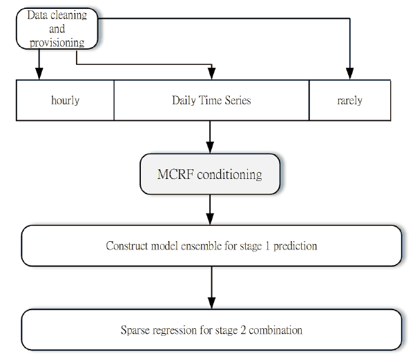
Multiple methods are applied in the ensemble method to maximize the accuracy of prediction and validated on multiple repetition bands for each subspace. This study develops an ensemble of methods in a series of operations, as illustrated in Figure 1.
2.1. Prediction Models in the First Stage
The first stage prediction model f is established to model the functional in (1). Therefore, the functional at time is a function of Y at time t plus a fine-scale, uncorrelated modeling error :
Model f in (2) is an operator that needs to be estimated from the sequence of observation data . The model f can be express by a kernel function and , the i-th component in the functional Y, and
Let , where and are the k-th basis function and coefficient vector in V, respectively. In addition, let . The basis function can be bind to a matrix and the component of kernel function can be bind to a matrix . Therefore, we write (3) to
where and . Estimation of these coefficients in is straightforward in an equivalent Yule-Walker equation [47] or a Nadaraya-Watson kernel estimator [48]. The method of partial least squares can reduce computation time [49]. This study adopts the standard method of partial least squares.
2.2. Learning Ensemble in the Second Stage
Multiple methods are hybridized into an ensemble for each subspace band to ensure that the transformation results are stable. Learners are designed to take either the point day-valued or the functional year-valued precipitation time series from the first stage. To avoid over-fitting during the training phase, the combined regression at the second stage includes all the prediction results from the first stage.
Ensemble prediction modeling is also multi-scaled in the form of discrete wavelet bands. Therefore, individual learners in each band can adapt to the specific data characteristics. Each learner is trained to fit the model matrix , based on the pairs of records in training and testing results of the first stage model (5). The challenge encountered by individual learners during estimation involves the near-singular moment matrix ; this problem is often resolved through regularization by adding a positive perturbation constant or a Lagrange multiplier to the diagonals.
To avoid over-fitting, we further generalized the second stage optimization problem as follows (5) [50].
The optimization (5) is regulated by the Lasso (Least Absolute Shrinkage and Selection Operator) penalty () or the ridge penalty (). The optimization in (5) takes advantage of the norm in evaluating solutions for an ill-posed problem.
Due to the properties of the space, an optimization (e.g., (4)) will minimal non-zero solutions, and it will yield strong reconstruction performance if several sparsity properties, such as restricted isometry and incoherence properties, are satisfied [51,52,53]. In our multivariate transformation matrix , the lasso penalty tends to reduce the coefficients of less important covariates to zero, thus generating more zero solutions and fitting our assumption about the ratio of wet to dry days.
2.3. Markov Chain Random Field Conditioning
In the problem of extreme weather conditions, the coherency among periods of the time series must be established before applying the learning algorithm. Conventional prediction methods rely on the assumption that weather conditions repeat themselves with a certain pattern. Due to the long-memory and fractal properties of precipitation, its occurrence may exhibit similarity in certain subspaces. However, because this repetitive pattern may vary even within the proximal region, the model must be carefully fine-tuned to ensure that the particular realizations of a stochastic process will correctly express the estimation. Increased variation hiders the prediction task under extreme weather conditions. Thus, this study proposes a special method to restore coherency and mitigate the influence of extreme precipitation conditions.
Most statistical approaches establish the model as sampling is performed. Because the process of modeling itself is also an unknown process, some invariant properties could be misguided by a particular pattern of sampling or a realization of precipitation. This sampling variation is mostly observed in high-frequency subspaces or in non-smooth manifolds. A yearly functional time-series can be decomposed into smooth seasonal components and non-smooth stochastic components, which are no-where differentiable manifolds. If the data in these manifolds can be “resample” in certain sense, the prediction consistency can be improved. That is, the validation accuracy will close to the training accuracy. This study utilizes Markov chain random fields (MCRFs) and transiograms to condition the sample values. The transition probabilities of the MCRF are trained based on the entire data history, and the distance lag is defined in the spatio-temporal space. Therefore, MCRF conditioning stabilizes the coherency property, based on the distribution of dry and wet days in the source years on a multi-scale time-frequency decomposition space.
The conditioning method employs the method of MCRF. An MCRF models the spatial dependencies between the vicinity nodes as a Markov chain and applies Bayesian updating to the neighbourhood of a lattice structure. The purpose of MCRF conditioning is to impute missing information over the realizations of the stochastic yearly precipitation. In the subsequent regression steps, the coherence between years may be destroyed by the realizations of random events in the yearly time series. Without conditioning, the predictor may have insufficient information to capture the coherency for the prediction. In this study, the Markov transition probabilities in the MCRF are trained to enhance the accuracy of regression predictors in the functional time series analysis. This conditioning method improves the effectiveness of ensemble learning and accommodates extreme weather conditions.
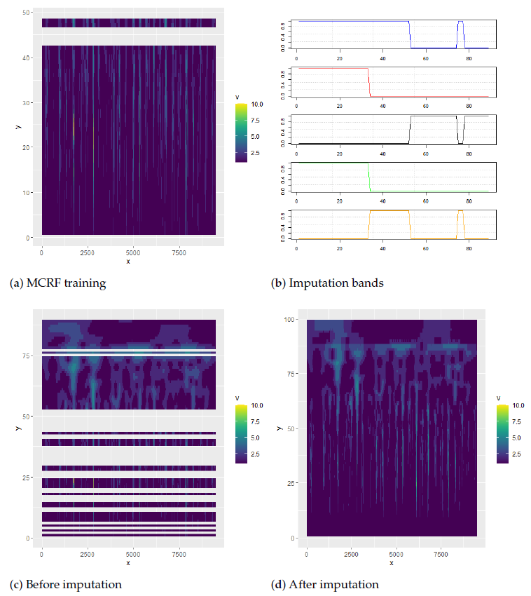
By using MCRF conditioning, the distribution of dry and wet days in the source years is modeled on a multi-scale time-frequency decomposition space. Let be a finite random field on a fixed subset D of a d-dimensional space with state space , in which M nodes reside on the observable manifold and the remaining N unobserved nodes are to be estimated in the unobservable manifold, where . The quantized states over the random field are visualized as shown in Figure 2. Let , for , and let be a symmetric finite hypercube on 𝕊. Then, a probability measure can be defined on the set of Borel -fields as , where is the configuration space of all sequences ; that is, =.
For each , the product measure in 𝕊 is given by , where . The Hamiltonian in is defined as , where is a non-negative potential function on S, and h is a real number that describes gives the strength of an external influence acting at each site in . A control parameter is defined as . The probability measure or finite-volume Gibbs state on is defined as
where is the partition function defined as follows:
From the invariance requirement, it follows that the conditional probabilities
can be determined by parameters. Therefore, the transition matrix can be identified using a conventional machine learning method based on the maximal likelihood algorithm.
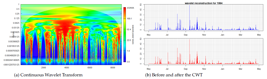
The random field D is designed as a space of multi-scale time-frequency representation, which is obtained from a continuous wavelet transformation (CWT) , with mother wavelets performing dilation in scaling a and shifting t.
The wavelet time-frequency representation reflects the local properties of the time series. For example, the CWT of yearly precipitation clearly exhibits self-similarity in the subspace (Figure 3). The vertical axis in Figure 3 represents the period (frequency) of the CWT in a log scale, starting from the 1-year period at the top to the 1-day period at the bottom.
Figure 2a indicates that the transitional probabilities or transiograms are learned based on wavelet coefficients, which are quantized into discrete intervals and served as the state spaces of each Markov chain of all nodes. We take 60 levels for the quantization. In the control of the balance between a stochastic realization and the MCRF resampling, an imputation mask is provisioned on the ridge curves and the areas of high frequency components, as shown in Figure 2b,c. Due to the semi-periodic nature of storm activities, the ridge amplitudes after imputation are stronger for components in the vicinity of storm seasons, as shown in Figure 2d. Wavelet ridge analysis is used to compute ridge points over the time-frequency representation of a time series . Then, an amplitude ridge point and phase ridge point form a time-scale pair , with a strict local maximum of on the a axis and the t axis. The sets of ridge points collectively form wavelet ridge curves. Notably, Figure 2 shows only the amplitude of the complex numbers for ease of explanation, and the modulus of the complex wavelet coefficients is not shown in the graph.
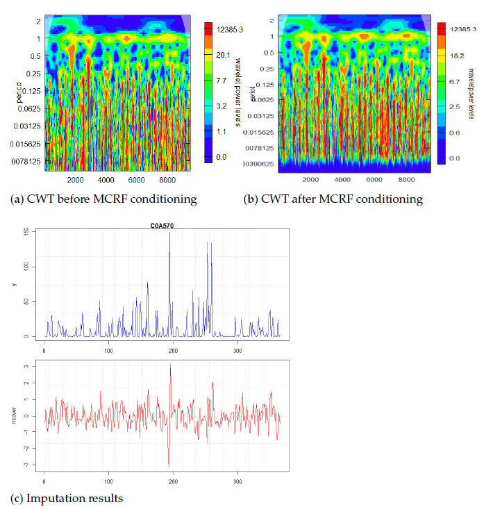
Power spectra are compared in Figure 4, and subgraph (a) shows the original power spectrum in a particular year. Figure 4b shows the imputed result after adding coherence components in the spectrum according to the simulation of the trained transiograms and the sampling masks obtained through ridge analysis. Figure 4c demonstrates and compares the rainfall distribution after MCRF conditioning. The conditioned distribution differs from the original one because the constant trend has been suppressed, and repetitive information from other years has been imputed. Therefore, as shown in the right-hand-side of the Equation (2), has additionally inserted rich information for parameter estimation.
2.4. Data Provisioning
The data source for this study was collected from the Central Weather Bureau (CWB) of Taiwan. From 1994 to 2020, structured data have been recorded at 54 stations across the island (area of 36,193 ). Because a large portion of the territory has high mountains, data collection is difficult in remote areas. Therefore, the recorded data may not be continuous or consistent because stations and equipment may fail or switch in each location. Data cleaning and screening must be performed to provision and populate the data cubes.
Original precipitation data records hourly. The values are aggregated into a daily format. Data from stations with a sufficient number of years of successive data and similar climate conditions are retained in this study. Finally, 26 years of precipitation data from 12 stations are selected for model training. As required for machine learning processes, the data are divided into training and validation sets. Validation is performed based on a hold-out year. Notably, in the validation, high GOF of prediction in the target year and low GOF in non-target years is expected. The functional bandwidth is naturally selected to be 365 days, and each functional is split into three discrete wavelet transform bands for the application of suitable learners for each band.
3. Results and Discussion
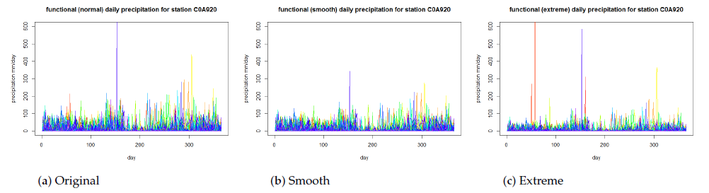
The proposed algorithms are tested using CWB data covering 26 years and 12 stations. In the quantification of the prediction stability for various levels of weather extremity, experiments are designed to verify whether the prediction accuracy drops significantly as the weather extremity is controlled to be increased. For providing a compatible level of comparing experiment, the prediction algorithms are performed for three levels of weather extremity, which are established based on controlled logarithmic and exponential transformations of the raw data. As shown in Figure 5, the original precipitation data are labeled original, and the smooth and extreme precipitation data are logarithmic and exponential transformed, respectively, while maintaining the same level of yearly mean.
Applying MCRF conditioning, as described in (6), significantly improved the prediction accuracy. As shown in Figure 6, MCRF conditioning improved prediction accuracy for not only the training years, but also the validation years. In the ensemble method in the second stage of precipitation prediction modeling, multiple learners are used to combine the intermediate predictions from the first stage, including ordinary generalized matrix inverse, ridge, lasso, and elastic net multivariate regression. For comparison, a deep convolutional neural networks (VGG19 [54]) is also included in the learner ensemble. The experiments demonstrated that the combination of lasso and ridge estimation effectively reconstructed the precipitation time series in the training and validation phases.
Kling–Gupta efficiency (KGE) values are applied to assess the GOF for the developed hydrological models [55,56].
In Equation (9), the statistics between simulated and observed time series are compared and exhibit a tendency of similarity. A positive KGE value is firmly considered acceptable. To meet the goal of year-specific prediction, the notion of KGE is extended to assess GOF over all testing years. We define a difference for a metric in the target year i. This quantity reflects the fact that an accurately targeted prediction must be of high GOF at but of low GOF for all other . Therefore, a high indicates a good prediction for the year i.
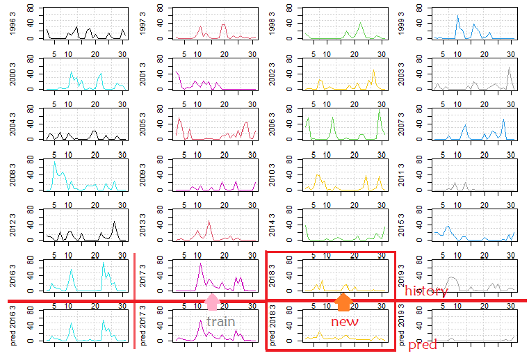
For a water resource manager or a farmer, without our analysis, she only can roughly guess a wide range of precipitation for a large period of time by averaging past several years. For example, in Figure 7, we illustrated March’s daily precipitation from 1996 to 2019. If a water resource manager lives in the beginning of year 2018 and wants to plan for March, she can only ponder the decisions from past experiences without a suitable tool. Looking up the past years, we found that most years had high precipitation at the beginning of March. However, it is challenging to know that when the peak rainfall arrives. Without a tool, it is not easy to make a plan. The manager needs a specific day for planting the crops because a large amount of human resources and machinery need to be booked in advance. Our prediction offers the manager a handy tool to schedule her jobs through a clear prediction of raining amount at each specific date in March.
The last row in Figure 7 showed our predictions. The 2016 and 2017 belonged to the training set, and we list them here only for reference. The prediction performance should look at the accuracy of new data from 2018 and 2019. The data of 2018 and 2019 were pre-excluded from the training set for validation. Therefore, the data of 2018 and 2019 were entirely new to the predictor.
After all testing iterations, the accuracies converged to a stable result for the validation years. Based on the prediction results in Table 1, MCRF conditioning significantly improved the prediction accuracy (KGE) and specificity (KGED) in the proposed two-stage prediction ensemble learning model. The improvement is particularly prominent in the case of extreme weather conditions.
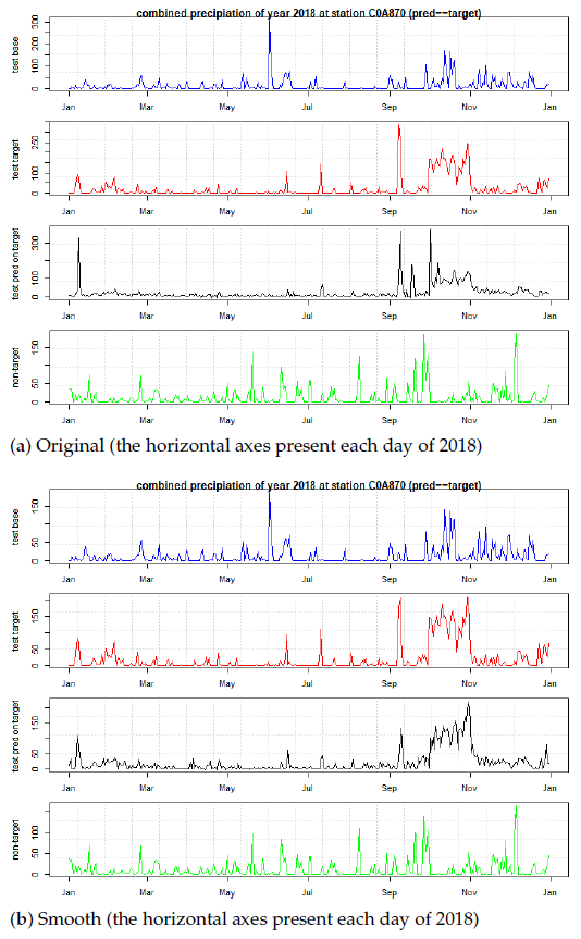
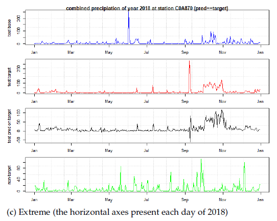
Figure 8 illustrated a prediction result for the proposed ensemble approach. Based on the GOF articulated in Table 1, three predictions are demonstrated in the yearly functional form. The trained model can predict the precipitation of the entire next year. Even in the case of extreme weather conditions, the prediction still maintained robustness without losing statistical details.
Our algorithm is superior to other algorithms because we avoid over-fitting, and the prediction is made specifically for a target year. For example, despite small residuals for the unseen 2018 data, this prediction was still specific for 2018, not for any other years. Our goal of prediction satisfies two criteria: statistical error should be small for the unseen years, and should not close to other years (the error difference between target and non-target years should be large). For one more future year, 2019, consistent with our expectations, the prediction became inaccurate for a longer future. Therefore, the prediction in 2019 is less trustful than expected.
Note also that our algorithm remains consistent even when weather conditions become increasingly extreme. Therefore, in Figure 8c, when weather conditions become extreme, the manager still can rely on the tool to schedule the work without being interfering by weather extremity.
4. Conclusions
This study proposes conditioning and ensemble learning methods to perform forecasting on multi-scaled functional time series over a sparse space. In contrast to other long-range simulations that can yield only a generic rainfall distribution, the proposed long-range prediction method has high yearly-specificity; that is, the performance metric in the present study includes the difference of the GOF of the target year to the GOFs of other years.
The present finding suggests that the MCRF conditioning approach resisted statistical variation due to increasingly extreme weather conditions. The machine learning model accurately predicts the precipitation distribution for the conditioned decomposition in the sparse space. In the results, year-specific accuracy remained high despite increasingly extreme weather conditions. This long-range prediction algorithm may be helpful in certain applications, such as maximizing water usage and increasing yields in agriculture.
Farmers can foresee the precipitation on the planned planting dates. Our tool is even more helpful when the weather conditions become extreme. The difference between with and without the tool reflects on the stability of prediction. The past experiences easily fail at extreme weather. However, we demonstrated that our prediction remains stable when weather conditions become extreme. Therefore, farmers can rely on our method to make their production schedule without being interfering by extreme weather conditions.
Because this study uses conditioning method in conventional kernel model to address the prediction problem of functional time series, the modeling suitability is limited by the Gaussian assumption in the kernel model. We will relax the Gaussian assumption in the future.
Author Contributions
Conceptualization, M.-H.L. and Y.J.C.; methodology, Y.J.C.; software, Y.J.C.; validation, M.-H.L. and Y.J.C.; formal analysis, M.-H.L. and Y.J.C.; investigation, M.-H.L. and Y.J.C.; resources, M.-H.L.; data curation, M.-H.L.; writing—original draft preparation, M.-H.L. and Y.J.C.; writing—review and editing, M.-H.L. and Y.J.C.; visualization, M.-H.L. and Y.J.C.; supervision, M.-H.L.; project administration, M.-H.L.; funding acquisition, M.-H.L. All authors have read and agreed to the published version of the manuscript.
Funding
This research was funded by Ministry of Science and Technology, Taiwan grant number 109-2625-M-020-002 and 109-2410-H-992-018-MY2.
Institutional Review Board Statement
Not applicable.
Informed Consent Statement
Not applicable.
Data Availability Statement
Publicly available datasets were analyzed in this study. This data can be found here: [https://opendata.cwb.gov.tw/dataset/observation/O-A0002-001, accessed on 28 April 2021].
Conflicts of Interest
The authors declare no conflict of interest.
References
- Cowpertwait, P.; O’Connell, P.; Metcalfe, A.; Mawdsley, J. Stochastic point process modelling of rainfall. I. Single-site fitting and validation. J. Hydrol. 1996, 175, 17–46. [Google Scholar] [CrossRef]
- Cowpertwait, P.; O’Connell, P.; Metcalfe, A.; Mawdsley, J. Stochastic point process modelling of rainfall. II. Regionalisation and disaggregation. J. Hydrol. 1996, 175, 47–65. [Google Scholar] [CrossRef]
- Waymire, E.; Gupta, V.K. The mathematical structure of rainfall representations: 1. A review of the stochastic rainfall models. Water Resour. Res. 1981, 17, 1261–1272. [Google Scholar] [CrossRef]
- Waymire, E.; Gupta, V.K. The mathematical structure of rainfall representations: 2. A review of the theory of point processes. Water Resour. Res. 1981, 17, 1273–1285. [Google Scholar] [CrossRef]
- Waymire, E.; Gupta, V.K. The mathematical structure of rainfall representations: 3. Some applications of the point process theory to rainfall processes. Water Resour. Res. 1981, 17, 1287–1294. [Google Scholar] [CrossRef]
- Hughes, J.P.; Guttorp, P.; Charles, S.P. A non-homogeneous hidden Markov model for precipitation occurrence. J. R. Stat. Soc. Ser. C Appl. Stat. 1999, 48, 15–30. [Google Scholar] [CrossRef] [Green Version]
- Bellone, E.; Hughes, J.P.; Guttorp, P. A hidden Markov model for downscaling synoptic atmospheric patterns to precipitation amounts. Clim. Res. 2000, 15, 1–12. [Google Scholar] [CrossRef]
- Ailliot, P.; Thompson, C.; Thomson, P. Space–time modelling of precipitation by using a hidden Markov model and censored Gaussian distributions. J. R. Stat. Soc. Ser. C Appl. Stat. 2009, 58, 405–426. [Google Scholar] [CrossRef]
- Burlando, P.; Rosso, R. Scaling and muitiscaling models of depth-duration-frequency curves for storm precipitation. J. Hydrol. 1996, 187, 45–64. [Google Scholar] [CrossRef]
- De Michele, C.; Kottegoda, N.T.; Rosso, R. The derivation of areal reduction factor of storm rainfall from its scaling properties. Water Resour. Res. 2001, 37, 3247–3252. [Google Scholar] [CrossRef]
- Rinaldi, A.; Djuraidah, A.; Wigena, A.H.; Mangku, I.W.; Gunawan, D. Identification of Extreme Rainfall Pattern Using Extremogram in West Java. In IOP Conference Series: Earth and Environmental Science; IOP Publishing: Bristol, UK, 2018; Volume 187, p. 012064. [Google Scholar]
- Bhatia, U.; Ganguly, A.R. Precipitation extremes and depth-duration-frequency under internal climate variability. Sci. Rep. 2019, 9, 1–9. [Google Scholar] [CrossRef]
- Roderick, T.P.; Wasko, C.; Sharma, A. An improved covariate for projecting future rainfall extremes? Water Resour. Res. 2020, 56, e2019WR026924. [Google Scholar] [CrossRef]
- Dubrovskỳ, M.; Buchtele, J.; Žalud, Z. High-frequency and low-frequency variability in stochastic daily weather generator and its effect on agricultural and hydrologic modelling. Clim. Chang. 2004, 63, 145–179. [Google Scholar] [CrossRef]
- Yao, F.; Müller, H.G.; Wang, J.L. Functional data analysis for sparse longitudinal data. J. Am. Stat. Assoc. 2005, 100, 577–590. [Google Scholar] [CrossRef]
- Paparoditis, E.; Sapatinas, T. Short-term load forecasting: The similar shape functional time-series predictor. IEEE Trans. Power Syst. 2013, 28, 3818–3825. [Google Scholar] [CrossRef] [Green Version]
- Liu, X.; Xiao, H.; Chen, R. Convolutional autoregressive models for functional time series. J. Econom. 2016, 194, 263–282. [Google Scholar] [CrossRef] [Green Version]
- González, J.P.; San Roque, A.M.; Perez, E.A. Forecasting functional time series with a new Hilbertian ARMAX model: Application to electricity price forecasting. IEEE Trans. Power Syst. 2017, 33, 545–556. [Google Scholar] [CrossRef]
- Chen, K.; Delicado, P.; Müller, H.G. Modelling function-valued stochastic processes, with applications to fertility dynamics. J. R. Stat. Soc. Ser. B Stat. Methodol. 2017, 79, 177–196. [Google Scholar] [CrossRef] [Green Version]
- Beyaztas, U.; Yaseen, Z.M. Drought interval simulation using functional data analysis. J. Hydrol. 2019, 579, 124141. [Google Scholar] [CrossRef]
- Mahdi, E.; Provost, S.B.; Salha, R.B.; Nashwan, I.I. Multivariate time series modeling of monthly rainfall amounts. Electron. J. Appl. Stat. Anal. 2017, 10, 65–81. [Google Scholar]
- van Delft, A.; Eichler, M. Locally stationary functional time series. Electron. J. Stat. 2018, 12, 107–170. [Google Scholar] [CrossRef]
- Buffa, A.; Costabel, M.; Sheen, D. On traces for H (curl, Ω) in Lipschitz domains. J. Math. Anal. Appl. 2002, 276, 845–867. [Google Scholar] [CrossRef] [Green Version]
- Tsaig, Y.; Donoho, D.L. Extensions of compressed sensing. Signal Process. 2006, 86, 549–571. [Google Scholar] [CrossRef]
- Ledyaev, Y.; Zhu, Q. Nonsmooth analysis on smooth manifolds. Trans. Am. Math. Soc. 2007, 359, 3687–3732. [Google Scholar] [CrossRef] [Green Version]
- Chen, X. Smoothing methods for nonsmooth, nonconvex minimization. Math. Program. 2012, 134, 71–99. [Google Scholar] [CrossRef]
- Baraniuk, R.G.; Wakin, M.B. Random projections of smooth manifolds. Found. Comput. Math. 2009, 9, 51–77. [Google Scholar] [CrossRef] [Green Version]
- Li, W.; Zhang, C. Markov chain random fields in the perspective of spatial Bayesian networks and optimal neighborhoods for simulation of categorical fields. Comput. Geosci. 2019, 23, 1087–1106. [Google Scholar] [CrossRef]
- Comunian, A.; Renard, P.; Straubhaar, J. 3D multiple-point statistics simulation using 2D training images. Comput. Geosci. 2012, 40, 49–65. [Google Scholar] [CrossRef] [Green Version]
- Strebelle, S. Conditional simulation of complex geological structures using multiple-point statistics. Math. Geol. 2002, 34, 1–21. [Google Scholar] [CrossRef]
- Chugunova, T.L.; Hu, L.Y. Multiple-point simulations constrained by continuous auxiliary data. Math. Geosci. 2008, 40, 133–146. [Google Scholar] [CrossRef]
- Ding, N.; Deng, J.; Murphy, K.P.; Neven, H. Probabilistic Label Relation Graphs with Ising Models. In Proceedings of the IEEE International Conference on Computer Vision, Santiago, Chile, 7–13 December 2015; pp. 1161–1169. [Google Scholar]
- Cerqueira, V.; Torgo, L.; Pinto, F.; Soares, C. Arbitrated Ensemble for Time Series Forecasting. In Proceedings of the Joint European Conference on Machine Learning and Knowledge Discovery in Databases, Skopje, Macedonia, 18–22 September 2017; pp. 478–494. [Google Scholar]
- Mosavi, A.; Ozturk, P.; Chau, K.w. Flood prediction using machine learning models: Literature review. Water 2018, 10, 1536. [Google Scholar] [CrossRef] [Green Version]
- Mosavi, A.; Hosseini, F.S.; Choubin, B.; Abdolshahnejad, M.; Gharechaee, H.; Lahijanzadeh, A.; Dineva, A.A. Susceptibility Prediction of Groundwater Hardness Using Ensemble Machine Learning Models. Water 2020, 12, 2770. [Google Scholar] [CrossRef]
- Arabameri, A.; Chen, W.; Blaschke, T.; Tiefenbacher, J.P.; Pradhan, B.; Tien Bui, D. Gully head-cut distribution modeling using machine learning methods—A case study of nw iran. Water 2020, 12, 16. [Google Scholar] [CrossRef] [Green Version]
- Wei, C.C. Soft computing techniques in ensemble precipitation nowcast. Appl. Soft Comput. 2013, 13, 793–805. [Google Scholar] [CrossRef]
- Zhang, L.; Yang, X. Applying a multi-model ensemble method for long-term runoff prediction under climate change scenarios for the Yellow River Basin, China. Water 2018, 10, 301. [Google Scholar] [CrossRef] [Green Version]
- Ahmed, K.; Sachindra, D.; Shahid, S.; Iqbal, Z.; Nawaz, N.; Khan, N. Multi-model ensemble predictions of precipitation and temperature using machine learning algorithms. Atmos. Res. 2020, 236, 104806. [Google Scholar] [CrossRef]
- Pham, Q.B.; Yang, T.C.; Kuo, C.M.; Tseng, H.W.; Yu, P.S. Combing random forest and least square support vector regression for improving extreme rainfall downscaling. Water 2019, 11, 451. [Google Scholar] [CrossRef] [Green Version]
- Diez-Sierra, J.; del Jesus, M. Subdaily rainfall estimation through daily rainfall downscaling using random forests in Spain. Water 2019, 11, 125. [Google Scholar] [CrossRef] [Green Version]
- Hu, C.; Wu, Q.; Li, H.; Jian, S.; Li, N.; Lou, Z. Deep learning with a long short-term memory networks approach for rainfall-runoff simulation. Water 2018, 10, 1543. [Google Scholar] [CrossRef] [Green Version]
- Miao, Q.; Pan, B.; Wang, H.; Hsu, K.; Sorooshian, S. Improving monsoon precipitation prediction using combined convolutional and long short term memory neural network. Water 2019, 11, 977. [Google Scholar] [CrossRef] [Green Version]
- Lusa, L. Gradient boosting for high-dimensional prediction of rare events. Comput. Stat. Data Anal. 2017, 113, 19–37. [Google Scholar]
- Ferraty, F.; Vieu, P. Nonparametric Functional Data Analysis: Theory and Practice; Springer: Berlin, Germany, 2006. [Google Scholar]
- Greven, S.; Scheipl, F. A general framework for functional regression modelling. Stat. Model. 2017, 17, 1–35. [Google Scholar] [CrossRef]
- Aneiros-Pérez, G.; Cao, R.; Vilar-Fernández, J.M. Functional methods for time series prediction: A nonparametric approach. J. Forecast. 2011, 30, 377–392. [Google Scholar] [CrossRef] [Green Version]
- Masry, E. Nonparametric regression estimation for dependent functional data: Asymptotic normality. Stoch. Process. Their Appl. 2005, 115, 155–177. [Google Scholar] [CrossRef] [Green Version]
- Beyaztas, U.; Shang, H.L. On function-on-function regression: Partial least squares approach. Environ. Ecol. Stat. 2020, 27, 95–114. [Google Scholar] [CrossRef] [Green Version]
- Zou, H.; Hastie, T. Regularization and variable selection via the elastic net. J. R. Stat. Soc. Ser. B Stat. Methodol. 2005, 67, 301–320. [Google Scholar] [CrossRef] [Green Version]
- Candes, E.J.; Tao, T. Decoding by linear programming. IEEE Trans. Inf. Theory 2005, 51, 4203–4215. [Google Scholar] [CrossRef] [Green Version]
- Candès, E.J.; Romberg, J.; Tao, T. Robust uncertainty principles: Exact signal reconstruction from highly incomplete frequency information. IEEE Trans. Inf. Theory 2006, 52, 489–509. [Google Scholar] [CrossRef] [Green Version]
- Candes, E.J. The restricted isometry property and its implications for compressed sensing. Comptes Rendus Math. 2008, 346, 589–592. [Google Scholar] [CrossRef]
- Simonyan, K.; Zisserman, A. Very deep convolutional networks for large-scale image recognition. arXiv 2014, arXiv:1409.1556. [Google Scholar]
- Pool, S.; Vis, M.; Seibert, J. Evaluating model performance: Towards a non-parametric variant of the Kling-Gupta efficiency. Hydrol. Sci. J. 2018, 63, 1941–1953. [Google Scholar] [CrossRef]
- Knoben, W.J.; Freer, J.E.; Woods, R.A. Inherent benchmark or not? Comparing Nash–Sutcliffe and Kling–Gupta efficiency scores. Hydrol. Earth Syst. Sci. 2019, 23, 4323–4331. [Google Scholar] [CrossRef] [Green Version]
Figure 1.
Two-stage prediction and conditioning.

Figure 2.
Quantized spectral maps. Because Markov chains take categorical values, the CWT must be quantized to levels. (a) The target transiogram extracted from training datasets (X represented time point, Y represented frequency). (b) Imputation bands specified how MCRF performed for each frequency (The top one had the lowest sampling density on the mask, and the bottom one had the highest sampling density on the mask. The horizontal axis represented frequency). (c) The transiogram masked by the imputation bands. (d) the imputed transiogram by MCRF.

Figure 3.
Local properties of a time series in its time-frequency representation. (a) The vertical axis represents the period (frequency) of the CWT in a log scale, starting from the 1-year period at the top to the 1-day period at the bottom. (b) The CWT reserves the original time series after reconstruction from the transformation in (a).

Figure 4.
Given a time series, the CWT before the MCRF (a) and after the MCRF conditioning (b) shows a minor imputation on the time-frequency representation. The coherent components are restored to the spectrum according to the simulation of the trained transiograms and the sampling masks obtained through ridge analysis. (c) The comparison of two time series manifests the difference of MCRF conditioning. The blue graph is the original, and the red graph is the reconstructed components. The red line had been imputed additional extreme events according to the history of the time series. The low frequency mean-value in the blue line had been removed for the red line. The vertical scales play no roles in this stage because the red graph is only an intermediate coefficient and will be rescaled to other scales.

Figure 5.
Data provision for three variations in daily precipitation at a weather station over 26 years. (a) The original time series. (b) The time series in logarithmic transformation. (c) The time series in exponential transformation.
Figure 5.
Data provision for three variations in daily precipitation at a weather station over 26 years. (a) The original time series. (b) The time series in logarithmic transformation. (c) The time series in exponential transformation.

Figure 6.
An example of the prediction results for training and validation sets with MCRF conditioning. From the qualitative point of view, the result demonstrated good predictability but not over-fitted from training data to validation data. Through the rough comparison, a certain degree of errors exists is necessary for future uncertainty.

Figure 7.
Row 1 to Row 4: Historical data for March’s daily precipitation from 1996 to 2019. Row 5: Prediction results from 2016 to 2019. Old training set: 1996 to 2017. New validation set: 2018 to 2019. A water resource manager lives in the beginning of year 2018 and obtains the prediction in March 2018. The daily amount of prediction can be a basis for her usage planning.

Figure 8.
Subgraphs (a–c) show the stability under extremity. The validation were from 2018 to 2019 for three levels of weather extremity. The 2018 and 2019 were pre-excluded from training data and were entirely new to the predictor. Vertical axes are daily precipitation in mm/day and horizontal axes are date. The top and the second panel is the time series of current year (2018, in blue color), the next year (2019, in red color), respectively. The third panel is the predicted time series of the target year (2019, in black color). The fourth panel is merely a time series of a non-target year (2020, in green color). Together with Table 1, the graphs demonstrate that the prediction is accurate for 2019 (the third is similar to the second) but not for 2020 (the third is not similar to the fourth). Even the weather condition becomes extreme, the prediction and KGE in (c) still remains accurate for 2019.


Table 1.
Prediction accuracies for the validation years.
| Metrics | Extremity | Before MCRF | After MCRF |
|---|---|---|---|
| KGE | normal | 0.65 | 0.68 |
| KGE | smooth | 0.73 | 0.74 |
| KGE | extreme | 0.40 | 0.58 |
| KGED | normal | 1.22 | 1.29 |
| KGED | smooth | 1.14 | 1.16 |
| KGED | extreme | 1.10 | 1.27 |
MCRF = Markov Chain Random Field, KGE = Kling–Gupta Efficiency, KGED = KGE Difference.
Publisher’s Note: MDPI stays neutral with regard to jurisdictional claims in published maps and institutional affiliations. |
© 2021 by the authors. Licensee MDPI, Basel, Switzerland. This article is an open access article distributed under the terms and conditions of the Creative Commons Attribution (CC BY) license (https://creativecommons.org/licenses/by/4.0/).
Share and Cite
MDPI and ACS Style
Lee, M.-H.; Chen, Y.J. Precipitation Modeling for Extreme Weather Based on Sparse Hybrid Machine Learning and Markov Chain Random Field in a Multi-Scale Subspace. Water 2021, 13, 1241. https://doi.org/10.3390/w13091241
AMA Style
Lee M-H, Chen YJ. Precipitation Modeling for Extreme Weather Based on Sparse Hybrid Machine Learning and Markov Chain Random Field in a Multi-Scale Subspace. Water. 2021; 13(9):1241. https://doi.org/10.3390/w13091241
Chicago/Turabian StyleLee, Ming-Hsi, and Yenming J. Chen. 2021. "Precipitation Modeling for Extreme Weather Based on Sparse Hybrid Machine Learning and Markov Chain Random Field in a Multi-Scale Subspace" Water 13, no. 9: 1241. https://doi.org/10.3390/w13091241
Note that from the first issue of 2016, this journal uses article numbers instead of page numbers. See further details here.