
Cyber—Physical Attack Detection in Water Distribution Systems with Temporal Graph Convolutional Neural Networks


Department of Water Resources and Environmental Engineering, School of Civil Engineering, National Technical University of Athens, Iroon Politechniou 5, Zografou, 157 80 Athens, Greece
*
Author to whom correspondence should be addressed.
Water 2021, 13(9), 1247; https://doi.org/10.3390/w13091247
Submission received: 26 March 2021
/
Revised: 26 April 2021
/
Accepted: 27 April 2021
/
Published: 29 April 2021
(This article belongs to the Section Urban Water Management)
Abstract
:Prompt detection of cyber–physical attacks (CPAs) on a water distribution system (WDS) is critical to avoid irreversible damage to the network infrastructure and disruption of water services. However, the complex interdependencies of the water network’s components make CPA detection challenging. To better capture the spatiotemporal dimensions of these interdependencies, we represented the WDS as a mathematical graph and approached the problem by utilizing graph neural networks. We presented an online, one-stage, prediction-based algorithm that implements the temporal graph convolutional network and makes use of the Mahalanobis distance. The algorithm exhibited strong detection performance and was capable of localizing the targeted network components for several benchmark attacks. We suggested that an important property of the proposed algorithm was its explainability, which allowed the extraction of useful information about how the model works and as such it is a step towards the creation of trustworthy AI algorithms for water applications. Additional insights into metrics commonly used to rank algorithm performance were also presented and discussed.
1. Introduction
In an era of unprecedented technological advancements, the water sector is undergoing a digital transformation [1]. Digital devices have already been deployed in water distribution networks (WDNs) to monitor and control utility operations, and to increase the network’s automation and efficiency, and although water digitalization is essential, it comes at a cost: It exposes the WDN to the risks of a cyber–physical system, i.e., cyber-attacks [2]. Since the impact of a potential attack could be enormous [3], research interest on the security of water infrastructures is growing [4]. In the face of a potential cyber-attack, one of the emerging fields of ongoing research focuses on the early detection of attacks [5]. Prompt detection of cyber–physical attacks is a prerequisite to respond to the threat swiftly and avoid irreversible damages, but it is a task that is arguably challenging due to the nature of WDN’s fluxes (e.g., water demand, pipe pressure). WDN’s fluxes are governed by stochasticity and high variability [6], characteristics that imply that researchers should treat them as realizations of stochastic processes [7].
Attack detection algorithms on water distribution networks generally rely on Supervisory Control and Data Acquisition (SCADA) system data to classify the system as safe or under attack. SCADA data are real-time, field-based network measurements (tank water level, pump flow, etc.) transmitted to the central system by programmable logic controllers (PLCs). A key characteristic of SCADA data is that they have spatiotemporal interdependencies. In theory, an algorithm that effectively captures these complex interdependencies would be able to detect intrusions even when they are concealed by the attacker [8]. Tuptuk et al. [4] divided cyber–physical systems’ attack detection algorithms into three categories: Model-based, machine learning, and statistical methods. Each method processes the spatiotemporal attributes of the data differently.
Model-based methods, such as the one proposed by Housh and Ohar [9], attempt to model the physical process of the system and therefore account simultaneously for the spatial and temporal information of the network with a single model. However, model-based methodologies are difficult to implement in real-life settings, because a well-calibrated hydraulic model of the network is often unavailable. On the contrary, statistical models ignore the spatiotemporal information of the data and are often used in combination with machine learning models to create multi-stage algorithms [10,11,12].
Machine learning methods do not process the spatiotemporal information in a specific way; rather, it depends on the proposed model. Temporal information is often processed by modeling the SCADA data as time series data [12,13]. Brentan et al. attempted to go a step further and add the time of the day as an input feature to their model [10], while Kadosh et al. followed a completely different route and created different models for each hour of the day [14]. Most researchers use the spatial relations of the SCADA data only as a guide to group nearby features and to create different models for different sub-areas of the network [10,13,14,15]. Some machine learning models ignore entirely the spatial and temporal context of the SCADA data [12,15,16,17,18]. However, in the case of the autoencoder proposed by Taormina et al., the authors argued that their model accounts implicitly for the spatial and temporal information, as this information is reflected in the SCADA data [16].
So far, there have been no machine learning models reported in the relevant literature that explicitly embed in their architecture the spatial information of SCADA data. As a result, a unifying approach that simultaneously encompasses temporal and spatial relationships has not been proposed to date. Meanwhile, there has been a rapid development of deep learning models that operate on relational data (i.e., graphs) called graph neural networks (GNNs). GNNs have been used successfully in many similar time series problems like traffic forecasting [19], motion recognition [20], and automatic seizure detection [21]. For that reason, we speculated that they might perform well in attack detection problems.
In this work, we propose a prediction-based CPA detection algorithm that leverages the inherent interdependencies of the SCADA data through temporal graph convolutional neural networks (TGCN) [21] and makes use of the Mahalanobis distance. Our goal was to explore whether the inherent ability of a TGCN to incorporate the relationships between the nodes of a graph makes it a valuable tool in CPA detection and localization. We examined whether the model was able to learn a meaningful representation of the network and attempt to understand how the model localized attacks by employing a simple removal-based explanation method. To develop and evaluate our algorithm, we used the publicly available datasets featured in the battle of the attack detection algorithms (BATADAL) competition [5]. The proposed algorithm displayed a strong detection performance, equivalent to the best-performing models developed for that competition, while also presenting a unique combination of advantages that are further discussed below.
2. Materials and Methods
2.1. Temporal Graph Convolutional Networks
A temporal graph convolutional network [21] is a deep learning model that operates on a structural time series by performing localized feature extraction shared both in space and time. A structural time series has the form where contains -dimensional observations across time steps for different sequences and is the adjacency matrix of the p sequences. The adjacency matrix can be symmetric for undirected graphs or asymmetric for directed graphs, and has 1s in its diagonal.
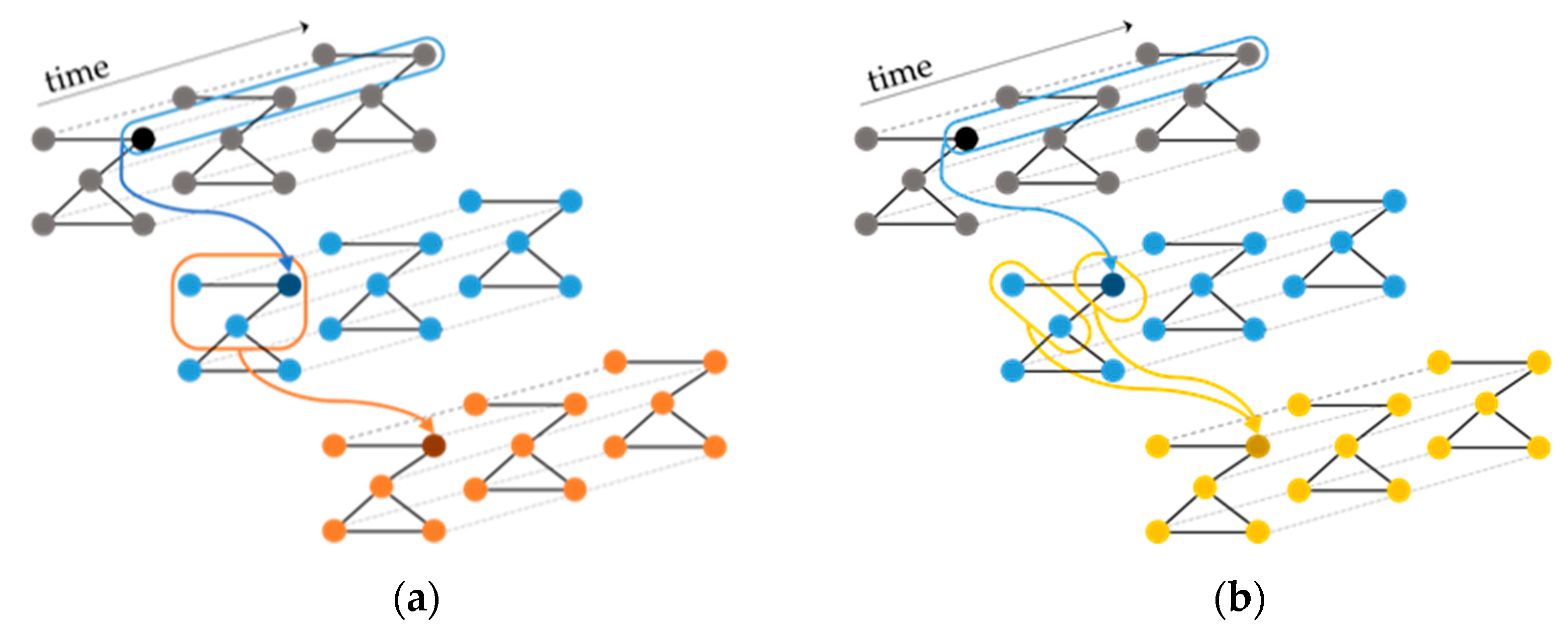
A TGCN consists of several spatio-temporal convolutional (STC) layers [21] that operate on the input sequences in a way that allows the graph topology to be maintained at each layer. The STC layer applies a 1D convolution to each of its input sequences and then refers to the adjacency matrix of the structural time series to aggregate neighboring features. The STC layer can be used with two different aggregation rules: Rule A aggregates features from the node’s neighborhood including the node itself and Rule B aggregates features from the node’s neighbors, and then combines these features with the node’s own features (Figure 1).
Covert et al. define the two rules as follows:
Rule A:
Rule B:
where is the input to the layer with number of time points and represents the hidden features associated with sequence of the input, denotes the 1D convolution with filter , and a nonlinearity. The neighborhood of node is defined as and represents the set of nodes that are within steps reachable to .
is the k-step reachability matrix obtained from the operation where is the graph’s adjacency matrix to the kth power and is an element-wise indicator function. Setting enables information to spread through the graph using fewer layers.
The only parameter for Rule A is the convolutional kernel . Rule B has two parameters: , and the second convolutional kernel . Note that the number of parameters of an STC layer are independent to the input adjacency matrix. This property allows the TGCN model to accept inputs with arbitrary graph topologies, and therefore, facilitates the use of removal-based explanations to interpret the model predictions.
2.2. Attack Detection Algorithm
The aim of an attack detection algorithm is to successfully classify the system’s state as “safe” or “under attack” at all times. However, approaching the problem with binary classification techniques is unrealistic, as in practice, a dataset with a sufficient and diverse set of labeled attacks is usually unavailable. Relying on statistic and regression techniques, instead, seems more promising in our case, because there are plenty of data representing the system under normal operating conditions.
Since the goal was to approach the attack detection problem with a TGCN model, we started by representing the water network as a mathematical graph where its nodes (tanks, junctions, and pumps) were linked with edges (pipes). Then, we could define the SCADA readings as structural time series that have the form where contains -dimensional observations across time steps for different nodes and is the adjacency matrix of the nodes of the network. By representing the SCADA data as structural time series, we could then use them as inputs to a TGCN model and train it for a specific task.
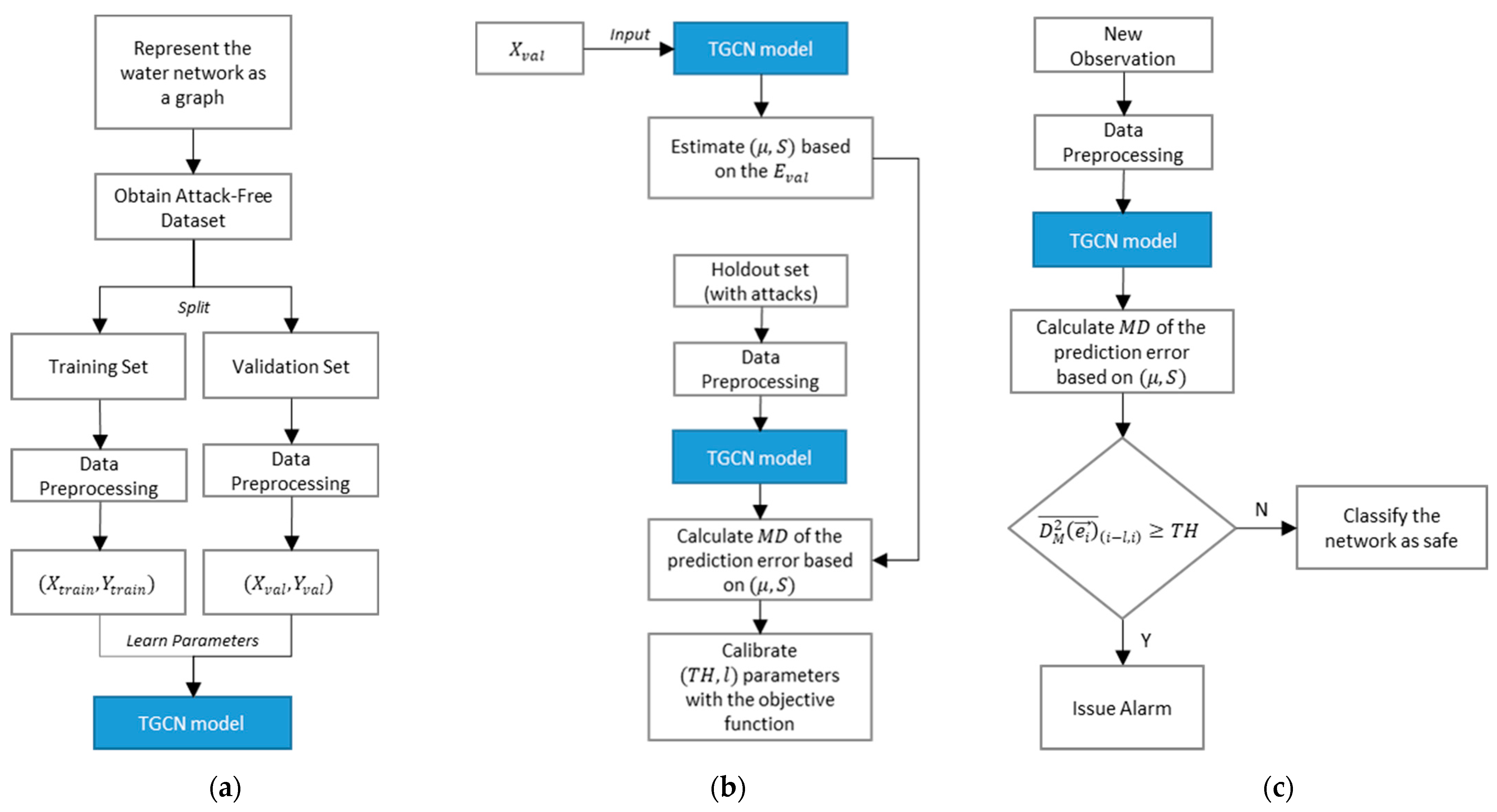
The proposed attack detection algorithm was developed: (a) First by training a TGCN model that predicted the current SCADA measurements, and then (b) by calibrating an attack detection scheme that issued alarms based on the comparison of the predicted values with the observed.
2.2.1. TGCN for Time-Series Prediction
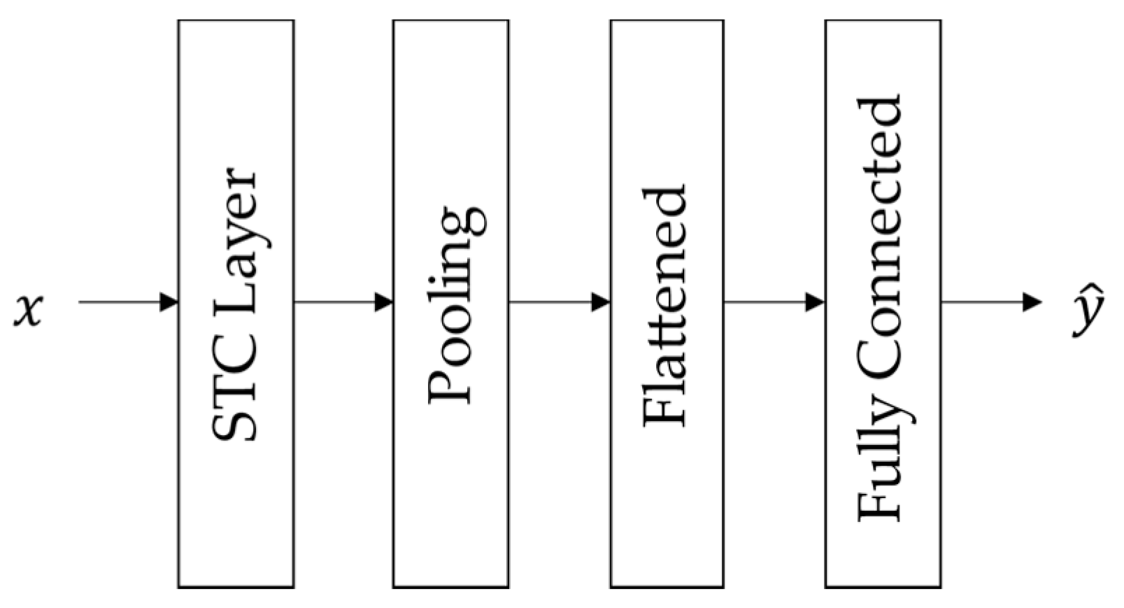
The first step of the attack detection algorithm required training a TGCN model that predicted the current network observations, given the SCADA measurements of prior timesteps. The basic structure of the TGCN model, as we implemented it, consists of one or more STC layers, each one followed by a pooling layer along the temporal dimension. Then, the output of the last STC layer is flattened and passed to a fully connected neural network to make predictions (Figure 2).
To learn a representation of the network under normal operating conditions, the model requires an event-free dataset (i.e., with no attacks) split into training ( and validation (. Before training the TGCN model and as a preprocessing step, the data were scaled such that the maximal absolute value of each feature in the training set would be . To obtain subsequences and use them as inputs to the model, we took a window of a fixed size and slid it over the time series with a step size . The first measurements of each window were the input to our model, while the final, observations were the target output.
2.2.2. Calibration of the Attack Detection Scheme
After TGCN was trained, the validation set was passed through the model to make a prediction . We defined as the prediction error , the difference between the actual observations and the predictions for each timestep.
Since there are not attacks in either the training or in the validation set, we assumed that the prediction error at each node was roughly Gaussian distributed. Hence, we could estimate the parameters () of a multivariate Gaussian distribution that describes the model’s prediction error under normal operating conditions, where is the covariance matrix and is the mean vector of the validation prediction errors .
Given the model’s prediction error at timestep , , we could compute its distance from the mean vector of the multivariate Gaussian distribution using the Mahalanobis distance (MD). The squared Mahalanobis distance is defined as:
Note that is essentially the sum of independent standard normal variables, and for that reason, follows a chi-squared distribution with degrees of freedom [22].
There were two reasons why we chose the squared MD as an anomaly score for our algorithm. First of all, the MD incorporates the dependencies between the prediction errors at each sensor. This is a useful property when the goal is to detect not only nodes with unusually high prediction errors, but also unusual prediction error combinations. The second reason was that issuing alarms based on the MD was more straightforward, as it only required us to tune one global anomaly threshold, instead of multiple thresholds that were equal to the number of the network’s nodes.
Our expectation was that normal observations would have lower MD values compared to anomalous instances. However, before defining a cutoff criterion to separate normal from anomalous instances, we calculated the rolling mean of the raw anomaly scores to avoid false positives. An alarm was issued at timestep , when:
where is the mean of the squared MD in a window of length ; and is the cutoff threshold. Selecting and requires a calibration procedure. The procedure is done numerically by testing different values for the two parameters in a holdout set with a few positive examples (attacks) and calculating the algorithm’s performance with the appropriate objective function. The objective function should reflect the algorithm’s performance in detecting attacks. The parameter values that maximize the objective function can then be used in new, unseen by the algorithm datasets to evaluate its performance (Figure 3).
3. Case Study
3.1. BATADAL
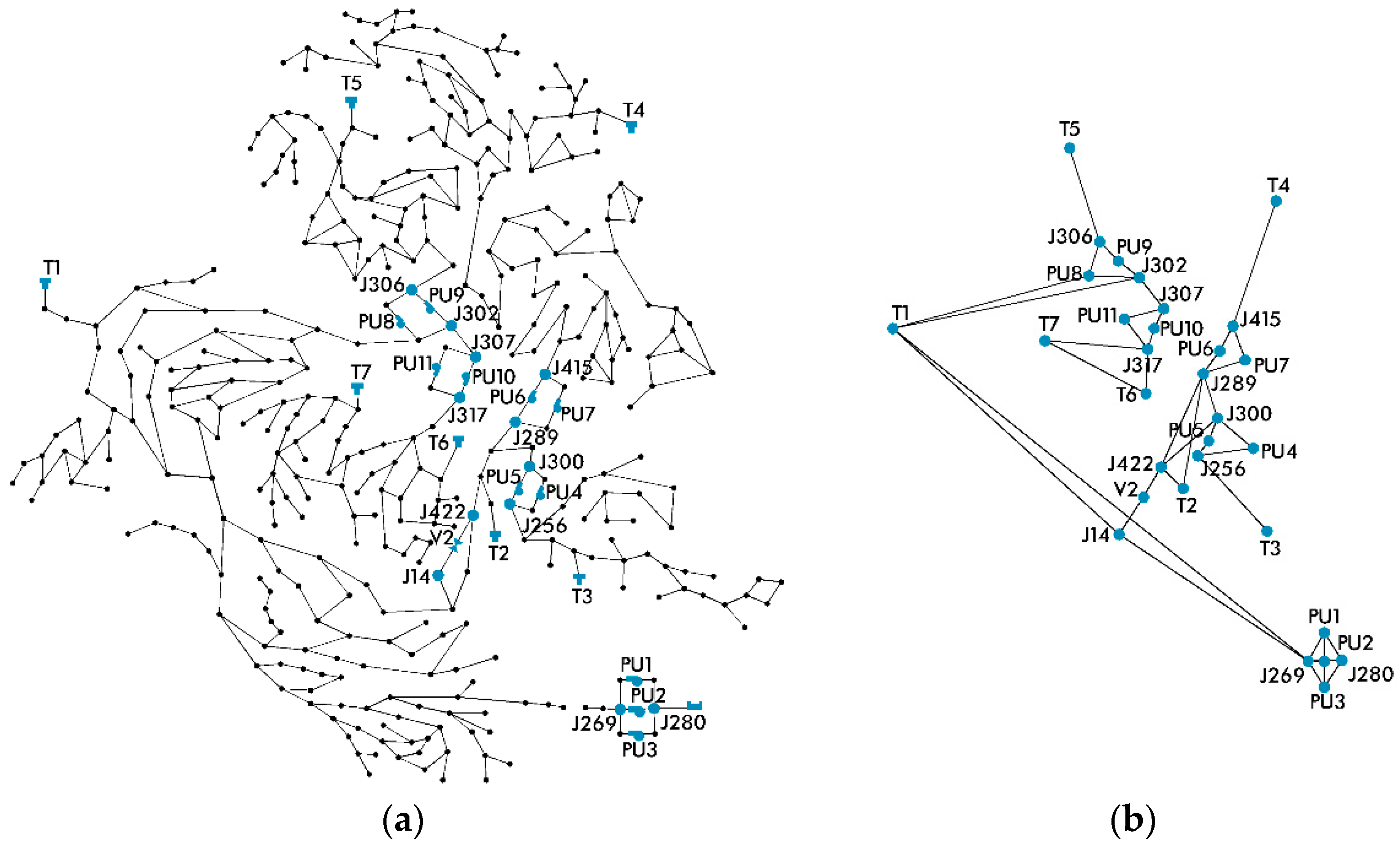
Our algorithm was trained and tested using the datasets featured in the battle of the attack detection algorithms, an international competition in cyber-security of water distribution systems. In BATADAL, the contestants were given three datasets containing hourly SCADA measurements of a medium-sized real network, named C-Town. C-Town consists of 388 nodes linked with 429 pipes and is divided into 5 district metered areas (DMAs). The goal was to create an algorithm that detects when C-Town is under attack.
Each of the three datasets provided at the competition contains 43 sequences of SCADA measurements from 31 different variables of the network. More specifically, the SCADA data include the water level at all 7 tanks of the network (T1–T7), status and flow of all 11 pumps (PU1–PU11) and the one actuated valve (V2) of the network, and pressure at 24 pipes of the network that correspond to the inlet and outlet pressure of the pumps and the actuated valve.
The first dataset () contains 12 months of observations and represents the network under normal operating conditions (i.e., it is attack-free). The other two datasets ( and ) have durations of 6 and 3 months, respectively, and contain 7 attacks each. All datasets were simulated using epanetCPA [8]. To develop their models, the contestants were initially given only , and a semi-labeled version of (we denote it as ) that contains only one attack fully labeled and the remaining partially revealed or hidden. The algorithms were later ranked based on their performance on . We should also note that most of the attacks in and were concealed. This means that the attacker had modified some of the SCADA observations in an attempt to conceal the actual impact on the network.
The BATADAL contest and the attack scenarios of and are described in detail by Taormina et al. [5].
3.2. Application of the Attack Detection Algorithm to C-Town
As a first step, we constructed C-Town’s adjacency matrix. Given that the available measurements were only from 31 of the network’s nodes, it was not possible to use the adjacency matrix of the whole network. As a result, we created a new, condensed adjacency matrix that described the connections only between the nodes whose observations were available (Figure 4). For each node of the condensed network, only one measurement was reported. The only exceptions were the pump nodes that reported two different measurements: Status and flow. Since all nodes should have the same number of measurements, we excluded the pump status, which is a binary variable, and we kept the numerical flow rate.
For the development of our model, we used the attack-free and split it into training and validation in a 75:25 ratio. To learn the prediction task, the TGCN architecture included three stacked STC layers with output channels, respectively, and a temporal kernel . Each STC layer was followed by a max pooling layer. Finally, the output of the last STC layer was flattened and passed to a fully connected layer with 128 neurons and then its output was passed to a final linear layer to attain a forecast for the network’s current measurements. The STC layers used as their aggregation rule and the 3-step adjacency matrix of the network We used ReLu as an activation function. The model was trained with subsequences of length ( taken in mini-batches of size from the training inputs and targets . During training, we used the Adam optimizer to minimize the mean squared error (MSE) loss. Early stopping was applied to prevent overfitting of the model and to reduce the overall time required for the training process. All hyperparameters were experimentally chosen based on effective models, meaning that other optimal values could be possible.
3.3. Algorithm Performance Metrics
To evaluate our algorithm’s performance, we mainly used two performance metrics: the score and the score.
The score is a metric used in BATADAL to evaluate the CPA detection algorithms, and it is a combination of two different metrics into one.
The first metric is time to detection:
where number of attacks, and the time to detection of attack as a ratio of the total attack duration .
The second metric is classification performance which is defined as:
where True Positive Rate , and True Negative Rate .
The two metrics are combined into a single score:
where , which means that for the competition both metrics were considered equally important.
Note that the score implements TNR to determine the model’s ability to avoid false alarms. The drawback of TNR in imbalanced classification datasets, like the ones in attack detection, is that TNR determines true negatives as more important than true positives. True negatives (safe conditions) in anomaly detection problems are the majority class of the datasets; thus, TNR presents small variance and makes it hard to capture the differences in an algorithm’s performance in terms of the number of false positives it issues.
score is the weighted harmonic mean of precision and recall:
where is the model’s ability to avoid false alarms, (or TPR) measures the algorithm’s ability to identify when the system is under attack, and determines the balance between precision and recall, with high values favoring recall.
For the score is called the score and considers equally recall and precision. Other common variations of score are the score, which deems recall as twice as important as precision, and , which in the exact opposite way, deems precision as twice as important as recall.
The advantage of the score is that it gives focus to true positives, false positives, and false negatives, while no attention is given to the majority class, i.e., the true negative group. However, when it is used as a single-score metric, the main shortcoming resides in the fact that low recall from low precision models cannot be distinguished.
4. Results
4.1. Attack Detection Performance
We trained the TGCN model 20 times using the attack-free , and for each TGCN model, we fine-tuned the detection rule parameters using as a holdout set, , and as an objective function the maximization of score on the holdout set. The average performance of the TGCN model on the test set () across 20 trainings is and the low variance of the score indicates that the algorithm tends to have a consistent performance between different training instances. To gain more insight on how the algorithm performs, we present the results of the best model, which was selected based on its performance on the holdout set ().
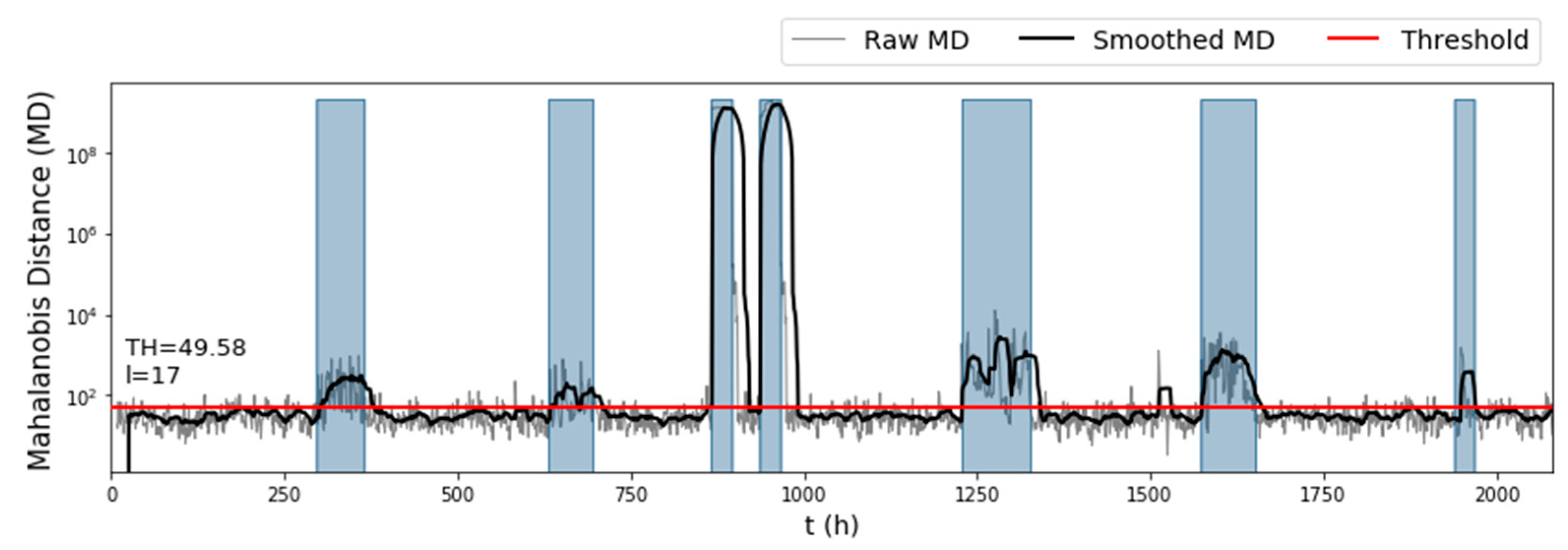
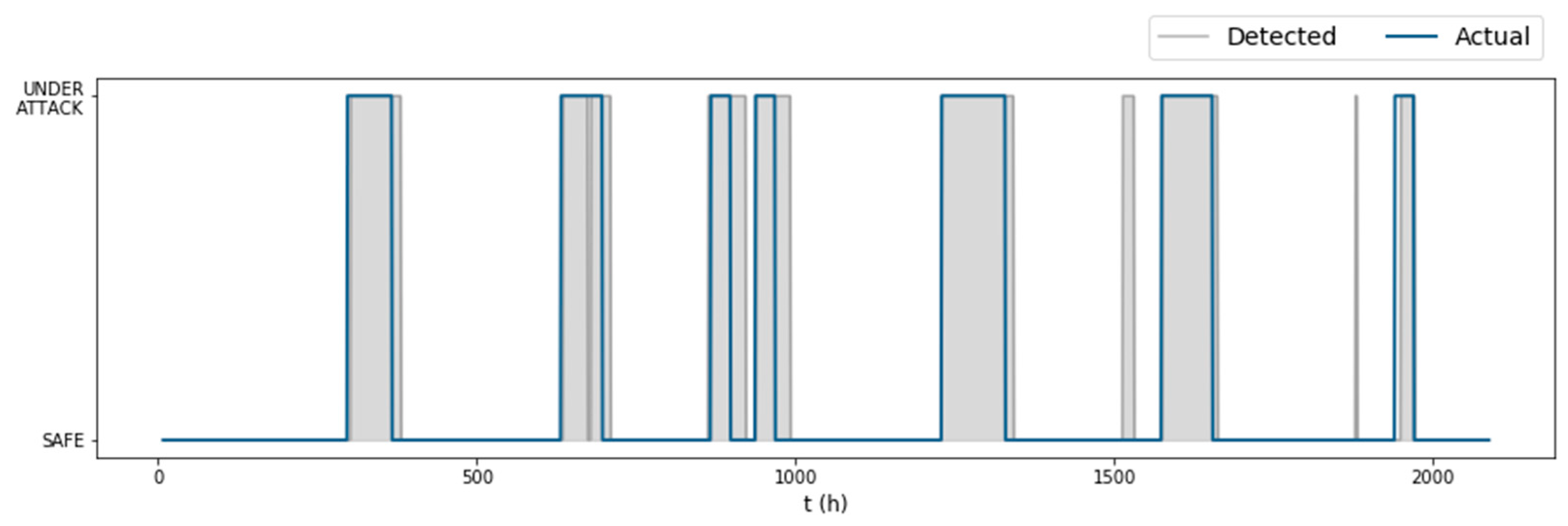
Judging only by the raw anomaly scores of the test set (Figure 5), we expected that the algorithm would perform well on the test set, due to the obvious increase of the MD when the network was under attack. Indeed, when the detection rule was applied, the algorithm detected all seven attacks of the test set, together with two false alarm instances (Figure 6). The parameters selected by the fine-tuning process were This large length of the rolling mean window offset the alarms issued by the algorithm and as a result improved the true positive rate on the dataset, but it was also the reason why so many false positives were issued after some attacks ended. Only 16% of the total false positives corresponded to false alarm instances. The first false alarm lasted 17 hours (between the fifth and sixth attack), and the second had only a 2-hour duration (between the sixth and seventh attack). The detection times of each attack were , resulting in a time to detection score that combined with the gave the algorithm an overall on the test set.
When it comes to the running time of the proposed algorithm, the majority of the computational load was consumed at the training stage of the TGCN. After the development of the model and when the attack detection scheme was applied to new observations, the runtime was sufficiently fast, as it took a few seconds. Especially in the BATADAL datasets, where the observations are reported on an hourly timescale, the algorithm’s runtime did not affect the evaluation process.
4.2. Sensitivity Analysis
Training the TGCN model is a non-deterministic process and the results depend on factors such as the initial starting point and batch randomization. When we trained our algorithm multiple times, we noticed that its performance metrics had a small variance between different training instances, indicating that the TGCN was fairly stable. However, the proposed attack detection algorithm also involved the calibration of the detection rule parameters , a process that relies on the holdout set (one preferably with labeled attacks) and the objective function. In this section, we explore how different data availability scenarios and the choice of the objective function affected the algorithm’s performance.
4.2.1. Data Availability
The proposed algorithm was trained using data under normal operating conditions and then the detection rule parameters and were selected in a supervised way using the fully labeled . However, fully labeled datasets with attacks are limited in practice. For that reason, we examined the algorithm’s performance under two different data availability scenarios. More specifically, we fine-tuned the detection rule parameters using:
- : The semi-labeled version of that was given initially to the BATADAL contestants for algorithm development “corresponds to a postattack scenario in which forensics experts carry out an investigation to determine whether, when and where the water distribution system has been affected” [5];
- : We investigated the scenario where a dataset containing attacks was unavailable. We used as a holdout set the validation set ( and since it does not contain attacks, we could not use the aforementioned objective functions that were tailored to binary classification datasets. Nevertheless, the squared Mahalanobis distance follows a chi-squared distribution with degrees of freedom. Hence, we set equal to the upper-tail critical value of chi-squared distribution with degrees of freedom at a significance level. Then, the length of the mean rolling window was calibrated by minimizing the number of false alarms in the validation set.
The algorithm was able to detect all attacks in the test dataset under different data availability scenarios and to retain its performance in terms of the score (Table 1). Perhaps this indicates that the attack detection algorithm can also be employed in a completely unsupervised way, without the need of a set with labeled attacks. However, since the results concerned the algorithm’s performance only on , we need to further test our hypothesis before drawing a conclusion.
4.2.2. Objective Function Choice
When tuning the detection rule parameters , the goal was to select a combination such that the attack detection algorithm would detect as many attacks as possible while issuing a small number of false alarms. Ideally, having available a single-number metric that is closely tied with these objectives can significantly speed up the developing process. However, we noticed that using as an objective function the maximization of the score on the hold-out set () often resulted in a selection that produced many false positive instances. Given that optimizing the algorithm’s detection performance on the holdout set precedes its evaluation on unknown test sets, we decided to explore how different objective functions perceive the algorithm’s performance as “optimal”. For that reason, we experimented with replacing the score from the objective function with and score, and our findings are presented below.
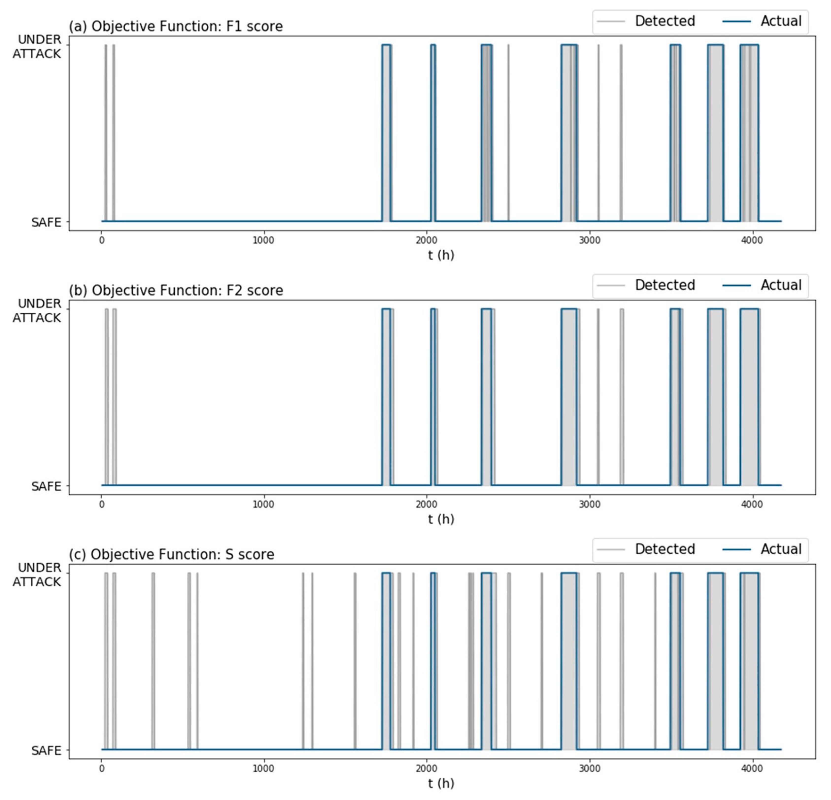
Figure 7 and Table 2 show the performance of our algorithm on the holdout set ) for the same TGCN model, but for different objective functions. From the examples, we observed that changing the objective function could lead to algorithms that produce fewer false positives without compromising the attack detection performance. Notice how in this example, algorithms (b) and (c) had roughly the same score (Table 2) and yet, algorithm (c) issued a lot more false alarms (Figure 7). This is because the score implements TNR to determine the model’s ability to avoid false alarms, which presents small variance in imbalanced datasets. As a result, using the score in the objective function (which also prioritizes the detection of attacks) produced fewer false positive instances (Figure 7) without compromising the attack detection performance (Table 2).
A common issue among the metrics in question is that they consider false positives as independent from each other. However, scattered false positives contribute to the “crying wolf” effect, while the same number of false positives concentrated one after the other can be viewed as a single false alarm. This is especially highlighted when looking at the number of false positives issued by the algorithms tuned with and score (algorithm (a) and (b), respectively) (Table 2). We would expect that algorithm (a), which issued fewer false positives than algorithm (b), would also issue fewer false alarm instances. Nevertheless, algorithm (a) issued five false alarm instances and algorithm (b) four (Figure 7).
Although the score was reasonably designed to be biased towards attack detection (like score), it failed to distinguish when an algorithm issued too many false positives and as a result sometimes failed to rank the performance of different algorithms. This was especially challenging at the developing stage where is used to solve an optimization problem. We argue that to accelerate the development of threshold-based algorithms, there is a need to adopt common performance metrics that are better aligned to the challenge of cyber–physical attack detection in water distribution networks.
4.3. Attack Localization
To identify which components of the network were under attack, we compared the MSE of the prediction at each node of the network to its corresponding maximum error from the validation set. We used the highest error in the validation set as a reference to our model’s prediction error on normal data. We found that, during an attack, the features that were the closest or surpassed their historically highest error (under normal operating conditions) were the ones that were either near the area under attack or attacked directly. Attack 13 was the only attack scenario where the algorithm identified only the area of the network under attack and not the component directly targeted (Table 3).
4.4. TGCN Model Explainability
In this section, we utilized TGCN’s ability to accept inputs with arbitrary graph structures in an attempt to interpret model predictions. To do that, we relied on removal-based explanations “that are based on the principle of simulating feature removal to quantify each feature’s influence” [23]. More specifically, we deployed a method called “sequence dropout” [21], where we omitted from the input one of the water network’s features at a time and observed its impact on the model’s prediction. We applied the sequence dropout on the validation set, which does not contain any attacks, and we report the results.
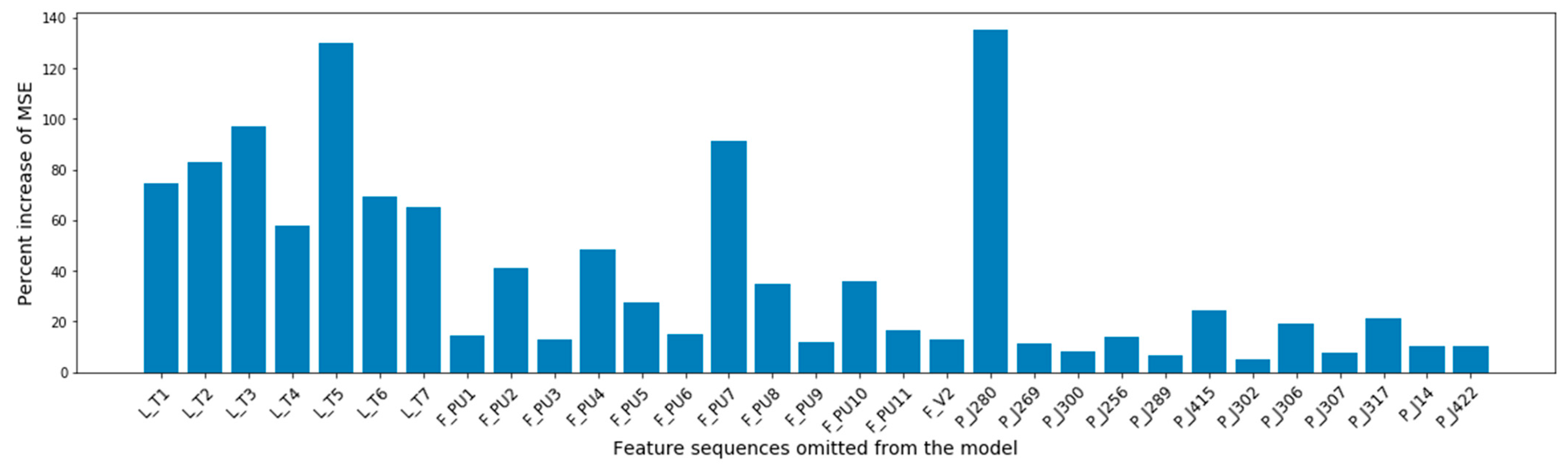
Figure 8 quantifies each feature’s contribution to the model’s forecasting accuracy. It shows the percent increase of the model’s overall MSE when a feature was omitted from the input of the model. The most influential features were the pressure at the junction that connected the reservoir with the water distribution network, and the water level at the network’s tanks. The model considered as more important the flow of the pumps that worked during the training set and tended to give less attention to pumps that were deactivated in the attack free set (PU3, PU5, PU6, PU9, and PU11).
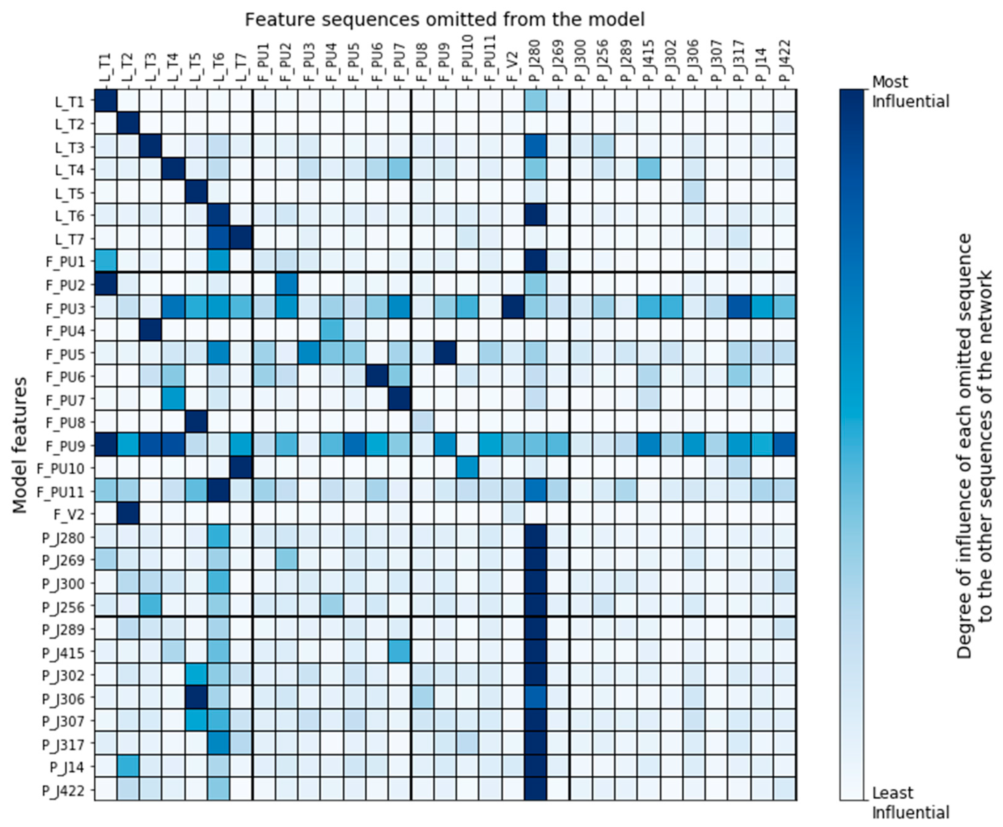
Figure 9 provides a node-level summary of the impact each feature sequence had on the other features of the network when it was omitted from the input. By examining which features were affected the most when removing a sequence, we could extract useful information regarding the interdependencies among the features as those were assigned by the deep learning model. For instance, we observed that the TGCN model mostly depended on what a tank’s water level was at previous timesteps to make a prediction about the tank’s current level. This means that tank levels were not influenced much by the other features of the network. On the other side, the working pumps of the network were influenced by tanks of the same DMA, meaning that the model could assign accurate relationships (based on the physical model) between the network’s components. However, the model, reasonably, failed to assign meaningful dependencies to the pumps that were closed during the entirety of the training set (PU3, PU5, PU6, PU9, and PU11). Another shortcoming of the model is that it failed to represent the actual interconnections of the network’s junctions. Instead, the junctions of the network were influenced almost exclusively by J280, which is the junction that connects the reservoir with the water distribution network.
It is interesting to notice that Tank 7 was strongly influenced by Tank 6. Perhaps this was why our algorithm disclosed Tank 6, instead of Tank 7, as the most likely under-attack-component during the attack scenario 13. Our ability to make this assumption highlights the importance of algorithm explainability. Having some insight into why algorithms behave as they should not, helps us take tailored-to-the-problem actions during development, such as improving the training data, refining specific features, and updating the model architecture.
4.5. Comparison with BATADAL Algorithms
The BATADAL contestants had at their disposal and to develop their algorithms. If we had participated in the competition, the model of our choice (out of the 20 trained models) would have been the one with the best performance (maximum score) in the holdout set, . Based on this criterion, we report the performance of our algorithm in Table 4. When compared with the algorithms that participated at BATADAL, TGCN ranks in the third position right after the algorithms proposed by Housh and Ohar [9] and Abokifa et al. [12]. Housh and Ohar proposed a model-based approach that requires a perfectly calibrated hydraulic model of the network. However, an accurate hydraulic model might be difficult to obtain in real-life settings, due to uncertainties in key model parameters (such as nodal demands, pipes roughness, etc.). Furthermore, it should be noted that Abokifa et al. proposed a multi-stage approach that operates using an alarm watch window procedure. The alarm watch window procedure might require a waiting period (starting from the moment the first anomaly is discovered) before an attack alarm is issued. This means that, as also acknowledged by Abokifa et al., the time to detection of the attacks () reported “does not reflect the practical time taken by the proposed algorithm when operated in real-time fashion” [12]. In comparison, TGCN does not require the use of a detailed physical model nor multi-stage techniques. As such, and given that the proposed algorithm is also explainable and can be implemented in real-time, we argue that it is an approach worthy of further exploration.
5. Discussion
We found that TGCN is a valuable tool for cyber–physical attack detection in water distribution systems. The proposed algorithm exhibited strong detection performance as it was capable of detecting all simulated attacks while issuing a small number of false positive instances. The small training variance and the fact that the algorithm retained its performance after changes made to the threshold tuning step indicates that the proposed algorithm possesses robust characteristics. Furthermore, for the majority of the benchmark attacks, the algorithm was capable of localizing the components directly targeted. Interestingly, the algorithm’s explainability properties made it feasible to also understand why the algorithm failed to detect directly targeted components for some attacks. We also conclude that the TGCN succeeded in learning how to represent the network since it assigned relationships between the network’s components that could be considered accurate based on the physical model.
The work also demonstrated that several performance metrics, which are commonly found in the literature, fall short when used as an objective function in the threshold tuning step. This was because the available metrics consider different observations as independent samples, failing to distinguish sequential from scattered false alarms or timely from delayed attack detection. As Taormina et al. noted [5], there is also a lack of metrics that consider the damage corresponding to the delayed detection of an attack. Hence, we also argue for the need of a set of novel metrics that are aligned with the cyber–physical attack detection objectives and account for the problem-specific characteristics of the SCADA datasets, as these would help accelerate the optimization process of threshold-based algorithms and provide a common framework for ranking different algorithms.
When compared with other algorithms developed for the BATADAL competition, the algorithm described in this work ranks among the best-performing ones. Despite not having the best performance [5], we argue that it presents a unique combination of advantages. Using the Mahalanobis distance as an anomaly score helps the practitioner select the anomaly detection parameters in a completely unsupervised way when a set with labeled attacks is unavailable. The algorithm is adaptable to real-time intrusion detection given that detection rules require only past or current data. Furthermore, it was capable of detecting and localizing attacks with a single model, without requiring multiple stages. The TGCN model is not only limited to anomaly detection but can also be used for tasks that require forecasting the system’s hydraulic state, such as real-time network optimization and management. Perhaps the most important characteristic of the algorithm is its explainability. This step towards “explainable AI” is important as it allows for the extraction of useful insights about how models work and contributes to trust-building by practitioners within water companies. This explainability could also be used to tailor algorithms using domain knowledge to detect vulnerabilities that would otherwise require extensive experiments and simulations when using purely black-box algorithms.
However, some limitations of the proposed algorithm should also be noted. First, it is not possible to calculate the Mahalanobis distance in higher dimensional datasets due to multicollinearity. Second, unlike the attack detection algorithm, the attack localization algorithm was not able to immediately identify the directly targeted component for all attack scenarios. Furthermore, given that the BATADAL datasets were generated using “fairly regular” demand patterns [5] and our algorithm is data-based, the question of whether it would retain its robustness when tested on real-life datasets remains unanswered. However, it could be argued that the fact that the model embeds the spatial information of its input features (in itself a form of prior knowledge), should help the algorithm retain (some of) its robustness compared to solely data-based algorithms. Finally, our algorithm’s robustness has not been tested against adversarial attacks. Although the benchmark attack scenarios contained manipulated SCADA readings, including attacks concealed by replay, further testing is required.
These remarks also point towards future research avenues. For example, the anomaly detection algorithm, although sufficient for the benchmark datasets, can be adapted to be efficient in higher dimensional datasets. The encouraging localization performance acts as a motivation to suggest the future development of a real-time attack localization-and-response algorithm combined with new performance metrics that consider the cost of not localizing an attack promptly. The robustness of the algorithm can be further validated by observing its performance in more realistic, stochastically generated datasets based on real-life network timeseries that also incorporate adversarial attacks.
6. Conclusions
We presented an online, one-stage, explainable algorithm for the detection of cyber–physical attacks in water distribution systems. The proposed algorithm’s uniqueness stems from its ability to simultaneously embed the temporal and spatial information of its input features. This was achieved by implementing temporal graph convolutional neural networks and the Mahalanobis distance. Based on the explainability and the good localization performance of the algorithm, we argue that the use of deep learning models that consider the graph structure of the water network is a promising research direction. It is hoped that this work will contribute to the further adoption and development of novel GNN algorithms in water infrastructure problems, and that it will motivate the adoption of common performance metrics that are better aligned to the challenge of cyber–physical attack detection in water distribution networks.
Author Contributions
Conceptualization, C.M.; methodology, L.T. and C.M.; software, L.T.; investigation, L.T. and C.M.; writing—original draft preparation, L.T.; writing—review and editing, L.T. and C.M.; visualization, L.T.; supervision, C.M. All authors have read and agreed to the published version of the manuscript.
Funding
This research received no external funding.
Institutional Review Board Statement
Not applicable.
Informed Consent Statement
Not applicable.
Data Availability Statement
Not applicable.
Conflicts of Interest
The authors declare no conflict of interest.
References
- Makropoulos, C.; Savić, D.A. Urban hydroinformatics: Past, present and future. Water 2019, 11, 1959. [Google Scholar] [CrossRef] [Green Version]
- Nikolopoulos, D.; Moraitis, G.; Bouziotas, D.; Lykou, A.; Karavokiros, G.; Makropoulos, C. Cyber-physical stress-testing platform for water distribution networks. J. Environ. Eng. 2020, 146, 04020061. [Google Scholar] [CrossRef]
- Hassanzadeh, A.; Rasekh, A.; Galelli, S.; Aghashahi, M.; Taormina, R.; Ostfeld, A.; Banks, M.K. A review of cybersecurity incidents in the water sector. J. Environ. Eng. 2020, 146, 03120003. [Google Scholar] [CrossRef] [Green Version]
- Tuptuk, N.; Hazell, P.; Watson, J.; Hailes, S. A systematic review of the state of cyber-security in water systems. Water 2021, 13, 81. [Google Scholar] [CrossRef]
- Taormina, R.; Galelli, S.; Tippenhauer, N.O.; Salomons, E.; Ostfeld, A.; Eliades, D.G.; Aghashahi, M.; Sundararajan, R.; Pourahmadi, M.; Banks, M.K.; et al. Battle of the attack detection algorithms: Disclosing cyber attacks on water distribution networks. J. Water Resour. Plan. Manag. 2018, 144, 04018048. [Google Scholar] [CrossRef] [Green Version]
- Kossieris, P.; Makropoulos, C. Exploring the statistical and distributional properties of residential water demand at fine time scales. Water 2018, 10, 1481. [Google Scholar] [CrossRef] [Green Version]
- Kossieris, P.; Tsoukalas, I.; Makropoulos, C.; Savic, D. Simulating marginal and dependence behaviour of water demand processes at any fine time scale. Water 2019, 11, 885. [Google Scholar] [CrossRef] [Green Version]
- Taormina, R.; Galelli, S.; Tippenhauer, N.O.; Salomons, E.; Ostfeld, A. Characterizing cyber-physical attacks on water distribution systems. J. Water Resour. Plan. Manag. 2017, 143, 04017009. [Google Scholar] [CrossRef]
- Housh, M.; Ohar, Z. Model-based approach for cyber-physical attack detection in water distribution systems. Water Res. 2018, 139, 132–143. [Google Scholar] [CrossRef] [PubMed]
- Brentan, B.M.; Campbell, T.E.; Gonzalez-Lima, F.; Manzi, D.; Ayala-Cabrera, D.; Herrera, M.; Montalvo, I.; Izquierdo, J.; Luvizotto, E. On-line cyber attack detection in water networks through state forecasting and control by pattern recognition. In Proceedings of the World Environmental and Water Resources Congress 2017, Sacramento, CA, USA, 21–25 May 2017; American Society of Civil Engineers: Reston, VA, USA, 2017; pp. 583–592. [Google Scholar]
- Pasha, M.F.K.; Kc, B.; Somasundaram, S.L. An approach to detect the cyber-physical attack on water distribution system. In Proceedings of the World Environmental and Water Resources Congress 2017, Sacramento, CA, USA, 21–25 May 2017; pp. 703–711. [Google Scholar]
- Abokifa, A.A.; Haddad, K.; Lo, C.; Biswas, P. Real-time identification of cyber-physical attacks on water distribution systems via machine learning–based anomaly detection techniques. J. Water Resour. Plan. Manag. 2019, 145, 04018089. [Google Scholar] [CrossRef]
- Ramotsoela, T.D.; Hancke, G.P.; Abu-Mahfouz, A.M. Behavioural intrusion detection in water distribution systems using neural networks. IEEE Access 2020, 8, 190403–190416. [Google Scholar] [CrossRef]
- Kadosh, N.; Frid, A.; Housh, M. Detecting cyber-physical attacks in water distribution systems: One-class classifier approach. J. Water Resour. Plan. Manag. 2020, 146, 04020060. [Google Scholar] [CrossRef]
- Ramotsoela, D.T.; Hancke, G.P.; Abu-Mahfouz, A.M. Attack detection in water distribution systems using machine learning. Hum. Cent. Comput. Inf. Sci. 2019, 9, 1–22. [Google Scholar] [CrossRef]
- Taormina, R.; Galelli, S. Deep-learning approach to the detection and localization of cyber-physical attacks on water distribution systems. J. Water Resour. Plan. Manag. 2018, 144, 04018065. [Google Scholar] [CrossRef]
- Chandy, S.E.; Rasekh, A.; Barker, Z.A.; Shafiee, M.E. Cyberattack detection using deep generative models with variational inference. J. Water Resour. Plan. Manag. 2019, 145, 04018093. [Google Scholar] [CrossRef] [Green Version]
- Quiñones-Grueiro, M.; Prieto-Moreno, A.; Verde, C.; Llanes-Santiago, O. Decision support system for cyber attack diagnosis in smart water networks. IFAC Pap. 2019, 51, 329–334. [Google Scholar] [CrossRef]
- Yu, B.; Yin, H.; Zhu, Z. Spatio-temporal graph convolutional networks: A deep learning framework for traffic forecasting. In Proceedings of the Twenty-Seventh International Joint Conference on Artificial Intelligence, Stockholm, Sweden, 13–19 July 2018; International Joint Conferences on Artificial Intelligence Organization: Seattle, WA, USA, 2018; pp. 3634–3640. [Google Scholar]
- Teh, T.; Auepanwiriyakul, C.; Harston, J.A.; Faisal, A.A. Generalised Structural CNNs (SCNNs) for Time Series Data with Arbitrary Graph Topology. arXiv 2018, arXiv:1803.05419v2. [Google Scholar]
- Covert, I.; Krishnan, B.; Najm, I.; Zhan, J.; Shore, M.; Hixson, J.; Po, M.J. Temporal Graph Convolutional Networks for Automatic Seizure Detection. arXiv 2019, arXiv:1905.01375v1. [Google Scholar]
- McLachlan, G.J. Mahalanobis distance. Resonance 1999, 4, 20–26. [Google Scholar] [CrossRef]
- Covert, I.; Lundberg, S.; Lee, S.-I. Explaining by removing: A unified framework for model explanation. arXiv 2020, arXiv:2011.14878v1. [Google Scholar]
Figure 1.
Different aggregation rules of the STC layer. Both rules begin by applying a 1D convolution along the temporal dimension and then: (a) Rule A aggregates features from the node’s neighborhood including the node itself, and (b) Rule B aggregates features from the node’s neighbors, and then combines these features with the node’s own features.

Figure 2.
Basic TGCN architecture for the time-series prediction task.

Figure 3.
Methodology outline: (a) Developing the TGCN model to predict current SCADA observations, (b) calibration of the attack detection scheme, (c) application process of the attack detection algorithm to new observations.
Figure 3.
Methodology outline: (a) Developing the TGCN model to predict current SCADA observations, (b) calibration of the attack detection scheme, (c) application process of the attack detection algorithm to new observations.

Figure 4.
(a) The network of C-Town, (b) the resulting condensed graph of the network, created based on the available measurements.
Figure 4.
(a) The network of C-Town, (b) the resulting condensed graph of the network, created based on the available measurements.

Figure 5.
Mahalanobis distance on the test set ( of BATADAL), before and after using a rolling mean window to avoid outliers.
Figure 5.
Mahalanobis distance on the test set ( of BATADAL), before and after using a rolling mean window to avoid outliers.

Figure 6.
Algorithm performance on the test dataset ( of BATADAL).

Figure 7.
Graphic performance of the algorithm on the holdout set (Dataset 2) using the same trained TGCN model, but different objective functions to fine-tune the attack detection threshold “” and rolling mean window length “”. Objective functions used: (a) score, (b) score, (c) BATADAL score.
Figure 7.
Graphic performance of the algorithm on the holdout set (Dataset 2) using the same trained TGCN model, but different objective functions to fine-tune the attack detection threshold “” and rolling mean window length “”. Objective functions used: (a) score, (b) score, (c) BATADAL score.

Figure 8.
Feature importance summarization based on the percent increase of the MSE after each feature’s omission.
Figure 8.
Feature importance summarization based on the percent increase of the MSE after each feature’s omission.

Figure 9.
Node-level summary of the impact each feature has on the other features of the network.


Table 1.
How different data availability scenarios (regarding the holdout set) affect the algorithm’s performance in the test dataset.
Table 1.
How different data availability scenarios (regarding the holdout set) affect the algorithm’s performance in the test dataset.
| Holdout Set | Objective Function | F1 Score | Precision | Recall | SCM | STTD | S |
|---|---|---|---|---|---|---|---|
| Dataset 2 (fully labeled) | max(S) | 0.813 ± 0.032 | 0.713 ± 0.05 | 0.948 ± 0.011 | 0.927 ± 0.011 | 0.933 ± 0.005 | 0.930 ± 0.005 |
| Dataset 2 (semi-labeled) | max(S) | 0.857 ± 0.021 | 0.800 ± 0.047 | 0.926 ± 0.018 | 0.934 ± 0.005 | 0.932 ± 0.008 | 0.933 ± 0.006 |
| Validation set | min(FP) | 0.873 ± 0.01 | 0.843 ± 0.022 | 0.906 ± 0.01 | 0.933 ± 0.004 | 0.93 ± 0.005 | 0.931 ± 0.004 |
Table 2.
Algorithm performance on the holdout set () using the same trained TGCN model, but different objective functions to fine-tune the attack detection threshold “” and rolling mean window length “”.
Table 2.
Algorithm performance on the holdout set () using the same trained TGCN model, but different objective functions to fine-tune the attack detection threshold “” and rolling mean window length “”.
| Algorithm * | (a) | (b) | (c) |
|---|---|---|---|
| Objective function | maximize(F1) | maximize(F2) | maximize(S) |
| Precision | 0.822 | 0.711 | 0.610 |
| Recall | 0.819 | 0.927 | 0.931 |
| F1 score | 0.821 | 0.805 | 0.737 |
| F2 score | 0.820 | 0.874 | 0.842 |
| SCM | 0.898 | 0.938 | 0.926 |
| STTD | 0.934 | 0.930 | 0.951 |
| S | 0.916 | 0.934 | 0.938 |
| TNR | 0.976 | 0.950 | 0.920 |
| TP | 403 | 456 | 458 |
| FP | 87 | 185 | 293 |
| TN | 3589 | 3491 | 3383 |
| FN | 89 | 36 | 34 |
* Each algorithm corresponds to the graphic performance of the algorithms showed in Figure 7.
Table 3.
Attack localization for the test set () of BATADAL. Components in bold correspond to the directly attacked components.
Table 3.
Attack localization for the test set () of BATADAL. Components in bold correspond to the directly attacked components.
| Attack Label | Attack Description | Features with the Highest Average MSE during the Attack (in a Descending Order) | |||
|---|---|---|---|---|---|
| Attack 8 | Alteration of L_T3 thresholds leading to underflow | L_T3 | P_J256 | ||
| Attack 9 | Alteration of L_T2 readings leading to overflow | L_T2 | P_J300 | P_J289 | P_J422 |
| Attack 10 | Activation of PU3 | S_PU3 | |||
| Attack 11 | Activation of PU3 | S_PU3 | |||
| Attack 12 | Alteration of L_T2 readings leading to overflow | L_T2 | P_J300 | P_J289 | |
| Attack 13 | Change the L_T7 thresholds | P_J302 | P_J307 | L_T6 | |
| Attack 14 | Alteration of T4 signal | P_J415 | L_T4 | ||
Table 4.
Comparison of TGCN with BATADAL algorithms.
| Number of Attacks Detected | S | STTD | SCM | TPR | TNR | |
|---|---|---|---|---|---|---|
| Housh and Ohar | 7 | 0.970 | 0.965 | 0.975 | 0.953 | 0.997 |
| Abokifa et al. | 7 | 0.949 | 0.958 | 0.940 | 0.921 | 0.959 |
| TGCN | 7 | 0.931 | 0.934 | 0.928 | 0.885 | 0.971 |
| Giacomoni et al. | 7 | 0.927 | 0.936 | 0.917 | 0.838 | 0.997 |
| Brentan et al. | 6 | 0.894 | 0.857 | 0.931 | 0.889 | 0.973 |
| Chandy et al. | 7 | 0.802 | 0.835 | 0.768 | 0.857 | 0.678 |
| Pasha et al. | 7 | 0.773 | 0.885 | 0.660 | 0.329 | 0.992 |
| Aghashahi et al. | 3 | 0.534 | 0.429 | 0.640 | 0.396 | 0.884 |
Publisher’s Note: MDPI stays neutral with regard to jurisdictional claims in published maps and institutional affiliations. |
© 2021 by the authors. Licensee MDPI, Basel, Switzerland. This article is an open access article distributed under the terms and conditions of the Creative Commons Attribution (CC BY) license (https://creativecommons.org/licenses/by/4.0/).
Share and Cite
MDPI and ACS Style
Tsiami, L.; Makropoulos, C. Cyber—Physical Attack Detection in Water Distribution Systems with Temporal Graph Convolutional Neural Networks. Water 2021, 13, 1247. https://doi.org/10.3390/w13091247
AMA Style
Tsiami L, Makropoulos C. Cyber—Physical Attack Detection in Water Distribution Systems with Temporal Graph Convolutional Neural Networks. Water. 2021; 13(9):1247. https://doi.org/10.3390/w13091247
Chicago/Turabian StyleTsiami, Lydia, and Christos Makropoulos. 2021. "Cyber—Physical Attack Detection in Water Distribution Systems with Temporal Graph Convolutional Neural Networks" Water 13, no. 9: 1247. https://doi.org/10.3390/w13091247
Note that from the first issue of 2016, this journal uses article numbers instead of page numbers. See further details here.