
A Moment-Based Chezy Formula for Bed Shear Stress in Varied Flow


1
Imam Mohammad Ibn Saud Islamic University, IMSIU, Riyadh 13318, Saudi Arabia
2
Irrigation and Hydraulics Department, Faculty of Engineering, Cairo University, Giza City 12613, Egypt
Water 2021, 13(9), 1254; https://doi.org/10.3390/w13091254
Submission received: 12 March 2021
/
Revised: 23 April 2021
/
Accepted: 26 April 2021
/
Published: 30 April 2021
(This article belongs to the Section Hydraulics and Hydrodynamics)
Abstract
:Despite its limitations, the Chezy bed shear stress formula is commonly used in depth-averaged flow numerical models as closure for estimating mutual tractive stresses with underneath boundaries. This paper proposes a novel moment-based formula that could be considered a revised version of the Chezy formula and can be used to estimate local variations of the bed shear stress under more complex and varied flow conditions with accelerating–decelerating flow fields. The formula depends on two velocity scales: the depth-averaged velocity, Uo, and a new moment-based velocity scale, u1. The new formula is calibrated using 10 experiments for flow over fixed bedforms, and the calibration coefficient is found to linearly correlate with h/Δ and h/zo ratios. The formula is also applied for the case of air flow across a negative step, jet water flow downstream a gate, and 2D water flow downstream an oblique negative step, and reasonably satisfactory agreement with the measured data is found. The new formula could be used in vertically averaged and moment models to disclose part of the information already lost by the vertical integration procedure.
1. Introduction
Knowing the spatial variation of the bed shear stress is essential for many river-engineering problems in which water–bed interactions affect the flow and its boundaries. Examples of these engineering problems include scour analysis [1] and the study of the evolution of bedforms in alluvial channels [2,3]. It also helps in understanding the variation of the bed resistance and consequently the water levels in natural rivers. In the previous bedform example, the location of the maximum bed shear stress is crucial for determining the growth/decay patterns of bed perturbations.
A number of bed shear stress formulae are found in the open channel literature for predicting the bed shear stress in water streams. The conventional Chezy formula (Equation (1)) is one of the oldest semi-empirical formulae that was first derived by the Irish pioneer engineer Chezy for uniform flow conditions in an open channel [4]. The formula had been proven to work also for non-uniform gradually varied flow (GVF) after replacing the bed slope by the energy slope. Both uniform and GVF Chezy forms could be re-written in velocity form instead of slope form, as given by Equation (3). Within this context, the Manning equation and the Colebrook equation (Equation (2)) could be looked at as bed roughness-refinement versions for the original Chezy equation [5].
In the boundary layer literature, a number of empirical formulae are also found, but they are generally functioning of the displacement thickness δ*, the momentum thickness θ, and the shape parameter H = δ*/θ. Each formula has its own conditions and assumptions. Examples of these formulae are the Ludwieg and Tillmann formulae [6]. Most of these boundary layer formulae were developed for the case of a high adverse pressure gradient with no streamline separation.
where τb is the bed shear stress, Uo is the depth-averaged water velocity, ρ is the water density, and C* is the dimensionless Chezy coefficient, which could be estimated using the Colebrook equation (Equation (2)) or the Manning equation (Equation (3)) as follows:
where h is the local water depth at a given location x, ks is the equivalent sand grain roughness height, n is Manning’s roughness coefficient, and g is the acceleration of gravity.
Depth-averaged flow models are widely used in planning and design of irrigation and drainage channels and streams, flood protection management, and flood hazard mapping and risk mitigation [7,8]. The majority of these models use the Chezy or Manning equation or what is alike as a constitutive law to predict energy losses due to friction. Although such models are highly successful, reliable, and convenient to use to predict the flow field parameters in terms of the local water depth and average water velocities in shallow water applications over a fixed bed, such models do not have the same success in movable-bed applications, partly because of our incomplete understanding of the sediment transport process [9] but mostly because of the averaging process adopted in the conventional depth-averaged models, which scarifies all the important near-bed velocity details and uses one single velocity scale, the depth-averaged velocity, (in each direction) to describe the local variation of bed shear stresses. As a result, depth-averaged models were not successful in studying the evolution of bedforms or in mapping the spatial variation of turbulence over a varying bed terrain [5].
To extend the capabilities of depth-averaged models, Steffler and Jin proposed in 1993 the vertically averaged and moment (VAM) technique, in which the degrees of freedom of the velocity profile increase from a constant mean value to a linear or parabolic distribution. In addition, the hydrostatic assumption is released and the non-hydrostatic effect is considered. To give closure for the new velocity scales and the non-hydrostatic pressure terms, the moment-of-momentum equations were solved, in addition to momentum equations [10]. Since that time, many research efforts have been conducted to use VAM models in different water flow applications, including flow simulation in bends [11,12], simulation of non-equilibrium sediment transport [13,14], stability of bedforms [15], dam break analysis [16], rapidly varied flow applications [17], and mixing due to secondary current [18].
Elgamal and Steffler proposed (without derivation) a 1D bed shear stress formula that is based on the moment-of-momentum approach [5]. The formula was used to investigate the spatial variation of bed shear stress over low-regime bedforms. The paper in-hand builds on the earlier research conducted by Elgamal and Steffler and contributes to further extending it to cover new applications not covered before.
In the method statement section (Section 2) of this paper, the moment-of-momentum concept is introduced and the analytical basis of the revised Chezy formula is presented and discussed. In Section 3, the results of the revised formula when applied to a number of 1D applications are discussed. The 1D applications include flow over a train of bedforms, flow downstream a negative step, and flow downstream a free gate with an existing free classic hydraulic jump. In addition, the 2D form of the formula is introduced and applied to the oblique negative-step problem. In Section 4, the proposed 1D formula is examined to check its capability to simulate the evolution of bedforms from an initially flatbed. Finally, conclusions and recommendations are stated.
2. Method Statement
2.1. The Moment-of-Momentum Concept
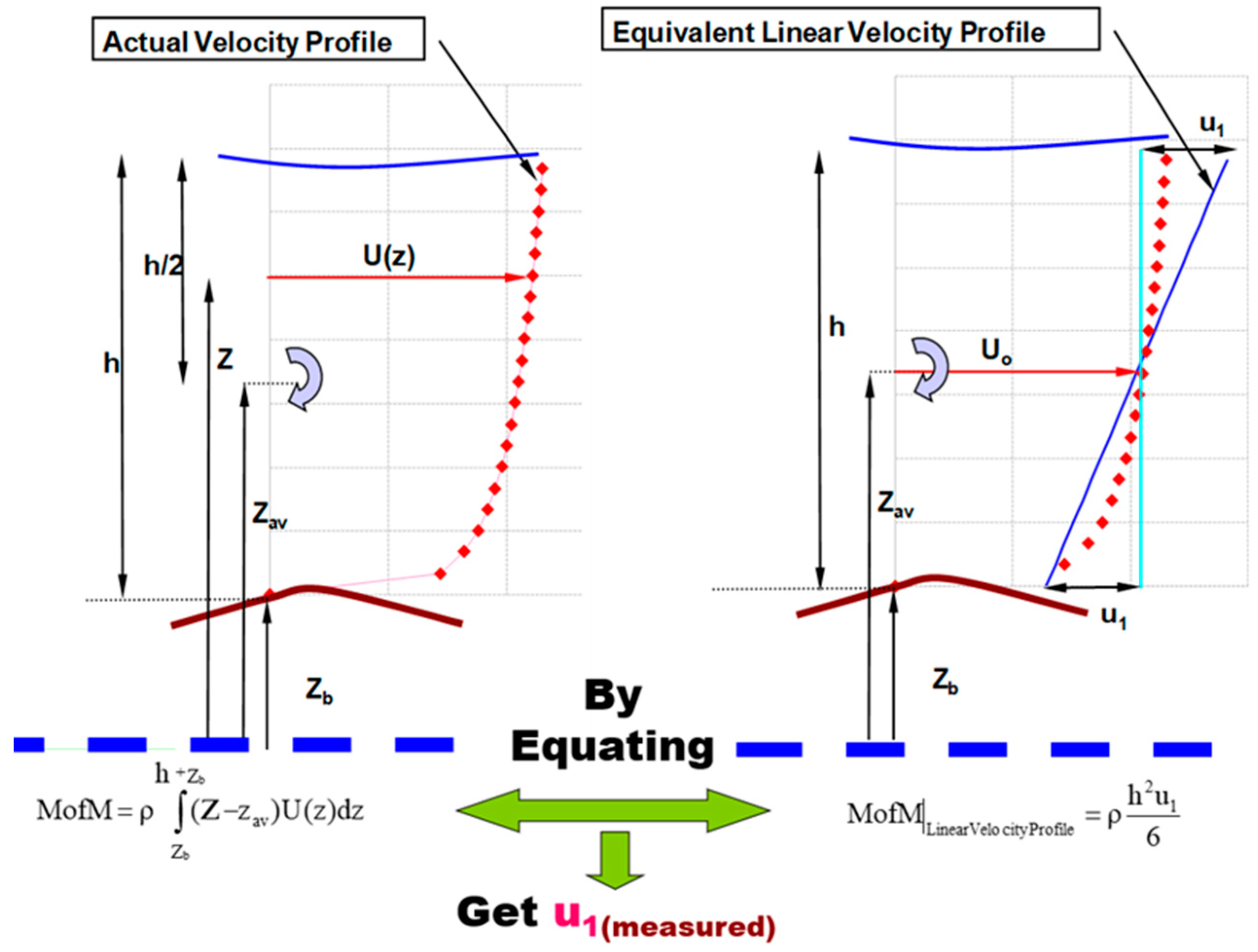
In conventional depth-averaged flow models, almost all the degrees of freedom of the velocity profile are suppressed by using a vertically constant velocity profile in place of the real one, whereas in the moment approach, the degrees of freedom of the model’s vertical distribution of the streamwise velocity are increased. Each velocity profile is virtually converted to an equivalent linear velocity profile having the same discharge intensity and the same moment of momentum (MofM) around the mid-point of the water depth (Figure 1).
Following this idea, a new integral velocity scale, u1, is defined and calculated using Equation (4). A special case of Equation (4) is Equation (5), which gives the value of u1 in the case of uniform flow where the velocity profile could be assumed to be a logarithmic relation.
where z is the vertical coordinate normal to the flow, u(z) is the downstream velocity at level z above the datum, zb is the local bed level, h is the local water depth at a given location x, u1log is the moment velocity scale in the case of having a logarithmic velocity profile, α is a dimensionless coefficient that gives the ratio between u1log and the corresponding depth-averaged velocity in the case of a logarithmic velocity profile, and κ is the von Karman constant.
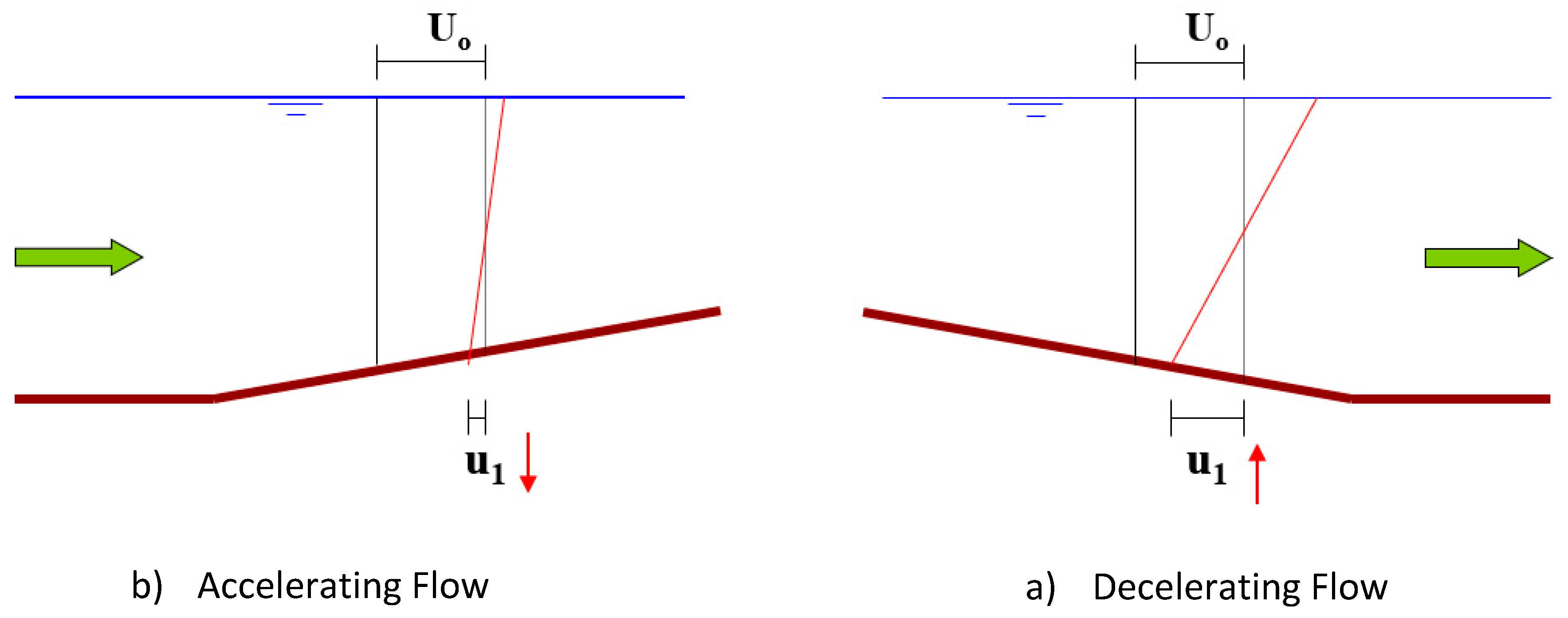
It should be mentioned that the value of u1 is the moment velocity scale, and it is a measure of the uniformity of the shape of the velocity profile. When the flow is accelerating, the shape of the velocity becomes more uniform, and consequently, u1 becomes small compared to its corresponding value in the case of decelerating flow (Figure 2). In contrast, a high positive value of the ratio u1/Uo means that the local velocity profile deviates considerably from the corresponding logarithmic profile. As the apparent bed velocity becomes smaller, this could be considered a sign of flow separation.
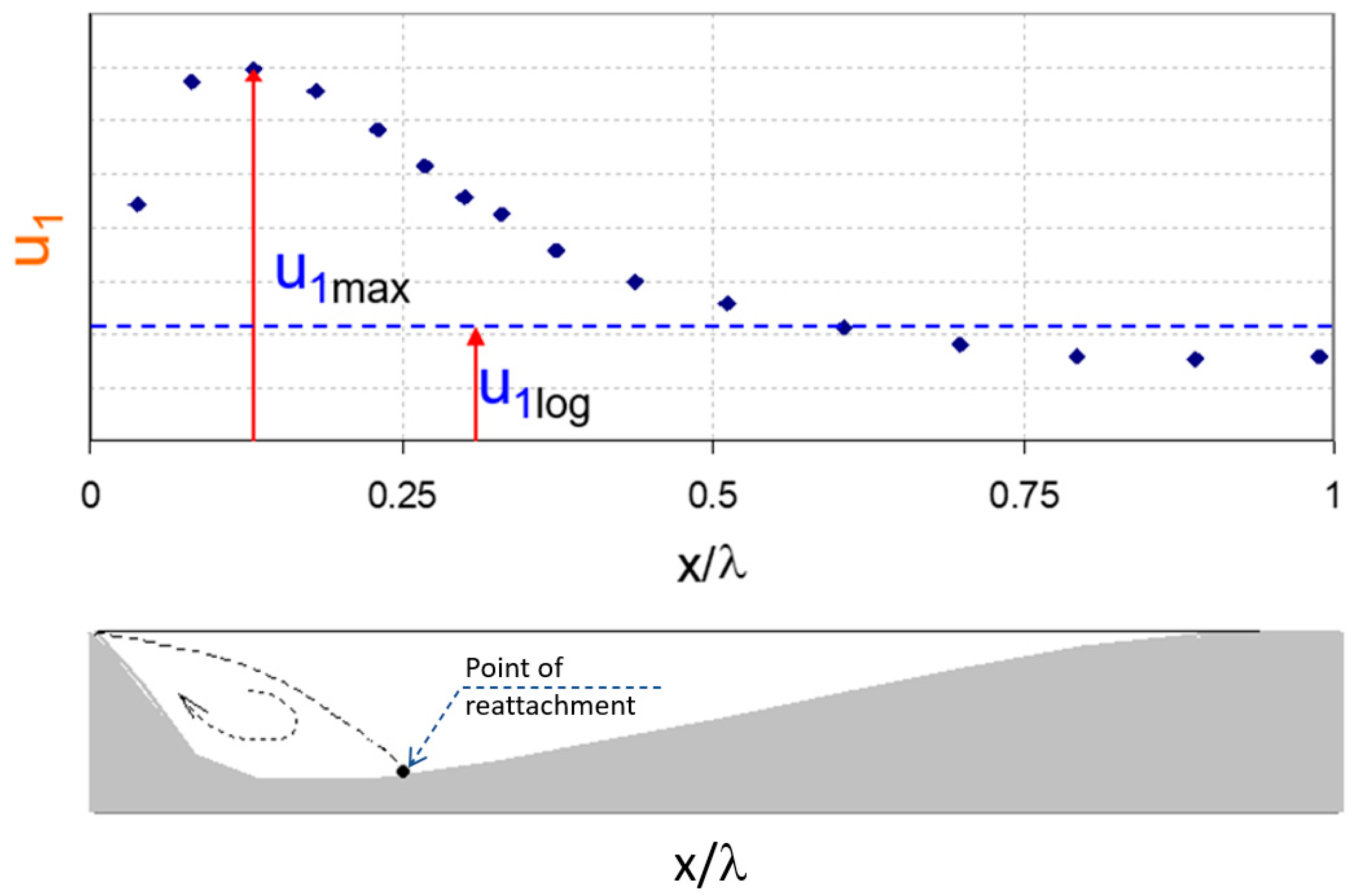
Figure 3 shows a typical spatial variation of u1 over one wavelength of a bedform. It is noted that u1 is spatially a continuous function and its value starts to increase downstream of the crest until it reaches a maximum value within the separation zone. After this point, u1 decreases downstream until it reaches its minimum near or over the crest. Figure 3 also compares the spatial variation of u1 as a function of distance x, and the corresponding value in the case of uniform flow over a flat bed, u1log, where the velocity profile can be assumed to be a logarithmic profile.
It should be noted that the value of u1 could be positive, similar to the case presented in Figure 3, or it could be negative, as the case of the underneath jet flow downstream a gate (more emphasis will be given to this point later).
2.2. Main Assumptions
The study in hand considers the following main assumptions:
- The flow is shallow, and the channel stream width is generally wide.
- The non-hydrostatic effects are negligible or disregarded.
- The fluid is Newtonian.
- The flow is turbulent.
2.3. New Moment Bed Shear Stress Formula
The bed shear stress can be calculated following an eddy viscosity concept as
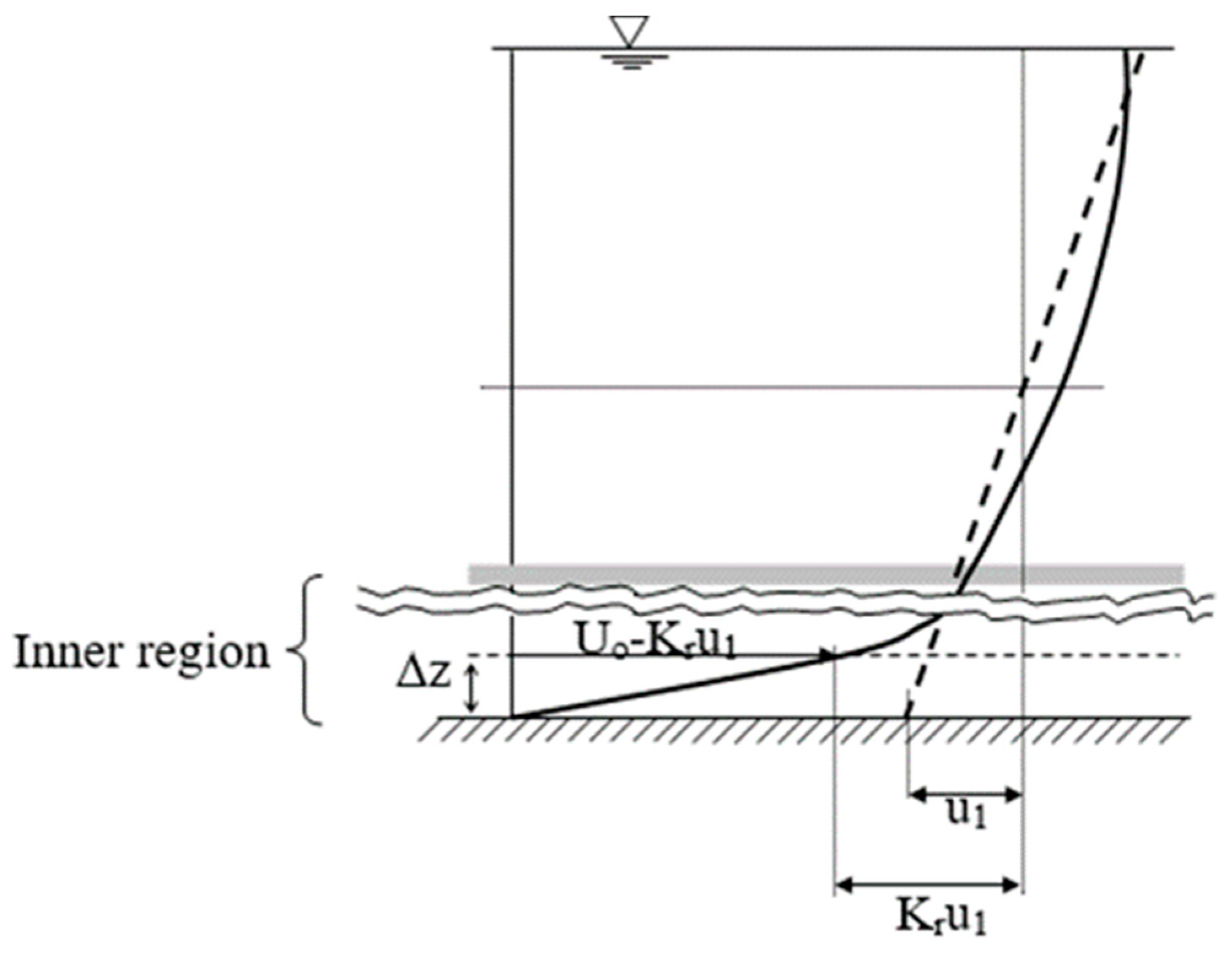
where νt is the eddy viscosity coefficient. Figure 4 shows that the velocity gradient close to the bed is generally larger than the average gradient of the equivalent linear velocity profile. Therefore, a new coefficient called Kr is introduced; the role of the coefficient Kr is to give a more reasonable estimation of the near-bed velocity. Thus, the vertical gradient of the water velocity near the bed can be approximated as
The near-bed eddy viscosity can be approximated following [19] as
where v and are the turbulence velocity and length scales, respectively; fo is a constant; and Δz is the numerical discretization for the vertical dimension. From Equations (6)–(10), the following local-bed shear stress formula is obtained:
where C2 can be written as C2 = . Equation (11) relates the bed shear stress to two velocity scales: the integral moment-based velocity scale u1, in addition to the depth-averaged velocity scale Uo. In addition, Equation (11) contains two dimensionless coefficients, C2 and Kr. C2 is the revised Chezy dimensionless coefficient, and it can be determined using Equation (12), which maintains the capability of the new formula to be reduced to the original Chezy formula in the case of uniform flow.
2.4. Calibration of the New Moment Bed Shear Stress Formula
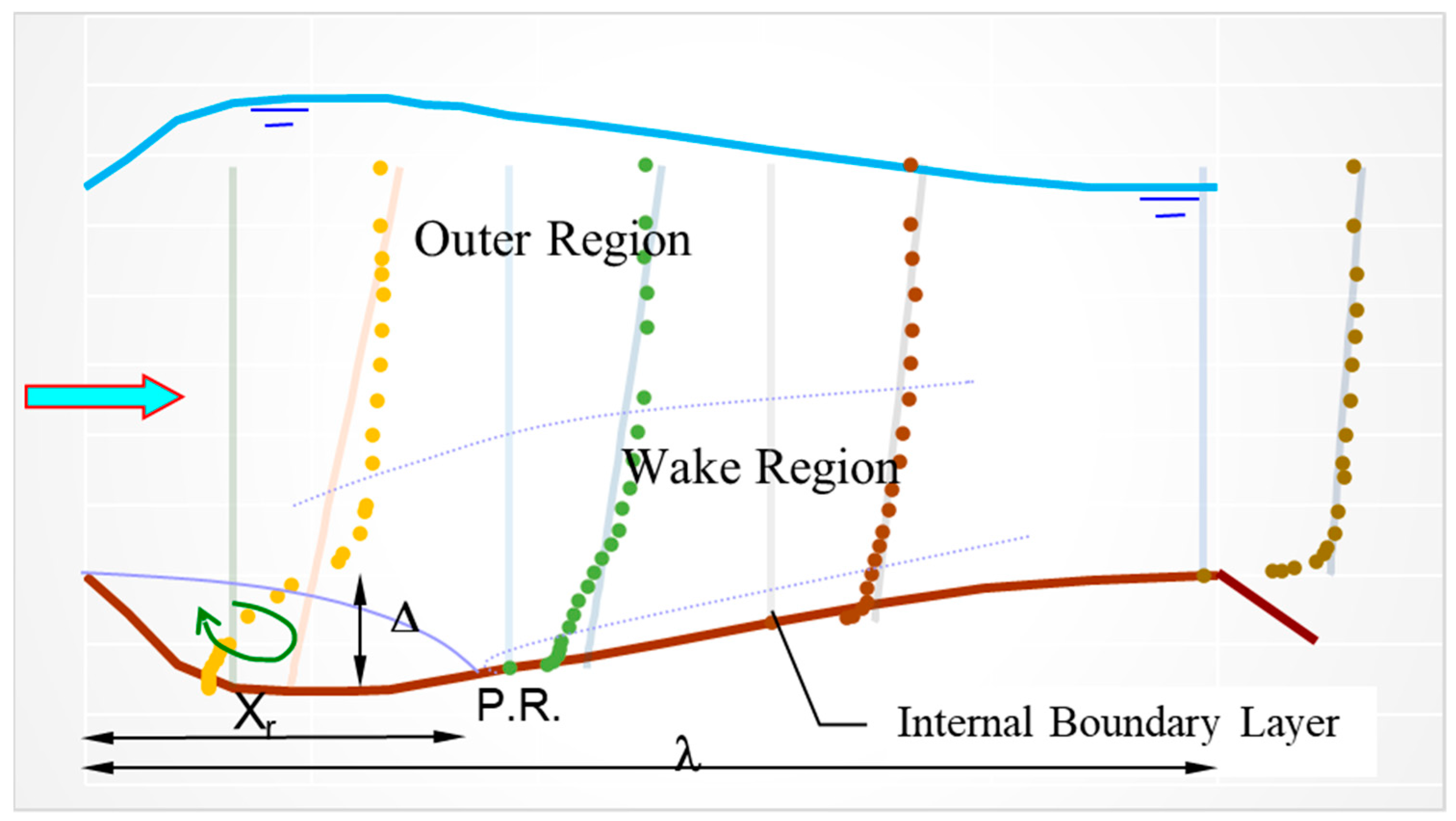
The new formula (Equation (11)) includes a new calibration coefficient Kr. To determine the range of this coefficient, the formula could be calibrated by using a set of lab experiments. For this purpose, a number of lab experiments (previously reported in the literature by other researchers) for the flow over a train of bedforms were selected. The reasons behind specifically selecting this type of experiment, flow over bedforms, are twofold: First, the flow structure is quite complicated and it contains both decelerating and accelerating flow zones. Second, separation might exist in the decelerating zone, causing a mismatch between the directions of the near-bed velocities and the depth-averaged velocities (Figure 5).
Table 1 lists the flow parameters and bed geometry of the selected experiments to be used in this study. Most of these laboratory experiments are for transitional roughness surfaces where the dimensionless sand grain roughness lies between 5 and 70. The dimensionless Chezy coefficient ranges from 15 to 20. The steepness ratio ranges from 1/10 to 1/20, and the crest-height-to-water-depth ratios range from 0.07 to 0.3, with the Froude number varying from 0.1 to 0.32 and a channel width (b) that varies from 0.08 to 1.5 m.
The calibration coefficient, Kr, can be determined by two different ways. The first is by setting the local bed shear stress to zero at the location of the point of reattachment. This condition can give a relation for Kr as
Kr = Uo/u1 (at the point of reattachment)
The second approach is by best-fitting Equation (11) to the experimental data.
Considering a periodic steady-state flow over a train of bedforms, the velocity ratio (Uo/u1) at the point of reattachment (i.e., Kr) could be written as
where ν is the kinematic viscosity; g is the acceleration of gravity; Δ and λ are the bedform height and wavelength, respectively; and zo is the roughness parameter thickness (zo = ks/30 + 0.11ν/u *).
Using dimensional reasoning, the following dimensionless parameters are obtained:
where Rn and Fn are the Reynolds and the Froude number, respectively. Since Fn 2 << 1, the effect of water surface waves and hence gravity effects can be neglected. In addition, for large values of Rn, viscous effects can be neglected.
The influence of the above parameters was examined by using the available experimental data. It is noted that the ratio λ/Δ has a minor effect on Kr. Thus, Equation (16) can be reduced to
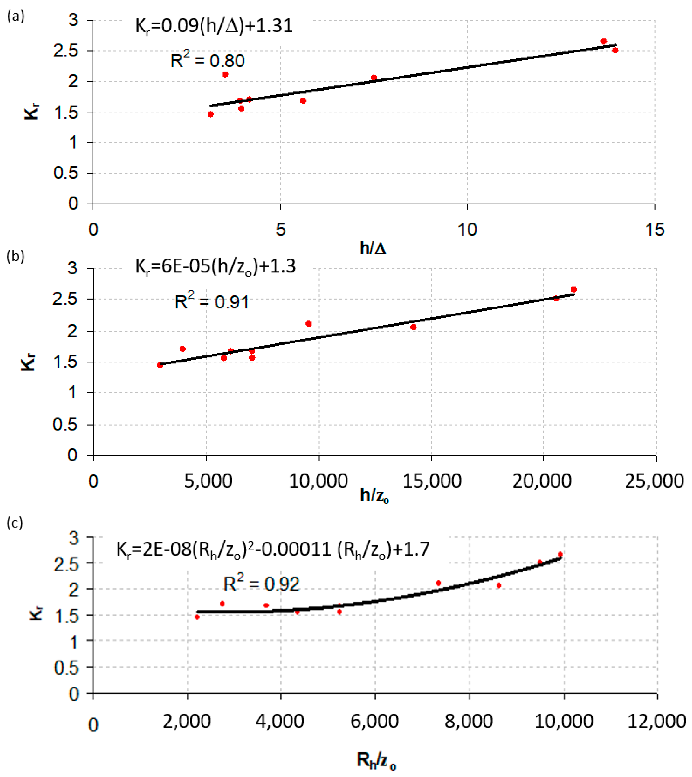
The effect of h/Δ on the calibration coefficient, Kr, is presented in Figure 6a. It is shown that as h/Δ gets bigger, Kr increases. This can be explained as follows: For a given value of the water depth and the flow intensity, as Δ increases, the thickness of the wake region gets bigger, causing u1 and the ratio Uo/u1 at the point of reattachment (i.e., Kr) to decrease. The correlation between Kr and h/Δ is given as
Kr = 1.31 + 0.09h/Δ r2 = 0.8
The influence of the surface roughness of the bedform is presented in Figure 6b. It is shown that (for a given value of the water depth and the flow intensity) as the surface roughness increases, the near-bed velocity becomes smaller, resulting in a larger value of u1 (i.e., a smaller value of Uo/u1 or Kr). Thus, Kr can be related to the depth-to-roughness ratio, h/zo, via a linear correlation, Equation (19).
Kr = 1.3 + 6.0 × 10⁻⁵ h/zo r2 = 0.91
In Equation (19), the surface of the bedforms in Raudkivi’s experiment [22] was assumed to be covered with a 0.2 mm sand layer (following the same assumption as in [26,27].
If the surface roughness in Raudkivi’s experiment is assumed to be smooth, then the Kr−h/zo relation could be given as
Kr = 1.28 + 5.7 × 10⁻⁵ h/zo r2 = 0.81
Equations (18)–(20) can be used as guidelines to obtain an estimate of the expected range of the calibration coefficient, Kr.
It should also be mentioned that some of the experiments were carried out in narrow channels and the ratio of the flume width to the water depth (b/h) ranged from 0.6 to 6. Accordingly, a side-wall correction might be required. One simple way to consider the side-wall effect is to use the hydraulic radius, Rh, instead of the water depth. In this case, the Kr–Rh/zo relation can be given as (Figure 6c)
where Rh is the hydraulic radius (Rh = bh/(b + 2h)) and b is the flume width.
Kr = 1.7 − 1.12 × 10⁻⁴ Rh/zo + 2.02 × 10⁻⁸ (Rh/zo)2 r2 = 0.92,
It should be emphasized that the paper in hand gives some formulae for predicting the calibration coefficient, Kr; however, such formulae should be used with caution, and more effort is required to be conducted to study the dependence of the coefficient Kr. For this regard, more data sets are required to be used that cover a wide spectrum of flow variation.
2.5. Revised 2D Horizontal Chezy Formula for Bed Shear Stress
It is quite interesting to investigate the performance of the new formula in 2D problems. The proposed 1D bed shear stress model can be extended to 2D applications for cases of induced non-uniform flow as a result of varying bed topography. By analogy with the existing 2D Chezy resistance formula, Equations (22) and (23) might be proposed as bed shear stress predictors for the x and y directions, respectively.
where τbx is the local bed shear stress component along the flow x direction, τby is the local bed shear stress component along the lateral y direction, Vo is the depth-averaged velocity in the y direction, and v1 is the integral moment velocity scale in the y direction (lateral direction) corresponding to u1 in the x direction (downstream direction).
In the next section, the 1D and 2D versions of the revised Chezy formula are applied to a number of applications to examine the revised form relevance.
3. Discussion and Results
3.1. 1D Applications
3.1.1. Low-Flow Regime over Bedforms
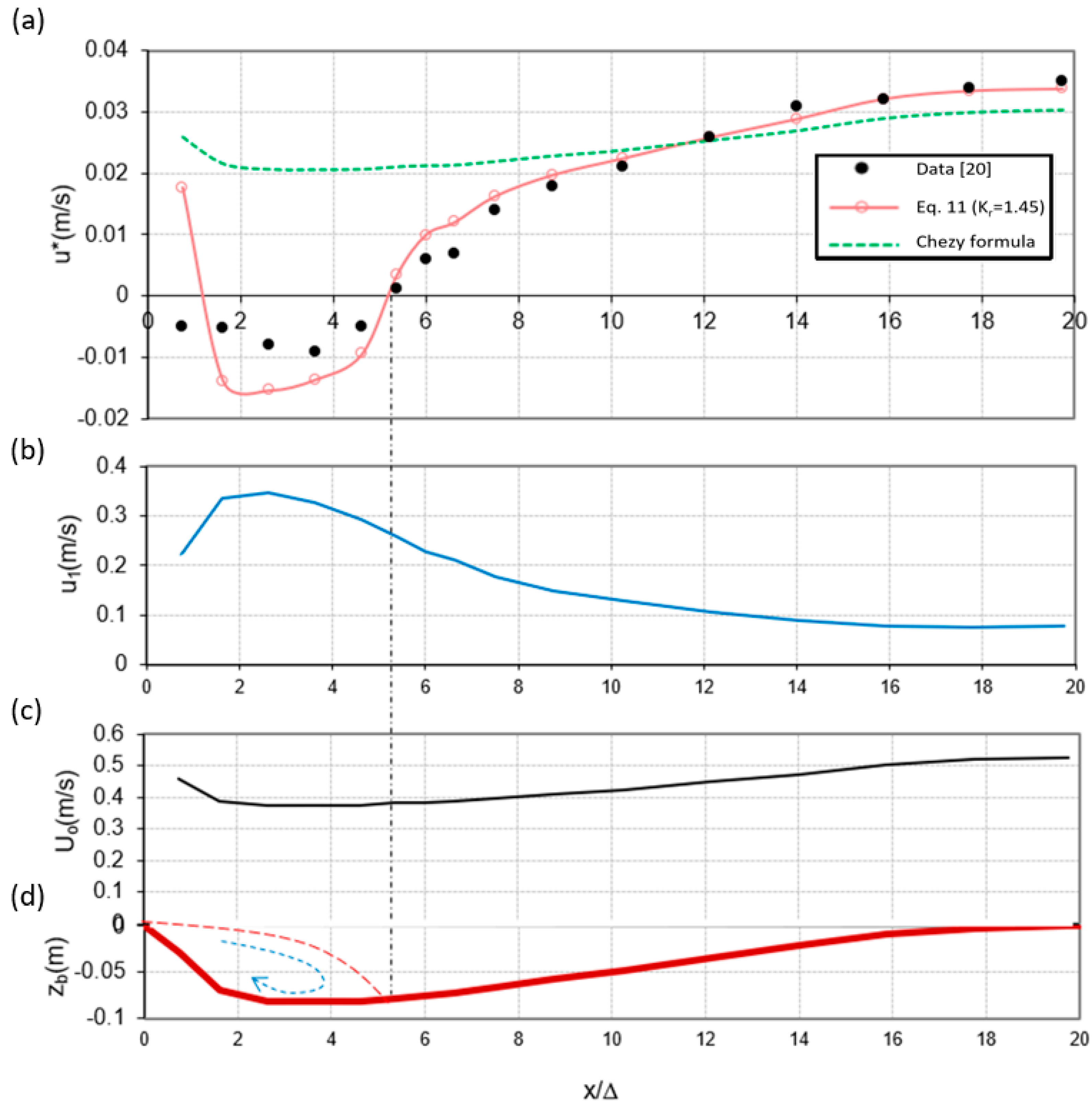
Figure 7a–c show the spatial variation of the bed shear velocity, u1 and Uo velocity fields for the case of low-regime shallow water flow over a train of fixed bedforms (Run 1 in Table 1). Figure 7d shows the typical geometry of one bedform with the circulation zone and the point of reattachment. The measurements (solid black circles) of the bed shear velocity were conducted by Van Mierlo and de Ruiter [20] and are compared by the conventional Chezy formula (Equation (1)) and the new moment formula (Equation (11)).
The spatial variations of the u1 and Uo velocities (shown in Figure 7b,c) are derived from the velocity profile measurements by numerically integrating the velocity profile measurements throughout the full water depth to get the depth-averaged velocity, Uo, and the new moment velocity, u1, with the help of Equation (4). A simple Matlab script was coded for this purpose to automate Uo and u1 calculations.
The results of the bed shear velocity show that the new moment formula (Equation (11)) generally captures the spatial variations in the bed shear velocity reasonably well, especially within the circulation zone, contrary to the conventional Chezy formula (Equation (1)).
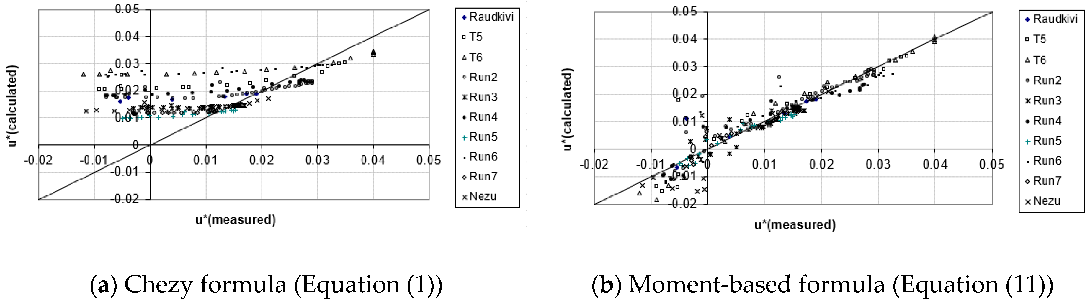
Figure 8a and Figure 8b present a comparison between the measured bed shear velocities and the predictions using Equations (1) and (11), respectively, for all the bedform experiments listed in Table 1. The new formula generally gives a good match with the measurements after the point of reattachment. Within the separation zone, the formula, on the one hand, seems to correctly produce the direction of the bed shear velocity but, on the other hand, generally over-predicts the shear velocity within the separation zone.
Given the uncertainties of the bed shear velocity measurements within the eddy zone, one can say that the general performance of Equation (11) is reasonable.
3.1.2. Air Flow over a Negative Step
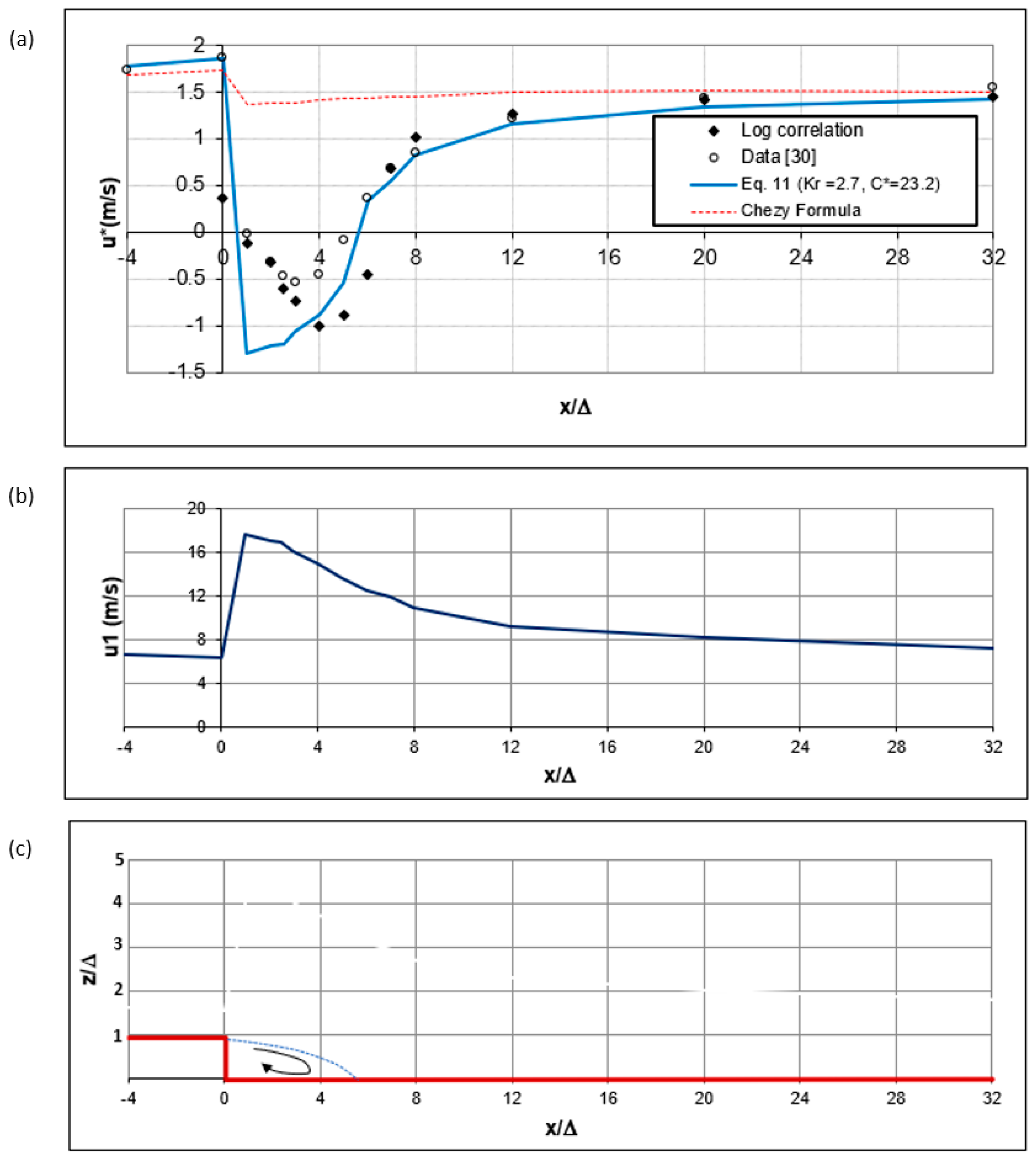
It is also of interest to test the formula for the backward (negative)-step problem (Figure 9c). This might be considered a special case of bedform with a wavelength of infinity [28]. Raudkivi [21] also found a strong similarity between the flow conditions downstream of the crest of a ripple and those of a negative step. This problem has a practical interest on its own, as the backward-facing step is often observed downstream of some hydraulic structures such as water gates and weirs [29]. Accordingly, the new formula has been used to predict the local bed shear stress of airflow over a negative backward step in a wind tunnel. The details of this experiment could be found in [30].
The spatial variations of the u1 velocities (shown in Figure 9b) are derived from the velocity profile measurements by numerically integrating the velocity profile measurements with the help of Equation (4). It is noted that u1 gets its maximum value just downstream of the step brink within the separation zone and then it starts to decrease downstream.
Skin friction was measured via an oil-flow laser interferometer. To use Equation (11) to predict u*, an equivalent free surface was assumed halfway of the tunnel height. Figure 9a presents the predictions of u* using the Chezy equation and Equation (11) and how they match with the measurements. It is noted that the difference between the measured bed shear velocity with the oil-laser interferometer and the predictions using the log law assumption is not significant, especially after the point of reattachment.
While the new formula is not able to accurately predict the shear velocity within the separation zone, it is capable of capturing the general spatial variations of the shear velocity reasonably well.
Figure 7a shows that the Chezy equation slightly underestimates the bed shear velocity near and over the crest. This might be explained by the effect of the topographically induced acceleration [31]. Downstream of the point of reattachment, the upward slope of the front side of the bedform helps in gradually converting the non-uniform velocity profile, caused by separation, to a uniform velocity distribution. In other words, the topographically induced acceleration helps in decreasing the value of u1 as the flow moves downstream. If the wavelength of the bedform is long enough, u1 might become less than u1log, which means that the shape of the velocity profile is more uniform than the corresponding logarithmic profile. Therefore, the Chezy equation underestimates the bed shear stress. In the case of the negative-step experiment, there is no upward slope and the effect of the topographically induced acceleration is not present. Therefore, the Chezy equation does not under-predict the maximum bed shear velocity near the downstream end, as shown in Figure 9a.
3.1.3. Water Jet Flow Downstream a Free Gate
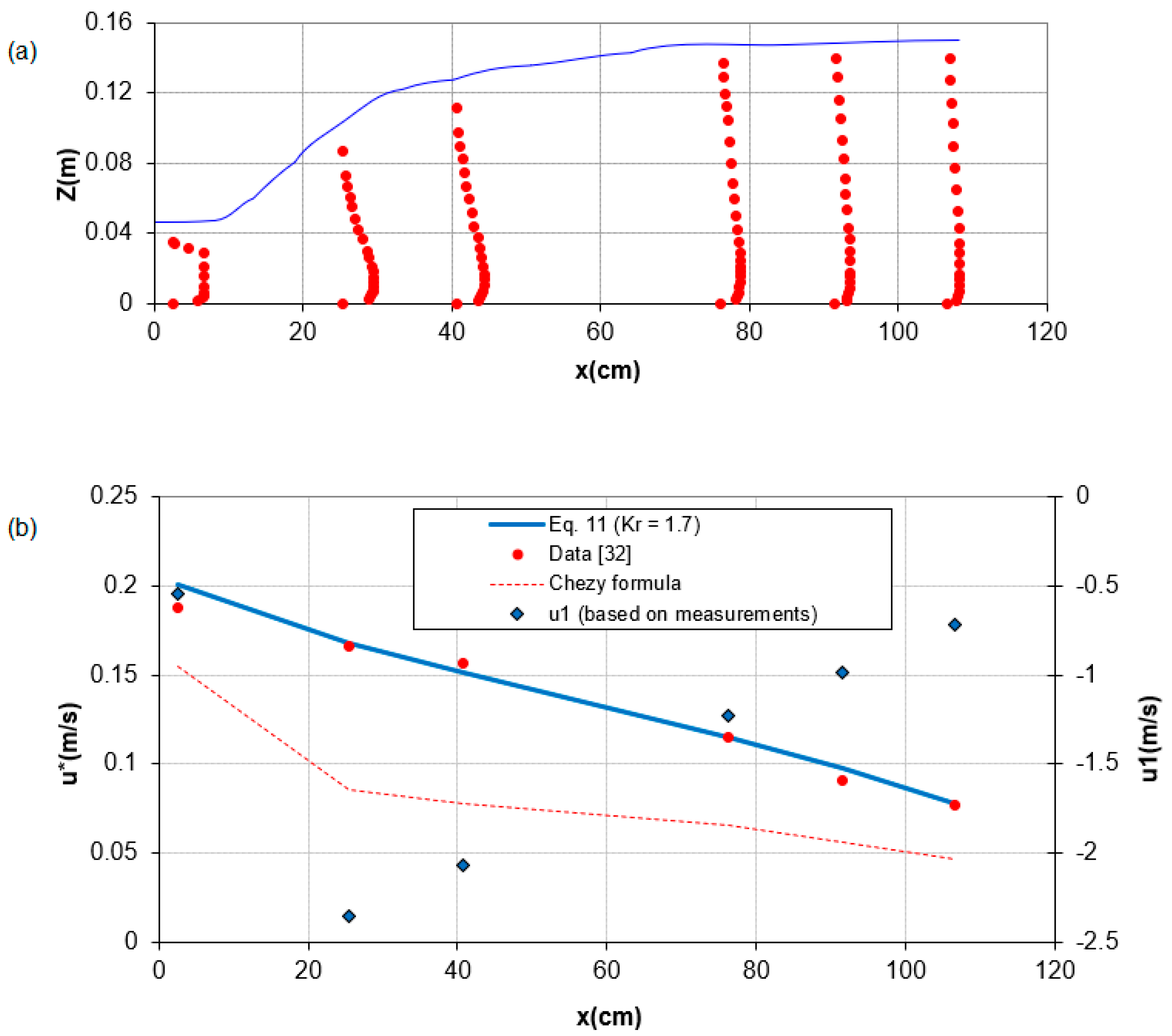
The new formula is also examined for predicting the spatial variation of the shear velocity for a near-bed water jet that is emerging and expanding downstream a free gate and forming a spatial hydraulic jump (S-jump). The full details of the laboratory experiment are found in [32]. Figure 10a shows the measured velocity profiles and water surface downstream of the jet outlet.
Figure 10b shows a double-Y plot that presents the spatial variations of u1 (in the right y axis) and the bed shear velocity (in the left y axis) downstream of the jet outlet.
Due to the closeness of the jet from the bed, the near-bed velocity is quite high compared to the depth-averaged velocity, causing u1 to have negative values, with the highest negative value just downstream from the jet outlet.
The new bed shear stress formula was able to capture the spatial variations of the bed shear velocity reasonably well and much better than the conventional Chezy formula.
3.2. 2D Application
It is quite interesting to investigate the performance of the new formula in 2D problems. Based on Equations (22) and (23), the angle of the bed shear stress with respect to the flow direction can be calculated as follows:
It should be mentioned that Equation (24) could be reduced to tan αb = Vo/Uo in the case of the conventional Chezy resistance formula.
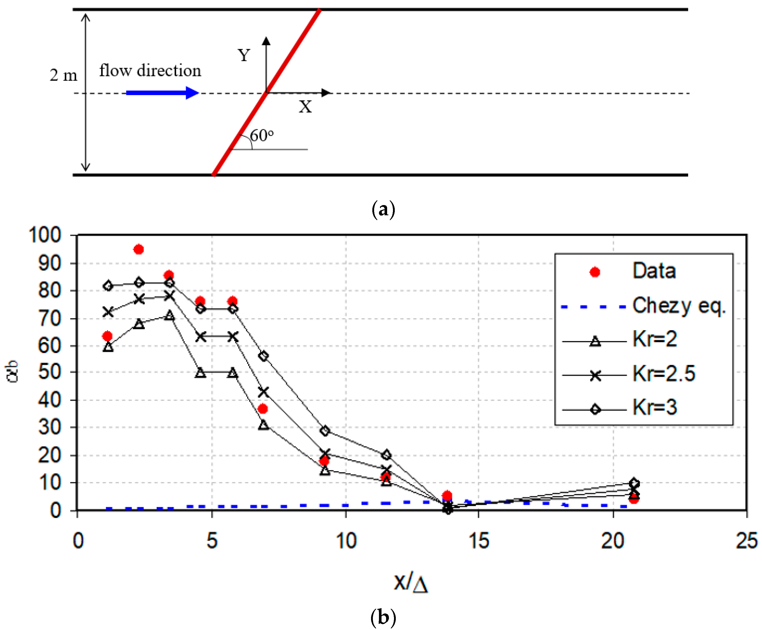
To test the behavior of the proposed formula, an oblique backward step experiment was selected for this purpose. Hasbo [33] carried out an experimental investigation of water flow over an oblique backward-facing step. The height of the step is 0.055 m and the angle is 60° with the direction of the flow (Figure 11). The flow was adjusted to a Froude number of 0.17, and the downstream water depth was kept at 0.4 m. The mean flow and turbulence intensities were measured using a two-component laser doppler anemometer. Because of the existence of the oblique step, the flow separates just downstream of the oblique crest, forming a corkscrew eddy within the separation zone. In addition, the near-bed flow streamlines are twisted, producing a skewed 3D boundary layer up to a distance of about 20 times the step height downstream of the crest.
To estimate the calibration coefficient, Kr, Equations (18)–(21) were used, which gave values ranging between 2.0 and 3.6. Figure 11b shows the variation of the direction of the near-bed velocity obtained from LDA measurements downstream of the oblique step through the centerline of the flume [32]. Within the separation zone, the direction of the near-bed velocity is significantly different from the direction of the downstream flow by an angle of 60° or more. Figure 11b presents the predictions of the Chezy equation as well as the new formula (Equation (11)) for values of Kr ranging from 2 to 3. Using Equation (11) to get the near-bed velocity direction implicitly reveals an assumption that claims that the near-bed velocity direction is the same as the angle of the resultant bed shear stress. This assumption was found reasonable by Hasbo (1995), who found good agreement between the directions of the measured near-bed velocities via LDA and the directions obtained by the behavior of tufts attached to the bed.
In reference to Figure 11b, although none of the models were able to precisely predict the actual values of the angle in the separation zone, the new formula generally showed good agreement compared to the conventional Chezy formula.
4. Conclusions and Challenges
A new local bed shear stress formula is proposed that can be used for cases of flow over a variable bed terrain and non-uniform flow conditions with accelerating–decelerating flow. The new formula describes the local bed shear stress using a new integral velocity, u1, in addition to the mean velocity. The new formula is calibrated using 10 laboratory experiments reported in the literature. The calibration coefficient represents a near-bed velocity correction and is found to correlate with h/Δ and h/zo ratios. The new bed stress formula might be considered a modified version of the Chézy resistance equation for non-uniform flow cases and could be used in depth-averaged flow models. The moment-of-momentum equation (VAM model) provides a means to calculate the additional integral velocity, u1.
A 2D version of the new formula is also proposed and used to predict the direction of the near-bed velocity downstream of an oblique negative step. The agreement with the measured data is reasonably satisfactory. More effort should be made in this part to test the proposed formula using other applications where the flow becomes non-uniform because of the non-uniformity of the bed.
This study will help in extending the validity of the depth-averaged flow models to be used in cases where non-uniformity significantly affects velocity distributions. An example of these cases is the flow over a variable terrain, including alluvial bedforms, which means saving time and storage space, compared to three-dimensional models.
It is also important to investigate the capability of the new bed shear stress formula to simulate bedform evolution. For this purpose, a linear stability analysis should be conducted first, followed by an evolution study of bedforms from initially flatbed conditions. The findings of the last said investigation will be discussed in a future paper.
Funding
This work was supported by a grant from the Natural Sciences and Engineering Research Council of Canada.
Institutional Review Board Statement
Not applicable.
Informed Consent Statement
Not applicable.
Data Availability Statement
Data are available on request from the authors.
Acknowledgments
The authors would like to thank professor Peter Steffler for his continuous support and valuable discussion during the study. The authors would also like to acknowledge the help of J. M. Nelson, S. R. Mclean, S. R. Wolfe, D. A. Lyn, I. Nezu, A. Kadota, S. Jovic, and D. M. Driver for providing their digital measurements and data.
Conflicts of Interest
The authors declare no conflict of interest.
Abbreviations
| b | channel/flume bed width |
| C* | original dimensionless Chezy coefficient |
| C2 | revised dimensionless Chezy coefficient (refer to Equation (12)) |
| Fn | dimensionless Froude number |
| fo | a constant (refer to Equation (10)) |
| g | acceleration of gravity |
| h | local water depth at distance x |
| Kr | dimensionless calibration coefficient with a value ranging from about 1.45 to 2.7 |
| ks | equivalent sand grain roughness height |
| n | Manning’s roughness coefficient |
| Rh | hydraulic radius (flow area/witted perimeter) |
| Rn | dimensionless Reynolds number |
| Uo | depth-averaged water velocity along the flow x direction |
| u1 | moment velocity scale along the flow x direction (refer to Figure 1) |
| u1max | maximum value of u1 (refer to Figure 3) |
| u1log | moment velocity scale in the case of logarithmic velocity profile |
| u(z) | downstream velocity at level z above the datum |
| u* | local bed shear velocity |
| Vo | depth-averaged velocity along the lateral y direction |
| v1 | moment velocity scale along the lateral y direction (refer to Equation (23)) |
| x | horizontal coordinate in the flow direction |
| Xr | location of the point of reattachment from the crest of the bedform |
| z | vertical coordinate normal to the flow and measured from a given arbitrary horizontal datum |
| zav | vertical distance from a given arbitrary horizontal datum up to the mid water depth |
| zb | local bed level |
| Δz | numerical discretization in the z direction |
| MofM | moment of momentum (refer to Figure 1) |
| VAM | vertically averaged and moment model |
| α | ratio between u1log and Uo (refer to Equation (5)) |
| αb | angle of the bed shear stress with respect to the flow direction (refer to Equation (24)) |
| Δ | bedform height (refer to Equation (15)) |
| κ | von Karman constant |
| λ | bedform wavelength |
| turbulence vertical length scale | |
| ν | fluid kinematic viscosity coefficient (refer to Equation (15)) |
| νt | eddy viscosity coefficient (refer to Equation (6)) |
| ρ | water density |
| τbx | local bed shear stress component along the flow x direction (refer to Equation (22)) |
| τby | local bed shear stress component along the lateral y direction (refer to Equation (23)) |
References
- Marta, K.; Popek, Z. Bed shear stress influence on local scour geometry properties in various flume development conditions. Water 2019, 11, 2346. [Google Scholar]
- Hu, H.; Parsons, D.R.; Ockelford, A.; Hardy, R.J.; Ashworth, P.J.; Best, J. Sediment Transport Dynamics and Bedform Evolution During Unsteady Flows. In AGU Fall Meeting Abstracts; AGU: San Francisco, CA, USA, 2016; Volume 2016, p. EP53E-1026. [Google Scholar]
- Queralt, G.S. Bedforms and Associated Sediment. Dynamics on the Inner Shelves at Different Spatio-Temporal Scales. Ph.D. Dissertation, University of Barcelona, Barcelona, Spain, 2018. [Google Scholar]
- Ioan, D.; Ioan, S.; Camelia, Ș. Discussion about the shear stress distribution term in open channel flow. Ser. Hidroteh. Trans. Hydrotech. Tom 2014, 59, Fascicola 2. [Google Scholar]
- Elgamal, M.H.; Steffler, P.M. A Bed Stress Model for Non-Uniform Open Channel Flow. In Proceedings of the 15th Hydrotechnical Conference, CSCE, Vancouver, BC, Canada, 30 May–2 June 2001. [Google Scholar]
- Zarbi, G.; Reynolds, A.J. Skin friction measurements in turbulent flow by means of Preston tubes. Fluid Dyn. Res. 1991, 7, 151–164. [Google Scholar] [CrossRef]
- Sarchani, S.; Seiradakis, K.; Coulibaly, P.; Tsanis, I. Flood inundation mapping in an ungauged basin. Water 2020, 12, 1532. [Google Scholar] [CrossRef]
- Ongdas, N.; Akiyanova, F.; Karakulov, Y.; Muratbayeva, A.; Zinabdin, N. Application of HEC-RAS (2D) for flood hazard maps generation for Yesil (Ishim) river in Kazakhstan. Water 2020, 12, 2672. [Google Scholar] [CrossRef]
- Australian Water School, #71 Sediment Transport Modelling. Too Hard for Einstein? YouTube. Available online: https://www.youtube.com/watch?v=76FjruCW4KA (accessed on 9 March 2021).
- Steffler, P.M.; Jin, Y.C. Depth averaged and moment equations for moderately shallow free surface flow. J. Hydraul. Res. 1993, 31, 5–17. [Google Scholar] [CrossRef]
- Khan, A.A.; Steffler, P.M. Vertically averaged and moment equations model for flow over curved beds. J. Hydraul. Eng. 1996, 122, 3–9. [Google Scholar] [CrossRef]
- Ghamry, H.K.; Steffler, P.M. Effect of applying different distribution shapes for velocities and pressure on simulation of curved open channels. J. Hydraul. Eng. 2002, 128, 969–982. [Google Scholar] [CrossRef]
- Cantero-Chinchilla, F.N.; Castro-Orgaz, O.; Dey, S.; Ayuso-Muñoz, J.L. Nonhydrostatic dam break flows. II: One-dimensional depth-averaged modeling for movable bed flows. J. Hydraul. Eng. 2016, 142, 04016069. [Google Scholar] [CrossRef]
- Cantero-Chinchilla, F.N.; Castro-Orgaz, O.; Khan, A.A. Vertically-averaged and moment equations for flow and sediment transport. Adv. Water Resour. 2019, 132, 103387. [Google Scholar] [CrossRef]
- Elgamal, M.; Steffler, P. Stability Analysis of Dunes Using 1-D Depth Averaged Flow Models, 2 nd IAHR Symposium on Rivers, Coastal and Estuarine Morpho-Dynamics; RCEM: Obihiro, Japan, 2001. [Google Scholar]
- Cantero-Chinchilla, F.N.; Bergillos, R.J.; Gamero, P.; Castro-Orgaz, O.; Cea, L.; Hager, W.H. Vertically averaged and moment equations for dam-break wave modeling: Shallow water hypotheses. Water 2020, 12, 3232. [Google Scholar] [CrossRef]
- Ghamry, H.K.; Peter, M.S. Two dimensional vertically averaged and moment equations for rapidly varied flows. J. Hydraul. Res. 2002, 40, 579–587. [Google Scholar] [CrossRef]
- Albers, C.; Steffler, P. Estimating transverse mixing in open channels due to secondary current-induced shear dispersion. J. Hydraul. Eng. 2007, 133, 186–196. [Google Scholar] [CrossRef]
- Schlichting, H. Boundary Layer Theory, 7th ed.; McGraw Hill: New York, NY, USA, 1979. [Google Scholar]
- Van Mierlo, M.C.L.M.; de Ruiter, J.C.C. Turbulence Measurements above Artificial Dunes, Delft Hydraulics, Q789, Vols. 1 and 2, Jan. and March; Deltares: Rotterdam, The Netherland, 1988. [Google Scholar]
- Raudkivi, A.J. Study of sediment ripple formation. ASCE J. Hydr. Div. 1963, 89, 15–33. [Google Scholar] [CrossRef]
- Raudkivi, A.J. Bed forms in alluvial channels. J. Fluid Mech. 1966, 26, 507–514. [Google Scholar] [CrossRef]
- Nezu, I.; Kadota, A.; Kurata, M. Free Surface Flow Structures of Space-Time Correlation of Coherent Vortices Generated Behind Dune Bed. In Proceedings of the 6th International Symposium on Flow Modeling and Turbulence Measurements, Tallahasee, FL, USA, 8–10 September 1996; pp. 695–702. [Google Scholar]
- McLean, S.R.; Nelson, J.M.; Wolfe, S.R. Turbulence structure over two-dimensional bed forms: Implications for sediment transport. J. Geophys. Res. 1999, 99, 12729–12747. [Google Scholar] [CrossRef]
- McLean, S.R.; Wolfe, S.R.; Nelson, J.M. Predicting boundary shear stress and sediment transport over bed forms. J. Hydraul. Engrg. 1999, 125, 725–736. [Google Scholar] [CrossRef]
- Sajjadi, S.; Aldridge, J. Prediction of turbulent flow over rough asymmetrical bed forms. Appl. Math. Modelling 1995, 19, 139–152. [Google Scholar] [CrossRef]
- Van der Kaap, F.C.M. Mathematial Description of Water Movement over Dune-Covered River Beds; Delft Hydraulics: Rotterdam, The Netherland, 1984; R 657-XXXIII/W312. [Google Scholar]
- Engel, P. Length of flow separation over dunes. J. Hydraul. Div. 1981, 107, 1133–1143. [Google Scholar] [CrossRef]
- Nakagawa, H.; Nezu, I. Experimental investigation on turbulent structure of backward-facing step flow in an open channel. J. Hydraul. Res. 1987, 25, 67–88. [Google Scholar] [CrossRef]
- Driver, D.M.; Seegmiller, H.L. Feature of a reattaching turbulent shear layer in divergent channel flow. AIAA J. 1985, 23, 163–171. [Google Scholar] [CrossRef]
- Nelson, J.M.; Smith, J.D. Mechanics of flow over ripples and dunes. J. Geophys. Res. 1989, 94, 8146–8162. [Google Scholar] [CrossRef]
- Rajaratnam, N. Hydraulic Jumps. In Advances in Hydroscience; Academic Press: London, UK, 1967; Volume 4, pp. 197–280. [Google Scholar]
- Hasbo, P.B. Flow and Sediment. Transport. over Oblique Bed Forms. Series Paper 60 Institute of Hydrodynamic and Hydraulic Engineering; DK-2800; Technical University of Denmark: Lyngby, Denmark, 1995. [Google Scholar]
Figure 1.
Definition of the moment velocity scale, u1.

Figure 2.
Variation of the moment velocity scale, u1, for accelerating and decelerating flow.

Figure 3.
Typical spatial variation of u1 above a bedform.

Figure 4.
Scheme of the near-bed velocity and the distribution of the actual velocity (solid line) and the equivalent linear velocity (dashed line) in the case of non-uniform flow.
Figure 4.
Scheme of the near-bed velocity and the distribution of the actual velocity (solid line) and the equivalent linear velocity (dashed line) in the case of non-uniform flow.

Figure 5.
Flow structure over a bedform.

Figure 6.
Prediction formula for the calibration coefficient, Kr. (a) relation with h/Δ, (b) relation with h/zo, (c) relation with Rh/zo.
Figure 6.
Prediction formula for the calibration coefficient, Kr. (a) relation with h/Δ, (b) relation with h/zo, (c) relation with Rh/zo.

Figure 7.
Flow over a fixed bedform (Experiment T5): (a) spatial variation of bed shear velocity, (b) integral moment velocity, (c) depth-averaged velocity, and (d) geometry of the bedform.
Figure 7.
Flow over a fixed bedform (Experiment T5): (a) spatial variation of bed shear velocity, (b) integral moment velocity, (c) depth-averaged velocity, and (d) geometry of the bedform.

Figure 8.
Comparison between the data and the predicted shear velocity.

Figure 9.
Air flow over a negative step. (a) Spatial variation of bed shear velocity, (b) integral moment velocity, u1, and (c) geometry of the step.
Figure 9.
Air flow over a negative step. (a) Spatial variation of bed shear velocity, (b) integral moment velocity, u1, and (c) geometry of the step.

Figure 10.
Water flow expanding downstream of a jet outlet: (a) horizontal downstream velocity measurements and (b) spatial variations of u1 and shear velocity.
Figure 10.
Water flow expanding downstream of a jet outlet: (a) horizontal downstream velocity measurements and (b) spatial variations of u1 and shear velocity.

Figure 11.
(a) Plan view of the oblique step experiment [33]. (b) Direction of the near-bed velocities. Solid lines represent Equation (11). The dashed line represents the 2D version of the Chezy resistance formula.
Figure 11.
(a) Plan view of the oblique step experiment [33]. (b) Direction of the near-bed velocities. Solid lines represent Equation (11). The dashed line represents the 2D version of the Chezy resistance formula.


Table 1.
List of flow-over-bedform experiments.
| T5 (1) | T6 (1) | Raudkivi (2) | Nezu (3) | RUN2 (4) | RUN3 (4) | RUN4 (4) | RUN5 (4) | RUN6 (4) | RUN7 (4) | |
|---|---|---|---|---|---|---|---|---|---|---|
| h(m) | 0.262 | 0.343 | 0.135 | 0.08 | 0.158 | 0.546 | 0.159 | 0.159 | 0.3 | 0.56 |
| q(m2/s) | 0.099 | 0.171 | 0.035 | 0.023 | 0.06 | 0.153 | 0.058 | 0.032 | 0.16 | 0.133 |
| l(m) | 1.6 | 1.6 | 0.386 | 0.42 | 0.807 | 0.807 | 0.408 | 0.408 | 0.408 | 0.408 |
| D(m) | 0.08 | 0.08 | 0.025 | 0.02 | 0.04 | 0.04 | 0.04 | 0.04 | 0.04 | 0.04 |
| Rh(m) | 0.1942 | 0.2354 | 0.0309 | 0.0571 | 0.1169 | 0.2467 | 0.1175 | 0.1175 | 0.1800 | 0.2495 |
| Rn | 73,370 | 117,338 | 8000 | 16,429 | 44,408 | 69,127 | 42,857 | 23,645 | 96,000 | 59,257 |
| ks(m) | 0.0024 | 0.0024 | 0.0006 | 0.0001 | 0.00075 | 0.00075 | 0.00075 | 0.00075 | 0.00075 | 0.00075 |
| C* | 17.02 | 17.53 | 15.34 | 19.15 | 18.33 | 19.99 | 18.32 | 17.99 | 19.51 | 19.92 |
| u*(m/s) | 0.0222 | 0.0284 | 0.0169 | 0.0150 | 0.0207 | 0.0140 | 0.0199 | 0.0112 | 0.0273 | 0.0119 |
| l/D | 20 | 20 | 15.4 | 21 | 20.2 | 20.2 | 10.2 | 10.2 | 10.2 | 10.2 |
| D/h | 0.3 | 0.23 | 0.19 | 0.25 | 0.25 | 0.07 | 0.25 | 0.25 | 0.13 | 0.07 |
| Fn | 0.24 | 0.27 | 0.23 | 0.32 | 0.31 | 0.12 | 0.29 | 0.16 | 0.31 | 0.1 |
| b(m) | 1.5 | 1.5 | 0.08 | 0.4 | 0.9 | 0.9 | 0.9 | 0.9 | 0.9 | 0.9 |
| Kr | 1.45 | 1.7 | 1.67 | 2.1 | 1.65 | 2.7 | 1.5 | 1.5 | 2.05 | 2.5 |
Publisher’s Note: MDPI stays neutral with regard to jurisdictional claims in published maps and institutional affiliations. |
© 2021 by the author. Licensee MDPI, Basel, Switzerland. This article is an open access article distributed under the terms and conditions of the Creative Commons Attribution (CC BY) license (https://creativecommons.org/licenses/by/4.0/).
Share and Cite
MDPI and ACS Style
Elgamal, M. A Moment-Based Chezy Formula for Bed Shear Stress in Varied Flow. Water 2021, 13, 1254. https://doi.org/10.3390/w13091254
AMA Style
Elgamal M. A Moment-Based Chezy Formula for Bed Shear Stress in Varied Flow. Water. 2021; 13(9):1254. https://doi.org/10.3390/w13091254
Chicago/Turabian StyleElgamal, Mohamed. 2021. "A Moment-Based Chezy Formula for Bed Shear Stress in Varied Flow" Water 13, no. 9: 1254. https://doi.org/10.3390/w13091254
Note that from the first issue of 2016, this journal uses article numbers instead of page numbers. See further details here.