An Attempt to Utilize a Regional Dew Formation Model in Kenya

Abstract

Model evaluation against experimental data is an important step towards accurate model predictions and simulations. Here, we evaluated an energy-balance model to predict dew formation occurrence and estimate its amount for East-African arid-climate conditions against 13 months of experimental dew harvesting data in Maktau, Kenya. The model was capable of predicting the dew formation occurrence effectively. However, it overestimated the harvestable dew amount by about a ratio of 1.7. As such, a factor of 0.6 was applied for a long-term period (1979–2018) to investigate the spatial and temporal variation of the dew formation in Kenya. The annual average of dew occurrence in Kenya was ~130 days with dew yield > 0.1 L/m²/day. The dew formation showed a seasonal cycle with the maximum yield in winter and minimum in summer. Three major dew formation zones were identified after cluster analysis: arid and semi-arid regions; mountain regions; and coastal regions. The average daily and yearly maximum dew yield were 0.05 and 18; 0.9 and 25; and 0.15 and 40 L/m²/day; respectively. A precise prediction of dew occurrence and dew yield is very challenging due to inherent limitations in numerical models and meteorological input parameters.

1. Introduction

Without a doubt, the overall picture of the world freshwater supply is will become more and more challenging in the coming decades, especially in semi-arid regions [1,2,3,4,5,6]. Therefore, there is a need to look for alternative resources of water usable for beneficial applications (e.g., potable, agriculture, etc.). Actual extraction of atmospheric moisture (i.e., fog and dew), as an alternative source of water by means of planner dew condensers, has been implemented in many places worldwide [7,8,9,10,11,12,13,14,15,16,17,18,19].

In practice, condensers can be assembled either on a small or large scale to harvest fog and dew. As a condenser surface, low-density Polyethylene (LDPE) foil has been recommended by the International Organization for Dew Utilization (OPUR) as a standard material used in condenser surfaces [20,21,22,23,24]. In general, there are many setups and designs for dew condensers and the harvested dew amount can be significant (as much as 1 L/m²/day) depending on climate, season, local meteorological conditions, and condenser surface properties [25,26]; see for example Table S1. Typically, meteorological parameters are measured or forecasted at meteorological stations, but dew is rarely measured or reported. Moreover, dew occurrence is not usually forecasted. Hussein et al. [27] suggested a simple proxy to predict dew occurrence by monitoring the relative humidity (RH) and the difference between ambient temperature (T) and dew point (DP); dew occurrence is highly probable when RH > 85% and T—DP < 3 °C. In principle, such proxies cannot predict or forecast the dew yield. Therefore, models have been developed to simulate the dew occurrence and yield [28,29,30,31,32,33,34,35,36,37,38,39,40,41]. Utilizing these models can provide a worldwide map for dew forecasting.

The first models to estimate dew yield were proposed by Beysens et al. [29] and Gandhidasan and Abualhamayel [33] mainly similar to those in Nikolayev et al. [38], Nikolayev et al. [39], and Pedro and Gillespie [37]. Dew models are either semi-empirical or analytical but all are based on the energy balance between the atmosphere and the condenser [28,30,31,37,40]. The same principle was also applied to specific environments [32,33,34,35,36]. However, the calibration of dew models has not been extensively investigated and applied. Model calibration is needed to have an accurate prediction for the dew yield and provide a reliable dew atlas. Model calibration must be applied for any climate type and consider a long-term experimental database of actual dew harvesting. Such a database is available in few regions in the world. Beysens [30] compared model simulations against experimental data for dew yield at 10 sites with different climates; the agreement between simulated and experimental values was within 30%. Such comparisons were performed in other studies [31,34,39,42]. In general, the uncertainty could be due to several reasons: (1) reliability of the experimental database (2) reliability of the input meteorology conditions, and (3) validity of the model setup (i.e., parameterizations, time resolution, etc.).

In this study, we aim at evaluating a global dew formation model, which was developed by Vuollekoski et al. [28], against experimental dew data (more than 12 months) collected at Maktau (a temperate climate) in Kenya. Once the model was evaluated, we extended the dew yield analysis to estimate the dew yield and identify the main dew formation zones in Kenya during a long-term period (1979–2018).

2. Materials and Methods

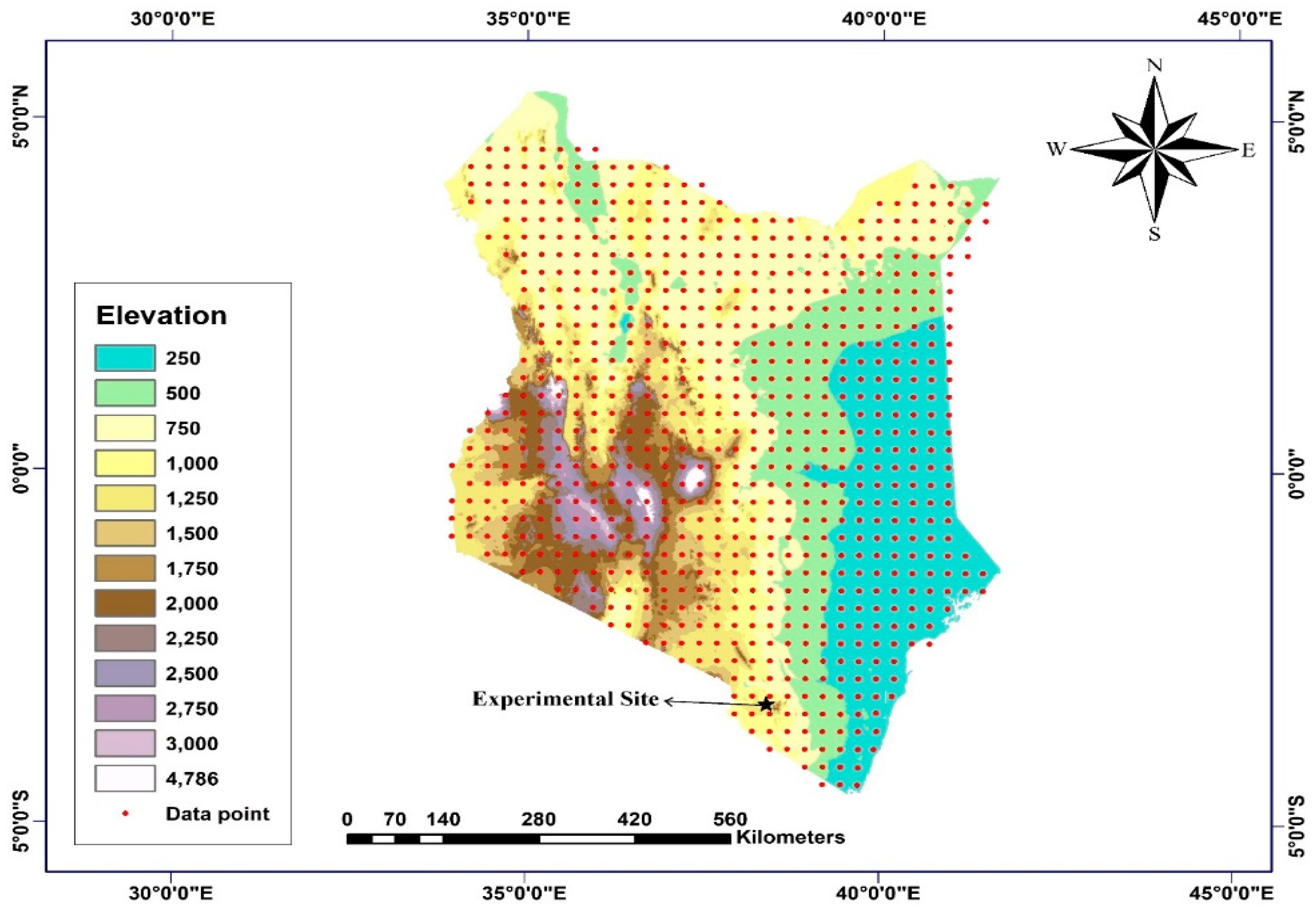
2.1. Experimental Data and Site Description

We utilized the dew collection database collected at Maktau (southeastern Kenya, 3° 25′33 S, 38° 8′22 E, 1060 m a.s.l.), which was previously reported by Tuure et al. [43]. In general, Kenya’s climate varies from tropical along the coastal areas and central highlands to temperate mostly in western parts and arid climate in the rest of the country according to the Köppen–Geiger climate classification. Therefore, about 80% of Kenya is located in arid and semi-arid areas [44,45,46]. It is characterized by low and erratic rainfall (100–1200 mm/year), high evapotranspiration rate, and a fragile ecosystem. The annual precipitation in Kenya increased from southwest towards highlands and central parts of the country and decreased in the northern and eastern parts [47,48]. Kenya has two rainy periods: the long-rain season that lasts from roughly March to May and the short rains from late October to early December [49]. Given the very few studies about dew, there is still a lack of knowledge addressing dew water harvesting in Kenya [43,50]. This is the first study estimating the dew collection potential in the whole of Kenya and evaluating the results against the experimental data.

The dew harvesting was performed from 15 February 2016 to 31 March 2017 (about 13 months). The dew was harvested on four types of condenser surface materials installed on 10 condensers. The surface materials were: (1) white polyvinyl chloride foil (PVC), (2) white polyethylene foil (PEW), (3) black polyethylene foil (PEB), and (4) OPUR. The condenser setup consisted of an aluminum frame supporting a 1 × 1-m² Styrofoam surface tilted at a 30° angle with respect to the ground surface. The Styrofoam backing used was 2.5 cm thick and functioned as thermal insulation, which prevented the absorption of long-wave radiation emitted from the soil and also convective heat flux in the air from warming up the foil surface and reducing evaporation of dew water from the condenser. All condensers were positioned facing west in order to lengthen the condensation time in the morning. The condensed dew water was drained gravitationally from the foil surface into a gutter which directed the water via a small tube into a small collecting tank or vessel. The water drainage was assisted by manually wiping the remaining water droplets to collect them and channel the resulting water into the gutter at sunrise.

2.2. Dew Formation Model and Simulation

2.2.1. Model Description

We evaluated a global dew formation model, which was developed by Vuollekoski et al. [28], against the experimental data described in Section 2.1. This is an energy-balance modeling approach which is similar to that developed by Pedro and Gillespie [37] and Nikolayev et al. [38] based on the mass–heat equation (a detailed description is found in the supplementary material (Section S1))

$$\frac{d{T}_c}{dt}=\frac{P_{rad}+P_{cond}+P_{conv}+P_{lat}}{\left(C_c{m}_c+C_w{m}_w+C_i{m}_i\right)}$$

(1)

where dT_c/dt is the change rate in the condenser temperature. C_c, C_w, and C_i are the specific heat capacity of condenser, water, and ice, respectively. Here, m_c, m_w, and m_i are mass of condenser, water, and ice, respectively. The right-hand side describes the heat exchange involved in the process: P_rad is the incoming and outgoing radiation, P_cond is the conductive heat exchange between the condenser surface and the ground, P_conv is the convective heat exchange, and P_lat is the latent heat released by the condensation or desublimation of water.

The model reads all input data for a given grid point and numerically solves the mass of water (m_w) and ice (m_i) and takes the preceding maximum value of m_w + m_i as the representative daily yield given in millimeters on a 1-m² condenser sheet (i.e., mm/m²/day equals L/m²/day). The model input parameters and their processing are described in detail in the supplementary material (Section S1). In this study, the term “dew yield” refers to the amount of water condensable on a 1m² condenser. The terms “dew occurrence” refers to the frequency of days that dew is observed on the condenser based on the model prediction.

2.2.2. Meteorological Input Database

The dew formation model input consists of meteorological data, which was obtained from the European Centre for Medium-Range Weather Forecast (ECMWF) Interim Reanalysis for a period of 40 years (1978–2018). Reanalysis combines a massive number of observations from a number of sources (satellite, radiosondes, aircraft, buoy data, stations, etc.) with a numerical weather prediction model to produce a coherent, long-term gridded data set of the atmospheric dynamic and thermodynamic state over the whole globe [51]. ERA-Interim has a native resolution of 0.75 degrees. Here, we consider the full years (1979–2018) and we also use data that were interpolated on a higher resolution (0.25 degrees, ~30 km) domain covering Kenya.

ERA-Interim contains two distinct types of fields, namely analysis fields and forecast fields [52,53]. Analysis fields are produced by combining short-range forecasts and observations whereas forecast fields are produced by the forecast model starting from an analysis. In ERA-Interim analysis fields are available every 6 h (00:00, 06:00, 12:00, and 18:00 UTC) and forecast fields are available every 3 h and hence can be used to fill in the gaps between the analysis. Furthermore, the forecast fields can either be instantaneous or accumulated over the forecast period.

The variables that are required for the dew formation model are the ambient air temperature (T_a), dew point temperature (DP), short-wave and long-wave surface solar radiation (R_sw and R_lw) and wind speed at 2 m extracted from horizontal and vertical wind components (U and V) at 10 m and surface roughness (z₀). From ERA-Interim, we extract 2-m T_a and DP from both the analysis and the instantaneous forecasts and obtain the short and longwave surface radiation as an accumulated forecast field.

2.3. Model versus Experimental Data Comparison

The model simulation results of the dew yield were taken at the grid point (about 7 km; 3° 45 S, 38° 20 E, 1047 m a.s.l.) which was the closest to the experimental site of dew harvesting (Figure 1). As described before, the experimental data were reported as total dew harvested on a daily basis (i.e., collected before the sunrise); therefore, the simulated yield was transformed to the cumulative dew yield consistently.

In order to make sure whether there is a linear correlation between the modeled and observed dew yield, we applied Pearson correlation (e.g., Benesty et al. [54]) and compared the absolute correlation coefficient (R²) with the critical values (e.g., Weathington et al. [55]) for the number of paired data at α = 0.05 (i.e., 95% confidence level). If |r| > critical value does hold for all paired data, then it proves the existence of linear correlation in the data set. Accordingly, a simple linear regression model (i.e., 2D model, one predictor, and one response) was assumed to describe the relationship between the observed and simulated dew yields [56,57,58]

Y_observed = m × X_simulated + c

(2)

where Y_observed is the observed dew yield and X_simulated is the simulated dew yield. In this simple regression, c was assumed to be zero and m was the regression constant between the observed and the simulated yield.

The comparison between observed and the simulated was represented by the Standard Error of regression Slope (SES), Residual Sum of Squares (RSS), Explained Sum of Squares (ESS), Total Sum of Squares (TSS), coefficient of determination (R²), Standard Deviations (SD), Mean Absolute Error (MAE), and Root Mean Square Error (RMS). The Standard Error of regression Slope (SES) represents the average distance that observed values deviate from the regression line. The smaller the “SES” value, the closer the values are to the regression line. Residual Sum of Squares (RSS = Ʃ (Y_obs − Y_est)²) indicates the residual variation of the observed values (Y_obs) in relation to the estimated values (Y_est) of the model. In essence, RSS is the amount of variance in the data set that is not explained by the regression model. The Explained Sum of Squares (ESS = Ʃ (Y_est − Y_obs)²), is a quantity that indicates the variation of the estimated values (Y_est) of the model in relation to its mean (Y_obs) and describing how much variation there is in the estimated values by the model compared to the Total Sum of Squares (TSS). The total Sum of Squares (TSS = Ʃ (Y_obs—Y_mean)²) is described as the sum of squares of deviation, which is the variation of the observed values, Y_obs, in relation to its mean, Y_mean. In some cases, the total sum of squares equals the sum of the two other sums of squares defined as TSS = RSS + ESS, when this relation does hold as in our case, the definition of R² is equivalent to

R² = ESS/TSS = (ESS/n)/(TSS/n)

(3)

where n is the number of observations. In this form, R² is expressed as the ratio of the explained variance (i.e., variance of the model’s predictions, ESS/n, to the total variance, TSS/n (i.e., sample variance of the dependent variable) [59].

2.4. Cluster Analysis

The model simulation was performed for the long-term period 1979–2018 by using a gridded domain that covered the whole regions of Kenya. In order to identify the major dew formation zones in Kenya, we applied cluster analysis (CA) on the scaled output data (i.e. multiplying the simulated yield by a factor obtained from the comparison between the observed and the simulated yields). Cluster Analysis (CA) is an effective statistical tool and technique that groups similar data points such that the points in the same group are more similar to each other than the points in the other groups and commonly used in atmospheric science [60,61]. We used hierarchical agglomerative clustering which consists of four main steps [62]:

• calculating the distance measure between all entries (data points);
• merging the two closest entries as a new cluster;
• recalculating the distance between all entries;
• repeating steps 2 and 3 until all entries are grouped into distinct groups (i.e., clusters).

Similarity measurement is a critical step in the hierarchical approach which influences the shape of the clusters [62]. The “Euclidean distance” is the most common distance metric and widely used in atmospheric science. The Euclidean distance between two objects i and j in a two-dimensional data matrix X (here the number of rows represented the number of spatial grid points in the model simulation domain and the number of columns represented the cumulative daily dew yield) is simply the squared difference between them for each of p variables, summed over the variables and k is the number of clusters [63]. This can be written as

$$d_{ij}=\sqrt{{\displaystyle \sum }_{k=1}^p{(x_{ik}-x_{jk})}^2}$$

(4)

The next step is merging the two closest entries (grid points) to form a new cluster based on a linkage criterion. There are some commonly used linkage criteria: single linkage, complete linkage, average distance, and Ward’s minimum variance methods, which differ in how the distances between entries are calculated and how the two closest entries are defined [64]. Here, we used Ward’s method for further analysis [65], which is the most frequent clustering technique used in climate research and it gives the most consistent clusters [61,66,67,68]. It calculates the means of all variables (the amount of dew) within each cluster, then calculates the Euclidean distance to the cluster mean of each case, and finally sums across all grid points [69].

In any CA, the optimal number of clusters is an important issue; however, there is no reliable and universally accepted method to decide the number of clusters and it can be a limitation when using CA, because the number of clusters also determines the amount of variance in each group. Therefore, the number of clusters should be selected so that both the number of groups and the variance within the groups are minimal. There are few suggestions about the optimum number of clusters [69,70,71]. Although, this information can be used as an indicator to decide the number of clusters a visual check of the result can still help to make the right decision. In our case, a few steps at n = 2, 3, 4, 5, and 6 are recommended as optimal numbers of clusters. By virtualizing all these steps, n = 3 (i.e., 3 dew zones) was found to be a better estimate for this study.

3. Results and Discussion

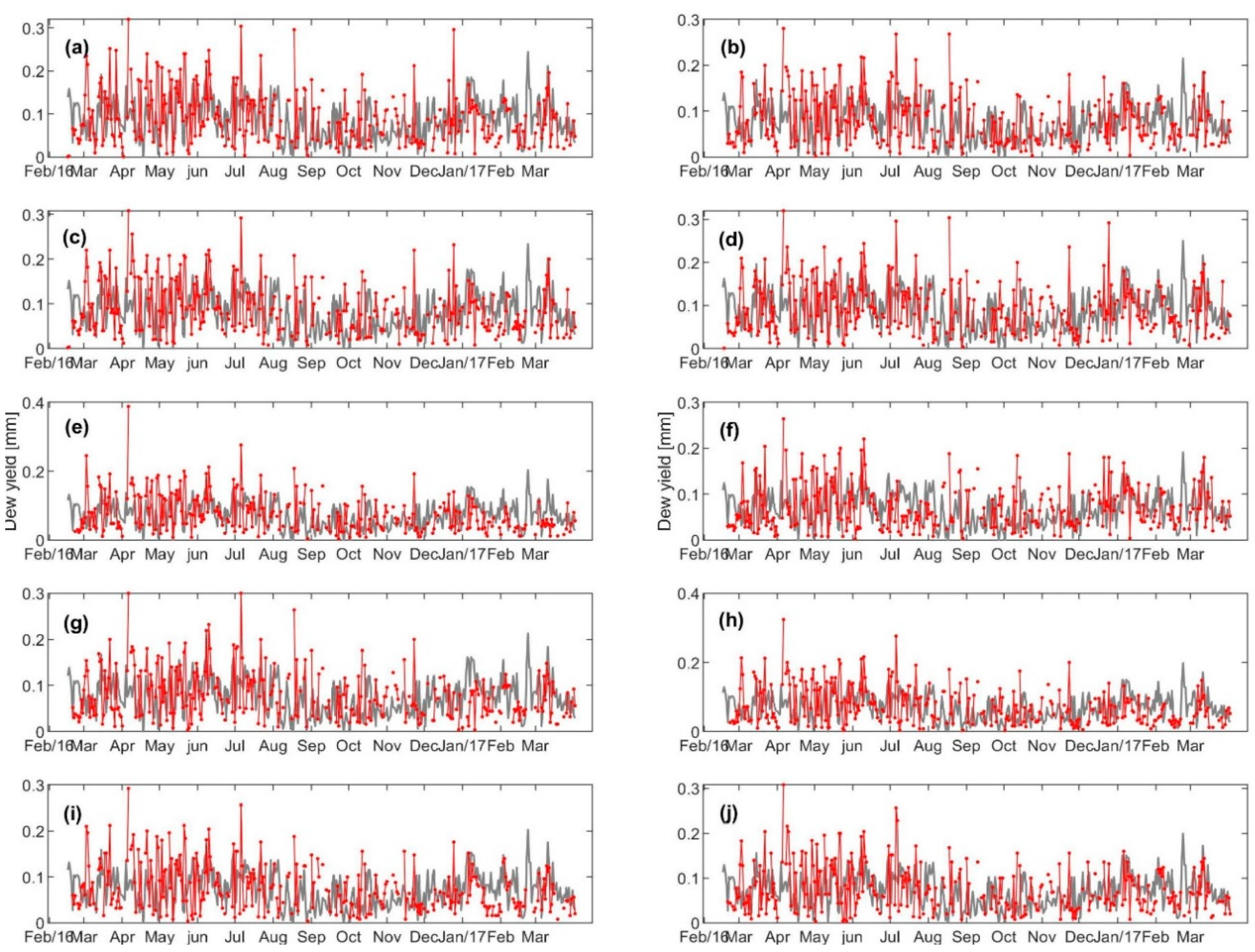
3.1. Dew Yields—Model Simulation versus Measurement

The comparison between the simulated and observed dew yields is presented in Figure 2, which covers the period 15 February 2016–31 March 2017. The model successfully predicted the dew occurrence observed during that period. However, on some days, the model predicted dew occurrence but there were no records reported for the actual dew occurrence. This suggests that the model can predict dew occurrence regardless of being collectible or not. In practice, negligible small dew yields are generally not harvestable because droplets might remain on the condenser surface and eventually evaporate before collection. It can be also that the model overestimates the dew yield. Quantitatively, the mean daily simulated dew yield was about 0.13 L/day. The observed mean yield was 0.07–0.09. Specifically, the model overestimated the dew yield for ~75% (70–78%) of the cases and underestimated about ~21% (18–28%) of the cases (

Table 1. Comparison simulated and observed dew yield during 15 February 2016–31 March 2017, using statistical parameters (Std: Standard deviation; MAE: Mean absolute Error; and RMSE: Root Mean Square Error) in the unit of mm/day.

Condenser	Mean	Max	Min	Std	MAE	RMSE	Underestimated (%)	Overestimated (%)
OPUR1	0.09	0.32	0.00	0.06	0.05	0.07	25.66	70.07
OPUR2	0.08	0.28	0.00	0.06	0.06	0.07	21.09	76.19
PVC1	0.09	0.31	0.00	0.06	0.05	0.07	24.75	71.57
PVC2	0.09	0.32	0.00	0.06	0.04	0.07	26.97	70.07
PVC3	0.08	0.39	0.00	0.05	0.06	0.07	19.23	78.32
PEwhite1	0.07	0.26	0.00	0.05	0.07	0.07	19.80	76.17
PEwhite2	0.08	0.30	0.00	0.05	0.06	0.07	21.69	72.88
PEwhite3	0.07	0.32	0.00	0.06	0.06	0.07	18.84	77.05
PEblack1	0.08	0.29	0.00	0.05	0.06	0.07	21.38	74.48
PEblack2	0.08	0.31	0.00	0.05	0.06	0.07	17.47	78.42
simulated	0.13	0.37	0.00	0.07	−	−	−	−

).

The disagreement between the simulated and observed dew yields could be due to several reasons. For instance, the model has two adjustable empirical parameters: h (heat transfer coefficient) and k (mass transfer coefficient). These are the functions of wind velocity and independent of time [29,39]. In particular, heat and mass transfer coefficients are important parameters in the model and determine how the condenser is cooled or heated by its surrounding air (h) and how water vapor condenses on the surface (k), which have an opposite effect during dew formation. Therefore, the overprediction indicates that the h value used in this study (i.e., parameterization by Richards [72], valid for u < 5 m/s) seems to be too small. More specifically, the model eliminates daytime dew due to incoming shortwave radiation and atmospheric longwave radiation that increases the condenser temperature and impedes condensation, it may also underestimate shortwave radiation at dusk and ignore the thermal lag effect present in reality and overestimate diurnal yield [31,72]. Moreover, in the model setup, we assumed there was no evaporation nor sublimation; however, dew was harvested once a day and it is probable that evaporation could occur before dew collection was performed.

In addition to the above discussion, there were some differences in the panel set up in the model and the experimental ones. For example, in the model setup, the condenser was at 2 m height and horizontally aligned whereas in the experimental setup it was placed at 0.5 m from the ground and tilted at a 30° angle. Hence, the latter could be affected by the soil heat flux and reduce the dew condensation. Most importantly, the distance between the closest grid point and the exact location of the dew collections was ~7 km, and dew is sensitive to the locals of the environment that might affect the dew yield and causes difference between simulated and observed yields.

However, a comparison of the cumulative sums of observed and simulated dew quantities (Figure 3) smooths down the daily variation and giving a better view of a strong correlation between the observed and simulated dew yields.

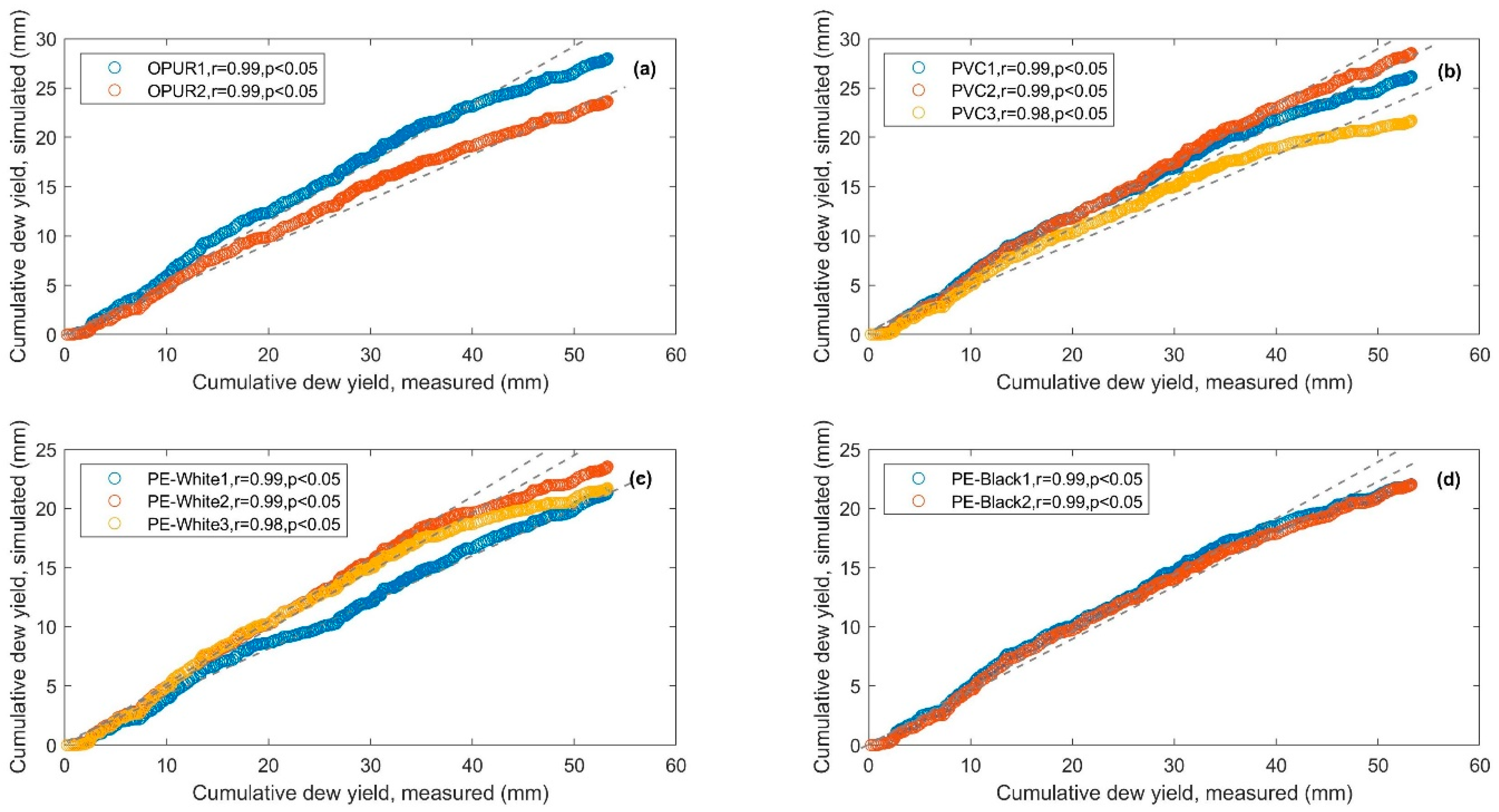
3.2. Simple Regression Analysis between Observed and Simulated Yields

The linear regression analysis and parameters are shown in

Table 2. Linear regression analysis and parameters during 15 February 2016–31 March 2017, in the unit of mm/day. (N: number of data pairs; SES: Standard Error of regression Slope; RSS: Residual Sum of Squares; ESS: Explained (regression) sum of squares; TSS: Total sum of squares and R2_ex indicates the correlation coefficient as explained variance).

Condenser	Slope	SES	N	RSS	ESS	TSS	R2_ex
OPUR1	0.66	0.06	304	1.51	0.58	1.18	0.49
OPUR2	0.58	0.05	294	1.05	0.44	0.90	0.49
PVC1	0.63	0.06	299	1.28	0.52	1.00	0.52
PVC2	0.68	0.06	304	1.41	0.61	1.09	0.56
PVC3	0.55	0.05	286	1.06	0.37	0.86	0.44
PEwhite1	0.52	0.05	298	0.93	0.35	0.72	0.49
PEwhite2	0.58	0.05	295	1.09	0.43	0.85	0.50
PEwhite3	0.54	0.05	292	1.07	0.36	0.90	0.41
PEblack1	0.55	0.05	290	0.98	0.38	0.79	0.48
PEblack2	0.54	0.05	292	0.94	0.37	0.79	0.47

. The coefficient of determination (R²) for all condensers’ material was in the range of 0.41–0.56. The highest correlation was observed for PVC2 (~0.55) and PVC1 (~0.53). The scaling factor (i.e., slope (m)) was in the range 0.52–0.68 (overall 0.58 ± 0.05). Specifically, the scaling factor for the OPUR condensers was 0.58–0.66 and for the PVC condensers it was 0.55–0.68. As for the PE white and black condensers, the scaling factor was 0.52–0.58.

A comparison between observed and scaled daily dew yields is presented in Figure 4. It is important to remember that, in the model setup, we calculated the dew yield for a sheet made of a suitable material such as low-density polyethylene (LDPE) or polymethylmethacrylate (PMMA). In reality, no clear variation between different types of condensers was observed; therefore, we scaled the model by using an average scaling factor of 0.6 ± 0.04 for it to be true for all condenser material.

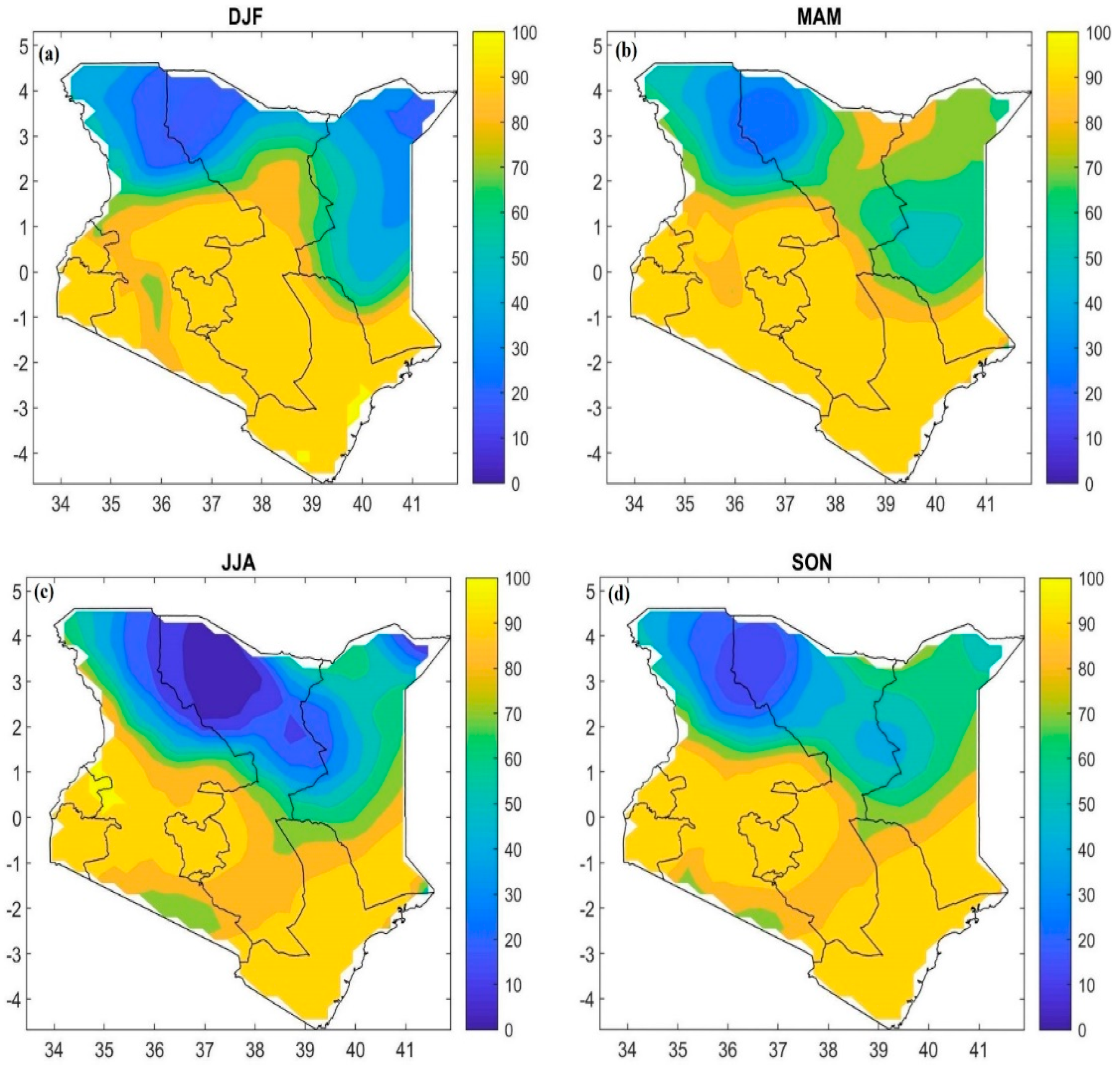
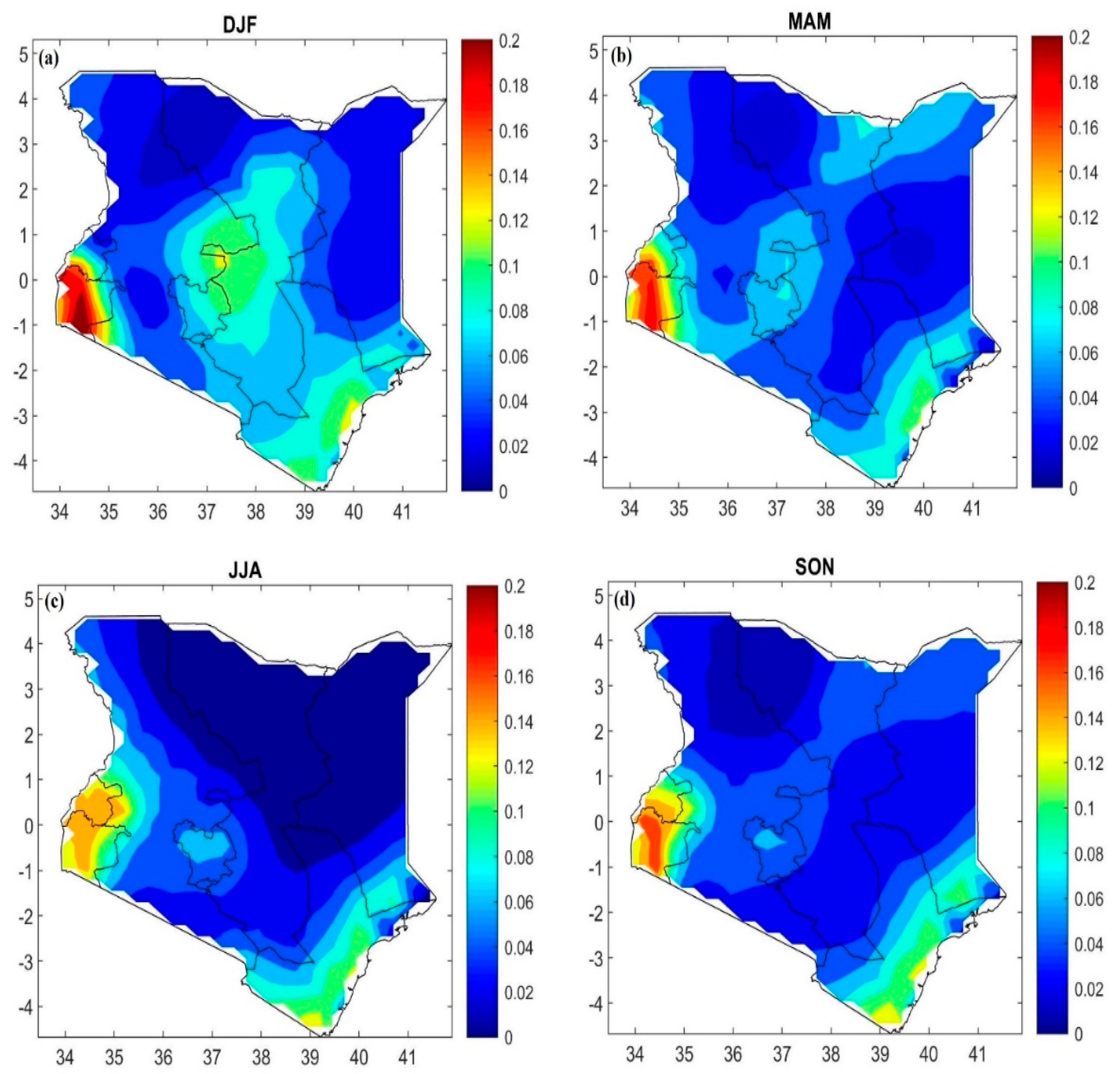
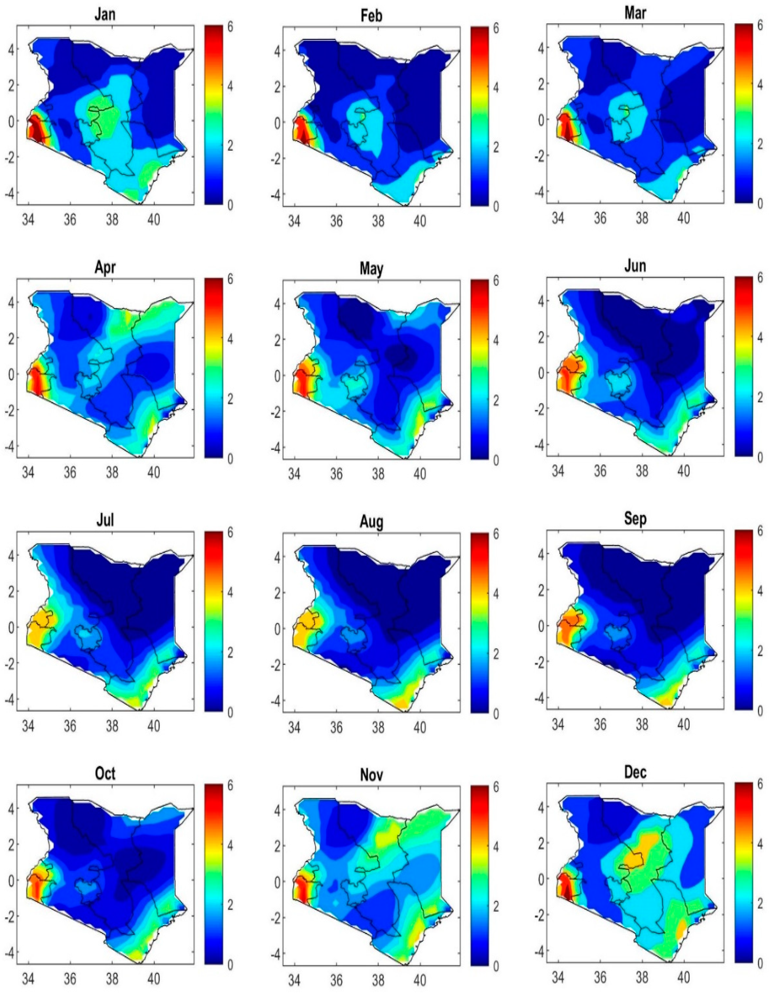
3.3. Long-Term Gridded Model Simulation—Spatial and Temporal Variations

After scaling of the simulated dew yield, i.e., scaling by a factor of 0.62, we performed long-term analysis for the spatial and temporal variations of the dew occurrence and yield over Kenya. According to this analysis, dew occurred almost everywhere in Kenya (Figure 5 and Figure S1). Figure 5 illustrates the seasonal occurrence of dew as a fraction of days with any dew yield. Figure S1 presents a similar seasonal occurrence of dew but for dew yield more than 0.1 L/m²/day. The frequency of dew occurrence was more than 70% (~265 days/ year) in the southern half of Kenya during all seasons. Whereas in the northern half of the country, the average dew occurrence was less than 40% (146 days). The smallest frequency of dew occurrence (<20% which is about 70 days) was observed in the north-western part. Seasonal variation of average dew occurrence in Kenya was not significant (62–72% days for summer and spring; respectively).

Limiting dew occurrence analysis to days with dew yield > 0.1 L/m²/day revealed a notable difference in both frequency and spatial scale for dew yield (Figure 5 and Figure S2). The average daily dew occurrence decreased by 35% with the highest decrease in spring (by ~40%) and lowest in winter (by ~29%). Moreover, the highest frequency of dew days was not in spring but in winter with ~45% (164 days). However, the seasonal variation was not pronounced. On the spatial scale, the areas with high dew occurrence were observed in the highlands and coastal regions. As expected, the areas and seasons with a high probability of dew occurrence also had high dew yields (Figure 6 and Figure 7). For example, winter, with an average of 0.09 L/m²/day, had the highest dew yields, whereas summer, with 0.06 L/m²/day, had the lowest dew yield.

Regarding the spatial distribution, the coastal areas of the Indian Ocean and Lake Victoria as well as the central mountain regions presented the highest dew yield throughout the year with mean cumulative daily dew varying in the range 0.1–0.2 L/m²/day. The remaining parts of the country did not show a comparable amount of dew yield (less than 0.04 L/m²/day). As for the monthly cumulative dew yield (Figure 7), the highest yields (8–12 L/m²/month) were observed in the western parts of Kenya (i.e., the Lake Victoria cost line) during autumn and early winter.

During the dry period (February–October), the dew occurrence was limited to only a small area in the coastal and mountain regions. In general, Kenya is an equatorial country; therefore, the seasonal temperature variations are small and the weather conditions depend on the seasonal movement of the Intertropical Convergence Zone (ITCZ). In particular, March is a transition month between north-easterly and south-easterly monsoons and November is a transition month between southeast and northeast monsoons. These two months have the highest relative frequencies of easterlies into Kenya [49], which bring moisture from the Indian ocean. On the other hand, during these periods, relative humidity and dew point showed a bimodal pattern as well as an increase in cloudiness. All these together with a significant reduction in wind speed (~2 m/s) due to stable weather conditions, favor the formation of dew in Kenya. From June to October, the south-east trade winds bring maritime air from the Indian Ocean [73]. Despite the maritime origin of the air due to declination in temperature, increasing T–DP, reduction in relative humidity, and stronger wind speed (~3 m/s) dew cannot form in large parts of the country.

The highest variation of dew occurrence and yield was mostly observed in northern parts of Kenya, which are dry regions (Figure S2). High variation in the Lake Victoria region is also interesting since this area showed a high potential for dew yield throughout the year.

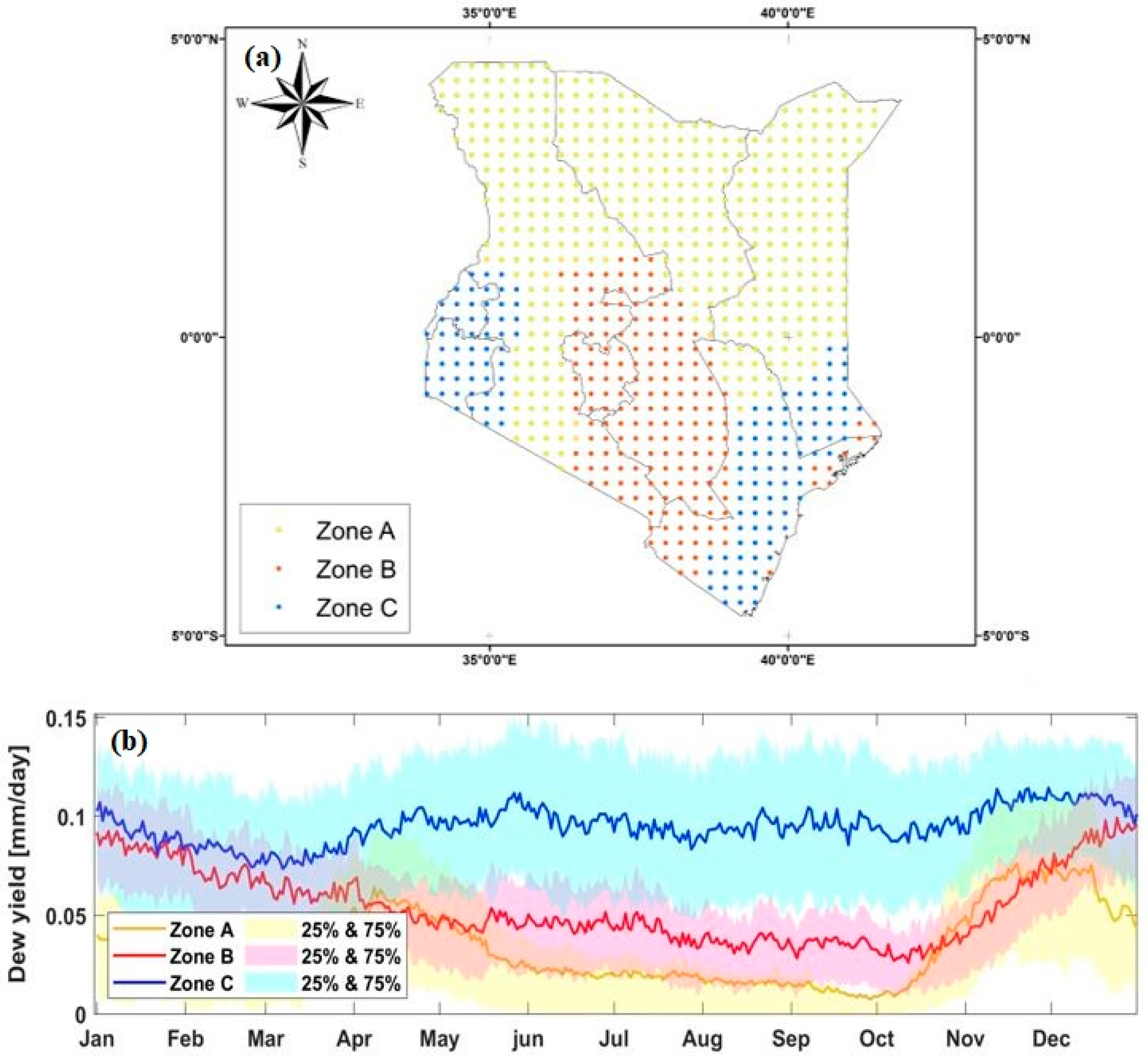
3.4. Dew Formation Zones—Cluster Analysis

In order to identify the major dew zones in Kenya, we applied Cluster Analysis (CA) on the scaled output data by assuming three clusters as an optimal number of dew formation zones (Figure 8a). Accordingly,

Table 3. Dew formation zones and their climate features (i.e., mean (min–max) values for meteorological parameters (T, DP, RH)) as well as statistical analysis for overall mean daily cumulative dew yield (i.e., std, 25th, 75th and 99th percentile and yearly max dew yield).

	Zone A	Zone B	Zone C
Region	Arid and Semi-Arid	Mountain region	Coastal region
Climate Features	Hot and dry	Mild and humid	Mild to hot and humid
Tmean (℃)	25 (24–28)	19 (11–26)	23 (22–25)
Td mean (℃)	16 (13–19)	15 (7–13)	18 (17–20)
RHmean (%)	60 (46–73)	69 (61–80)	74 (65–82)
Mean dew yield ± std (L/m2/day)	0.03 ± 0.02	0.05 ± 0.03	0.09 ± 0.02
25%	0.007	0.031	0.055
75% (L/m2/day)	0.049	0.074	0.129
99% (L/m2/day)	0.130	0.130	0.215
Max/year (L/m2)	>18	>25	>40

lists some quantitative information about the dew yield and related meteorological parameters (e.g., temperature, dew point, relative humidity). The seasonal cycle of the overall mean dew yield for each zone is illustrated in Figure 8b. Interestingly, the dew formation zones had a similar geographical distribution as that for the sources of moisture and climate zones. Furthermore, the mountains and the huge water bodies (i.e., The Indian ocean, Lake Victoria) played major roles in shaping the dew formation zones.

3.4.1. Dew Zone A–Arid and Semi-Arid Region

The first dew formation zone refers to the “arid and semi-arid” conditions that covered the northern and eastern parts of Kenya as well as the Rift Valley, which runs through Kenya from north to south separating the western and eastern highlands. This zone had a diverse range of topography and landscape including very dry lowlands in the north and east to humid highlands, large lakes, and forest (i.e., Mau forest, the largest forest complex in East Africa and one Kenya’s main water towers [74]). This zone was the driest and hottest area in Kenya, especially those parts located on low altitudes. The precipitation was sporadic and irregular, and the temperature varied between 40 °C during daytime and 20 °C during the nighttime with an annual mean of ~25 °C and small seasonal variation.

The maximum yearly dew that can be collected on 1 m² of a radiative condenser in this zone is ~18 L/m²/year, which is the lowest among all dew zones. The overall mean daily dew yield in this zone was about 0.03 ± 0.02 (maximum 0.13) L/m²/day, which was the lowest among the other dew zones. Correlation analysis showed that dew yield in this zone was strongly related to high T_d and RH and low wind speed as well as a small difference in T and DP (Figure S6). The long-term mean of the daily cumulative dew yield showed high values in late autumn and early winter (the peak was during November–December) and in spring (the peak was in April). Clearly, the highest dew yield accompanied the transition seasons, when ITCZ was changing its location by following the sun and prevailing easterlies that transfer moist air from the Indian ocean into this zone. It is important to mention here that air temperature did not change notably but the relative humidity was relatively high; therefore, the dewpoint is expected to be high and reach values closer to the air temperature. Furthermore, the wind speed was rather slow (~2.5 m/s at 2 m) (Figure S3). Therefore, dew can occur during these months.

During June–October is the southern hemisphere winter, which is colder than at other times in the year, but it is dry and the relative humidity is low. These conditions together with high wind speed (~3.5 m/s) prevent dew formation. Therefore, the dew yield declined and was somewhat ignorable (Figure 6, Figure 7 and Figure 8). Regardless of the climatic conditions during this period, the structure of topography may reduce dew condensation in some parts of this zone. For example, in the Rift Valley, the surrounding mountains or hills can trap the outgoing longwave radiations and reflect them back to the condenser surface, therefore reducing night-time cooling and impeding the formation of dew. The observed dew yield in Mexico City (i.e., 0.031 L/m²/day; [36]), which is located in the Valley of Mexico, can support our explanation here for this zone.

3.4.2. Dew Zone B—Mountain Region

The second dew formation zone (i.e., the mountain region) included Kenya’s Central Highlands region, which covered about 25% of our model domain (Figure 1). The maximum yearly dew yield in this zone was about 25 L/m²/year. The overall mean daily dew yield in this region was about 0.05 ± 0.03 (max: 0.13) L/m²/day, which is similar to the experimental studies conducted in Dodoma, Tanzania (south of Kenya) by (i.e., 0.05 L/m²/day; [32,75]).

In this zone, dew occurred throughout the year-round with the highest yields during December–January. During February, the dew yield declined to reach the lowest values in October (Figure 8b). That was a result of low relative humidity, low wind speed, and the increased difference between T and T_d. Moreover, the sky was almost always cloudy, especially in the evening, which reduces condensation. In other words, because of cloudiness, the shortwave radiation during daytime exceeded the longwave radiation during nighttime so that T-T_d increased and led to a low dew formation rate (Figure S4).

Indeed, other than the large or medium scale weather patterns, dew formation in this zone is mostly affected by the local weather conditions. In particular, the characteristics of the general circulation were generally modified at individual locations by regional and local factors, such as complex topography and large water bodies [76].

This could be another reason that dew did not occur in this zone. However, the wind speed showed a strong negative effect (R² = −0.76) on dew yield and seems that it had a significant role in the amount of dew (Figure S7).

3.4.3. Dew Zone C—Coastal Regions

The coastal zone is the smallest dew zone, which covered about 18% of the model domain in Kenya’s land; however, it had the highest yearly dew yield (~40 L/m²/year). The highest amount of mean daily dew yield (i.e., 0.09 ± 0.02 (max: 0.215) L/m²/day) was also observed in this zone with dew occurrence throughout the year (Figure 8b). The amount of dew yield in this zone is comparable with some coastal regions that have relatively similar climate: coastal south-western Madagascar (0.06–0.19 L/m²/day; [77]), Kothara, India (0.09 1 L/m²/day; [78]), Merlift, and south-west Morocco (0.1 L/m²/day; [79,80]).

This zone could be divided into two sub-zones: (1) the south-eastern part of Kenya and (2) the western part of Kenya. The first sub-zone was characterized by lowlands along with the coastlines of the Indian Ocean (Figure 1). The climate in this subzone was classified as tropical climate (i.e., very humid, and temperatures remain relatively constant all the year). The second subzone included the highlands located in the eastern portion of Lake Victoria (Figure 1). Kakamega forest in western Kenya is one of East Africa’s major rain forests [48]. The Rift Valley separated this subzone from the central mountain. Despite differences between these two locations from a topographic point of view, due to access to the vast water bodies (i.e., The Indian ocean and Lake Victoria), they have a significant potential for dew yield all year round.

Regardless of the high temperature, the Indian Ocean and Lake Victoria acted as a sufficient source of moisture for this zone. In addition, the weather was mainly stable and calm, the sky was usually semi-cloudy, and the mean daytime was about 9 h (Figure S5). The T-T_d and relative humidity had the highest correlation with dew yield in this zone (Figure S8). This means humidity and temperature controlled the level of dew yield here. However, the temperature was rather constant and high but, due to significant moisture content, dew can also occur during high-temperature conditions. Furthermore, the relative humidity (provided by moist trade winds and sea breeze) was high enough to compensate for the high temperature.

4. Conclusions

In this study, we used an energy balance model to estimate dew collection potential on artificial surfaces in Kenya as an arid/tropical country. The model was tested against a 13-month (1 March 2016 to 31 March 2017) experimental data conducted for 10 different condensers’ materials in Maktau, south Kenya. The model was used to simulate the dew yield for 40 years (1979–2018) to investigate the spatial and temporal variations of dew formation in Kenya and identify dew formation zones.

In general, the model overestimated the dew formation yield. Therefore, the model scaling was performed by introducing a factor of 0.6 to the estimated dew yields. The long-term model simulation for the dew formation was used to investigate the spatial and temporal variation of dew formation in Kenya. The results showed that the average dew occurrence in Kenya is ~265 days/year. However, not all days predicted by the model can be dew-harvestable. Considering dew yield > 0.1 mm/day, the annual dew occurrence was lowered by 35%. The dew showed a seasonal cycle with the maximum yields in winter (0.2 L/m²/day; Lake Victoria) and minimum in summer.

Based on our CA, we identified three dew zones. Zone A (i.e., arid and semi-arid), which covers more than half of Kenya’s land (57%) had the lowest potential for dew collection with average dew 0.05 mm/day (i.e., L/m²/day). Zone C (i.e., coastal region) had the highest potential of dew yield, with an average of 0.15 L/m²/day. However, this zone only covers 18% of the country. Zone B (i.e., mountain region) was similar to dew zone C, with a daily average dew yield of 0.9 L/m²/day. The maximum yearly dew yield in dew zone A-C was about 18, 25, and 40 L/m²/year, respectively. These results suggest that topography, sources of moisture (i.e., The Indian Ocean, Lake Victoria), and climate zones played major roles in the distribution of dew formation zones in Kenya. The highland and coastal areas showed the highest frequency of dew occurrence and yield throughout the year.

A precise prediction of dew occurrence and dew yield seems to be a challenge due to some inherent limitations in numerical models and meteorological input parameters. Thus, to achieve better estimations, the model needs to be calibrated with actual dew experiments in different climates. Improving input data resolution and involving more parameters in the calibration model is also recommended for future plans. However, uncertainly in results caused by model assumptions does not affect the spatial (dew zones) and temporal (seasonal variation) patterns in this study, and the results were in relatively good agreement with some experimental studies conducted for same the climates. This could confirm that the calibrated model has a reasonable performance in predicting dew in a long-term period, which is valuable for water management addressing atmospheric moisture in the form of dew.

References

1. Zala, B.; The Strategic Dimensions of Water 17. Water Security: Principles, Perspectives and Practices. 2013. Available online: http://bellschool.anu.edu.au/sites/default/files/publications/attachments/2016-07/zala_water_chapter_2013.pdf (accessed on 28 April 2021).
2. Human Development Report. Beyond Scarcity: Power, Poverty and the Global Water Crisis; United Nations: New York, NY, USA, 2006. [Google Scholar]
3. Tropp, H.; Jagerskog, A. Water Scarcity Challenges in the Middle East and North Africa (MENA); Human Development Paper; UNDP: New York, NY, USA, 2006. [Google Scholar]
4. Lekouch, I.; Muselli, M.; Kabbachi, B.; Ouazzani, J.; Melnytchouk-Milimouk, I.; Beysens, D. Dew, fog, and rain as supplementary sources of water in southwestern Morocco. Energy 2011, 36, 2257–2265. [Google Scholar] [CrossRef] [Green Version]
5. Michel, D.; Pandya, A.; Hasnain, S.I.; Sticklor, R.; Panuganti, S. Water Challenges and Cooperative Response in the Middle East and North Africa; Brookings Institution: Washington, DC, USA, 2012; Available online: https://www.brookings.edu/wp-content/uploads/2016/06/Water-web.pdf (accessed on 28 April 2021).
6. Mehryar, S.; Sliuzas, R.; Sharifi, M.; Van Maarseveen, M.F.A.M. The water crisis and socio-ecological development profile of Rafsanjan Township, Iran. In Ravage of the Planet IV; WITPRESS LTD: Southampton, UK, 2015; Volume 199, pp. 271–284. [Google Scholar]
7. Chahine, M.T. The hydrological cycle and its influence on climate. Nature 1992, 359, 373–380. [Google Scholar] [CrossRef]
8. Trenberth, K.E.; Smith, L. The Mass of the Atmosphere: A Constraint on Global Analyses. J. Clim. 2005, 18, 864–875. [Google Scholar] [CrossRef]
9. Hamed, A.M.; Kabeel, A.E.; Zeidan, E.S.B.; Aly, A.A. A technical review on the extraction of water from atmospheric air in arid zones. Int. J. Heat Mass Trans. 2010, 4, 213–228. [Google Scholar]
10. Raman, C.R.V.; Venkatraman, S.; Krishnamurthy, V. Dew over India and its contribution to winter-crop water balance. Agric. Meteorol. 1973, 11, 17–35. [Google Scholar] [CrossRef]
11. Rajvanshi, A.K. Large scale dew collection as a source of fresh water supply. Desalination 1981, 36, 299–306. [Google Scholar] [CrossRef] [Green Version]
12. Kidron, G.J.; Herrnstadt, I.; Barzilay, E. The role of dew as a moisture source for sand microbiotic crusts in the Negev Desert, Israel. J. Arid. Environ. 2002, 52, 517–533. [Google Scholar] [CrossRef]
13. Jumikis, A.R. Aerial wells: Secondary source of water. Soil Sci. 1965, 100, 83–95. [Google Scholar] [CrossRef]
14. Leopold, L.B. Dew as a source of plant moisture. Pac. Sci. 1952, 6, 259–261. [Google Scholar]
15. Kidron, G.J. Altitude dependent dew and fog in the Negev Desert, Israel. Agric. For. Meteorol. 1999, 96, 1–8. [Google Scholar] [CrossRef]
16. Alnaser, W.; Barakat, A. Use of condensed water vapour from the atmosphere for irrigation in Bahrain. Appl. Energy 2000, 65, 3–18. [Google Scholar] [CrossRef]
17. Richards, K. Observation and simulation of dew in rural and urban environments. Prog. Phys. Geogr. Earth Environ. 2004, 28, 76–94. [Google Scholar] [CrossRef]
18. Sharan, G.; Shah, R.; Millimouk-Melnythouk, I.; Beysens, D. Roofs as Dew Collectors: Corrugated Galvanized Iron Roofs in Kothara and Suthari (NW India). In Proceedings of the Fourth International Conference on Fog, Fog Collection and Dew, La Serena, Chile, 22–27 July 2007. [Google Scholar]
19. Odeh, I.; Arar, S.; Al-Hunaiti, A.; Sa’Aydeh, H.; Hammad, G.; Duplissy, J.; Vuollekoski, H.; Korpela, A.; Petäjä, T.; Kulmala, M.; et al. Chemical investigation and quality of urban dew collections with dust precipitates. Environ. Sci. Pollut. Res. 2017, 24, 12312–12318. [Google Scholar] [CrossRef] [PubMed] [Green Version]
20. Nilsson, T.; Vargas, W.; Niklasson, G.; Granqvist, C. Condensation of water by radiative cooling. Renew. Energy 1994, 5, 310–317. [Google Scholar] [CrossRef]
21. Muselli, M.; Beysens, D.; Marcillat, J.; Milimouk, I.; Nilsson, T.; Louche, A. Dew water collector for potable water in Ajaccio (Corsica Island, France). Atmos. Res. 2002, 64, 297–312. [Google Scholar] [CrossRef]
22. Clus, O.; Ortega, P.; Muselli, M.; Milimouk, I.; Beysens, D. Study of dew water collection in humid tropical islands. J. Hydrol. 2008, 361, 159–171. [Google Scholar] [CrossRef]
23. Muselli, M.; Beysens, D.; Mileta, M.; Milimouk, I. Dew and rain water collection in the Dalmatian Coast, Croatia. Atmos. Res. 2009, 92, 455–463. [Google Scholar] [CrossRef]
24. Sharan, G.; Clus, O.; Singh, S.; Muselli, M.; Beysens, D. A very large dew and rain ridge collector in the Kutch area (Gujarat, India). J. Hydrol. 2011, 405, 171–181. [Google Scholar] [CrossRef]
25. Khalil, B.; Adamowski, J.; Shabbir, A.; Jang, C.; Rojas, M.; Reilly, K.; Ozga-Zielinski, B. A review: Dew water collection from radiative passive collectors to recent developments of active collectors. Sustain. Water Resour. Manag. 2016, 2, 71–86. [Google Scholar] [CrossRef] [Green Version]
26. Tu, Y.; Wang, R.; Zhang, Y.; Wang, J. Progress and Expectation of Atmospheric Water Harvesting. Joule 2018, 2, 1452–1475. [Google Scholar] [CrossRef] [Green Version]
27. Hussein, T.; Sogacheva, L.L.; Petäjä, T. Accumulation and Coarse Modes Particle Concentrations during Dew Formation and Precipitation. Aerosol Air Qual. Res. 2018, 18, 2929–2938. [Google Scholar] [CrossRef] [Green Version]
28. Vuollekoski, H.; Vogt, M.; Sinclair, V.A.; Duplissy, J.; Järvinen, H.; Kyrö, E.-M.; Makkonen, R.; Petäjä, T.; Prisle, N.L.; Räisänen, P.; et al. Estimates of global dew collection potential on artificial surfaces. Hydrol. Earth Syst. Sci. 2015, 19, 601–613. [Google Scholar] [CrossRef] [Green Version]
29. Beysens, D.; Muselli, M.; Nikolayev, V.; Narhe, R.; Milimouk, I. Measurement and modelling of dew in island, coastal and alpine areas. Atmos. Res. 2005, 73, 1–22. [Google Scholar] [CrossRef] [Green Version]
30. Beysens, D. Estimating dew yield worldwide from a few meteo data. Atmos. Res. 2016, 167, 146–155. [Google Scholar] [CrossRef]
31. Tomaszkiewicz, M.; Najm, M.A.; Beysens, D.; Alameddine, I.; Zeid, E.B.; El-Fadel, M. Projected climate change impacts upon dew yield in the Mediterranean basin. Sci. Total Environ. 2016, 566–567, 1339–1348. [Google Scholar] [CrossRef]
32. Nilsson, T. Initial experiments on dew collection in Sweden and Tanzania. Sol. Energy Mater. Sol. Cells 1996, 40, 23–32. [Google Scholar] [CrossRef]
33. Gandhidasan, P.; Abualhamayel, H. Modeling and testing of a dew collection system. Desalination 2005, 180, 47–51. [Google Scholar] [CrossRef]
34. Jacobs, A.; Heusinkveld, B.; Berkowicz, S. Passive dew collection in a grassland area, The Netherlands. Atmos. Res. 2008, 87, 377–385. [Google Scholar] [CrossRef]
35. Maestre-Valero, J.F.; MartinezAlvarez, V.; Baille, A.; MartínGórriz, B.; GallegoElvira, B. Comparative analysis of two poly-ethylene foil materials for dew harvesting in a semiarid climate. J. Hydrol. 2011, 410, 84–91. [Google Scholar] [CrossRef]
36. Ernesto, A.-T.J.; Jasson, F.-P.J. Winter Dew Harvest in Mexico City. Atmosphere 2015, 7, 2. [Google Scholar] [CrossRef] [Green Version]
37. Pedro, M.; Gillespie, T. Estimating dew duration. I. Utilizing micrometeorological data. Agric. Meteorol. 1981, 25, 283–296. [Google Scholar] [CrossRef]
38. Nikolayev, V.; Beysens, D.; Gioda, A.; Milimouka, I.; Katiushin, E.; Morel, J.-P. Water recovery from dew. J. Hydrol. 1996, 182, 19–35. [Google Scholar] [CrossRef] [Green Version]
39. Nikolayev, V.S.; Beysens, D.; Muselli, M. A computer model for assessing dew/frost surface deposition. In Proceedings of the Second International Conference on Fog and Fog Collection, St John’s, NL, Canada, 15–20 July 2001; pp. 333–336. [Google Scholar]
40. Monteith, J.L. Dew. Q. J. R. Meteorol. Soc. 1957, 83, 322–341. [Google Scholar] [CrossRef]
41. Beysens, D. The formation of dew. Atmos. Res. 1995, 39, 215–237. [Google Scholar] [CrossRef]
42. Madeira, A.; Kim, K.; Taylor, S.; Gleason, M. A simple cloud-based energy balance model to estimate dew. Agric. For. Meteorol. 2002, 111, 55–63. [Google Scholar] [CrossRef]
43. Tuure, J.; Korpela, A.; Hautala, M.; Hakojärvi, M.; Mikkola, H.; Räsänen, M.; Duplissy, J.; Pellikka, P.; Petäjä, T.; Kulmala, M.; et al. Comparison of surface foil materials and dew collectors location in an arid area: A one-year field experiment in Kenya. Agric. For. Meteorol. 2019, 276–277, 107613. [Google Scholar] [CrossRef]
44. Makanga, J.T.; Ngondi, E.N. Status and Constraints of Wind Energy Resources Utilization in Kenya. Wind. Eng. 2010, 34, 255–262. [Google Scholar] [CrossRef]
45. Marshall, S. The water crisis in Kenya: Causes, effects and solutions. Glob. Major. E-J. 2011, 2, 31–45. [Google Scholar]
46. Billman, K. A Clean 5 Gallons a Day Keeps the Doctor Away: The Water Crisis in Kenya and Rwanda. Glob. Major. E-J. 2014, 75, 75–88. [Google Scholar]
47. Blank, H.G.; Mutero, C.M. The Changing Face of Irrigation in Kenya: Opportunities for Anticipating Changes in Eastern and Southern Africa (No. H030816); International Water Management Institute: Giza, Egypt, 2002. [Google Scholar]
48. Ayugi, B.O.; Wen, W.; Chepkemoi, D. Analysis of spatial and temporal patterns of rainfall variations over Kenya. J. Environ. Earth Sci. 2016, 6, 69–83. [Google Scholar]
49. Gatebe, C.K.; Tyson, P.D.; Annegarn, H.; Piketh, S.; Helas, G. A seasonal air transport climatology for Kenya. J. Geophys. Res. Space Phys. 1999, 104, 14237–14244. [Google Scholar] [CrossRef] [Green Version]
50. Patnaik, J.K. The potential of dew making as a source of water. In The Role of Water Resources in Development, Proceedings of the 13th Annual Symposium of the East African Academy, Nairobi, Kenya, 13–16 September 1977; Kenya National Academy for Advancement of Arts and Sciences: Nairobi, Kenya, 1977; Volume 60, p. 60. [Google Scholar]
51. Tampkins, A. A Brief Introduction to Retrieving ERA Interim via the Web and Webapi. 2017. Available online: http://indico.ictp.it/event/7960/session/4/contribution/28/material/slides/0.pdf (accessed on 28 April 2021).
52. Berrisford, P.; Dee, D.; Poli, P.; Brugge, R.; Fielding, K.; Fuentes, M.; Kallberg, P.; Kobayashi, S.; Uppala, S.; Simmons, A. ERA report series. In The ERA-Interim Archive; ECMWF—European Centre for Medium-Range Weather Forecasts: Reading, UK, 2011; Volume 2. [Google Scholar]
53. Dee, D.P.; Uppala, S.M.; Simmons, A.J.; Berrisford, P.; Poli, P.; Kobayashi, S.; Andrae, U.; Balmaseda, M.A.; Balsamo, G.; Bauer, P.; et al. The ERA-Interim reanalysis: Configuration and performance of the data assimilation system. Q. J. R. Meteorol. Soc. 2011, 137, 553–597. [Google Scholar] [CrossRef]
54. Benesty, J.; Chen, J.; Huang, Y.; Cohen, I. Pearson Correlation Coefficient. In Natural Computing Series; Springer: Berlin/Heidelberg, Germany, 2009; pp. 1–4. [Google Scholar]
55. Weathington, B.L.; Cunningham, C.J.L.; Pittenger, D.J. Understanding Business Research; Appendix B: Statistical Tables; John Wiley & Sons: Hoboken, NJ, USA, 2012. [Google Scholar]
56. Myers, R.H.; Myers, R.H. Classical and Modern Regression with Applications; Duxbury Press: Belmont, CA, USA, 1990; Volume 2. [Google Scholar]
57. Burton, P.; Gurrin, L.; Sly, P. Extending the simple linear regression model to account for correlated responses: An introduction to generalized estimating equations and multi-level mixed modelling. Stat. Med. 1998, 17, 1261–1291. [Google Scholar] [CrossRef]
58. Harrell, F.E. General Aspects of Fitting Regression Models. In Regression Modeling Strategies; Springer: Cham, Switzerland, 2015; pp. 13–44. [Google Scholar]
59. Archdeacon, T.J. Correlation and Regression Analysis: A Historian’s Guide; University of Wisconsin Press: Madison, WI, USA, 1994. [Google Scholar]
60. Güngör, E.; Özmen, A. Distance and density based clustering algorithm using Gaussian kernel. Expert Syst. Appl. 2017, 69, 10–20. [Google Scholar] [CrossRef]
61. Mimmack, G.M.; Mason, S.J.; Galpin, J.S. Choice of Distance Matrices in Cluster Analysis: Defining Regions. J. Clim. 2001, 14, 2790–2797. [Google Scholar] [CrossRef]
62. Nielsen, F. Introduction to HPC with MPI for Data Science; Chapter 8: Hierarchical Clustering; Springer: Berlin, Germany, 2016. [Google Scholar]
63. Fovell, R.G.; Fovell, M.-Y.C. Climate Zones of the Conterminous United States Defined Using Cluster Analysis. J. Clim. 1993, 6, 2103–2135. [Google Scholar] [CrossRef] [Green Version]
64. Stooksbury, D.E.; Michaels, P.J. Cluster analysis of Southeastern U.S. climate stations. Theor. Appl. Clim. 1991, 44, 143–150. [Google Scholar] [CrossRef]
65. Ward, J.H., Jr. Hierarchical grouping to optimize an objective function. J. Am. Stat. Assoc. 1963, 58, 236–244. [Google Scholar] [CrossRef]
66. Ahmed, B.Y.M. Climatic classification of Saudi Arabia: An application of factor—Cluster analysis. GeoJournal 1997, 41, 69–84. [Google Scholar] [CrossRef]
67. Yokoi, S.; Takayabu, Y.N.; Nishii, K.; Nakamura, H.; Endo, H.; Ichikawa, H.; Inoue, T.; Kimoto, M.; Kosaka, Y.; Miyasaka, T.; et al. Application of Cluster Analysis to Climate Model Performance Metrics. J. Appl. Meteorol. Clim. 2011, 50, 1666–1675. [Google Scholar] [CrossRef] [Green Version]
68. Kalkstein, L.; Tan, G.; Skindlov, J.A. An evaluation of three clustering procedures for use in synoptic climatological clas-sification. J. Appl. Meteorol. Climatol. 1987, 26, 717–730. [Google Scholar] [CrossRef] [Green Version]
69. Unal, Y.; Kindap, T.; Karaca, M. Redefining the climate zones of Turkey using cluster analysis. Int. J. Clim. 2003, 23, 1045–1055. [Google Scholar] [CrossRef]
70. Kaufmann, P.; Weber, R.O. Classification of Mesoscale Wind Fields in the MISTRAL Field Experiment. J. Appl. Meteorol. 1996, 35, 1963–1979. [Google Scholar] [CrossRef] [Green Version]
71. Burlando, M. The synoptic-scale surface wind climate regimes of the Mediterranean Sea according to the cluster analysis of ERA-40 wind fields. Theor. Appl. Climatol. 2009, 96, 69–83. [Google Scholar] [CrossRef]
72. Richards, K. Adaptation of a leaf wetness model to estimate dewfall amount on a roof surface. Agric. For. Meteorol. 2009, 149, 1377–1383. [Google Scholar] [CrossRef]
73. Sutherland, R.; Bryan, R.; Wijendes, D.O. Analysis of the monthly and annual rainfall climate in a semi-arid environment, Kenya. J. Arid. Environ. 1991, 20, 257–275. [Google Scholar] [CrossRef]
74. Parry, J.E.; Echeverria, D.; Dekens, J.; Maitima, J. Climate Risks, Vulnerability and Governance in Kenya: A Review; Commissioned by: Climate Risk Management Technical Assistance Support Project (CRM TASP), Joint Initiative of Bureau for Crisis Prevention and Recovery and Bureau for Development Policy of UNDP; UNDP: New York, NY, USA, 2012. [Google Scholar]
75. Vargas, W.; Lushiku, E.; Niklasson, G.; Nilsson, T. Light scattering coatings: Theory and solar applications. Sol. Energy Mater. Sol. Cells 1998, 54, 343–350. [Google Scholar] [CrossRef]
76. Ogallo, L.A. Dynamics of the East African climate. Proc. Indian Acad. Sci. Earth Planet. Sci. 1993, 102, 203–217. [Google Scholar]
77. Hanisch, S.; Lohrey, C.; Buerkert, A. Dewfall and its ecological significance in semi-arid coastal south-western Madagascar. J. Arid. Environ. 2015, 121, 24–31. [Google Scholar] [CrossRef]
78. Sharan, G.; Beysens, D.; Milimouk-Melnytchouk, I. A study of dew water yields on Galvanized iron roofs in Kothara (North-West India). J. Arid. Environ. 2007, 69, 259–269. [Google Scholar] [CrossRef]
79. Lekouch, I.; Kabbachi, B.; Milimouk-Melnytchouk, I.; Muselli, M.; Beysens, D. Influence of temporal variations and climatic conditions on the physical and chemical characteristics of dew and rain in South-West Morocco. In Proceedings of the 5th International Conference on Fog, Fog Collection and Dew 2010, Münster, Germany, 25–30 July 2010; pp. 43–46. [Google Scholar]
80. Lekouch, I.; Lekouch, K.; Muselli, M.; Mongruel, A.; Kabbachi, B.; Beysens, D. Rooftop dew, fog and rain collection in southwest Morocco and predictive dew modeling using neural networks. J. Hydrol. 2012, 448–449, 60–72. [Google Scholar] [CrossRef]
Figure 1. A map of Kenya with the geographical topography and the model domain grid points. The location of the experimental site is indicated by an arrow.
Water 13 01261 g001
Figure 2. Time series of daily dew yield showing the comparison between the model simulation (unscaled yield) and the observed dew yield during 15 February 2016–31 March 2017: (a) OPUR condensers, (b) PVC condensers, (c) PEwhite condensers, and (d) PEblack condensers.
Water 13 01261 g002
Figure 3. Correlation (Pearson’s correlation, 1:1 relationship) between the cumulative sum of the observed and the simulated dew yields during a 13-month measurement period for all condensers: (a) OPUR condensers, (b) PVC condensers, (c) PE-White condensers, and (d) PE-Black condensers. The gray dashed lines are the best linear fits.
Water 13 01261 g003
Figure 4. Time series of the cumulative daily dew yield showing the comparison between the model simulation (scaled yield) and the observed dew yield during 15 February 2016–31 March 2017: (a) OPUR1, (b) OPUR2, (c) PVC1, (d) PVC2, (e) PVC3, (f) PEwhite1, (g) PEwhite2, (h) PEwhite3, (i) PEblack1, (j) PEblack2.
Water 13 01261 g004
Figure 5. Dew occurrence maps showing the percentage of dew occurrence days during 1979–2018: (a) winter (December, January and February), (b) spring (March, April and May), (c) summer (June, July and August), and (d) autumn (September, October and November).
Water 13 01261 g005
Figure 6. Dew yield maps showing the overall mean cumulative daily dew yield (mm/day) during 1979–2018: (a) winter (December, January and February), (b) spring (March, April and May), (c) summer (June, July and August), and (d) autumn (September, October and November).
Water 13 01261 g006
Figure 7. Dew yield maps showing the overall mean monthly dew yield (mm/month) during 1979–2018. Each subplot represents the dew yield map for a certain month.
Water 13 01261 g007
Figure 8. (a) Dew formation zones based on the cluster analysis of the daily cumulative dew yield during 1979–2018 and (b) corresponding long-term mean seasonal variation of the cumulative daily dew yield. Note that color-coding on both figures is the same and corresponds to the dew formation zones: (yellow) dew zone A (arid and semi-arid region), (red) Zone B (mountains region), and (blue) Zone C (coastal region). The shaded parts around the lines represent the 25th and 75th percentile of daily dew yields for each cluster, and colors are the same as clusters.
Water 13 01261 g008