
Horizontal Distribution of Deep Sea Microplankton: A New Point of View for Marine Biogeography
by
 ,
,
Jessica Vannini
1,2, 
Lidia Yebra
2,
Antonia Granata
3,
Letterio Guglielmo
4,
Salvatore Moscatello
1 and
Genuario Belmonte
1,* 1
Department of Biological and Environmental Sciences and Technology, University of Salento, 73100 Lecce, Italy
2
Oceanographic Center of Málaga, Spanish Institute of Oceanography, 29640 Fuengirola, Spain
3
Department of Biological, Chemical, Pharmaceutical, and Environmetnal Sciences, University of Messina, 98100 Messina, Italy
4
SZN Zoological Station Anton Dohrn, Villa Comunale, 80121 Naples, Italy
*
Author to whom correspondence should be addressed.
Water 2021, 13(9), 1263; https://doi.org/10.3390/w13091263
Submission received: 15 March 2021
/
Revised: 26 April 2021
/
Accepted: 26 April 2021
/
Published: 30 April 2021
(This article belongs to the Special Issue Implementation of Biodiversity and Ecosystem Services in Marine Ecosystem Management)
Abstract
:An investigation on microplankton composition and spatial distribution has been carried out around Italian seas. The analysis of 53 samples, collected in 2017 at two depths in 27 different stations, has led to a scenario of horizontal distribution of microplankton. Dinophyta and Ciliophora were chosen as representatives of the whole microplankton community. A total of 60 genera were identified. Cluster analysis of data regarding taxa presence and abundance led us to recognize that similarities between surface stations were more evident than those between deep ones. Furthermore, we conducted an inter-annual comparison with available data from the South Adriatic Sea (2013, 2015). The higher dissimilarity between deep sea samples was also confirmed in a relatively smaller geographic area. The dissimilarity of deep-sea samples does not correspond to a higher habitat diversification, in terms of abiotic parameters. It has been suggested that the negligible biological connectivity in the deep, for those micro-organisms not able to perform wide spatial migrations, could produce such a biological diversification.
1. Introduction
Microplankton is considered fundamental for pelagic marine ecosystem functioning [1]; this notwithstanding, studies on this marine compartment are still largely insufficient. Microplankton is composed mostly by unicellular organisms with short life cycles which allow the community composition to change faster than the metazoan plankton. Most single components (species) are even able to disappear from the water column by producing resting stages which rest on the bottom before hatching a mobile form on the return of favorable conditions [2,3]. Thanks to the presence of resting stages, locally even more abundant than corresponding active stages [4], microplankton organisms are considered to be geographically widespread and sometimes present everywhere [5,6]. This generalization, however, derives mainly from studies of freshwater organisms, and knowledge of adaptation and distribution mechanisms of unicellular organisms in the sea abruptly decreases from the coastline towards the pelagic habitat. Dale [7] and Taylor [8] calculated that only 13–16% of about 2000 marine Dinophyta species were known to produce resting stages, and this trait of the life cycle has been described only in 3 species of marine Ciliophora Oligotrichida from a total of 141 known species [9,10,11]. Although these numbers are continuously updated (see [12] for recent lists of marine plankton species producing cysts), they are still not enough to justify that species distribution and circulation in the open sea should be based on cyst dispersal as it occurs for freshwater environments. Microplankton, in addition, performs vertical migration only for short distances [13] thus not comparable to vertical daily migrations of hundreds of meters typical of mesoplanktonic crustaceans, and/or horizontal movements of kms typical of nekton. These facts strongly suggest the isolation of local communities. If such a supposition is correct, microplankton distribution might be characterized by a geographic partitioning someway independent of abiotic features.
Ocean pelagic biogeography is based on information regarding large-sized organisms [14], but when the size of organisms is small enough, (generally that of unicellular microplankton) any geographical partitioning in species and diversity distribution seems to be unrecognizable [15].
A general rule correlates the trait-functioning of unicellular plankton (e.g., the cell size, or the trophic role) with the concentration of nutrients in the water, thus allowing the partitioning of large geographical areas [16]. In oligotrophic waters, predators of small sized phytoplankton are mostly large unicellular zooplankton, such as Ciliophora, which in turn are prey for Metazoa [17]. In waters with higher trophic status, large-sized phytoplankton thrive, and these are direct food for Metazoa. This general model proposes a simplification of the trophic web which could correspond to differences in species richness and diversity. On this basis, more species can be predicted in the unicellular plankton of oligotrophic intertropical oceans than in mesotrophic polar ones. However, we should also expect more species in the euphotic zone than in deep waters, where photosynthetic producers are absent.
Another general rule, however, adds complexity to the frame. The species richness and the community composition depend also on the geographic extension considered. In fact, genetic drift and speciation are favored at extremities of a spatial distribution, when the geographic extension is large enough to reproductively isolate sub-populations at margins [18,19].
Therefore, ocean extensions that are apparently homogeneous as the deep environment, should show a biogeographic partitioning different from the surface layer. The study of unicellular plankton (microplankton) could help in understanding this frame because spatial segregation should be enhanced in small-sized species, whose populations suffer the impossibility of inter-connecting themselves on the geographic scale commonly used for macro-organisms. Unicellular plankton, in fact, are considered unable to migrate to suitable areas, if required, as metazoan plankton do [20], and for this reason their species assemblages should be better linked to biological features (e.g., reproduction, competition and other species interaction) than to abiotic ones.
The community structure of sub-surface microplankton in a station of the Gulf of Naples has been reported as constant over a time period of 4 years, although subjected to seasonal variation in species composition and organism abundance [21]. In a study of the seasonal and inter-annual variability of microplankton at two depths of a unique station in Villefrance Bay (NW Mediterranean Sea) the statistical clustering of microplankton assemblage at 50 m depth showed a higher variability (more time units) than the sub-surface ones [22]. In a study on the Ionian Coast of Sicily (Central Mediterranean), notwithstanding the evident homogeneity of the water column conditions in that study, the Diversity (H’) of Tintinnina assemblage at 35–50 m depth was higher than that of the surface [23]. These studies, although carried out on small water columns, and in single stations, clearly depict a tendency of surface microplankton to be more uniform than the deep ones in long time observations. Variability of environmental conditions in the epipelagos (mostly in the first 100 m layer) justifies the different arrangements of assemblages at different depths, but below 200 m the environment does not show such variations and community composition is expected to be more homogeneous.
The present study aims to compare the horizontal variability of surface microplankton with that of deep waters (down to 500 m depth), to verify if the mesophotic community assemblages can be partitioned in local subcommunities, in some way corresponding to those of the surface or, on the contrary, if a possibly different geographic distribution of microplankton at different water depths exists and why. The availability of data from preceding collection campaigns, in addition, represented a possibility to explore the variability in the time scale.
2. Materials and Methods
2.1. The Geographic Area
The area object of the study is that, around the Italian Peninsula, in the center of the Mediterranean Sea. This basin is positioned in the warm temperate geographic area of the planet and it was biologically colonized by the Atlantic Ocean after the Messinian dry crisis [24]. The studied area comprised either shallow, epicontinental seas (such as the north Adriatic), or deep seas (such as Tyrrhenian and Ionian seas) where the bottom is at more than 2000 m depth. The maximum concentration of Chla reaches surface layers in shallow areas, but this is around 60–80 m below the sea surface in the deeper parts [25]. For such a reason, the variability of environmental conditions is maximum in the first 100 m of the water column. Below the depth of 200 m the main features (Salinity, Temperature, pH, Oxygen concentration) are considered practically unvariable, and absence of sunlight and of active phytoplankton add another element of homogeneity to the environment. Finally, the pressure also varies to a lesser extent, doubling from 200 to 400 m (at surface the pressure increases of 20 times in the first 200 m). The microplankton assemblage of the highly variable layer (epipelagos) has been collected to be compared with that of the mesopelagic layer (200–500 m) with the aim to identify any difference, if it exists.
2.2. Sampling
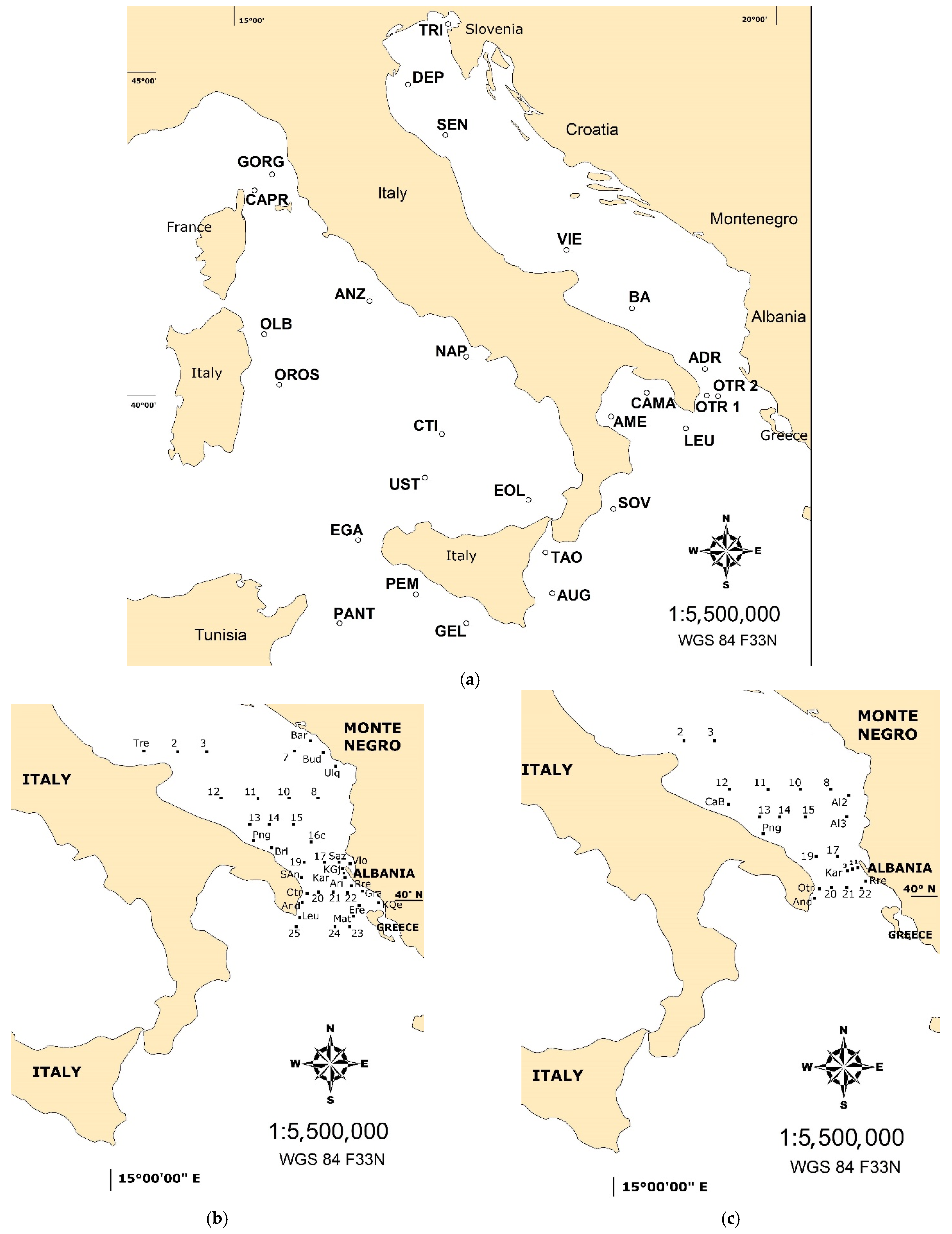
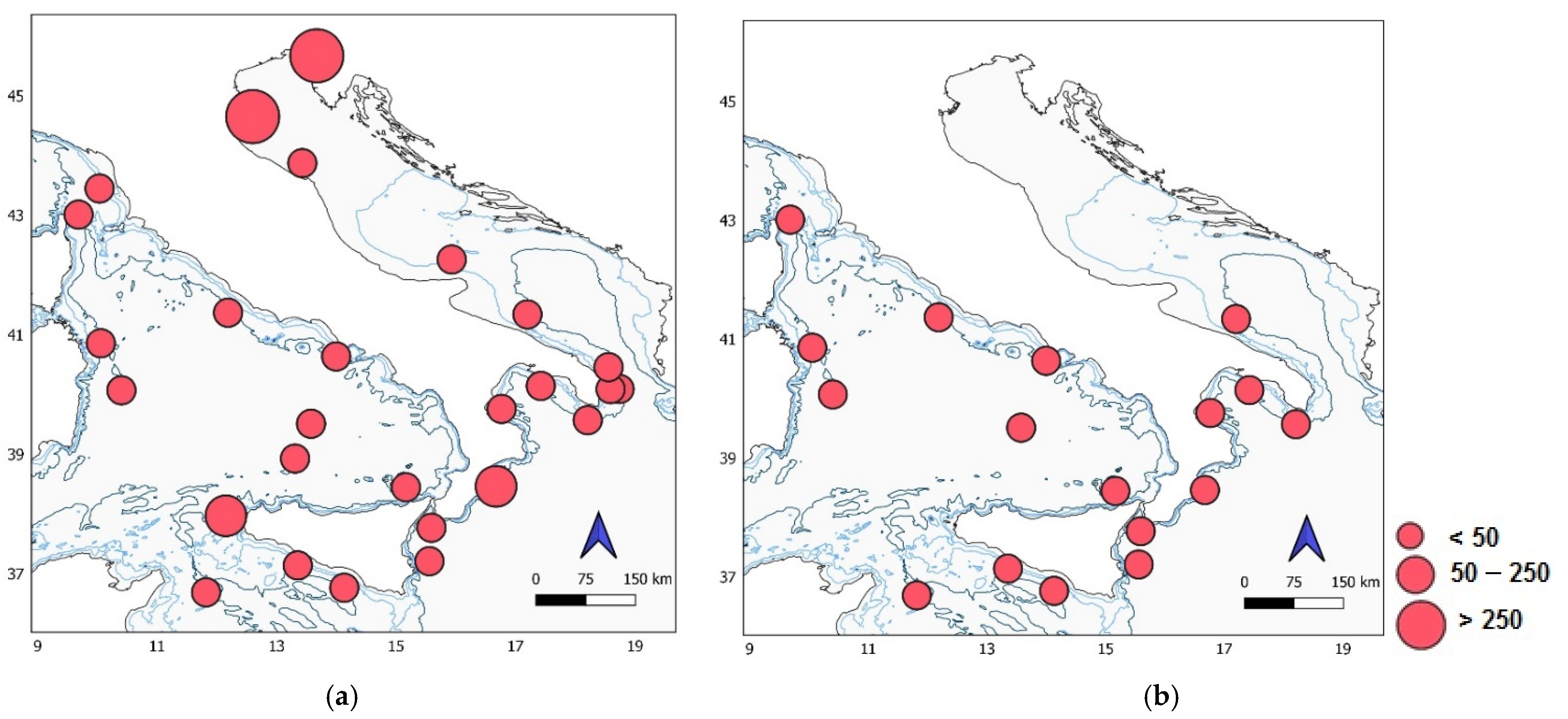
An oceanographic cruise was carried out with the Research Vessel “Minerva 1”, in the period 4 July–12 August 2017, during which 53 microplankton samples were collected from two depths in 27 stations around the Italian peninsula (Figure 1a). The station UST (Ustica) gave the only surface sample. All samples had a volume comprised between 5 and 10 L of sea water. They were collected with a carousel of 12 L Niskin bottles whose closure was commanded at the selected depth, from the vessel.
Samples were collected in the epipelagic layer, at 2–4 m below the sea level, and in the mesopelagic layer, between 200 and 500 m depth, according to the extension of the water column at each station. When bottom depth was less than 500 m, samples were collected, in any case, at not less than 3 m from the bottom (Table S1). Then, the collected samples were gently concentrated with a 10 μm mesh and placed in 200 mL bottles. Samples were fixed with formalin (2% of final concentration). The carousel used for the collection of samples was equipped with a multiparametric probe for the measurement of Temperature, Depth, Salinity, and Chla concentration along the water column at each station.
Due to the methodological correspondence of sample collection (see below), the results of the 2017 cruise were compared with data of two preceding cruises limited to the South Adriatic Sea (May 2013, 39 stations, 78 samples Figure 1b, and March 2015, 24 stations, 48 samples Figure 1c; see also [25] and Supplementary Material Tables S2 and S3). Additionally, in these two previous cruises, all samples had a volume of between 5 and 10 L of sea water. The water volume of each sample was filtered (immediately after the collection) throughout a sieve with mesh size of 10 μm and then rinsed and passed from the sieve to a 50 mL Falcon tube directly with ethanol 95% (for a final concentration of the sample at Et-OH 80–85%). From 2013 and 2015, only the data for temperature and salinity are available (Supplementary Material Tables S4 and S5).
The 2013 cruise was carried out in May, and the 2015 cruise in March; both covered only the South Adriatic Sea, where samples and hydrographic data were collected from 39 and 24 stations, respectively, at the surface and close to the bottom in each station. Deep collection points of these two cruises considered together ranged between 23 and 1168 m below the sea level.
The 2013–2015, samples have been used in this study to increase the available data for the description of horizontal zonation of microplankton in a smaller geographic area, the South Adriatic Sea, and for the characterization of microplankton communities at different depths along the water column.
2.3. Taxonomic Analyses
The samples collected were analyzed under an inverted microscope (125–400 magnification) to establish the taxa composition of microplankton assemblages. The counts and identification of organisms were executed after a 12 h sedimentation in a Petri dish hosting an aliquot of the sample with the water layer having the thickness of 0.5–0.8 cm. Additionally, due to the concentration of each sample in a small final volume of 35–50 mL (a Falcon tube), and the possibility to analyze aliquots each of up to 10 mL (under the inverted microscope), samples were analyzed entirely. The count of very abundant taxa relied upon 3 aliquots of previously gently mixed sample, and the whole sample was analyzed for the count of rare taxa.
To have the maximum reliability in the comparison analyses, the present study focused on genera of Dinophyta and Ciliophora, recognized as the most represented in terms of taxa, with the assumption that identification based on genus is more reliable when comparing data sets that are distant in time [26], due to possible differences in analyst capability. In addition, analysis based on genus abundance and distribution are considered very similar with data based on species in biodiversity assessments [27]. The two taxa selected, one autothrophic and one heterothrophic, also adequately represent the ecological variety of the microplankton assemblage.
2.4. Statistical Analyses
Taxa abundance data (individuals L−1) of 2017 were root-transformed to produce a Bray–Curtis similarity matrix. Then, we performed Hierarchical cluster analysis and non-metric Multi-Dimensional Scaling (n-MDS) with PRIMER 6 version 6.1.11 (PRIMER-e, Auckland, New Zealand) [28]. Rare species (those that not occurred in more than three stations) were excluded from Hierarchical Cluster and nMDS analyses to avoid overfitting.
Clustering of stations was achieved based on a preliminary analysis of similarity between samples collected very close to each other (in horizontal or in vertical sense), thus considered as representing uniform spatial groups. The medium value of similarity obtained from this preliminary analysis (50%) was adopted as the similarity value to include or separate different stations in the same spatial cluster.
For each of the different groups resulting from the n-MDS analysis, the contribution percentage was determined with one-way SIMPER analysis and a cut-off criterion of less than 90% contribution was applied to the similarity value.
From abiotic data the BEST test was performed to study relationships between biological and environmental variables and Principal Component Analysis (PCA) were performed to obtain distribution of samples based on abiotic features. A T-S diagram was produced to individuate water masses with Ocean Data View software (ODV, Alfred Wegener Institute, Bremerhaven, Germany) [29].
3. Results
3.1. Hydrographic Conditions
3.1.1. Cruise 2017
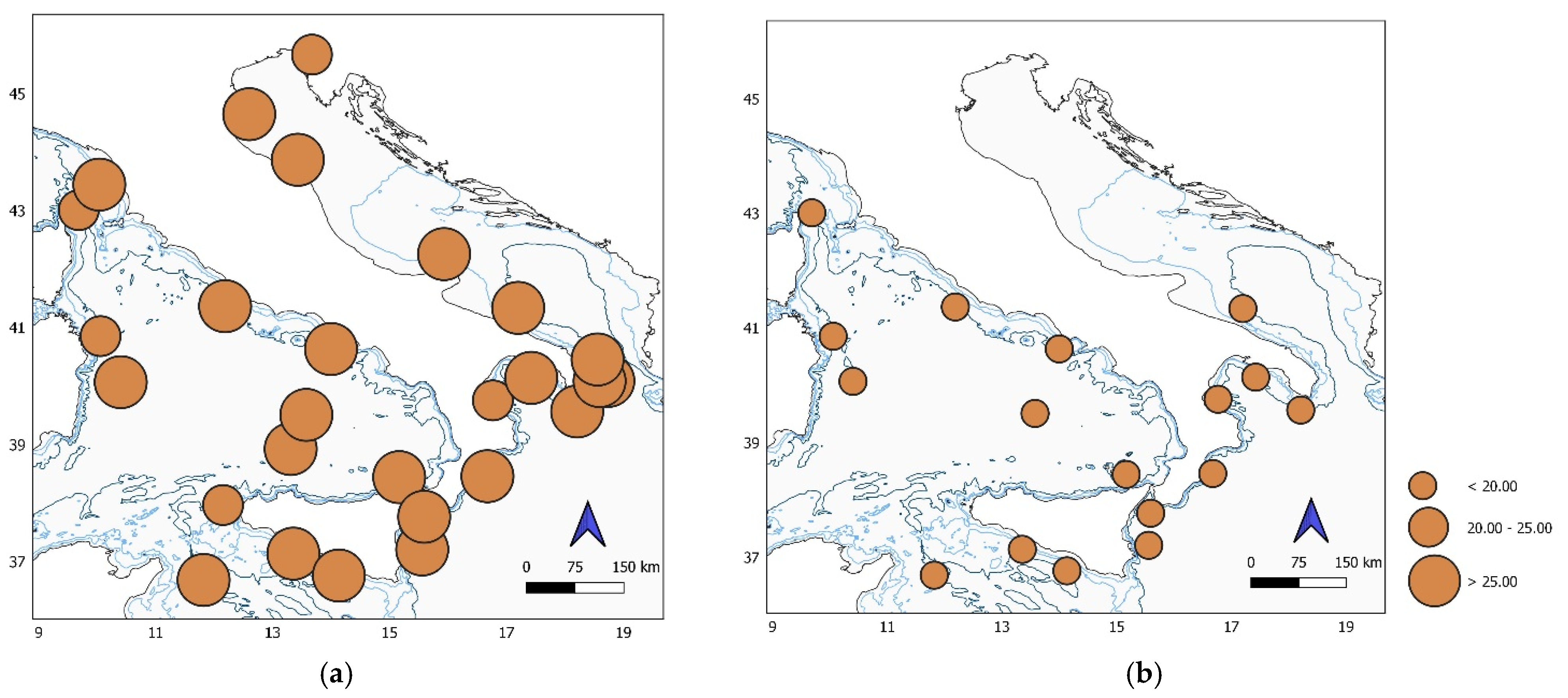
As usual, for the summer period (4 July–12 August 2017), epipelagic waters were warmer; in addition, they also showed a wider temperature range than mesopelagic waters (Figure 2a,b). Indeed, the highest surface temperature was recorded at station SEN (Senigallia) (27.9 °C) and the lowest at TRI (Trieste) and OLB (Olbia) (23.9 °C) with a difference of 4 °C. Mesopelagic waters (below 200 m), on the contrary, were homogenously cooler and oscillated by only 0.5 °C between 13.9 and 14.4 °C in the whole station set (Table S1).
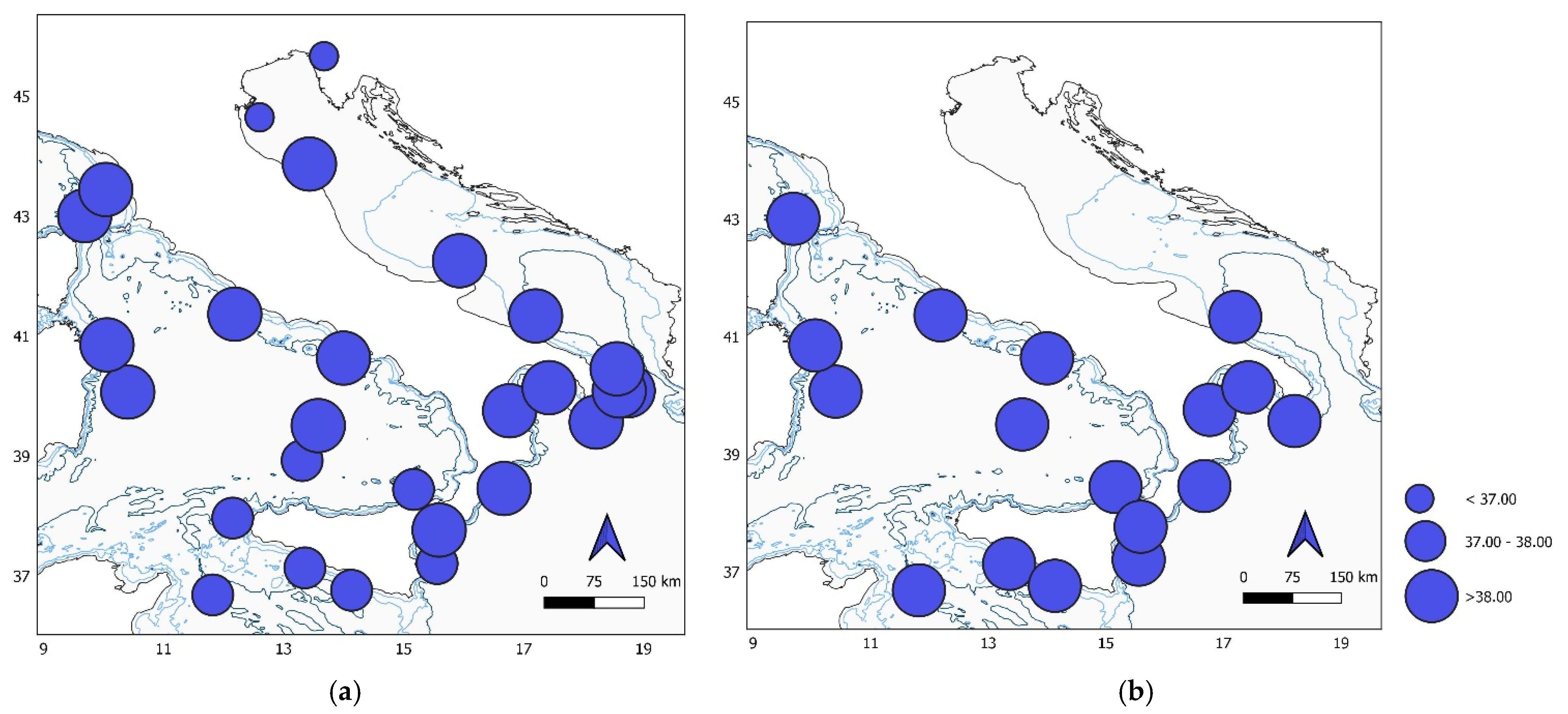
The highest surface salinity (39.1) was recorded at station BA (Bari), notably higher than the lowest salinity (34.4) measured at station DEP (Po River Delta). Below the first 200 m, in the mesopelagic layer, salinity was relatively homogeneous, ranging between 38.7 and 38.9 in all the stations (Supplementary Material Table S1, Figure 3a,b).
The Chla concentration in surface waters was generally low, ranging between 0.00 and 0.04 µg L−1 and reaching a peak only in the North Adriatic (DEP and TRI) with 0.20 µg L−1. The maximum Chla concentration at each station was found at 24–50 m depth with the highest values of the whole study in the North Adriatic Sea (0.30 and 0.66 µg L−1 at stations DEP MD and TRI MD, respectively). The Chla concentration in mesopelagic waters (below 200 m) was generally null, with only a small presence in two stations: 0.01 µg L−1 at CAPR (Capraia, −380 m) and EOL (Eolie, −500 m) (Supplementary Material Table S1).
3.1.2. Environmental (Abiotic) Variables
To investigate the relationships between biological and environmental variables, and to study which of those variables may explain the patterns observed in the biological data, a BEST test was run (Table 1). Depth and chlorophyll a were the environmental variables that better correlated with the community structures, with a correlation coefficient of 0.575.
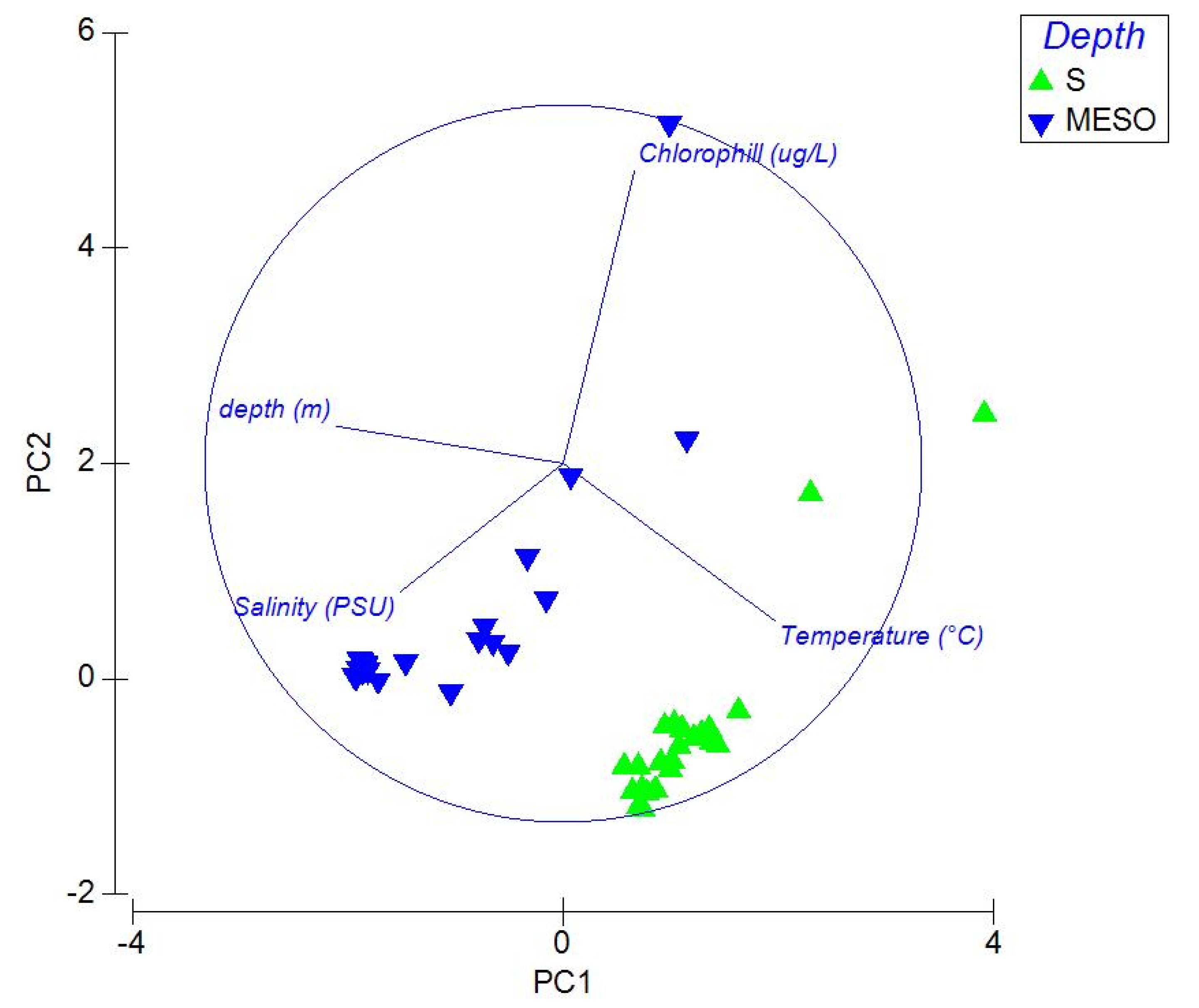
Principal Component Analysis (PCA) (Figure 4) established that the epipelagic community was more correlated with temperature and salinity and the mesopelagic community was more correlated with salinity and depth.
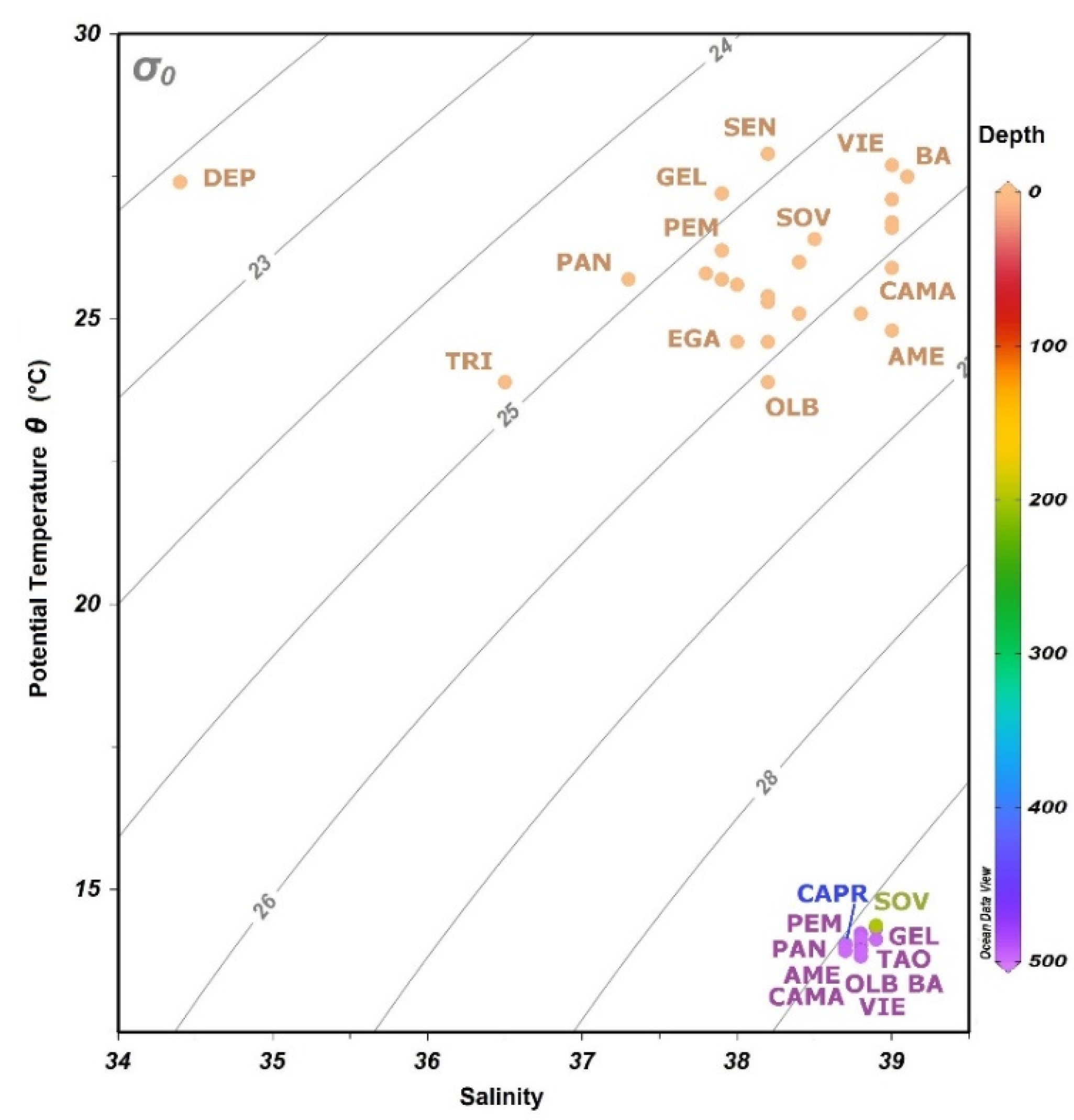
T-S diagram (Figure 5) shows how different surface water masses can be recognized as separated from a single deep one. Mesopelagic layer stations resulted very close each other, sometimes overlapping, while the epipelagic layer stations showed a wider difference in salinity and potential temperature. Finally, the T-S diagram also shows that the selected depth range (200–500 m below the sea level) for mesopelagic samples is correct.
3.1.3. Cruises 2013 and 2015
As regards the temperature of the 2013 cruise, surface waters were generally warmer than the deep ones. All the surface values oscillated between 18.5 and 21.4 °C with the maximum at station 07 (Montenegro shelf), but six stations of the Albanian coast showed a temperature below 18.0 °C (minimum 15.7 °C, at station Rre). All the deep points showed temperatures lower than those of the corresponding surface water, ranging from 12.3 (station 02, −121 m) to 16.0 °C (station GVL, −23 m). The widest variation between surface and bottom temperatures was recorded at station Tre (20.2–12.6 °C) in a water column of 79 m. Minimum ranges between surface and bottom were recorded along the southern Albanian coast (stations Kar, Par, Rre, Gra) with less than 1.6 °C difference, even in a water column of 233 m (Supplementary Material Table S4).
Relatively low salinity values (less than 38) were measured only in surface waters, with a minimum of two areas, one north of the Gargano promontory (37.5–37.6) and one in front of Montenegro coast (four stations all showing a surface salinity of 31.1–34.3). In all 39 stations of the 2013 cruise, the salinity measured at the deep collection points was higher than every corresponding surface value, and ranged from 38.6 (station Tre, −79 m) to 39.0 (station Ere, −88 m) (Supplementary Material Table S4).
During the 2015 cruise, the range of temperature in surface waters (11.5–15.9 °C) was wider than that of the deep ones (12.8–15.8 °C). The maximum surface temperature was measured at station Kar3, and the minimum at station PnG. In general, the Balkan side of the basin was warmer than the Italian side. The maximum deep temperature was measured at station Kar2 (15.8 °C, at −224 m), and the minimum at PnG (12.7 °C at −61 m). Additionally, in the deep waters, the Italian side of the basin appeared colder than the Balkan one. The maximum variation between surface and bottom temperatures was recorded at station Otr (11.5–14.1 °C) in a water column of 83 m. Minimum differences between surface and bottom were recorded along the central part of the basin with a difference of 0.04 °C even in a water column of 255 m at station 13 (Supplementary Material Table S5).
Relatively low salinity values (less than 38) were measured only in surface waters of the Italian side of the Otranto Channel, with minimum (36.3) at station PnG. In all 25 stations of this cruise, the salinity measured at the deep collection points was higher than every corresponding surface value and ranged from 37.6 (station PnG, −61 m) to 38.9 (station Kar2, −224 m) (Supplementary Material Table S5).
3.2. Taxonomic Composition of Samples
3.2.1. Cruise 2017
Dinophyta and Ciliophora were classified according to 60 genera (33 and 27, respectively) (Table S3). Total microplankton abundances were not homogeneous; the highest abundance was found in the deep sample (32 m depth) of the Po river delta station (DEP) with 1268 ind L−1. The poorest sample in terms of abundance was the deep sample (500 m depth) of station NAP with 0.1 ind L−1 in total.
Differences between epipelagic and mesopelagic samples in terms of total abundances are shown in Figure 6. The epipelagic community had more heterogeneity in space, with lowest abundance values in Thyrrenian Sea and the highest in the north of the Adriatic Sea. Contrarily, the mesopelagic community (200–500 m depth) was more homogeneous in terms of abundances.
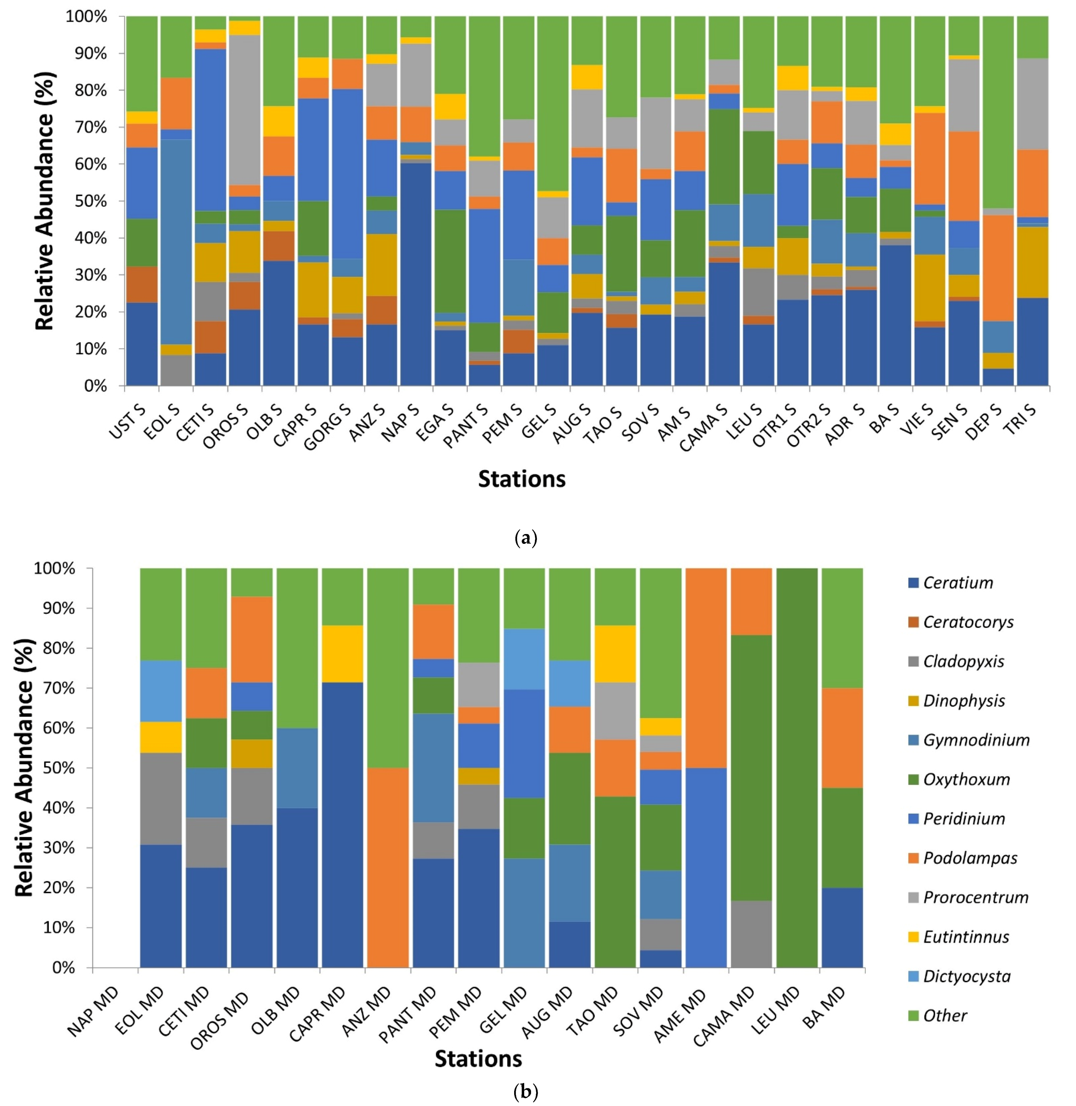
From relative abundances, a histogram representing the epipelagic assemblages of the 10 most important species found (Figure 7) that they were almost the same for epipelagic and mesopelagic layers, except for Dictyocysta and Ceratocorys. Ceratium was always present with variable percentages, except for at the EOL station in which Gymnodinium had the higher relative abundance. Peridinium had higher relative abundance in the Thyrrenian Sea (except for EOL, OROS and OLB), decreasing towards the Ionian and northward Adriatic Sea.
Regarding mesopelagic samples, Ceratium was always present in the Thyrrenian Sea (except for ANZ and NAP) and in the BA Adriatic station, while it was rare or absent in the south of Italy. Gymnodinium, contrary to the epipelagic layer, had the higher relative abundances in the mesopelagos of southern Italy. The presence of Peridinium was more heterogeneous than in the epipelagic samples. Oxythoxum had higher relative abundances in the south of Italy, except for PEM and AME. Prorocentrum was present in almost all stations of the epipelagic layer and only in three stations of the mesopelagic one. Podolampas, on the contrary, was present in almost all surfaces and deep stations.
Dinophyta were generally more abundant than Ciliophora. Gymnodinium and Ceratium were the most abundant genera, with averages of 29.35 ± 2.6 SE ind L−1 and 9.73 ± 24.4 ind L−1, respectively.
Among Ciliophora, the most abundant genus was Amphorellopsis, even if it is present only in three stations (maximum abundance in DEP S station). Without considering the deep North Adriatic stations (where the maximum water column was 33 m), Ciliophora and Dinophyta were more abundant in surface waters (average, 31.14 ± 18.93 ind L−1) than in deep ones (4.49 ± 1.07 ind L−1).
From SIMPER analysis, species contribution was observed. For the epipelagic community, Ceratium was the main genus (mainly represented by the species C. furca) (31.40% of contribution), followed by Peridinium (14.41%, Supplementary Material Figure S1). For the mesopelagic community Ceratium and Oxythoxum were the main components, with 30.41% and 20.91% of contribution, respectively (Figure 7).
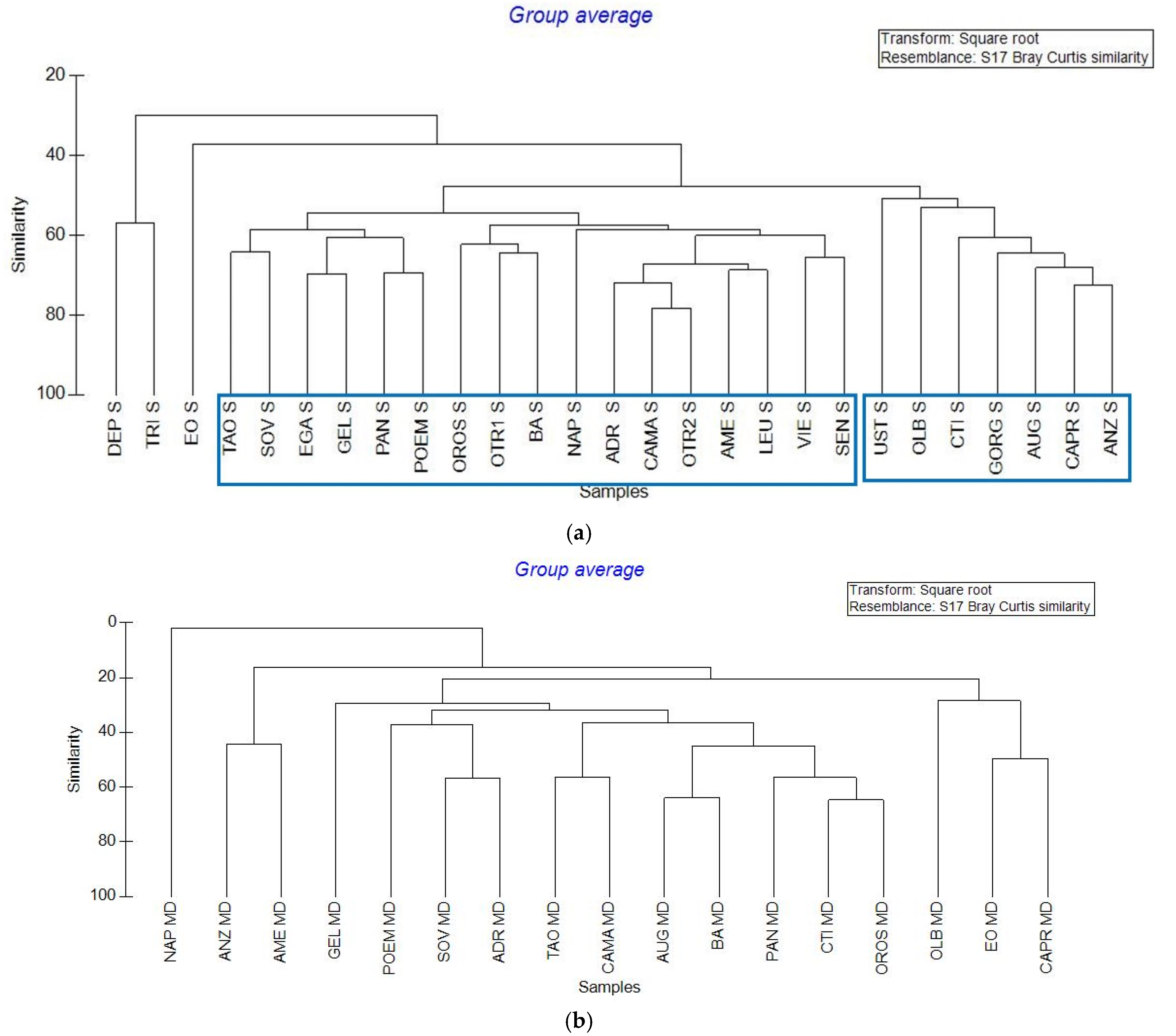
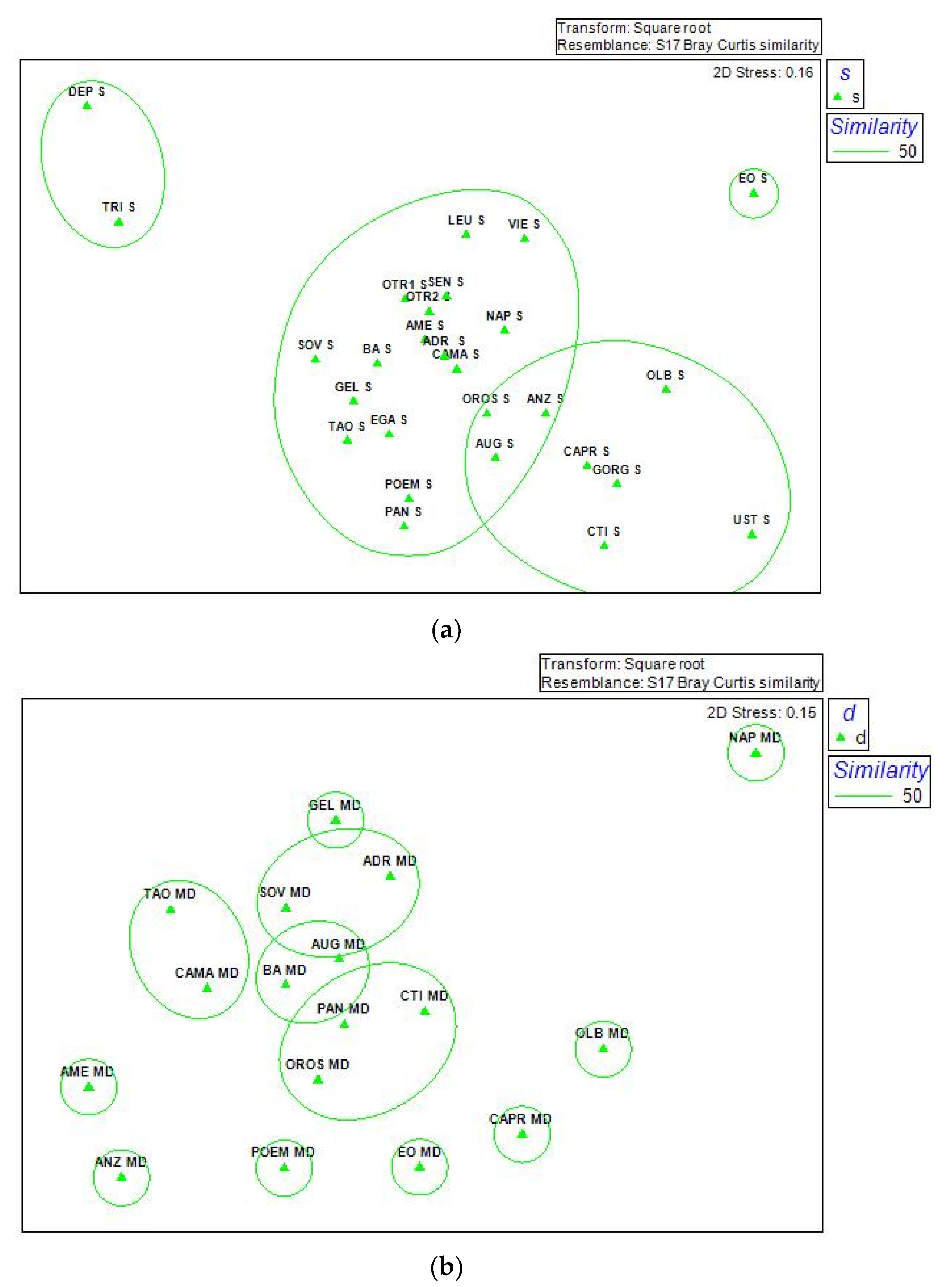
Hierarchical Cluster analysis (Figure 8) was performed dividing epipelagic and mesopelagic samples. In epipelagic cluster at 50% of similarity were recognizable in two major groups (two blue rectangles in Figure 8). Roughly, these two groups individuate one area corresponding to the Tyrrhenian Sea (six stations grouped together, plus AUG in the Ionian Sea) and another one corresponding to the “non Tyrrhenian” sea (10 stations in the Ionian Sea, plus NAP, OROS, VIE, SEN, BA, OLB, UST in other seas). The two stations of the North Adriatic (DEP, and TRI) represented a third group. The EOL station remained isolated. Samples collected in the mesopelagic layer (between 200 and 500 m below the sea level) were more scattered, grouping only at smaller similarities. These results were highlighted by the n-MDS analysis (Figure 9) in which epipelagic samples were grouped better than mesopelagic ones at 50% similarity.
3.2.2. Cruises 2013 and 2015
An analysis of samples collected in 2013 and 2015, only in the Southern Adriatic Sea, allowed us to examine this geographic area in detail, in different seasons, with results based on a total of 38 taxa (genera).
In 2013, 12 genera of Dinophyta and 26 of Ciliophora were identified, on a total of 39 epipelagic (surface), and 15 mesopelagic (depth, more than 200 m) samples. The sample with the highest abundance was the surface sample of station Tre (370.3 ind L−1) while in station 21, in the Otranto Channel, the surface sample presented the lowest abundance (0.3 ind L−1). Dinophyta (average, in epipelagic samples 3.23 ± 1.21 ind L−1 and 0.89 ± 0.58 ind L−1 in mesopelagic) were more abundant than Ciliophora (average, in epipelagic samples 0.19 ± 0.11 ind L−1 and 0.18 ± 0.16 ind L−1 in mesopelagic) although they were represented by a smaller number of genera. Ceratium was the most abundant genus with an average of 16.84 ± 3.57 ind L−1. The most abundant genus of Ciliphora was Stenosemella with an average abundance of 1.62 ± 1.55 ind L−1.
In 2015, 29 genera (8 Dinophyta and 21 Ciliophora) were identified on a total of 24 epipelagic and 13 mesopelagic samples. The highest abundance was found in the epipelagic sample in Pennagrossa (PnG) with 348.5 ind L−1. The station with lowest abundance was Karaburun 3 (Kar3) with 0.5 ind L−1. The genera with higher abundance were Ceratium (average, 18.73 ± 6.18 ind L−1) for Dinophyta and Codonellopsis (average, 1.94 ± 1.14 ind L−1) for Ciliophora.
3.2.3. Comparison between 2013, 2015 and 2017
Taking into account only samples collected in the South Adriatic Sea (from LEU to BA) in 2017, it was possible to compare data between the three years, considering for the mesopelagic layer only samples collected at more than 200 m of depth. The total genera found in all three cruises (in the considered area) was 52. Here, samples were renamed with the addition of S for epipelagic (surface) or MD for mesopelagic (maximum depth) samples, and also considering the year (2013, 2015, 2017).
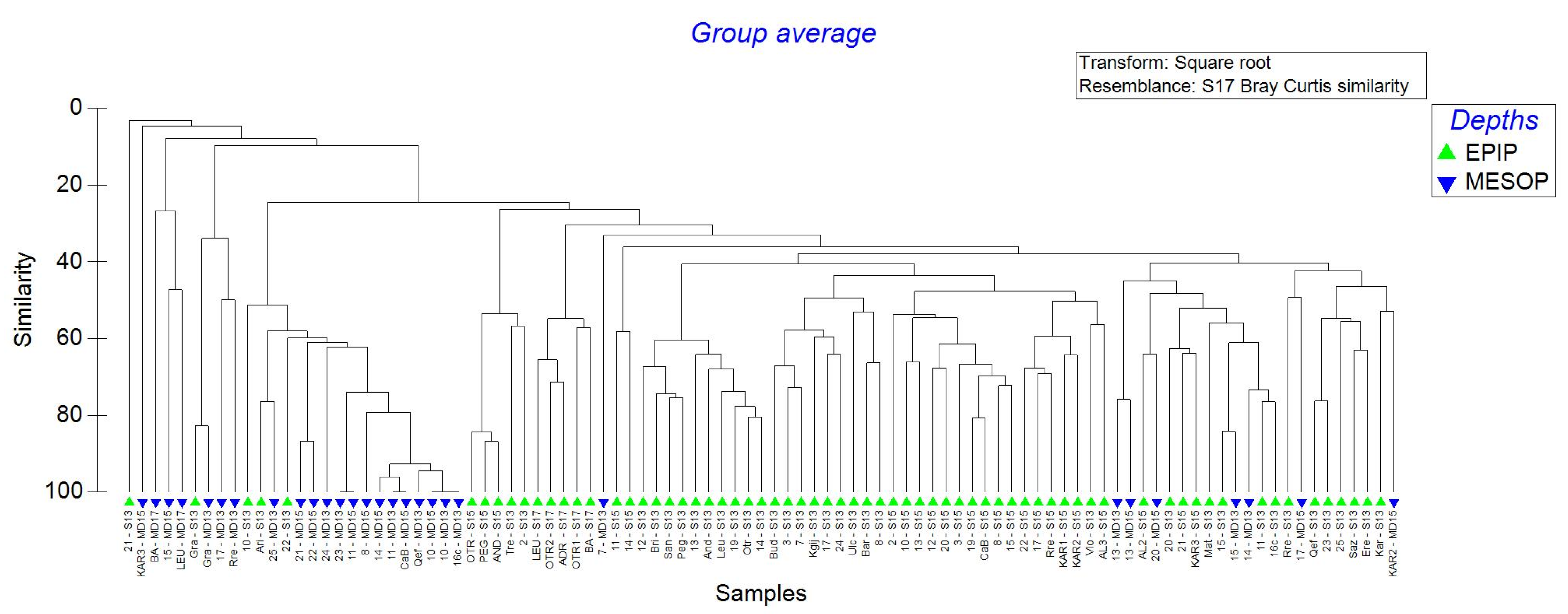
The Hierarchical analysis (Figure 10) showed an evident separation between epipelagic and mesopelagic samples, independent from the year. Even considering a very low level of similarity (30%, which includes 63 of the 68 epipelagic samples) the mesopelagic samples did not form large groups. However, mesopelagic samples belonging to the NE Southern Adriatic from years 2013 and 2015 (10—MD13 and 10—MD15) showed 100% similarity together with the SE Southern Adriatic from year 2013 (16c—MD13). Additionally, two mesopelagic groups, one with two samples belonging to Canyon Bari locality of 2015 collection (CaB—MD15) and Central Southern Adriatic of 2013 collection (11—MD13) and the other one from Central Southern Adriatic of 2015 (11—MD15) and NE Ionian from 2013 collection (23—MD13) had 100% of similarity. Samples belonging to Otranto Channel (21—MD13) and Karaburun 3 (Kar3—MD15) were very isolated with 3.25% and 4.65% similarity with other samples, respectively.
Notwithstanding the restricted geographic area (South Adriatic Sea), the statistical grouping of surface stations allowed one to recognize distinct assemblages of microplankton. In detail, the narrower point of the basin, corresponding to the Otranto Channel (width, about 40 NM) clearly showed the presence of three distinct microplankton communities, one on each side of the basin, and one in the middle (Figure 10, surface points 2013–2015).
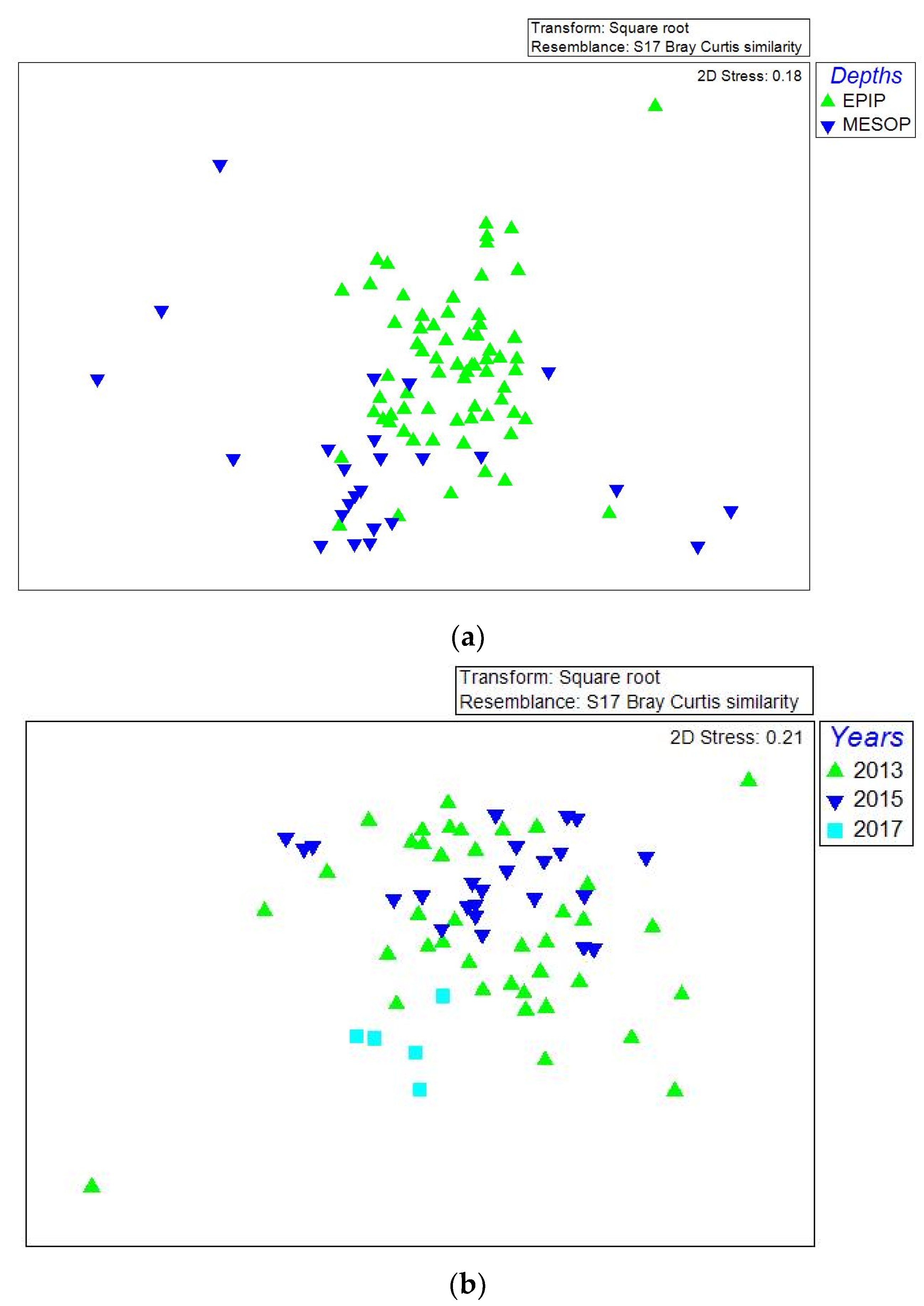
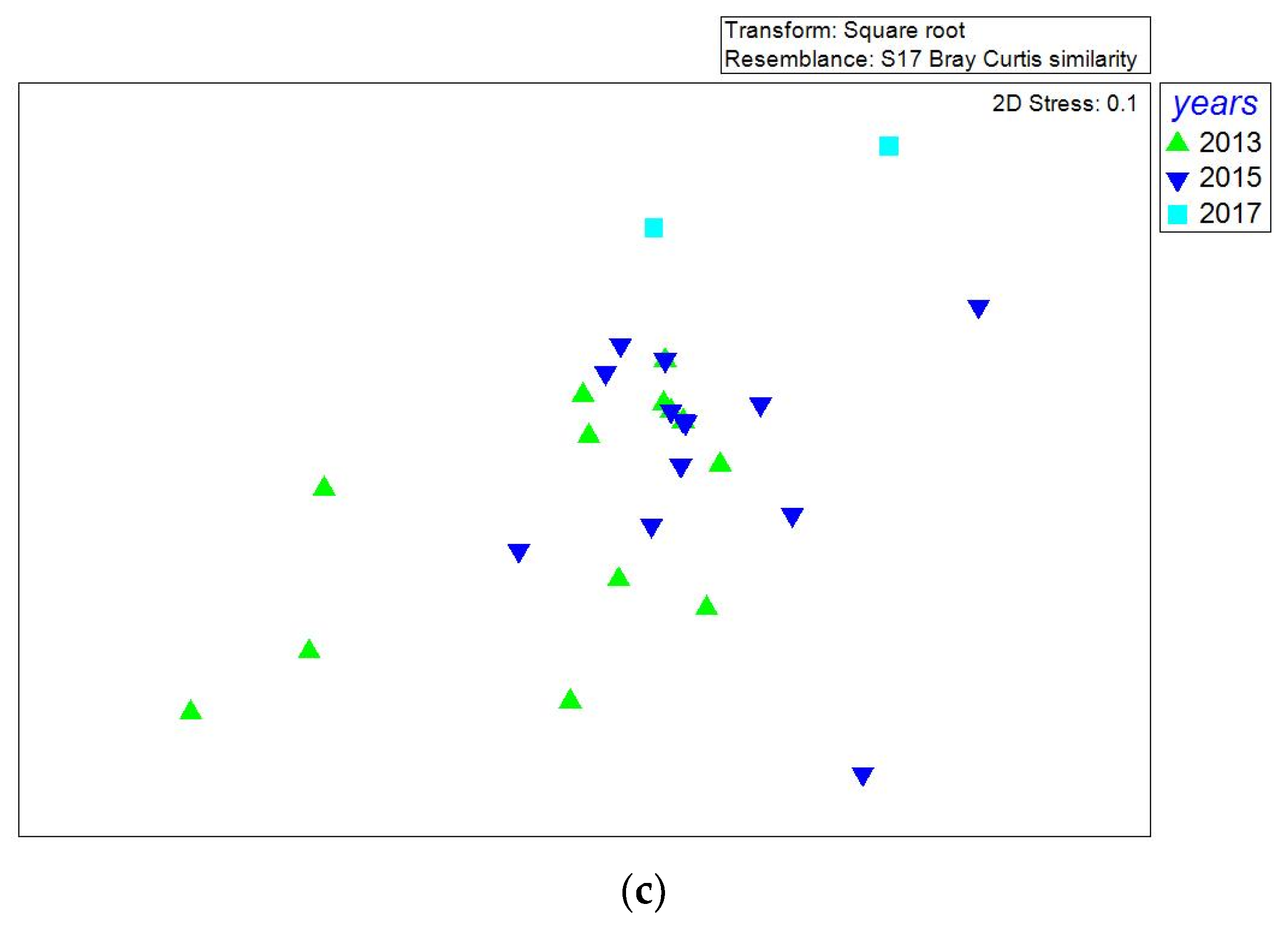
The n-MDS analysis showed that epipelagic samples from the three years grouped together, whereas the mesopelagic samples were more scattered and isolated (Figure 11a). Additionally, it is to note that most samples from 2013–15 grouped both at epi- and mesopelagic depths (Figure 11b,c), but only epipelagic samples from 2017 grouped with some previous (2013 and 2015) samples.
4. Discussion
The present study stems from a couple of oceanographic cruises carried out in the South Adriatic Sea in 2013 and 2015 where distinct assemblages of taxa were recognized in the surface microplankton (for 2013 data, see [25]). Data deriving from deep sea samples were not analyzed in that study because their surprising differences were interpreted as someway affected by the sample collection. In fact, deep samples were collected close (3–5 m) to the bottom at very different depths (23–1168 m below the sea level), thus suggesting the diversification found in deep microplankton composition as linked to the variability of the benthic environment, at different depths. Data from literature related to single stations over long time periods [21,22,24,30], although not referable to geographic differences, also report a more variable composition of deep microplankton when compared with the surface one at the same collection station. These results appear as contradictory if opposed to the stability of conditions (e.g., darkness, temperature, salinity) which are unaltered by space and time at those depths. Already in [15], the diversification of microplankton appeared as not justified by the variability of conditions and the authors alerted us to the importance of avoiding considering microplankton diversity patterns as affected by those geographical cues, which seem to affect metazoan distribution in the oceans.
Analyzing samples belonging from 2017 allowed us to have more information about Dinophyta and Ciliophora assemblages and how they are distributed in a large geographic area. We found differences between epipelagic and mesopelagic layers. The deep collections were performed at a closer depth interval (200–500 m) and mostly far from the bottom, to minimize possible interferences upon the final similarity of samples. Analysis allowed us to better specify that the taxa assemblages recognized in the epipelagic waters were different from those in mesopelagic ones at more than 200 m below the sea surface. This is not surprising because, at least for the autotrophic components (Phytoplankton), their reduction or even disappearance is obvious in the mesopelagic habitat and indeed from our analysis of abiotic factors, Chlorophyll a was the variable (together with depth) with the higher coefficient correlation with the studied communities. In addition, as resulted from the analysis, mesopelagic microplankton did not group together as the epipelagic microplankton did, showing a lack of similarity notwithstanding the higher homogeneity of the deep environment in terms of abiotic factors, as resulted from temperature and salinity maps and from the T-S diagram.
Consequently, we suggest caution in indicating environmental variables as drivers of the microplankton composition in the deep sea. Here, we propose lacking evidence of the correlation between water mass and microplankton homogeneity. The spatial variability of mesopelagic microplankton (within a homogeneous environment) could be related with the large geographic scale of species distribution which determines a reduced connectivity [18,19] and assemblages regulated by chance and not by environment constraints. It is time to verify if this conceptual frame can also include the distribution of unicellular organisms in the open sea, and/or the space scale on which it works (if similar or different from other plankton size categories), but also go further in studying the trend of the deep communities through seasons and years to strengthen our theory.
Although some environmental data are lacking (as those on currents and water mass circulation), we cannot ignore that scientific literature considers the mesopelagic zone as more stable than the epipelagic layer. In presence of environmental homogeneity of mesopelagos, the biotic variables (the taxa) assume the role of diversity elements.
Finally, the high spatial diversification of mesopelagic microplankton allowed us to re-consider the interpretation of the results of the sample collection of 2013, when the high diversification of deep samples was not considered by [25] because of the proximity to the bottom at very different depths where the samples were collected. Here, with most of the mesopelagic samples collected in a narrower depth range, and far from the bottom, we can suggest the deep community isolation (the lacking of connectivity) as co-responsible (if not the main responsible element) for the weak similarity between deep communities both in large (Central Mediterranean) and in restricted (the South Adriatic) geographic areas [31].
Supplementary Materials
The following are available online at www.mdpi.com/xxx/s1.Table S1: Location of the 27 stations where the collection of microplankton was carried out in summer 2017. In each station are also indicated the two depths where the samples have been collected (S: surface, MD: maximum depth) and the water volume (L) filtered for each sample, and the abiotic parameters obtained from a multiparametric probe: Temperature (°C), Salinity and Clorophyll a (μg L−1); Table S2: Location of the 39 stations interested by collection of microplankton in spring 2013; Table S3: Location of the 24 stations interested by collection of microplankton in winter 2015. In each station it is indicated the depth (m) where the samples have been collected (at Surface, Surf, and maximum depth, Deep), and the total volume (L) of water filtered per sample; Table S4: Water characteristics at surface (3 m) and bottom (different depths) of 39 stations, for the collection of microplankton samples in South Adriatic Sea. Period of collection: 09–18 May 2013; Table S5: Water characteristics at surface (2–3 m) and bottom (different depths) of 24 stations for the collection of microplankton samples in South Adriatic Sea. Period of collection: 3–13 March 2015; Table S6: SIMPER analysis results. Above, taxa contribution of epipelagic community; below, taxa contribution of mesopelagic community; Table S7: Presence/abundance (ind L−1) of microplankton taxa, collected in 27 stations of Italian Seas, at 2 different depths (see Table 1), July 2017.
Author Contributions
Conceptualization, G.B., L.G.; methodology, G.B., L.Y.; formal analysis, J.V., S.M., A.G.; writing—original draft preparation, J.V., G.B., L.Y., L.G.; writing—review and editing, all authors.; funding acquisition, G.B., L.G., L.Y. All authors have read and agreed to the published version of the manuscript.
Funding
Samples of 2013 and 2015 have been collected in the frame of the EU FS7 “CoCoNET” project (Coordinator, F. Boero). The 2017, samples were linked in the frame of the oceanographic expedition MSFD-IT-3-2017 as part of the EU Marine Strategy Framework Directive 2008/56/EC (MSFD). V.J. was supported by an Erasmus+ Fellowship at IEO, Centro Oceanográfico de Málaga, Instituto Español de Oceanografía, 29640 Fuengirola, Spain.
Institutional Review Board Statement
Not applicable.
Informed Consent Statement
Not applicable.
Data Availability Statement
The data presented in this study are available as supplementary material in https://www.mdpi.com/article/10.3390/w13091263/s1.
Acknowledgments
Authors want to thank the crews of the “Urania”, and “Minerva 1” Research vessels, and, especially, Pino Arena for sampling execution during the 2017 cruise. All of the authors are also grateful for the deep and rich discussion stimulated by the reviewers, which greatly ameliorated the manuscript.
Conflicts of Interest
The authors declare no conflict of interest.
References
- Stoecker, D.K.; Gustafson, D.E.; Verity, P.G. Micro- and meso-protozooplankton at 140° W in the equatorial pacific. Heterotrophs and mixotrophs. Aquat. Microb. Ecol. 1996, 10, 273–282. [Google Scholar] [CrossRef]
- Moscatello, S.; Rubino, F.; Saracino, O.D.; Belmonte, G.; Boero, F. Plankton biodiversity around the Salento Pensinsula (South East Italy): An integrated water/sediment approach. Sci. Mar. 2004, 68, 85–102. [Google Scholar]
- Rubino, F.; Saracino, O.D.; Moscatello, S.; Belmonte, G. An integrated water/sediment approach to study plankton (a case study in the southern Adriatic Sea). J. Mar. Syst. 2009, 78, 536–546. [Google Scholar] [CrossRef]
- Lennon, J.T.; Jones, S.E. Microbial seed banks: The ecological and evolutionary implications of dormancy. Nat. Rev. Microbiol. 2011, 9, 119–130. [Google Scholar] [CrossRef]
- Fenchel, T. There are more small than large species? Oikos 1993, 68, 375–378. [Google Scholar] [CrossRef]
- Finlay, B.J. Global dispersal of free-living microbial eukaryote species. Science 2002, 296, 1061–1063. [Google Scholar] [CrossRef] [Green Version]
- Dale, B. Dinoflagellate resting cysts: Benthic plankton. In Survival Strategies of the Algae; Frixell, G.A., Ed.; Cambridge University Press: Cambridge, UK, 1983; pp. 69–136. [Google Scholar]
- Taylor, F.J.R. General group characteristics; special features of interest; short history of dinoflagellates study. In The Biology of Dinoflagellates; Taylor, F.J.R., Ed.; Botanical Monographs, University of California Press: Berkeley, LA, USA, 1987; Volume 21, pp. 1–23. [Google Scholar]
- Paranjape, M. Occurrence and significance of resting cysts in a hyaline tintinnid Helicostomella subulata (Ehre.) Jorgensen. J. Exp. Mar. Biol. Ecol. 1980, 48, 23–33. [Google Scholar] [CrossRef]
- Kim, Y.-O.; Suzuki, T.; Taniguchi, A. A new species in the genus Cyrtostrombidium (Ciliophora, Oligotrichia, Oligotrichida): Its morphology, seasonal cycle and resting stage. J. Eukaryot. Microbiol. 2002, 49, 338–343. [Google Scholar] [CrossRef]
- Montagnes, D.J.S.; Wilson, D.; Brooks, S.J.; Lowe, C.; Campey, M. Cyclical behaviour of the tide-pool ciliate Strombidium oculatum. Aquat. Microb. Ecol. 2002, 28, 55–68. [Google Scholar] [CrossRef] [Green Version]
- Belmonte, G.; Rubino, F. Resting cysts from coastal marine plankton. Oceanogr. Mar. Biol. Annu. Rev. 2019, 57, 1–88. [Google Scholar]
- Stoecker, D.K.; Davis, L.H.; Anderson, D.M. Fine scale spatial correlations between planktonic ciliates and dinoflagellates. J. Plankton Res. 1984, 6, 829–842. [Google Scholar] [CrossRef]
- Briggs, J.C.; Bowen, B.W. A realignment of marine biogeographic provinces with particular reference to fish distributions. J. Biogeogr. 2012, 39, 12–30. [Google Scholar] [CrossRef]
- Moss, J.A.; Henriksson, N.L.; Pakulski, J.D.; Snyder, R.A.; Jeffrey, W.H. Oceanic Microplankton do not adhere to the latitudinal diversity gradient. Microb. Ecol. 2020, 79, 511–515. [Google Scholar] [CrossRef] [PubMed]
- Barton, A.D.; Pershing, A.J.; Litchman, E.; Record, N.R.; Edwards, K.F.; Finkel, Z.V.; Kiørboe, T.; Ward, B.A. The biogeography of marine plankton traits. Ecol. Lett. 2013, 16, 522–534. [Google Scholar] [CrossRef]
- Calbet, A.; Landry, M.R. Phytoplankton growth, microzooplankton grazing, and carbon cycling in marine systems. Limnol. Oceanogr. 2004, 49, 51–57. [Google Scholar] [CrossRef] [Green Version]
- Rosenzweig, M.L. Species Diversity in Space and Time; Cambridge University Press: Cambridge, UK, 1995; 436p. [Google Scholar]
- Belmonte, G. Species richness in isolated environments. The disregarded role of time. J. Biodivers. 2012, 3, 273–280. [Google Scholar]
- McManus, M.A.; Woodson, C.B. Plankton distribution and ocean dispersal. J. Exp. Biol. 2012, 215, 1008–1016. [Google Scholar] [CrossRef] [Green Version]
- Modigh, M.; Castaldo, S. Variability and persistence in tintinnid assemblages at a Mediterranean coastal site. Aquat. Microb. Ecol. 2002, 28, 299–311. [Google Scholar] [CrossRef] [Green Version]
- Gómez, F.; Gorsky, G. Annual microplankton cycles in Villefranche Bay, Ligurian Sea, NW Mediterranean. J. Plankton Res. 2003, 25, 323–339. [Google Scholar] [CrossRef]
- Sitran, R.; Bergamasco, A.; Decembrini, F.; Guglielmo, L. Temporal succession of tintinnids in the northern Ionian Sea, Central Mediterranean. J. Plankton Res. 2007, 29, 495–508. [Google Scholar] [CrossRef]
- Hsu, K.J.; Montadert, L.; Bernoulli, D.; Cita, M.B.; Erickson, A.; Garrison, R.E.; Kidd, R.B.; Melieres, F.; Muller, C.; Wright, R. History of the Mediterranean salinity crisis. Nature 1977, 267, 399–403. [Google Scholar] [CrossRef]
- Moscatello, S.; Belmonte, G.; Guglielmo, L.; Hajderi, E. Microzooplankton in The South Adriatic Sea. In Proceedings of the 41st CIESM Congress, Kiel, Germany, 12–16 September 2016; Volume 41, p. 484. [Google Scholar]
- Pierce, R.W.; Turner, J.T. Global biogeography of marine tintinnids. Mar. Ecol. Prog. Ser. 1993, 94, 11–26. [Google Scholar] [CrossRef]
- Terlizzi, A.; Anderson, M.J.; Bevilacqua, S.; Ugland, K.I. Species-accumulation curves and taxonomic surrogates: An integrated approach for estimation of regional species richness. Divers. Distrib. 2014, 20, 356–368. [Google Scholar] [CrossRef]
- Clarke, K.R.; Warwick, R.M. Similarity-based testing for community pattern: The 2-way layout with no replication. Mar. Biol. 1994, 118, 167–176. [Google Scholar] [CrossRef]
- Schlitzer, R. Ocean Data View. 2018. Available online: https://odv.awi.de (accessed on 15 April 2021).
- Sitran, R.; Bergamasco, A.; Decembrini, F.; Guglielmo, L. Microzooplankton (tintinnid ciliates) diversity: Coastal community structure and driving mechanisms in the southern Tyrrhenian Sea (Western Mediterranean). J. Plankton Res. 2009, 31, 153–170. [Google Scholar] [CrossRef] [Green Version]
- Umani, S.F.; Monti, M.; Minutoli, R.; Guglielmo, L. Recent advances in the Mediterranean researches on zooplankton: From spatial-temporal patterns of distribution to processes oriented studies. Adv. Oceanogr. Limnol. 2010, 1, 295–356. [Google Scholar] [CrossRef]
Figure 1.
(a) Map of the study area showing the location, 27 sampling stations in the Italian Seas (2017); and maps of the South Adriatic where two cruises were carried out in 2013 (39 stations) (b), and 2015 (24 stations) (c).
Figure 1.
(a) Map of the study area showing the location, 27 sampling stations in the Italian Seas (2017); and maps of the South Adriatic where two cruises were carried out in 2013 (39 stations) (b), and 2015 (24 stations) (c).

Figure 2.
Map of the study area showing differences in temperature (°C) of (a) epipelagic and (b) mesopelagic stations.
Figure 2.
Map of the study area showing differences in temperature (°C) of (a) epipelagic and (b) mesopelagic stations.

Figure 3.
Map of the study area showing differences in salinity of (a) epipelagic and (b) mesopelagic stations.
Figure 3.
Map of the study area showing differences in salinity of (a) epipelagic and (b) mesopelagic stations.

Figure 4.
Principal Component Analysis (PCA) on abiotic data and taxa.

Figure 5.
T-S diagram of superficial and deep stations. Color bar shows the depths (m). Not all stations have been indicated at each group (epipelagic and mesopelagic).
Figure 5.
T-S diagram of superficial and deep stations. Color bar shows the depths (m). Not all stations have been indicated at each group (epipelagic and mesopelagic).

Figure 6.
Total microplankton abundance (ind L−1) at (a) epipelagic (2–4 m below the sea level), and (b) mesopelagic (200–500 m below the sea level) layers.
Figure 6.
Total microplankton abundance (ind L−1) at (a) epipelagic (2–4 m below the sea level), and (b) mesopelagic (200–500 m below the sea level) layers.

Figure 7.
Relative abundances (%) of the main 10 taxa identified in samples collected in 2017 divided by (a) Epipelagic (2–4 m below the sea level) and (b) Mesopelagic (200–500 m below the sea level) layers 2017. Remaining genera were grouped in Other.
Figure 7.
Relative abundances (%) of the main 10 taxa identified in samples collected in 2017 divided by (a) Epipelagic (2–4 m below the sea level) and (b) Mesopelagic (200–500 m below the sea level) layers 2017. Remaining genera were grouped in Other.

Figure 8.
Cruise 2017. Representation of hierarchical cluster. (a) Epipelagic (surface) samples from 27 stations; (b) Mesopelagic (200–500 m) samples from 17 stations.
Figure 8.
Cruise 2017. Representation of hierarchical cluster. (a) Epipelagic (surface) samples from 27 stations; (b) Mesopelagic (200–500 m) samples from 17 stations.

Figure 9.
Cruise 2017. Representation of non-parametric Multidimensional Scaling (nMDS) of (a) epipelagic sample (s), 27 stations (2–4 m below the sea level), and (b) mesopelagic samples (d) (200–500 m below the sea level), from 17 stations.
Figure 9.
Cruise 2017. Representation of non-parametric Multidimensional Scaling (nMDS) of (a) epipelagic sample (s), 27 stations (2–4 m below the sea level), and (b) mesopelagic samples (d) (200–500 m below the sea level), from 17 stations.

Figure 10.
Representation of Hierarchical cluster analysis of samples collected in 2013, 2015 and 2017, only in Southern Adriatic Sea (Dinophyta and Ciliophora genera considered). For MD (maximum depth) samples, only those at more than 200 m below the sea level have been considered.
Figure 10.
Representation of Hierarchical cluster analysis of samples collected in 2013, 2015 and 2017, only in Southern Adriatic Sea (Dinophyta and Ciliophora genera considered). For MD (maximum depth) samples, only those at more than 200 m below the sea level have been considered.

Figure 11.
Representation of non-parametric multidimensional scaling (nMDS) of Southern Adriatic Sea samples (Dinophyta and Ciliophora genera considered) collected in 2013, 2015, and 2017, including (a) epipelagic and mesopelagic samples together, (b) only epipelagic samples and (c) only mesopelagic samples. For MD (maximum depth) samples, only those at more than 200 m below the sea level, have been considered.


Table 1.
Results of BEST test.
| Variables | 1 Depth (m) 2 Temperature (°C) 3 Salinity (psu) 4 Chl a (µg L−1) | |
|---|---|---|
| No. Vars | Corr. | Selections |
| 2 | 0.575 | 1; 4 |
| 1 | 0.574 | 1 |
| 3 | 0.554 | 1; 2; 4 |
| 2 | 0.512 | 1; 2 |
| 4 | 0.494 | All |
| 3 | 0.484 | 1; 3; 4 |
| 2 | 0.461 | 1; 3 |
| 3 | 0.454 | 1–3 |
| 2 | 0.385 | 2; 4 |
| 3 | 0.315 | 2–4 |
Publisher’s Note: MDPI stays neutral with regard to jurisdictional claims in published maps and institutional affiliations. |
© 2021 by the authors. Licensee MDPI, Basel, Switzerland. This article is an open access article distributed under the terms and conditions of the Creative Commons Attribution (CC BY) license (https://creativecommons.org/licenses/by/4.0/).
Share and Cite
MDPI and ACS Style
Vannini, J.; Yebra, L.; Granata, A.; Guglielmo, L.; Moscatello, S.; Belmonte, G. Horizontal Distribution of Deep Sea Microplankton: A New Point of View for Marine Biogeography. Water 2021, 13, 1263. https://doi.org/10.3390/w13091263
AMA Style
Vannini J, Yebra L, Granata A, Guglielmo L, Moscatello S, Belmonte G. Horizontal Distribution of Deep Sea Microplankton: A New Point of View for Marine Biogeography. Water. 2021; 13(9):1263. https://doi.org/10.3390/w13091263
Chicago/Turabian StyleVannini, Jessica, Lidia Yebra, Antonia Granata, Letterio Guglielmo, Salvatore Moscatello, and Genuario Belmonte. 2021. "Horizontal Distribution of Deep Sea Microplankton: A New Point of View for Marine Biogeography" Water 13, no. 9: 1263. https://doi.org/10.3390/w13091263
Note that from the first issue of 2016, this journal uses article numbers instead of page numbers. See further details here.