
Applying Optimization to Support Adaptive Water Management of Rivers


1
Department of Computational Landscape Ecology, Helmholtz-Centre for Environmental Research—UFZ, 04318 Leipzig, Germany
2
IHCantabria—Instituto de Hidráulica Ambiental, Universidad de Cantabria, 39011 Santander, Spain
*
Author to whom correspondence should be addressed.
Water 2021, 13(9), 1281; https://doi.org/10.3390/w13091281
Submission received: 29 March 2021
/
Revised: 28 April 2021
/
Accepted: 28 April 2021
/
Published: 30 April 2021
(This article belongs to the Special Issue Integrated Water Resource System Modeling to Support Sustainable Water Management)
Abstract
:Adaptive water management is a promising management paradigm for rivers that addresses the uncertainty of decision consequences. However, its implementation into current practice is still a challenge. An optimization assessment can be framed within the adaptive management cycle allowing the definition of environmental flows (e-flows) in a suitable format for decision making. In this study, we demonstrate its suitability to mediate the incorporation of e-flows into diversion management planning, fostering the realization of an adaptive management approach. We used the case study of the Pas River, Northern Spain, as the setting for the optimization of surface water diversion. We considered e-flow requirements for three key river biological groups to reflect conditions that promote ecological conservation. By drawing from hydrological scenarios (i.e., dry, normal, and wet), our assessment showed that the overall target water demand can be met, whereas the daily volume of water available for diversion was not constant throughout the year. These results suggest that current the decision making needs to consider the seasonal time frame as the reference temporal scale for objectives adjustment and monitoring. The approach can be transferred to other study areas and can inform decision makers that aim to engage with all the stages of the adaptive water management cycle.
1. Introduction
The concept of integrated water resource management (IWRM) embodies the willingness to account for the economic, social, and ecological implications of water management [1]. River regulation, such as damming, barrages, and river training, can affect both the sediment balance, inducing morphological changes, and the hydrological regime [2,3]. As a consequence, many of the current water management decisions for regulated rivers worldwide aim for the sustainable use of water resources to protect natural ecosystems [4]. However, the rapid decline in freshwater biodiversity urges for prompt practical actions such as environmental flow implementation [5,6]. The concept of environmental water regime or environmental flow (e-flow) was first announced during The Brisbane Declaration (2007) [7] and ever since it has defined “the quantity, timing, and quality of water flows required to sustain freshwater and estuarine ecosystems and the human livelihoods and well-being that depend on these ecosystems” [8,9,10,11].
In regulated rivers, sustainable use is typically achieved by management decisions controlling certain variables, such as consumption capping or water allocation, through downstream release for specific target ecological processes and/or components [12]. Regardless the management decision in question, the incorporation of e-flows into practice is fundamental to facilitating “the establishment of a water regime needed to manage rivers” [13] that acknowledge the importance of ecosystem needs [4]. Moreover, e-flow incorporation within management practices can also be associated with conservation and restoration objectives for targeted scales such as “passive” restoration approaches addressing the reduction of hydrological alteration stresses on biodiversity [14,15,16,17].
The complexity of the interactions characterizing our socio-ecosystems (sensu [18]) leads to difficulty in predicting the effects of certain factors (e.g., climate, water demand) that increase the uncertainty of results from specific water management actions [19]. This lack of security exacerbates the ongoing challenges for decision making in water management process, such as organizing efficient water governance systems [20], and leads to reduced capacity to resolve unexpected eventualities and future scenarios. The concept of “adaptive management”, as a fairly new paradigm for managing water resources in an integrated way, emerged in the last decades in response to the need to improve water management strategies [21,22]. This paradigm, which builds on the “learning-by-doing” approach, considers the improvement of management practices by learning from the outcomes of previously implemented management strategies [19,21]. Theoretically, this process consists of a constant loop of learning and adaptation between each adaptive water management cycle (AWMC) to achieve long-term management goals (e.g., restoration of hydrological conditions for endemic species). However, smaller adjustments based on shorter-term, ongoing outcomes could be made between each phase of the cycle (i.e., planning, doing, monitoring, and learning; see [21,23,24]). Practically, exact strategies to achieve adaptability within the AWMC are still lacking [25]—it calls for stronger links between management actions and subsequent monitoring strategies [17,23,26] to support the evidence of ecological improvement or degradation [26].
The adaptive management approach suits the challenge of incorporating e-flows into management (due to the uncertain nature of environmental outcomes after management decisions; [27,28]). The practical incorporation of e-flows into water management planning will require prompt adaptation of decisions and actions based on changing environmental conditions (e.g., hydrological, ecological, and climatic). The prediction of results from management actions under different scenarios (e.g., incorporating hydrological variability, climate change, and demand fluctuation) before their implementation represents a very powerful tool to anticipate consequences and reinforce the decision-making process to improve adaptability, sustainability, and ecosystem conservation. Overall, such a strategy will improve our ability to reveal management effects in complex systems as managed rivers [22].
E-flow incorporation into water management is often linked to the problem of balancing human and ecosystem water needs and maintaining ecosystem services provision when sustainable abstraction practices are sought. Different methods have been applied to support water management and water allocation in complex systems. Examples include economic approaches [29,30]; geographic information systems [31,32]; socio-hydrological and environmental assessments [33,34,35]; as well as a range of decision-support tools [36,37]. Usually, water management deals with a range of conflicting anthropogenic water-use objectives and, consequently, there are important trade-offs between water uses and demands [38]. The need for new instruments and frameworks that help decision-makers is still evident [28] and will increasingly put pressure on water managers dealing with future climate change effects [39,40]. Optimization is a decision support approach that has been applied for such water management problems at different scales, envisaging convoluted decision-making (among which there are trade-offs in river ecosystem services and river sediment budget maintenance; [2,41,42]) [43,44,45]. It enables the identification and evaluation of trade-offs and synergies among some management objectives (e.g., control of consumption, risk prevention, delivery of water for targeted species, hydropeaking control) before implementation takes place. The technical structure and features of the optimization approach (e.g., mathematical expression, multiple solutions) address many of the challenges (e.g., scenario analysis, real-world conditions representation) resulting from the need to incorporate e-flows into management planning [44]. Due to the absence of exact rules for the definition of e-flow requirements for rivers but rather distinct approaches [13,46,47], a series of strategies are possible to operationalize their incorporation within the optimization assessment (e.g., based on the consideration of natural-flow conditions or exploiting flow–biota correlations). A careful definition of e-flow requirements is hence needed to support the monitoring phase to enable the adaptive process [17,21].
In this paper, we developed an optimization assessment on the example of a targeted river basin in Northern Spain, which is providing water for an urban area of over 200,000 people. The specific objectives of the modeling exercise were (1) to demonstrate the suitability of a new methodology based on an optimization approach to mediate the incorporation of e-flows into the diversion management planning, (2) to discuss the challenges and limitations of the optimization model by drawing from the considered water management problem, and (3) to assess the potential of the optimization approach to foster adaptive management of water resources. We first present the conceptual framework underpinning the definition of the optimization assessment for water abstraction and the stages involved in the definition of the optimization problem for the selected case study (Section 2). The section also contains the description of the case study and the optimization problem incorporating environmental flows, as well as an illustration of the hydrological scenarios and the optimization modeling algorithm. Simulation results are presented in Section 3. Lastly, we discuss both the modeling assumptions and results, highlighting both the advantages and the disadvantages of the optimization assessment, and the implications for the diversion planning and river management providing suggestions for the best adoption of an adaptive process (Section 4).
2. Materials and Methods
2.1. The Optimization Framework
The optimization assessment framework presented in this study represents the “structured set of steps and considerations used for the formulation [of the optimization problem]” [44] underpinning the optimization modeling exercise conducted for the case study of the Pas River, Northern Spain (Section 2.2).
The stages of the optimization assessment framework that led to the definition of the optimization problem for the case study and their relationship to the AWMC phases (see Figure 1) are shown in Figure 2. As a first step, management objectives and water allocation decisions for the Pas River basin were assessed to understand the problem’s context and to identify priorities and water diversion practices (Section 2.2). This stage required the contextualization of the optimization problem to identify the best output information to be produced. In other words, a tailored result format was selected to enable the usage of information by the targeted user type (i.e., water managers and decision makers). Successively, based on the information identified during the contextualization phase, reference e-flow conditions were defined considering different biological groups present in the ecosystem (Section 2.3). For these biological groups, hydrological conditions (expressed as thresholds) were considered to preserve flow components from alterations caused by diversion. The “learning” process within the AWMC was based on the exploration of ecological effects from the management interventions [21]. As described in Section 2.3, given the exploratory nature of the assessment, the hydrological thresholds on the flow components (for each biological group) considered in this study were largely based on expert judgment. Lastly, information collected from the two previous stages was processed during the modeling stage, which considered the design of the optimization problem (e.g., solution approach) and its functions (i.e., objectives) both for the human water demand and for the considered biological groups (Section 2.4). Alongside the model development, hydrological scenarios reflecting daily mean discharge at the targeted location were developed and used as the reference (input) hydrological conditions for the optimization model runs (Section 2.6 and Section 2.5, respectively).
2.2. Case Study Area: The Pas River Basin
We used the Pas River basin in Northern Spain as the case study area for the optimization assessment development and application (Figure 3). The Pas River represents an ideal catchment to show the potential of optimization approaches to support adaptive water management planning. It subject to relatively strong human pressure, while it still provides a good representation of its potential natural condition. In this regard, most of its river water bodies show a good ecological status (sensu European Water Framework Directive; [48]) and provide habitats for iconic species for conservation such as Atlantic salmon. The Pas River system drains into the Cantabrian Sea (North–East Atlantic). Calcareous rock and sandstone formations dominate the basin which covers an area of 649 km2. The river network is defined by the three main rivers Pas, Pisueña, and Magdalena. The mean annual precipitation amounts to 1300 mm, and the mean annual daily flow (close to the river mouth) is 14 m3/s. Maximum flows are observed in April, and minimum discharges occur in September [49], close to the mouth. Water regulation in the basin is mainly implemented through surface water uptake by cross-channel weirs and pump injection into the water supply grid. A primary management objective is domestic water supply: water is mainly abstracted to satisfy the demand of the municipalities with annual volumetric allocation for the distinct municipalities. While there are no large infrastructures (e.g., dams) able to modify high flow and flood patterns, water diversion operations and water use can still influence the hydrological attributes related to low flows (e.g., magnitude of low flows, duration of droughts). Extended shoals and changes in the river flow as a consequence of traditional diversion practices represent a threat to ecosystems and freshwater biota. The ecological conditions of the aquatic ecosystem in the basin are monitored and defined by the Cantabrian Hydrological Confederation (CHC) which is also responsible for the drafting and development of the Basin Management Plans. In this study, we considered, as a setting for the optimization of water abstraction for municipal use, two distinct diversion points (i.e., DP1 and DP2)—as consumptive demand for the points we considered were 0.26 Hm3/year and 0.66 Hm3/year, respectively. Both points are not impacted by prior upstream flow diversion along the river network located on two distinct river segments (sensu [44]).
2.3. Definition of the e-Flow Requirements for the Pas River: Biological Groups and Hydrological Thresholds
The optimization of water diversion based on environmental needs requires the definition of reference hydrological conditions to ensure the conservation of key flow attributes (e.g., base flows, pulses) that support the ecosystem. Knowledge of the exact hydrological conditions for species and their cross-scale variation remain a core research gap in the field of freshwater biology [50]. Despite this gap, water management optimization assessment relies on flow–ecology relationship assumptions or eco-hydrological indicators (e.g., [51,52,53,54]) for the identification of optimal management strategies that facilitate the implementation of an adaptive management approach at appropriate scales [55]. E-flow requirements need to reflect hydrological conditions that support ecological processes and functions. A generalized optimization assessment approach considering a single taxonomic group (e.g., fish) can expose the risk of adverse effects on other components of the ecosystem and lead to unpredictable ecological results both at the short- and long-term scales [8,56]. Thus, the acknowledgment of the role of each biological group in the ecological framework is “fundamental to the maintenance of diverse and resilient communities into the future” [56]. In the frame of the study, despite not explicitly considering existing direct and indirect relationships among the considered biological groups, we simultaneously included the hydrological conditions of different biological groups to define the e-flow requirements in the Pas River throughout the year (Figure 4). In this regard, we encompassed three biological groups (Biological Group 1, 2, and 3) within the relevant levels of the trophic network of the ecosystems (from primary producers to apex predators). The process of e-flow requirement (R) definition (i.e., hydrological conditions for the biological groups) was based on the output of a workshop with a group of experts in the fields of hydrology, eco-hydrology, and freshwater biology from the IHCantabria (Santander, Spain). The e-flow requirements considered in this study are not absolute, meaning that they can be refined based on the dominant situation and idiosyncrasy of each watershed (establishing definitive values was out of the scope of this work). A summary of the requirements is shown in Table 1.
Biological Group 1 included fish species. Fish species are top predators and might represent an economic source for the local population in the region, associated with recreational angling [57]. Life cues of fish species are closely linked with the magnitude and timing of the distinct flow regimes. Despite different fish species have specific adaptation strategies and, hence, can tolerate the modification of either magnitude or timing of river flows to a certain extent, modification of flows during key stages of the lifecycle (e.g., migration, spawning, hatching, recruitment; [58,59,60,61,62]) could compromise population structure [63] or even increase the extinction risk [64,65]. The hydrological requirements (R1–R4) for Biological Group 1 aimed at the maintenance of certain flow conditions for cues (e.g., spawning or feeding) for the majority of the year (especially during dry periods) and at ensuring the occurrence of peak flows (e.g., for migration). Particularly related to the September period (characterized by reduced discharge), we exploited the synergy (and avoided algorithm conflicts) with R5 and R6 (described below) to ensure both survival and migration of the fish, which provided low flows and peak flows, respectively, during the month of September.
Biological Group 2 considered aquatic macroinvertebrates. The aquatic macroinvertebrates’ community composition was highly diverse (e.g., grazer, shredders, predators; [66]), and each community exhibits different responses to hydrological gradients and flow frequency [55,67,68]. Since additional experimental evidence is needed to define the accurate requirement of each taxonomic group, we considered the highest taxa occurrence probability (the underlying rationale was based on the Intermediate Disturbance Hypothesis [69]) as an indicator for the e-flow requirement for this group. The hydrological requirement (R5) for Biological Group 2 considered the occurrence of high flow conditions to reduce the alteration from flow diversion (e.g., flow magnitude and variability).
Biological Group 3, considered for the optimization assessment, refers to primary producers (PPs). PPs have a role in defining the presence of the other two groups (i.e., Biological Groups 1 and 2) because of their position at the base of the food-web [70]. PPs encompass a variety of taxonomic groups (from diatoms imbibed within the biofilm to macrophytes) that respond differently to changing hydrological patterns. The opportunistic response of PPs to variation in hydrological conditions defines the establishment of specific groups based on flow regime characteristics. We assumed that establishment success (i.e., ability to develop cover) was supported by a minimum flow during the dry period and, hence, defined the hydrological requirement (R6) in the targeted period (April–September).
2.4. Definition of the Pas River Optimization Problem
To identify the highest water supply sustainability in the river basin, the magnitude and timing of river water diversion operations need to be optimized to comply with the considered e-flow requirements. Hence, the latter generally constrains the availability of water for human consumption. Constrained multi-objective optimization is an optimization method based on the search for feasible solutions that directly limit the search space [71]. This method is frequently applied in real-world settings of structural and operational optimization assessments for water regulation assets [72,73]. An approach for constrained optimization is represented by the penalty-based approach; it allows transforming the problem into an “unconstrained” one—penalty (constraint) is incorporated into the objective function to reduce the fitness of the function based on the degree of the specified violation. The penalty-based approach particularly suits optimization assessments considering the high number of limiting conditions. Moreover, it can be easily implemented with evolutionary/genetic algorithms [74,75,76]. In this study, the maximization of the conservation potential of the hydrological conditions for the biological groups and the satisfaction of the yearly municipal water volume demand are considered in the formulation of the problem functions as conflicting objectives. For each e-flow requirement objective, a penalty score method based on the characteristics of the requirement was defined and incorporated into the objective function. The calculation of the penalty score and the objective function varied based on the type of requirement. The general structure of penalty score and objective function calculation process is shown in Figure 5, while the detailed functions used in the optimization problem are available in Appendix A. Considering the specific case of river flow diversion, the requirements were specified as thresholds for the river flow component modification. A flow condition above the threshold will be always favored by the algorithm, while a hydrological condition below the defined threshold will be penalized based on the degree of the violation. Each function output was normalized based on the characteristics of each requirement, with scaling between zero (i.e., the best outcome) and one (i.e., the worst one).
2.5. Hydrological Data
The developed optimization assessment used input hydrological data describing the river discharge for the Pas River basin. The simulated time series at a daily-scale resolution (for the period 1980–2006) for the two diversion points (DP1 and DP2) was generated by manipulating two data sets provided by the IHCantabria. The first data set of discharge values was developed by [77] for the Pas catchment by using the updated version of the rainfall–runoff model (HEC-HMS; [78]). This data set was available only for certain points along the river network at a daily resolution. The second data set contained discharge data extracted from the Spanish national repository and was processed with the SIMPA GRASS-based tool [79], available for each 500 m section of the river network at a monthly resolution. To obtain the aforementioned time series at the desired temporal resolution format (i.e., the daily-scale resolution) used in this study, a conversion factor (i.e., flow magnitude coefficient) for the target river segments (in correspondence with DP1 and DP2) was first extracted from the monthly scale data (SIMPA tool) and successively multiplied to the daily flow data (HEC-HMS model).
2.6. Optimization Scenarios
The scenario development aimed to capture lower than average, average, and higher than average hydrological conditions at the considered diversion points (DP1 and DP2) to increase produced information uptake and foster discussion about management practices in the Pas River. With this purpose, hydrological year-based scenarios, namely, dry, normal, and wet, were developed to explore optimization outcomes at different hydrological conditions (see Figure 6). Firstly, each year in the record (1980–2006) was sorted based on its average yearly discharge value (the years 1980 and 2006 were discarded as only full-data years were considered), and a three-tiered statistical breakpoint classification was applied. Each class contained 33% of the data with higher, medium, and lower average yearly discharge values. Lastly, daily averages were recalculated among the years of the same class to obtain the three sample hydrographs used in this study. The daily values of each hydrological time series (at the daily time step starting from 1 January to 31 December) under each considered scenario for both DP1 and DP2 are available in Figure S1 in the Supplementary Materials.
Despite the fact that real-world daily river discharges can greatly fluctuate around the daily average discharge values within each scenario that we considered in the optimization assessment, this is mostly due to less predictable (in the long term) factors such as precipitation and temperature. Forecasting the exact discharge value occurring on a specific day with the aim of planning daily diversion is still challenging. A simple approach to tackle this issue is the consideration of representative discharge patterns throughout the year. In this study, the produced hydrological scenarios (or hydrographs) were intended only as a basis for exploration and discussion about potential decisions and management practices rather than absolute discharge values. Hence, a key assumption underlying the input hydrological data (hydrographs in Figure S1 in the Supplementary Materials) was that it serves as a representative “sample” of the current hydrological conditions at the daily scale for each considered scenario.
2.7. Evolutionary Optimization Algorithm and Framework
To solve the presented nonlinear optimization problem for the Pas River, we applied a state-of-the-art evolutionary algorithm, NSGA-III [80], by exploiting Pymoo—a multi-objective optimization module in Python—framework version 0.4.1 [81]. To track the convergence towards the optimal solutions, we used a recently developed running metric indicator. Although the hyper-volume convergence metric is a widely employed technique, it requires knowledge of the “true Pareto front”, which is not always available (see [82]); the aforementioned running metric indicator uses extreme points and the information of the non-dominated solution retrieved at each generation to define the convergence evolution (for in-depth explanation, see [82,83]). The structure of the optimization module applied to the defined optimization assessment problem for the Pas River basin simulation runs is shown in Figure 7. The Pymoo module was then linked with two additional modules: a module that extracts the input hydrological indices (i.e., Q75, Q95, FRE3, and AYF—average yearly flow), and a scenario module that processes the hydrological record and provides input hydrological conditions. The algorithm was parametrized with a population size of 100 individuals and run for 1000 generations. The running metric was set on a 50-generation step.
3. Results
Providing sufficient water for consumptive use (e.g., municipal, industrial) was the primary objective of the water management optimization problem developed for the Pas River case study. Simulation results for the different diversion points (i.e., DP1 and DP2) showed that the overall annual water demand for municipal use (calculated in Hm3/y) set as the demand objective was fulfilled under all the considered scenarios (see Tables S1 and S2 in the Supplementary Materials). The total annual water volume for municipal use increased with the increased availability of river discharge and was at its highest value under the wet scenario conditions. On the other hand, e-flow requirement objectives (i.e., R1–R6) scores showed very small deviations (in their normalized values) to the test runs (reference scores of the undisturbed hydrograph; see Tables S3–S8 in the Supplementary Materials). Test scores different from zero indicated that the original input hydrological conditions did not meet the requirements. This means that additional pressure on the target Biological Groups already exists under some natural hydrological variability from one year to another. The most noteworthy changes were related to the R2 objective scores, which showed a linear trade-off with the municipal water supply objective (see Figure 8 as an example, other results available at https://doi.org/10.6084/m9.figshare.14230553 (accessed on 16 April 2021); [84]). For the remaining optimization objectives, the trade-off pattern was characterized by non-homogeneous behavior to the supply objective gradient pattern. This could be due to the stricter nature of the penalty requirement assigned to the objective.
It is important to note that the reference e-flow requirement scores (R1–R6) for the natural (or undisturbed) river flow showed that in few cases, the hydrological conditions for the selected Biological Groups were sub-optimal (i.e., higher than zero) also before the trading of water with municipal diversion (see Tables S3–S5 and S6–S8 in the Supplementary Materials). This means that the reference natural discharge conditions used could have in, some cases, contributed to increasing the score for the Biological Groups.
The results also indicate that the daily availability of water for abstraction varied throughout the year; what we explored from the model results was this day-to-day variability in the water quantity for municipal diversion defined as optimized discharge (OD).
To reduce uncertainty in the OD range values, the optimization problem was run under three different hydrological scenarios (i.e., dry, normal, and wet) and ten independent times for each diversion point and each hydrological scenario. Each model run output a batch of day-to-day OD annual series when run for a specific scenario. The results indicate that despite the stochastic nature of the genetic algorithm (as it uses random input values of the potential optimized diversion volumes), the prevailing pattern of the optimized diversion volumes repeats across the different runs for the same scenario (see Figure 9, for example, which depicts the outputs for DP1 under the dry scenario).
The shades of the tiles are in agreement for the majority of the days of the year, meaning that the algorithm was able to converge at each run to similar solutions and, hence, the model identified a prevailing trend of optimal solutions (i.e., the daily optimal amount of water for diversion) distribution throughout the different model runs. The results of the time window from the end of August to the beginning of October are more heterogeneous (i.e., the daily OD value changed significantly between each run). This indicates a greater variability in the average daily diversion values identified by the model. Similar patterns across the model runs emerged for the other diversion point and scenarios (see Figures S2 and S3, Supplementary Materials).
To provide a greater understandability and to explore the obtained results, we averaged the batch of daily diversion percentages for each scenario to obtain the mean daily percentages of the natural discharge (%OD) as shown in Figure 10 for DP1 under the dry scenario. The %OD (optimized discharge expressed as a percentage share of the natural flow) changed significantly daily. The results across the diversion points (see Supplementary Materials, Figures S4 and S5) showed that for the majority of the year, over 50% of the daily river discharge was not required for the selected environmental criteria. The highest %OD volumes were more evident in the first half of the year (January–June) than the second half: this quantity decreases as river natural flow declines because of the low flow season. Larger variability in abstraction shares characterized the months from September to November, which can be attributed to the variability in precipitation distribution upstream causing peaks in the river discharge in correspondence with the diversion points.
By considering the results from the analysis of the individual simulations, we compared the averaged results to the natural discharge in the river. Given the size of processed information available from simulation runs we summarized all of the results in Tables S9 and S10 (Supplementary Materials). To understand the trends throughout the year, we plotted the value of the unaltered river flow with the flow portion optimized for diversion (see Figure 11 as an example for the DP1 under the dry scenario; complete results are available in Figures S6 and S7 in the Supplementary Materials). The OD mainly followed the profile of the natural discharge, which corresponded with the upper edge of the line, for the greatest part of the year. Thicker lines and, hence, a greater quantity of water that should remain in the river, were concentrated in the driest days of the year. This is plausible due to the required objectives of maintenance of base flows. It is important to note that days where the width of the line is thinner indicate that the optimized discharge almost matches with the totality of the natural discharge. This is because the lower edge represents the ideal amount of water that can be abstracted. It represents an indication of the greatest water amount available for daily abstraction, the latter being an average of the results across all the runs. The reason for the presence of unmatched discharge (i.e., greater gap) can be related to the specific scenario used (i.e., the representative hydrograph) and, hence, associated with the hydrological model used to generate the data.
4. Discussion
4.1. Trade-Offs between Diversion and Biological Groups’ Requirements: Variability in the Daily Flow Available for Diversion
Considering water demand fulfillment needs, the optimization of daily flow for diversion evidenced periods of major and minor daily average trade-offs (expressed as the quantity of flow that is available for abstraction against the quantity of flow that should remain in the river), meaning that periods of lower availability of water for diversion were present. Our optimization assessment shows that trade-offs of human water use against the water needed to protect the ecosystem were not manifesting at the annual scale (i.e., modification of the total quantity of water that can be abstracted annually) but rather, the trade-off was more evident at the daily scale. Since the magnitude of this trade-off varied across the solutions found by the algorithm (during each run), the selection of one solution over another was usually required. However, the process of option selection remains a prerogative of the decision maker, as it requires appropriate engagement strategies management preference elicitation [85]. The results presented in this study (as average daily diversion values) allow showing the variance of the daily threshold defining the optimized abstraction throughout the year. Knowledge of these daily trade-off thresholds can serve as guidance for the daily diversion operations throughout the year. They can also guide decisions on the timeframes for planning and revision of the management objectives that will strengthen the overall water management capacity [86]. Further inclusion of other statistical information (e.g., standard deviation) would be beneficial in supporting the judgment underpinning diversion decisions.
Aiming at reducing alteration of surface water diversion assumes that the input hydrological scenarios (related to an undisturbed hydrograph) fulfill the needs of the ecosystem. In our study, the considered background hydrological conditions (i.e., input scenarios to the optimization model) were not scoring optimally (i.e., zero) for the entire set of objective functions as required by the targeted biological groups. On one hand, this outcome could be related to the type of data and the design of the assessment; it also suggests that climate change effects, leading to more frequent droughts and reduced amounts of rainfall, will increase the pressure and, hence, risk the conservation of the targeted biological groups. Both the climate and geomorphological features (e.g., slope, vegetation type) influence the local seasonal change in river discharge and can affect, for instance, the physio-chemical river properties [87,88]. Changes in land use and land cover at the local and regional scale influence the runoff and hydrology [89,90]. This suggests that both objective scores and the magnitude of daily trade-offs can be reduced (i.e., reduced variability in water available for diversion) if additional measures on the local scale are implemented (such as replacing farmlands with forest cover). The consideration within the optimization assessment for adaptive water management of additional hydrological scenarios based on land use/land cover changes would provide insights into alternative water management practices in the face of climate change conditions.
4.2. Advantages: The Role of Simulation Conditions for the Results
The application of optimization approaches shows several advantages for water management such as the chance to modify prior conditions (e.g., total demand, daily river flow). This provides the opportunity for foreseeing outcomes of decisions under alternative scenarios improving the decision-making process. In particular, the chance to modify the input of hydrological conditions and the defined e-flow requirements is useful to increase the understanding of implications for diversion of alternative water allocations for environmental needs. For example, by increasing the allocation (share of discharge for ecological processes) or including additional biological groups or any other sort of geomorphological or biogeochemical criteria for the achievement of a “good” ecological status, can identify the best e-flow water management options that have the least implications for water diversion. However, while the role of science in supporting decision making still faces challenges, such as providing greater evidence for flow–ecology knowledge [91], expanding the e-flow requirements for more species and other components of the ecosystem could improve the chances of achievement of environmental goals. On the other hand, the modification of the reference hydrological conditions (input hydrograph) by considering the same ecological requirements could increase the resolution of the daily diversion threshold under specific conditions. Overall, this strengthens the reliability of daily diverted volumes identified by the model.
Another advantage of the employment of optimization approaches for fostering the adoption of adaptive water management strategies is represented by the chance of incorporating e-flow requirements within management decision assessment regardless of their type (i.e., as minimum flows, natural flows, indicators of hydrologic alteration). Moreover, environmental data are not always readily available in a format suitable for decision making. E-flows can be expressed both as objectives or constraints depending on the modeling capacity and ability [44]. However, each e-flow modeling approach used within the optimization assessment would also require an appropriate results communication strategy [92].
Despite models that have great potential for socio-ecological research [93], each modeling exercise requires prior conditions (e.g., scenarios) to be stated in the model, and the results remain highly linked with those conditions. Optimization assessment for water management is no exception, but optimization results exploration offers ground for discussion of decisions and is meant to convey information useful for the decision-making process [94]. This particularly suits the adaptive process.
4.3. Limitations: Sources of Uncertainty Defining the Optimal Diversion
Systemic, data-related, and epistemic uncertainties affect socio-environmental modeling [95]. We identified the systemic uncertainty to be the one related to the search approach (e.g., stochastic) and the number of model runs. Few studies have addressed the question of the number of simulation runs, and the best choice is represented by the “minimum number of runs” [96], especially when simulations are particularly expensive. While ten runs for each hydrological scenario allowed defining the prevailing annual pattern of water diversion in our study, we believe that a further increase in simulation runs, especially in the case of heuristic methods such as genetic algorithms, would allow reducing the uncertainty of results, increasing the probability of ecological objectives achievement.
Data-related uncertainty is related to both present condition outcomes and future scenarios. In our study, in the absence of real flow data, simulation data led to the application of a precautionary approach that considered the abstraction of the lowest amount of flow that could be diverted daily. To a certain extent, this could represent the best available strategy for resource management. However, knowledge of the extent of the “safe abstraction range” and the associated probability would contribute to enhancing decision making, especially to climate change-induced changes in the hydrological behavior of the river flow [97] which are difficult to quantify and track. Methods that could address the unpredictability of multiple flow conditions on a daily scale, such as Monte Carlo sampling [98], could be used to generate many input hydrological conditions on which to run the optimization algorithm. However, this will inevitably increase post-processing effort (e.g., related to data volume).
Lastly, because of the complexity of the water management problem and optimization problem, the use of expert opinions and knowledge is both a precious source of information in different situations (e.g., urgency of implementation of management actions, limited evidence) and a source of uncertainty (epistemic) linked with the subjective view of the knowledge [99]. In the case of our study, epistemic uncertainty relates to both optimization assessment design and expert knowledge. In the first case, this can be improved by creating alternative assessment designs (e.g., changing objectives, solution search methods, scales; [44,50]) and by expanding our knowledge of eco-hydrological relationships and ecosystem needs or by extending the pool of experts enquired in the second. Additionally, participatory approaches for the definition of objectives and optimal solutions could support the identification of the appropriate scales and design for the management problem [100].
4.4. Implications of the Results for the Diversion Planning and the Adaptive Management Approach in the Pas River
Optimization can be used to translate knowledge of flow conditions that support environmental processes into information used by decision-makers. This information then supports strategies and maintenance of long-term goals for river management [101] under a range of possible hydrological circumstances (i.e., below normal, normal, or above-normal conditions). The great variability in the amount of flow throughout the year that can be diverted daily for consumptive use suggests that the definition of the monthly targets for municipal consumption (in Hm3) would be a much more appropriate management objective compared to the targeted annual water allocation volumes for the local scale. The main reason is that, naturally, the river does not offer stable hydrological conditions for diversion throughout the year at different locations. Reducing the time window of consumptive allocation validity could incorporate these circumstances, preventing overexploitation. River water can be diverted during periods of greater availability and temporarily stored for the next period, but water collection and storage systems would eventually require investments and additional costs [102].
Active water management is a management approach that calls for ongoing decisions concerning the water required for environmental needs (see [24,94]) while aiming for long-term management goals (i.e., good ecological status and human development; [94]). This approach suits the case of regulated rivers such as the Pas River in which at least certain flow conditions need to be considered as the rightful reserve for the ecological processes. This means that certain flexibility of design of the environmental objectives within the optimization assessment should consider thresholds and parameters that can be adjusted based on ongoing monitoring outcomes. The marked difference in natural flow conditions and, consequently, abstraction conditions, between seasons, suggests that the seasonal scale could potentially represent the minimum time scale over which active management should be implemented. For example, fish species respond to hydrological cues linked with the seasonal variation of flow. When considering water requirement objectives for fish biological groups, evaluation of the achievement of the expected phenological event from monitoring results is needed to adjust the threshold or the timespan for the environmental water allocation for the next phenological period. This would ensure species conservation and ecological restoration. Moreover, by increasing the scale of the assessment (i.e., expand the analysis to multiple reaches or the entire basin) more detailed information can arise and management planning can be extended over larger portions of the river. However, while optimization allows assessment of both advantages and disadvantages of specific management decisions, clear links between monitoring strategy and management goals still need to be stated before the assessment phase to ensure the success of the adaptive management approach [103,104].
Overall, the optimization assessment proposed in this study represents an opportunity to investigate what implications arise from the incorporation of ecological needs within a diversion plan. Results should not be considered as absolute, but they rather serve to highlight that trade-offs in water availability are more linked to the daily scale (i.e., daily diversion) than the annual scale (overall volume diverted in a year). Increased chances of results uptake by the decision and policymakers would need an extended assessment on the basin-scale and multiple simulations with sensitivity analyses. Furthermore, this study showed an approach of e-flow requirements definition within the optimization assessment to extract information useful for the promotion of an adaptive management process. Besides, as the provision of e-flows is a means to restore the benefits of naturally flowing rivers, the optimization assessments can also match the exploration of actions for the eventual restoration of ideal ecological conditions. In this case, the advancement of the available eco-hydrological knowledge to be used to build the optimization model would significantly improve the chances of restoring natural conditions while meeting supply objectives. The proposed assessment can be applied to other basins and locations but would inevitably need the adjustment of e-flow requirements (i.e., thresholds and parameters) to match local ecosystem needs. However, regardless of its usefulness in supporting the adaptive process, the lack of proper link definition between the e-flow requirements and the subsequent monitoring stage within an optimization assessment can jeopardize the success of an adaptive management approach [21].
5. Conclusions
This study illustrates how an optimization assessment offers the opportunity for designing e-flow requirements in a format suitable for informing water management and at the same time offers support for the commitment to all the stages of the Adaptive Water Management Cycle (AWMC). We demonstrated that the optimization process structure (e.g., limiting conditions definitions and objectives) matches the presented approach applied for e-flow requirements incorporation. In particular, the presented approach suits the need to anticipate management outcomes by exploiting the hydrological thresholds as limiting conditions for river water diversion. On one hand, the advantages of the optimization assessment as an instrument for mediating the incorporation of e-flows lie in the opportunity of tailoring e-flow requirements both to the available data and modeling capability. On the other hand, the need to pre-define conditions (e.g., input hydrological information, supply volume) can expose results to different levels of uncertainty. Lastly, we identified few opportunities for the improvement of the management approach in the case study area: the reduction of the allocation volume temporal window during diversion planning such as by setting monthly caps on water allocation for consumptive use based on seasonally averaged river discharge would allow incorporating natural flow variability (for ecosystem needs) and prevent overexploitation during periods of scarce flows. Future applications of the optimization assessment in support of Adaptive Water Management would benefit from an improved characterization of the reference river flow conditions through the inclusion of approaches to reduce uncertainty (e.g., employment of input data-sampling techniques), the incorporation of alternative land-use/land cover information and climate change scenarios. Moreover, stronger links between considered e-flow requirements and monitoring planning would push the adaptive process further towards the closing of the AWMC. Overall, this would reduce the risk of failure of e-flow requirements incorporation in the management program and contribute to improving management actions outcomes.
Supplementary Materials
The following are available online at https://www.mdpi.com/article/10.3390/w13091281/s1, Figure S1: Hydrological time series used as representative discharge scenarios for the considered diversion points (DP1 and DP2); Figure S2: Combination of the average daily diversion percentages with respect to the natural discharge normalized to 0–1 range for each single run of the model (“s1–s10”) under the same scenario; Figure S3: Combination of the average daily diversion percentages with respect to the natural discharge normalized to 0–1 range for each single run of the model (“s1–s10”) under the same scenario; Figure S4: Bar chart showing the normalized fraction (expressed in %) of discharge that has been optimized for abstraction (purple “OD” bars) with respect to the natural flow (green “RF” bars) at the daily scale (results for DP1 under dry (a), normal (b), and wet (c) scenarios; Figure S5: Bar chart showing the normalized fraction (expressed in %) of discharge that has been optimized for abstraction (purple “OD” bars) with respect to the natural flow (green “RF” bars) at the daily scale (results for DP2 under dry (a), normal (b), and wet (c) scenarios; Figure S6: Flow series showing the magnitude of the gap of the daily optimized diverted discharges in m3/s with respect to the natural discharge (results for DP1 under dry (a), normal (b), and wet (c) scenarios); Figure S7: Flow series showing the magnitude of the gap of the daily optimized diverted discharges in m3/s with respect to the natural discharge (results for DP2 under dry (a), normal (b), and wet (c) scenarios); Table S1: Average objective function score (municipal water demand), for each simulation run (1–10) (results for the DP1 under dry, normal, and wet scenarios); Table S2: Average objective function score (municipal water demand), for each simulation run (1–10) (results for the DP2 under dry, normal, and wet scenarios); Tables S3–S5: Average objective function scores (R1–R6), for each simulation run (1–10) (results for the DP1 under dry, normal, and wet scenarios); Tables S6–S8: Average objective function scores (R1–R6), for each simulation run (1–10) (results for the DP2 under dry, normal, and wet scenarios); Table S9: Comparison of average natural discharge values under different scenarios and the optimized discharge thresholds (results for DP1 for sub-normal (dry), normal, and above-normal (wet) hydrological conditions); Table S10: Comparison of average natural discharge values under different scenarios and the optimized discharge thresholds (results for DP2 for sub-normal (dry), normal, and above-normal (wet) hydrological conditions).
Author Contributions
Conceptualization, D.D. and M.V.; Methodology, D.D.; Formal Analysis, D.D.; Resources, F.J.P. and J.B.; Data Curation, D.D.; Writing—Original Draft Preparation, D.D.; Writing—Review and Editing; D.D., M.V., F.J.P. and J.B.; Visualization, D.D.; Supervision, M.V. All authors have read and agreed to the published version of the manuscript.
Funding
This paper is an output of the Euro-FLOW project and received funding from the European Union’s Horizon 2020 Research and Innovation Programme under the Marie Skłodowska-Curie grant, agreement No 765553.
Data Availability Statement
Novel produced data: The data produced within this study are openly available on Figshare at https://doi.org/10.6084/m9.figshare.14238041 (accessed on 16 April 2021). Input hydrological data: Restrictions apply to the availability of these data. Data were obtained from IHCantabria and are available on request with the permission of IHCantabria. Python code: The code employed in this study is available on request from the corresponding author. This restriction is applied because part of the code was not developed by the authors.
Acknowledgments
We would like to thank Julian Blank form the Computational Optimization and Innovation Laboratory (COIN), Michigan State University, for his support during the early stages of the application of the optimization framework and the chance to use the latest version of the running metric indicator he developed. We would also like to thank the researchers from IHCantabria for their support in the definition of the e-flow requirements considered within this study.
Conflicts of Interest
The authors declare no conflict of interest.
Appendix A
Appendix A.1. Municipal Water Supply Objective
The aim of this objective, , was the maximization of the sustainable yearly water supply for municipal use. A target water supply value (for each diversion point) based on official water use reports was considered to delimit the ideal withdrawn volume. The objective function was expressed as the minimization function of the normalized difference between the municipal water volume demand and the actual river water volume supply:
where:
| days of the year; | |
| diverted fraction (m3/s) at day of the year, ; | |
| constant, referring to the daily timeframe of diversion; | |
| total diverted volume in m3 per year (the target supply). |
Subject to:
Daily diverted discharge limit
where:
| natural flow (m3/s) at day of the year, |
The design of function (1) hence allows checking if the supply requirement has been met (represented by a minus sign) and, eventually, checking the ratio of the resulting supply after optimization to the required supply (i.e., the proportion of existing water for human consumption for demanded water).
Appendix A.2. Objectives for Biological Group 1
The four objectives (i.e., , , , ) are expressed as minimization function of the normalized sum of scores for each e-flow requirement.
Let be the residual water flow (m3/s) in the river:
where:
where:
where:
where:
| score value for the day , when ; | |
| set of days of the year relevant for R1; | |
| number of days in the considered set, ; | |
| reference value for the discharge threshold (in m3/s) corresponding to the Q95; flow value for the given hydrograph . |
| reference factor for R2 penalty score; | |
| number of days , when ; | |
| set of days of the year relevant for R2; | |
| range of consecutive days representing the optimal time length for R2; | |
| constant, target number of days; | |
| reference value for the discharge threshold (in m3/s) corresponding to the FRE3 flow value for the given hydrograph . |
| reference factor for fish hatching score; | |
| number of days , when ; | |
| set of days of the year relevant for R3; | |
| number of consecutive days representing the optimal time length for R3; | |
| constant, target number of days for R3; | |
| reference value for the discharge threshold (in m3/s) corresponding to the Q95; flow value for the given hydrograph . |
| score value for the day , when ; | |
| set of days of the year relevant for R4; | |
| number of days in the considered set, . | |
| reference value for the discharge threshold corresponding to the Q95 flow value for the given hydrograph . |
Appendix A.3. Objective for Biological Group 2
Let be the residual water flow in the river:
where:
| reference factor for R5; | |
| number of days , when ; | |
| set of days of the year relevant for R5; | |
| constant, number representing the optimal occurrence of events for the promotion of R5, ; | |
| reference value for the discharge threshold corresponding to the Q75 flow value for the given hydrograph . |
Appendix A.4. Objective for Biological Group 3
Let be the residual water flow in the river:
where:
| reference factor for R6; | |
| number of days , when ; | |
| range of days representing the optimal time length for R5; | |
| set of days of the year relevant for macrophytes seedling survival; | |
| constant, number representing the optimal number of days for the promotion of primary producers’ density and growth ; | |
| reference value for the discharge threshold corresponding to the 10% of the average yearly flow calculated from the historical flow record. |
References
- Meran, G.; Siehlow, M.; von Hirschhausen, C. Integrated Water Resource Management: Principles and Applications. In The Economics of Water: Rules and Institutions; Springer International Publishing: Cham, Switzerland, 2021; pp. 23–121. [Google Scholar]
- Bizzi, S.; Dinh, Q.; Bernardi, D.; Denaro, S.; Schippa, L.; Soncini-Sessa, R. On the control of riverbed incision induced by run-of-river power plant. Water Resour. Res. 2015, 51, 5023–5040. [Google Scholar] [CrossRef]
- Ely, P.; Fantin-Cruz, I.; Tritico, H.M.; Girard, P.; Kaplan, D. Dam-Induced Hydrologic Alterations in the Rivers Feeding the Pantanal. Front. Environ. Sci. 2020, 8. [Google Scholar] [CrossRef]
- Tharme, R.E. A global perspective on environmental flow assessment: Emerging trends in the development and application of environmental flow methodologies for rivers. River Res. Appl. 2003. [Google Scholar] [CrossRef]
- Tickner, D.; Opperman, J.J.; Abell, R.; Acreman, M.; Arthington, A.H.; Bunn, S.E.; Cooke, S.J.; Dalton, J.; Darwall, W.; Edwards, G.; et al. Bending the Curve of Global Freshwater Biodiversity Loss: An Emergency Recovery Plan. Bioscience 2020, 70, 330–342. [Google Scholar] [CrossRef]
- Lemm, J.U.; Venohr, M.; Globevnik, L.; Stefanidis, K.; Panagopoulos, Y.; van Gils, J.; Posthuma, L.; Kristensen, P.; Feld, C.K.; Mahnkopf, J.; et al. Multiple stressors determine river ecological status at the European scale: Towards an integrated understanding of river status deterioration. Glob. Chang. Biol. 2021, 27, 1962–1975. [Google Scholar] [CrossRef] [PubMed]
- The Brisbane Declaration. Brisbane, Australia. 2007. Available online: https://www.conservationgateway.org/Documents/Brisbane-Declaration-English.pdf (accessed on 15 February 2021).
- Acreman, M.; Arthington, A.H.; Colloff, M.J.; Couch, C.; Crossman, N.D.; Dyer, F.; Overton, I.; Pollino, C.A.; Stewardson, M.J.; Young, W. Environmental flows for natural, hybrid, and novel riverine ecosystems in a changing world. Front. Ecol. Environ. 2014, 12, 466–473. [Google Scholar] [CrossRef] [Green Version]
- Acreman, M. Environmental flows-basics for novices. Wiley Interdiscip. Rev. Water 2016, 3, 622–628. [Google Scholar] [CrossRef] [Green Version]
- Arthington, A.H.; Kennen, J.G.; Stein, E.D.; Webb, J.A. Recent advances in environmental flows science and water management-Innovation in the Anthropocene. Freshw. Biol. 2018, 63, 1022–1034. [Google Scholar] [CrossRef] [Green Version]
- Arthington, A.H.; Bhaduri, A.; Bunn, S.E.; Jackson, S.E.; Tharme, R.E.; Tickner, D.; Young, B.; Acreman, M.; Baker, N.; Capon, S.; et al. The Brisbane Declaration and Global Action Agenda on Environmental Flows (2018). Front. Environ. Sci. 2018, 6. [Google Scholar] [CrossRef] [Green Version]
- Horne, A.C.; O’Donnell, E.L.; Tharme, R.E. Mechanisms to Allocate Environmental Water. In Water for the Environment; Academic Press: Cambridge, MA, USA, 2017. [Google Scholar] [CrossRef]
- Poff, N.L.; Tharme, R.E.; Arthington, A.H. Evolution of Environmental Flows Assessment Science, Principles, and Methodologies. In Water for the Environment; Elsevier: Amsterdam, The Netherlands, 2017; pp. 203–236. [Google Scholar]
- Atkinson, J.; Bonser, S.P. ‘Active’ and ‘passive’ ecological restoration strategies in meta-analysis. Restor. Ecol. 2020, 28, 1032–1035. [Google Scholar] [CrossRef]
- Opperman, J.J.; Kendy, E.; Barrios, E. Securing environmental flows through system reoperation and management: Lessons from case studies of implementation. Front. Environ. Sci. 2019, 7, 1–16. [Google Scholar] [CrossRef] [Green Version]
- Arthington, A.H. Environmental flows: A scientific resource and policy framework for river conservation and restoration. Aquat. Conserv. Mar. Freshw. Ecosyst. 2015, 25, 155–161. [Google Scholar] [CrossRef]
- King, A.J.; Gawne, B.; Beesley, L.; Koehn, J.D.; Nielsen, D.L.; Price, A. Improving Ecological Response Monitoring of Environmental Flows. Environ. Manag. 2015, 55, 991–1005. [Google Scholar] [CrossRef] [PubMed]
- Iwanaga, T.; Wang, H.H.; Hamilton, S.H.; Grimm, V.; Koralewski, T.E.; Salado, A.; Elsawah, S.; Razavi, S.; Yang, J.; Glynn, P.; et al. Socio-technical scales in socio-environmental modeling: Managing a system-of-systems modeling approach. Environ. Model. Softw. 2021, 135, 104885. [Google Scholar] [CrossRef] [PubMed]
- Pahl-Wostl, C.; Sendzimir, J.; Jeffrey, P.; Aerts, J.; Berkamp, G.; Cross, K. Managing Change toward Adaptive Water Management through Social Learning. Ecol. Soc. 2007, 12, art30. [Google Scholar] [CrossRef]
- Pahl-Wostl, C.; Lebel, L.; Knieper, C.; Nikitina, E. From applying panaceas to mastering complexity: Toward adaptive water governance in river basins. Environ. Sci. Policy 2012, 23, 24–34. [Google Scholar] [CrossRef]
- Webb, J.A.; Watts, R.J.; Allan, C.; Warner, A.T. Principles for Monitoring, Evaluation, and Adaptive Management of Environmental Water Regimes. In Water for the Environment; Academic Press: Cambridge, MA, USA, 2017. [Google Scholar] [CrossRef]
- Medema, W.; McIntosh, B.S.; Jeffrey, P.J. From Premise to Practice: A Critical Assessment of Integrated Water Resources Management and Adaptive Management Approaches in the Water Sector. Ecol. Soc. 2008, 13, art29. [Google Scholar] [CrossRef] [Green Version]
- Docker, B.B.; Johnson, H.L. Environmental Water Delivery: Maximizing Ecological Outcomes in a Constrained Operating Environment. In Water for the Environment; Academic Press: Cambridge, MA, USA, 2017. [Google Scholar] [CrossRef]
- Doolan, J.M.; Ashworth, B.; Swirepik, J. Planning for the Active Management of Environmental Water. In Water for the Environment; Academic Press: Cambridge, MA, USA, 2017. [Google Scholar] [CrossRef]
- Edalat, F.D.; Abdi, M.R. Concept and Application of Adaptive Water Management. In Adaptive Water Management: Concepts, Principles and Applications for Sustainable Development; Springer International Publishing: Cham, Switzerland, 2018; pp. 21–34. [Google Scholar]
- Westgate, M.J.; Likens, G.E.; Lindenmayer, D.B. Adaptive management of biological systems: A review. Biol. Conserv. 2013, 158, 128–139. [Google Scholar] [CrossRef]
- Williams, B.K.; Brown, E.D. Technical challenges in the application of adaptive management. Biol. Conserv. 2016, 195, 255–263. [Google Scholar] [CrossRef] [Green Version]
- Horne, A.C.; O’Donnell, E.L.; Acreman, M.; McClain, M.E.; Poff, N.L.; Webb, J.A.; Stewardson, M.J.; Bond, N.R.; Richter, B.; Arthington, A.H.; et al. Moving Forward: The Implementation Challenge for Environmental Water Management. In Water for the Environment; Academic Press: Cambridge, MA, USA, 2017. [Google Scholar] [CrossRef]
- Haavisto, R.; Santos, D.; Perrels, A. Determining payments for watershed services by hydro-economic modeling for optimal water allocation between agricultural and municipal water use. Water Resour. Econ. 2019, 26, 100127. [Google Scholar] [CrossRef]
- Wang, D.; Jia, J.W.; Bing, J.P.; Liang, Z.M. Study on benefits evaluation of water diversion project: Case study in water transfer from the Yangtze River to Lake Taihu. IOP Conf. Ser. Earth Environ. Sci. 2019, 344, 012120. [Google Scholar] [CrossRef]
- Gebru, T.A.; Tesfahunegn, G.B. GIS based water balance components estimation in northern Ethiopia catchment. Soil Tillage Res. 2020, 197, 104514. [Google Scholar] [CrossRef]
- Neissi, L.; Albaji, M.; Boroomand Nasab, S. Combination of GIS and AHP for site selection of pressurized irrigation systems in the Izeh plain, Iran. Agric. Water Manag. 2020, 231, 106004. [Google Scholar] [CrossRef]
- Davies, E.G.R.; Simonovic, S.P. Global water resources modeling with an integrated model of the social–economic–environmental system. Adv. Water Resour. 2011, 34, 684–700. [Google Scholar] [CrossRef]
- Baker, T.J.; Cullen, B.; Debevec, L.; Abebe, Y. A socio-hydrological approach for incorporating gender into biophysical models and implications for water resources research. Appl. Geogr. 2015, 62, 325–338. [Google Scholar] [CrossRef]
- Mostert, E. An alternative approach for socio-hydrology: Case study research. Hydrol. Earth Syst. Sci. 2018, 22, 317–329. [Google Scholar] [CrossRef] [Green Version]
- Ruiz-Ortiz, V.; García-López, S.; Solera, A.; Paredes, J. Contribution of decision support systems to water management improvement in basins with high evaporation in Mediterranean climates. Hydrol. Res. 2019, 50, 1020–1036. [Google Scholar] [CrossRef]
- Maia, R.; Schumann, A.H. DSS Application to the Development of Water Management Strategies in Ribeiras do Algarve River Basin. Water Resour. Manag. 2007, 21, 897–907. [Google Scholar] [CrossRef]
- Mendoza, G.A.; Martins, H. Multi-criteria decision analysis in natural resource management: A critical review of methods and new modelling paradigms. For. Ecol. Manage. 2006, 230, 1–22. [Google Scholar] [CrossRef]
- Hart, B.T.; Doolan, J. Future Challenges. In Decision Making in Water Resources Policy and Management; Elsevier: Amsterdam, The Netherlands, 2017; pp. 343–356. [Google Scholar]
- Burnham, M.; Ma, Z.; Endter-Wada, J.; Bardsley, T. Water Management Decision Making in the Face of Multiple Forms of Uncertainty and Risk. JAWRA J. Am. Water Resour. Assoc. 2016, 52, 1366–1384. [Google Scholar] [CrossRef]
- Bernardi, D.; Bizzi, S.; Denaro, S.; Dinh, Q.; Pavan, S.; Schippa, S.; Soncini-Sessa, R. Integrating mobile bed numerical modelling into reservoir planning operations: The case study of the hydroelectric plant in Isola Serafini (Italy). In WIT Transactions on Ecology and the Environment; WIT Press: Southampton, UK, 2013; pp. 63–75. [Google Scholar] [CrossRef] [Green Version]
- Laurita, B.; Castelli, G.; Resta, C.; Bresci, E. Stakeholder-based water allocation modelling and ecosystem services trade-off analysis: The case of El Carracillo region (Spain). Hydrol. Sci. J. 2021, 1–18. [Google Scholar] [CrossRef]
- Horne, A.; Kaur, S.; Szemis, J.; Costa, A.; Webb, J.A.; Nathan, R.; Stewardson, M.; Lowe, L.; Boland, N. Using optimization to develop a ‘designer’ environmental flow regime. Environ. Model. Softw. 2017, 88, 188–199. [Google Scholar] [CrossRef]
- Derepasko, D.; Guillaume, J.H.A.; Horne, A.C.; Volk, M. Considering scale within optimization procedures for water management decisions: Balancing environmental flows and human needs. Environ. Model. Softw. 2021, 139, 104991. [Google Scholar] [CrossRef]
- Dhaubanjar, S.; Davidsen, C.; Bauer-Gottwein, P. Multi-Objective Optimization for Analysis of Changing Trade-Offs in the Nepalese Water–Energy–Food Nexus with Hydropower Development. Water 2017, 9, 162. [Google Scholar] [CrossRef] [Green Version]
- Lamouroux, N.; Hauer, C.; Stewardson, M.J.; LeRoy Poff, N. Physical Habitat Modeling and Ecohydrological Tools. In Water for the Environment; Elsevier: Amsterdam, The Netherlands, 2017; pp. 265–285. [Google Scholar]
- Webb, J.A.; Arthington, A.H.; Olden, J.D. Models of Ecological Responses to Flow Regime Change to Inform Environmental Flows Assessments. In Water for the Environment; Academic Press: Cambridge, MA, USA, 2017. [Google Scholar] [CrossRef]
- EC. Directive 2000/60/EC. 2000. Available online: https://eur-lex.europa.eu/legal-content/EN/TXT/?uri=CELEX:32000L0060 (accessed on 16 February 2021).
- Álvarez-Cabria, M.; Barquín, J.; Antonio Juanes, J. Spatial and seasonal variability of macroinvertebrate metrics: Do macroinvertebrate communities track river health? Ecol. Indic. 2010, 10, 370–379. [Google Scholar] [CrossRef]
- Rolls, R.J.; Heino, J.; Ryder, D.S.; Chessman, B.C.; Growns, I.O.; Thompson, R.M.; Gido, K.B. Scaling biodiversity responses to hydrological regimes. Biol. Rev. 2018, 93, 971–995. [Google Scholar] [CrossRef] [PubMed]
- Yin, X.A.; Yang, Z.F.; Petts, G.E. Optimizing environmental flows below dams. River Res. Appl. 2012, 28, 703–716. [Google Scholar] [CrossRef]
- Haghighi, A.T.; Kløve, B. Development of monthly optimal flow regimes for allocated environmental flow considering natural flow regimes and several surface water protection targets. Ecol. Eng. 2015, 82, 390–399. [Google Scholar] [CrossRef]
- Shiau, J.-T.; Chou, H.-Y. Basin-scale optimal trade-off between human and environmental water requirements in Hsintien Creek basin, Taiwan. Environ. EARTH Sci. 2016, 75. [Google Scholar] [CrossRef]
- Chen, W.; Olden, J.D. Designing flows to resolve human and environmental water needs in a dam-regulated river. Nat. Commun. 2017, 8. [Google Scholar] [CrossRef] [PubMed]
- Dollar, E.S.J.; James, C.S.; Rogers, K.H.; Thoms, M.C. A framework for interdisciplinary understanding of rivers as ecosystems. Geomorphology 2007, 89, 147–162. [Google Scholar] [CrossRef]
- Tonkin, J.D.; Olden, J.D.; Merritt, D.M.; Reynolds, L.V.; Rogosch, J.S.; Lytle, D.A. Designing flow regimes to support entire river ecosystems. bioRxiv 2020. [Google Scholar] [CrossRef] [Green Version]
- Hunt, L.M.; Bannister, A.E.; Drake, D.A.R.; Fera, S.A.; Johnson, T.B. Do Fish Drive Recreational Fishing License Sales? N. Am. J. Fish. Manag. 2017, 37, 122–132. [Google Scholar] [CrossRef] [Green Version]
- Von Schiller, D.; Acuña, V.; Aristi, I.; Arroita, M.; Basaguren, A.; Bellin, A.; Boyero, L.; Butturini, A.; Ginebreda, A.; Kalogianni, E.; et al. River ecosystem processes: A synthesis of approaches, criteria of use and sensitivity to environmental stressors. Sci. Total Environ. 2017, 596–597, 465–480. [Google Scholar] [CrossRef] [PubMed]
- Gibbins, C.; Shellberg, J.; Moir, H.; Soulsby, C. Hydrological Influences on Adult Salmonid Migration, Spawning, and Embryo Survival. Am. Fish. Soc. Symp. 2008, 65, 195–223. [Google Scholar]
- Tetzlaff, D.; Gibbins, C.; Bacon, P.J.; Youngson, A.F.; Soulsby, C. Influence of hydrological regimes on the pre-spawning entry of Atlantic salmon (Salmo salar L.) into an upland river. River Res. Appl. 2008, 24, 528–542. [Google Scholar] [CrossRef]
- McMichael, G.A.; Rakowski, C.L.; James, B.B.; Lukas, J.A. Estimated Fall Chinook Salmon Survival to Emergence in Dewatered Redds in a Shallow Side Channel of the Columbia River. N. Am. J. Fish. Manag. 2005, 25, 876–884. [Google Scholar] [CrossRef]
- Trotter, M. Juvenile Trout Survival and Movement during the Summer Low Flow Abstraction Period in the Lindis River, Central Otago. Ph.D. Thesis, University of Otago, Dunedin, New Zealand, 2016. [Google Scholar]
- Jonsson, B.; Jonsson, N.; Ugedal, O. Production of juvenile salmonids in small Norwegian streams is affected by agricultural land use. Freshw. Biol. 2011, 56, 2529–2542. [Google Scholar] [CrossRef]
- Bradford, M.J.; Heinonen, J.S. Low Flows, Instream Flow Needs and Fish Ecology in Small Streams. Can. Water Resour. J. 2008, 33, 165–180. [Google Scholar] [CrossRef]
- Saltveit, S.J.; Brabrand, Å.; Brittain, J.E. Rivers need floods: Management lessons learnt from the regulation of the Norwegian salmon river, Suldalslågen. River Res. Appl. 2019, 35, 1181–1191. [Google Scholar] [CrossRef]
- Wallace, J.B.; Webster, J.R. The Role of Macroinvertebrates in Stream Ecosystem Function. Annu. Rev. Entomol. 1996, 41, 115–139. [Google Scholar] [CrossRef] [PubMed]
- Booker, D.J.; Snelder, T.H.; Greenwood, M.J.; Crow, S.K. Relationships between invertebrate communities and both hydrological regime and other environmental factors across New Zealand’s rivers. Ecohydrology 2015, 8, 13–32. [Google Scholar] [CrossRef]
- Chen, W.; Olden, J.D. Evaluating transferability of flow–ecology relationships across space, time and taxonomy. Freshw. Biol. 2018, 63, 817–830. [Google Scholar] [CrossRef]
- Osman, R.W. The Intermediate Disturbance Hypothesis. In Encyclopedia of Ecology; Elsevier: Amsterdam, The Netherlands, 2015; pp. 441–450. [Google Scholar]
- Bowden, W.B.; Glime, J.M.; Riis, T. Macrophytes and Bryophytes. In Methods in Stream Ecology; Academic Press: Cambridge, MA, USA, 2017; Volume 1. [Google Scholar] [CrossRef]
- Srinivas, J. Review of some Constrained Optimization Schemes. In Optimization for Engineering Problems; Wiley: Hoboken, NJ, USA, 2019; pp. 1–15. [Google Scholar]
- Chang, L.-C.; Chang, F.-J.; Wang, K.-W.; Dai, S.-Y. Constrained genetic algorithms for optimizing multi-use reservoir operation. J. Hydrol. 2010, 390, 66–74. [Google Scholar] [CrossRef]
- Alais, J.-C.; Carpentier, P.; De Lara, M. Multi-usage hydropower single dam management: Chance-constrained optimization and stochastic viability. Energy Syst. 2017, 8, 7–30. [Google Scholar] [CrossRef]
- Yeniay, Ö. Penalty Function Methods for Constrained Optimization with Genetic Algorithms. Math. Comput. Appl. 2005, 10, 45–56. [Google Scholar] [CrossRef] [Green Version]
- Jadaan, O.A.; Rajamani, L.; Rao, C.R. Parameterless penalty function for solving constrained evolutionary optimization. In Proceedings of the 2009 IEEE Workshop on Hybrid Intelligent Models and Applications, Nashville, TN, USA, 30 March–2 April 2009; pp. 56–63. [Google Scholar] [CrossRef]
- Bustince, H.; Fernandez, J.; Burillo, P. Penalty Function in Optimization Problems: A Review of Recent Developments. In Soft Computing Based Optimization and Decision Models; Springer International Publishing: Basel, Switzerland, 2018; pp. 275–287. [Google Scholar]
- García, A.; Sainz, A.; Revilla, J.A.; Álvarez, C.; Juanes, J.A.; Puente, A. Surface water resources assessment in scarcely gauged basins in the north of Spain. J. Hydrol. 2008, 356, 312–326. [Google Scholar] [CrossRef]
- Scharffenberg, W. Hydrologic modeling system (hec-hms): Physically-based simulation components. In Proceedings of the 2nd Joint Federal Intragency Conference, 2010 USING, Las Vegas, NV, USA, 27 June–1 July 2010; pp. 1–12. [Google Scholar]
- Álvarez, J.; Sánchez, A.; Quintas, L. SIMPA, a GRASS based tool for hydrological studies. In Proceedings of the FOSS/GRASS Users Conference, Bangkok, Thailand, 12–14 September 2004; Volume 2, p. 14. [Google Scholar]
- Deb, K.; Jain, H. An Evolutionary Many-Objective Optimization Algorithm Using Reference-Point-Based Nondominated Sorting Approach, Part I: Solving Problems With Box Constraints. IEEE Trans. Evol. Comput. 2014, 18, 577–601. [Google Scholar] [CrossRef]
- Blank, J.; Deb, K. Pymoo: Multi-Objective Optimization in Python. IEEE Access 2020, 8, 89497–89509. [Google Scholar] [CrossRef]
- Blank, J.; Deb, K. A Running Performance Metric and Termination Criterion for Evaluating Evolutionary Multi- and Many-objective Optimization Algorithms. In Proceedings of the 2020 IEEE Congress on Evolutionary Computation (CEC), Glasgow, UK, 19–24 July 2020; pp. 1–8. [Google Scholar] [CrossRef]
- Blank, J.; Deb, K.; Roy, P.C. Investigating the Normalization Procedure of NSGA-III. In Evolutionary Multi-Criterion Optimization; Springer International Publishing: Basel, Switzerland, 2019; pp. 229–240. [Google Scholar]
- Derepasko, D.; Peñas, F.J.; Barquín, J.; Volk, M. Data Results: Heatmap of Objective Function Values. 2021. Available online: https://figshare.com/articles/figure/Objective_functions_results_/14230553 (accessed on 16 April 2021). [CrossRef]
- O’Sullivan, J.; Pollino, C.; Taylor, P.; Sengupta, A.; Parashar, A. An Integrative Framework for Stakeholder Engagement Using the Basin Futures Platform. Water 2020, 12, 2398. [Google Scholar] [CrossRef]
- Kumar, P.; Liu, W.; Chu, X.; Zhang, Y.; Li, Z. Integrated water resources management for an inland river basin in China. Watershed Ecol. Environ. 2019, 1, 33–38. [Google Scholar] [CrossRef]
- Sigleo, A.C.; Frick, W.E. Seasonal variations in river discharge and nutrient export to a Northeastern Pacific estuary. Estuar. Coast. Shelf Sci. 2007, 73, 368–378. [Google Scholar] [CrossRef]
- Moodley, K.; Pillay, S.; Pather, K.; Ballabh, H. Seasonal discharge and chemical flux variations of rivers flowing into the Bayhead canal of Durban Harbour, South Africa. Acta Geochim. 2016, 35, 340–353. [Google Scholar] [CrossRef]
- Welde, K.; Gebremariam, B. Effect of land use land cover dynamics on hydrological response of watershed: Case study of Tekeze Dam watershed, northern Ethiopia. Int. Soil Water Conserv. Res. 2017, 5, 1–16. [Google Scholar] [CrossRef]
- Mirhosseini, M.; Farshchi, P.; Noroozi, A.A.; Shariat, M.; Aalesheikh, A.A. An investigation on the effect of land use land cover changes on surface water quantity. Water Supply 2018, 18, 490–503. [Google Scholar] [CrossRef]
- Stoffels, R.J.; Bond, N.R.; Nicol, S. Science to support the management of riverine flows. Freshw. Biol. 2018, 63, 996–1010. [Google Scholar] [CrossRef]
- Pollino, C.A.; Hamilton, S.H.; Fu, B.; Jakeman, A.J. Integrated Approaches Within Water Resource Planning and Management in Australia—Theory and Application. In Decision Making in Water Resources Policy and Management; Elsevier: Amsterdam, The Netherlands, 2017; pp. 205–217. [Google Scholar]
- Schlüter, M.; Müller, B.; Frank, K. The potential of models and modeling for social-ecological systems research: The reference frame ModSES. Ecol. Soc. 2019, 24, art31. [Google Scholar] [CrossRef] [Green Version]
- Horne, A.C.; Kaur, S.; Szemis, J.M.; Costa, A.M.; Nathan, R.; Webb, J.A.; Stewardson, M.J.; Boland, N. Active Management of Environmental Water to Improve Ecological Outcomes. J. Water Resour. Plan. Manag. 2018, 144, 04018079. [Google Scholar] [CrossRef]
- Lowe, L.; Szemis, J.; Webb, J.A. Uncertainty and Environmental Water. In Water for the Environment; Elsevier: Amsterdam, The Netherlands, 2017; pp. 317–344. [Google Scholar]
- Ritter, F.E.; Schoelles, M.J.; Quigley, K.S.; Klein, L.C. Determining the Number of Simulation Runs: Treating Simulations as Theories by Not Sampling Their Behavior. In Human-in-the-Loop Simulations: Methods and Practice; Rothrock, L., Narayanan, S., Eds.; Springer: London, UK, 2011; pp. 97–116. [Google Scholar]
- Schneider, C.; Laizé, C.L.R.; Acreman, M.C.; Flörke, M. How will climate change modify river flow regimes in Europe? Hydrol. Earth Syst. Sci. 2013, 17, 325–339. [Google Scholar] [CrossRef] [Green Version]
- Byrne, M.D. How many times should a stochastic model be run? An approach based on confidence intervals. In Proceedings of the 12th International Conference on Cognitive Modeling, Ottawa, ON, Canada, 11–14 July 2013; pp. 445–450. [Google Scholar]
- Krueger, T.; Page, T.; Hubacek, K.; Smith, L.; Hiscock, K. The role of expert opinion in environmental modelling. Environ. Model. Softw. 2012, 36, 4–18. [Google Scholar] [CrossRef]
- Wicki, S.; Schwaab, J.; Perhac, J.; Grêt-Regamey, A. Participatory multi-objective optimization for planning dense and green cities. J. Environ. Plan. Manag. 2021, 1–22. [Google Scholar] [CrossRef]
- O’Donnell, E.L.; Garrick, D.E. Environmental Water Organizations and Institutional Settings. In Water for the Environment; Academic Press: Cambridge, MA, USA, 2017. [Google Scholar] [CrossRef]
- Young, M.D. Designing water abstraction regimes for an ever-changing and ever-varying future. Agric. Water Manag. 2014, 145, 32–38. [Google Scholar] [CrossRef]
- Stein, E.D.; Gee, E.M.; Adams, J.B.; Irving, K.; Van Niekerk, L. Advancing the Science of Environmental Flow Management for Protection of Temporarily Closed Estuaries and Coastal Lagoons. Water 2021, 13, 595. [Google Scholar] [CrossRef]
- Adams, J.B.; Van Niekerk, L. Ten Principles to Determine Environmental Flow Requirements for Temporarily Closed Estuaries. Water 2020, 12, 1944. [Google Scholar] [CrossRef]
Figure 1.
Position of the optimization assessment within the Adaptive Water Management Cycle. The phases of an AWMC can be divided into two main stages belonging to opposite edges of the action spectrum: perception–understanding and operational. The first stage involves the definition of the management objectives and management decisions; the second stage focuses on the implementation and monitoring of the management actions to provide insight into the next cycle, respectively.

Figure 2.
Structure of the applied optimization assessment. The case study description phase considers information that arises from the current management decisions, and it was used for the optimization assessment development. The bold outlined box corresponds with the monitoring phase that was not assessed in this study but serves to highlight the link with the Adaptive Water Management Cycle (left-hand side).

Figure 3.
Location of the Pas River basin and the river sections in proximity to the selected diversion points (indicated as “DP”). For illustration purposes we added shading to the river network, linked to average river discharge.
Figure 3.
Location of the Pas River basin and the river sections in proximity to the selected diversion points (indicated as “DP”). For illustration purposes we added shading to the river network, linked to average river discharge.

Figure 4.
Annual distributions of e-flow requirements defined for the Pas River. Each requirement was translated into the ecological objectives within the optimization model for water diversion.
Figure 4.
Annual distributions of e-flow requirements defined for the Pas River. Each requirement was translated into the ecological objectives within the optimization model for water diversion.

Figure 5.
General structure of the calculation process for the penalty score and objective function ( and indicate a day of the year starting from 1 January).
Figure 5.
General structure of the calculation process for the penalty score and objective function ( and indicate a day of the year starting from 1 January).

Figure 6.
Average yearly discharge values (in m3/s) for the considered scenarios (i.e., dry, normal, and wet) for the two diversion points DP1 and DP2. The upper and lower fences represent the maximum and minimum discharge vales, the edges of the box represent the upper and lower quartiles, and the line inside the box is the median.

Figure 7.
Optimization problem structure employed to the Pas River. The main box shows the module structure of the Non-Sorted Genetic Algorithm-3 (NSGA-3) in Pymoo—a multi-objective optimization module in Python [81]. Two external modules, Hydrological Scenario and Hydrological Indices, calculated the hydrological scenarios to be inputted into the Pymoo module and the hydrological variables, respectively.

Figure 8.
Heatmap showing the sorted normalized objective functions scores (on the y-axis) for the e-flow requirements (BG1 = Biological Group 1; BG2 = Biological Group 2; BG3 = Biological Group 3) in relation to the municipal water supply objective (f1) (on the x-axis). Tile hue indicates the score (dark green = high/best scores; light green = low/worst scores). Presented result is for run #1 for DP1, dry scenario.

Figure 9.
Comparison of the results for each run of the optimization model showing the pattern of the normalized average daily diversion percentage values (expressed as the daily percentage of the natural daily discharge). Yellow (1) tiles correspond with the highest daily percentage, whereas blue (0) tiles correspond with the lowest optimal daily diversion. Presented results are for the DP1 under the dry scenario.

Figure 10.
Comparison between the residual percentage of natural daily flow (green—%RF) remains in the river and the average daily discharge optimized for diversion (purple—%OD). The diverted discharge was calculated as a daily average for all 10 runs of the model. Presented results are for the DP1 under the dry scenario.

Figure 11.
Flow series showing the magnitude of gap of the daily optimized diverted discharges with respect to the natural discharge for the DP1 under the dry scenario. Greater thickness indicates the highest trade-off between the natural discharge and water for municipal use.
Figure 11.
Flow series showing the magnitude of gap of the daily optimized diverted discharges with respect to the natural discharge for the DP1 under the dry scenario. Greater thickness indicates the highest trade-off between the natural discharge and water for municipal use.


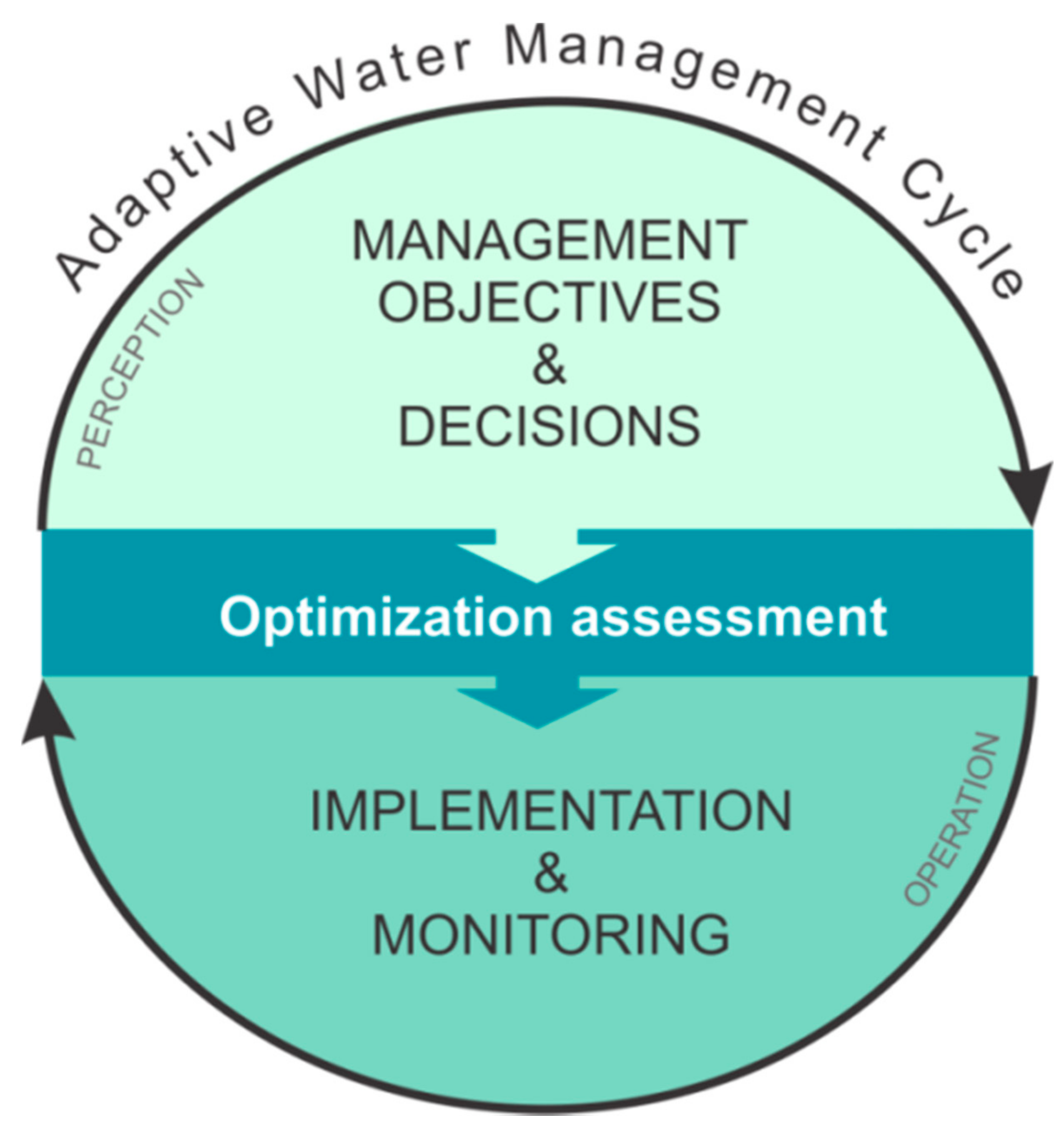
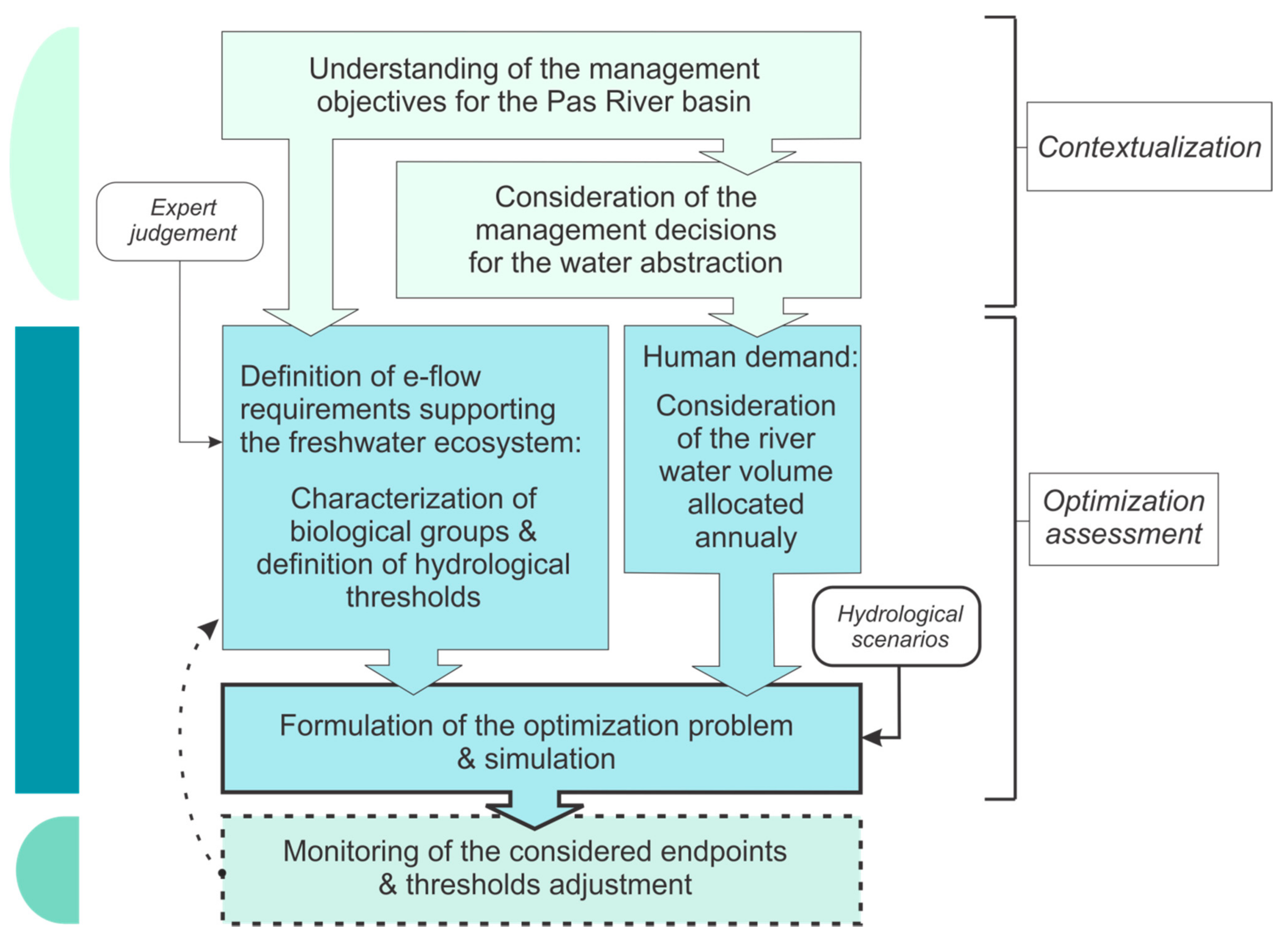
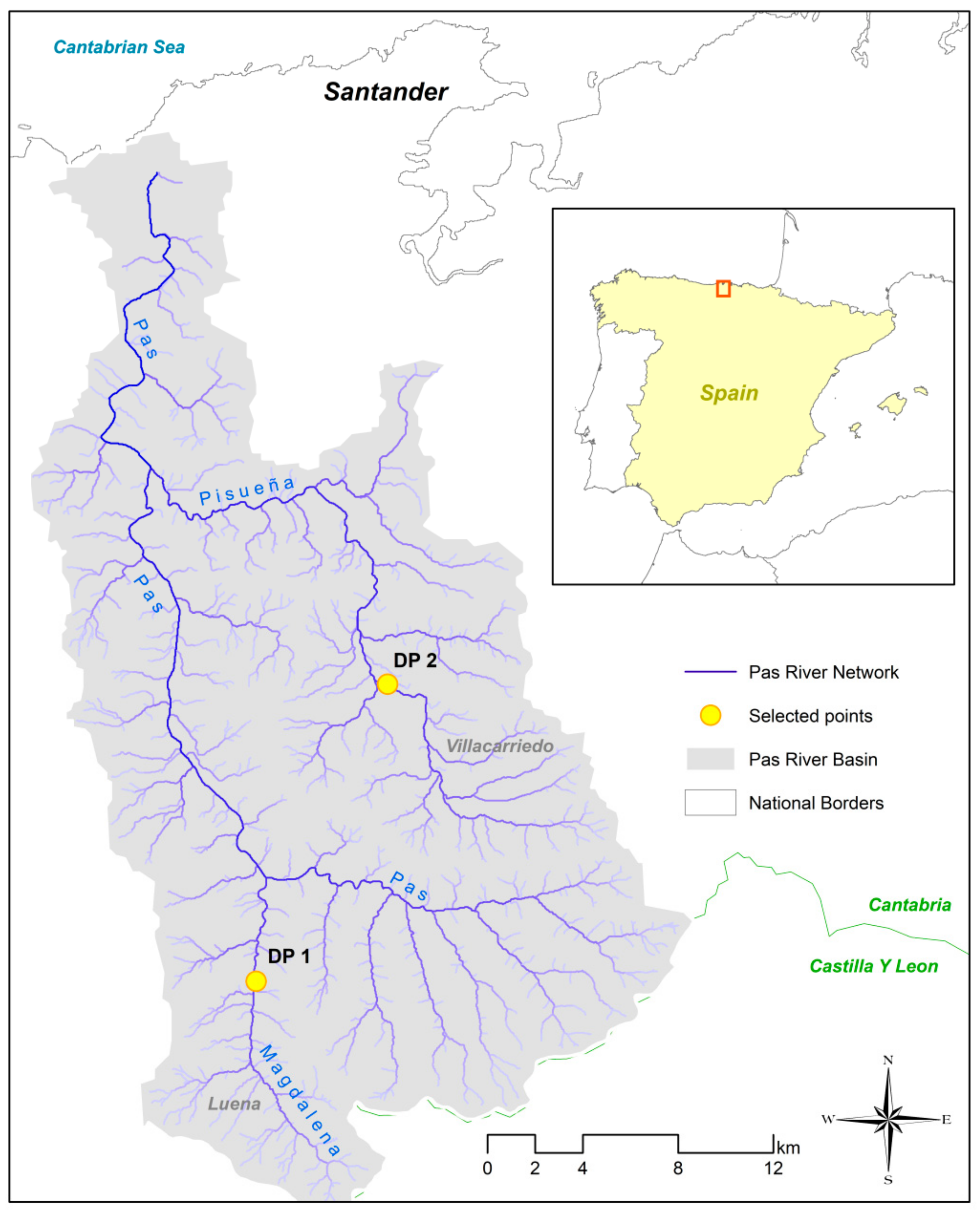
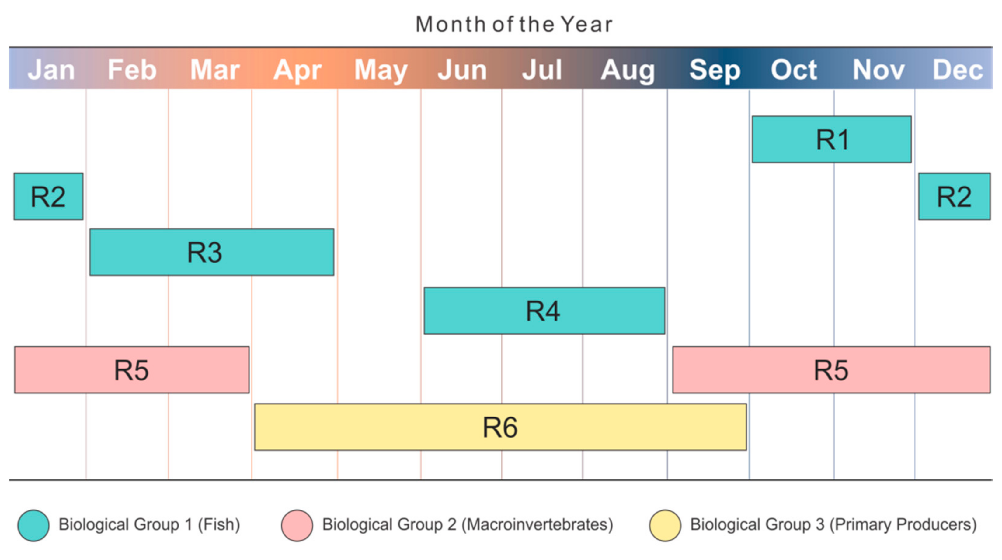
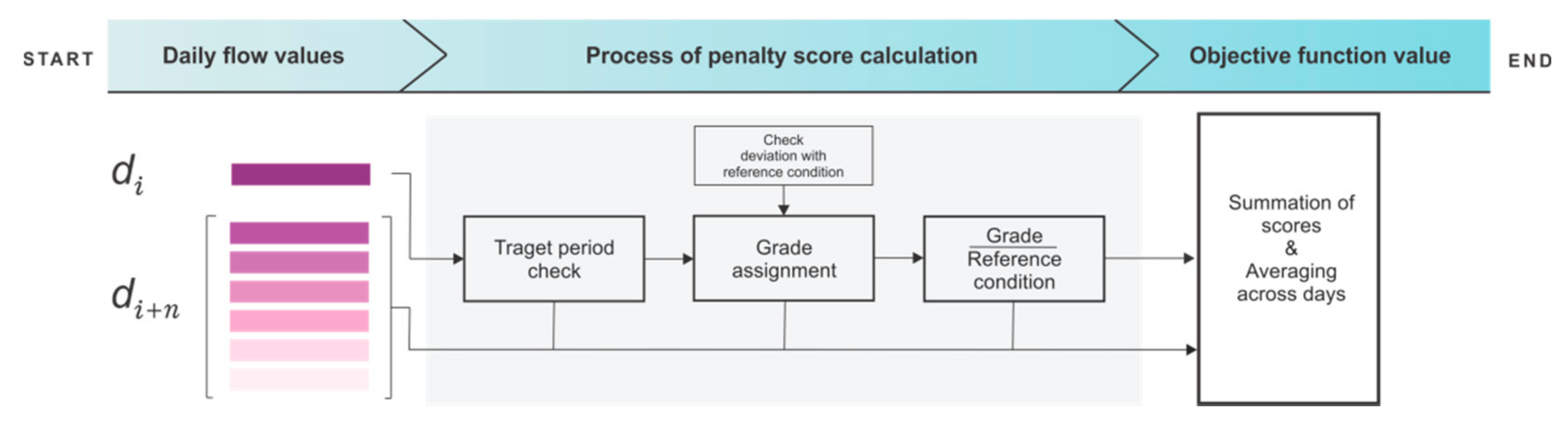
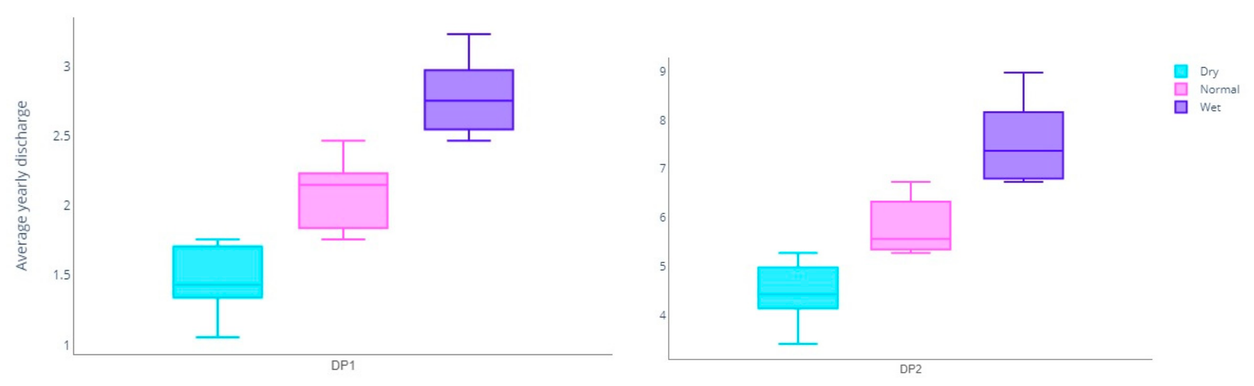
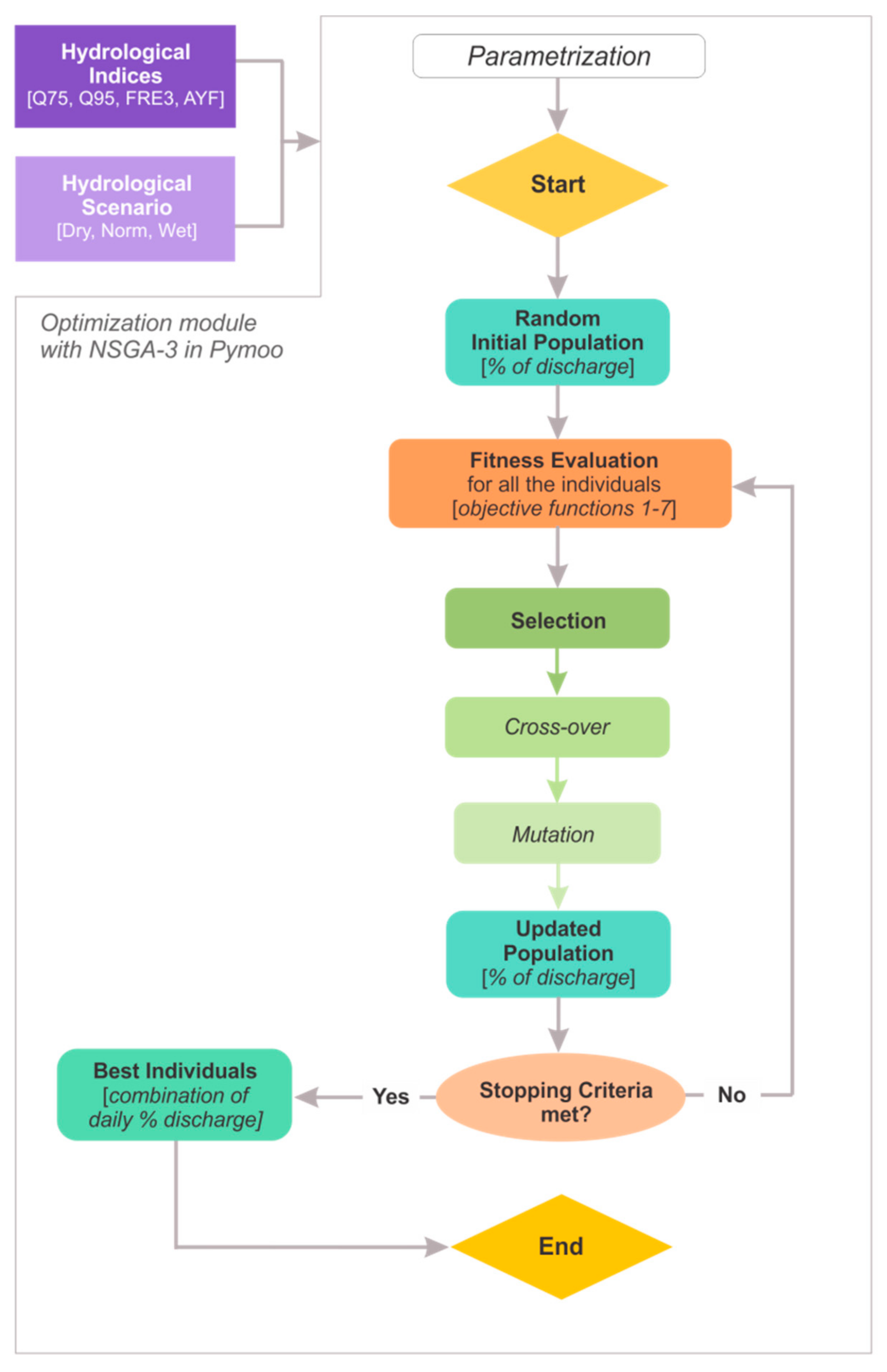
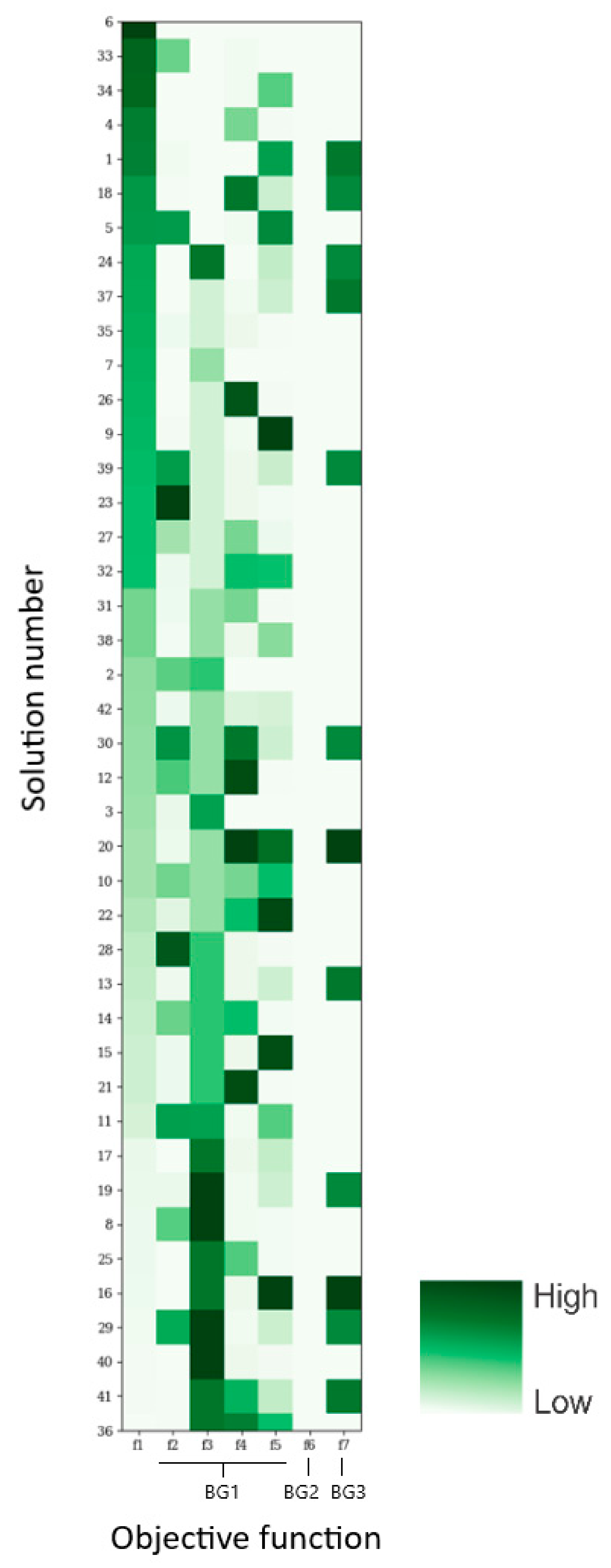
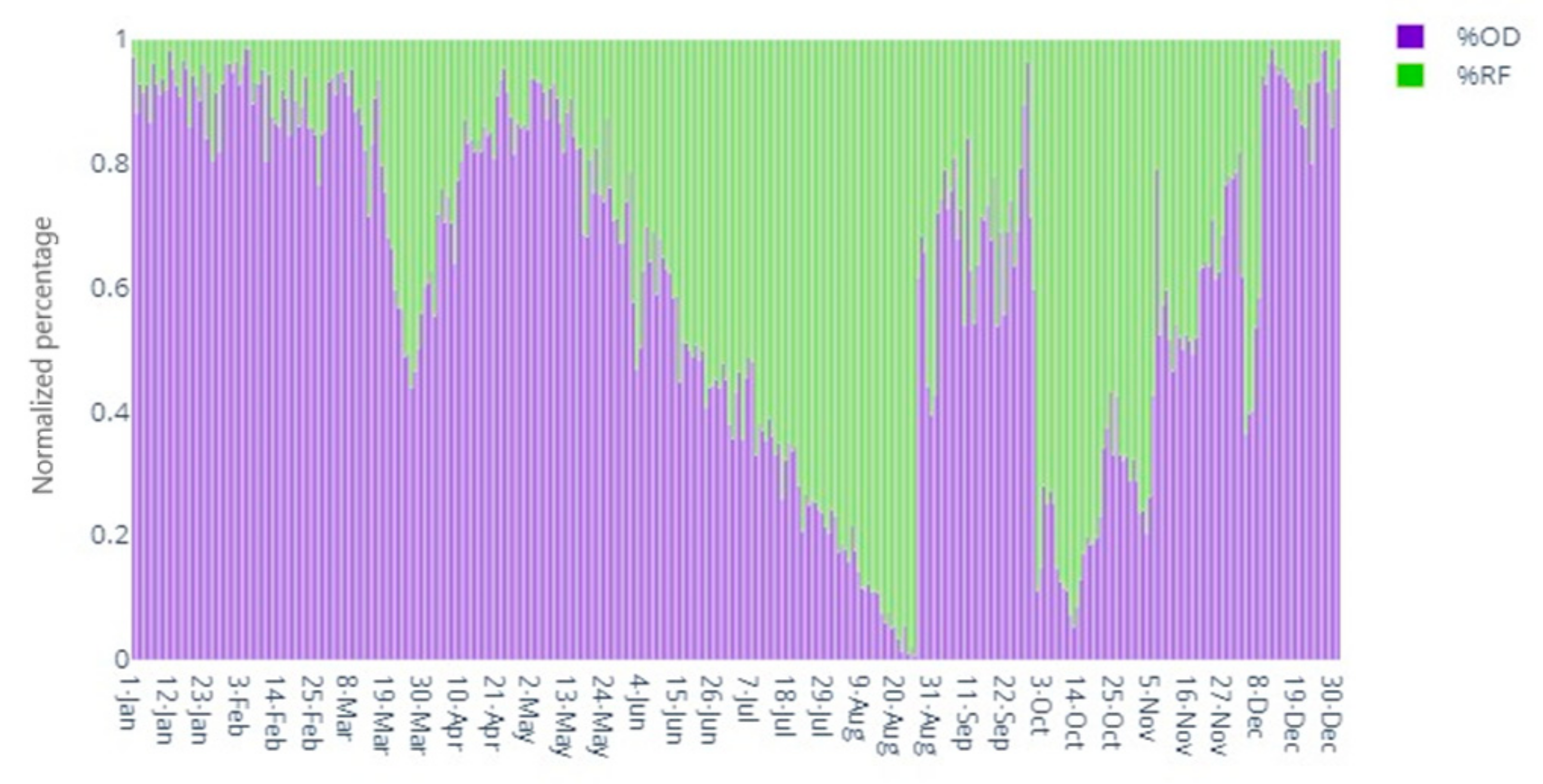
Table 1.
E-flow requirements considered in this study: The requirements define the hydrological conditions to be conserved in the river during the daily diversion operations throughout the year. Q95–Q75 is the flow value that is exceeded 95% and 75% of the time, respectively; FRE3 is the flow value that exceeds three times the median flow.
| Target Group | Requirement | Definition |
|---|---|---|
| Biological Group 1 | R1 | Q95 flow, full period |
| R2 | FRE3 flow, 21 days (consequent) | |
| R3 | Q95 flow, 45 days (consequent) | |
| R4 | Q95 flow, full period | |
| Biological Group 2 | R5 | Q75 flow, 5 events |
| Biological Group 3 | R6 | 10% average yearly flow, 70 days (consequent) |
Publisher’s Note: MDPI stays neutral with regard to jurisdictional claims in published maps and institutional affiliations. |
© 2021 by the authors. Licensee MDPI, Basel, Switzerland. This article is an open access article distributed under the terms and conditions of the Creative Commons Attribution (CC BY) license (https://creativecommons.org/licenses/by/4.0/).
Share and Cite
MDPI and ACS Style
Derepasko, D.; Peñas, F.J.; Barquín, J.; Volk, M. Applying Optimization to Support Adaptive Water Management of Rivers. Water 2021, 13, 1281. https://doi.org/10.3390/w13091281
AMA Style
Derepasko D, Peñas FJ, Barquín J, Volk M. Applying Optimization to Support Adaptive Water Management of Rivers. Water. 2021; 13(9):1281. https://doi.org/10.3390/w13091281
Chicago/Turabian StyleDerepasko, Diana, Francisco J. Peñas, José Barquín, and Martin Volk. 2021. "Applying Optimization to Support Adaptive Water Management of Rivers" Water 13, no. 9: 1281. https://doi.org/10.3390/w13091281
Note that from the first issue of 2016, this journal uses article numbers instead of page numbers. See further details here.