A Thermal Effect Model for the Impact of Vertical Groundwater Migration on Temperature Distribution of Layered Rock Mass and Its Application

Abstract

On the basis of the one-dimensional heat conduction–convection equation, a thermal effect model for vertical groundwater migration in the stratified rock mass was established, the equations for temperature distribution in layered strata were deduced, and the impacts of the vertical seepage velocity of groundwater and the thermal conductivity of surrounding rocks on the temperature field distribution in layered strata were analyzed. The proposed model was employed to identify the thermal convection and conduction regions at two temperature-measuring boreholes in coal mines, and the vertical migration velocity of groundwater was obtained through reverse calculation. The results show that the vertical temperature distribution of the layered rock mass is subject to the migration of the geothermal water; the temperature curve of the layered formation is convex when the geothermal water travels upward, but concave when the water moves downward. The temperature distribution in the stratified rock mass is also subject to the thermal conductivity of the rock mass; greater thermal conductivity of the rock mass leads to a larger temperature difference among regions of the rock mass, while weaker thermal conductivity results in a smaller temperature difference. A greater velocity of the vertical migration of geothermal water within the surrounding rock leads to a larger curvature of the temperature curve. The model was applied to a study case, which showed that the model could appropriately describe the variation pattern of the ground temperature in the stratified rock mass, and a comparison between the modeling result and the measured ground temperature distribution revealed a high goodness of fit of the model with the actual situation.

1. Introduction

Geothermal energy, a renewable energy, has shown great application prospects, and geothermal water is currently the most widely used form of geothermal energy around the world [1,2,3,4]. Coal, a reliable source of energy for many countries including China, accounts for 40% of all electric power generated worldwide. As the exploration and the development of coal intensify, more medium- and low-temperature geothermal water resources have been found in coal measure strata, which provides a basis for further investigation and evaluation of geothermal water resources. In coalfield exploration, temperature measurement is generally carried out along with geological drilling. Migration of geothermal water will affect the temperature of the surrounding rock mass; thus, in areas that witness seepage of geothermal water, the local temperature will differ substantially from that in other areas of the rock mass due to the heat transfer from the water. In this case, the temperature curve can be used to identify where the geothermal water occurs, as well as the temperature and seepage conditions of the water; thus, it can be used to lay a theoretical foundation for further analysis of geothermal water resources.

Much research effort has been devoted to the heat transfer of temperature distribution in layered formations and to the heat exchange between the surrounding rock and the geothermal water. Jaeger and Carslaw (1959) explained the heat exchange process between the upward-moving geothermal water and the surrounding rock using the cooling equation of hot water well, which provided a theoretical basis for later studies on the distribution of the temperature fields in surrounding rocks under vertical seepage of groundwater [5]. By solving the one-dimensional heat conduction–convection equation, Bredehoeft et al. (1965) identified the relationship among the vertical depth, permeability, and surrounding rock temperature distribution, which laid a foundation for the identification of vertical movement of groundwater using temperature measurement profiles [6]. Sorey (1971) proved that the one-dimensional heat conduction–convection equation could be employed to identify the characteristics of the temperature curve of the rock formation under groundwater migration with a vertical seepage velocity of 10⁻⁸ m/s [7]. Bodvarsson (1982) investigated abnormal temperature distribution within faults caused by vertical movements of groundwater and estimated the potential recharge rate of the faults to the hydrothermal system using the one-dimensional heat conduction–convection equation [8]. By applying the finite element method to an analysis of the temperature field distribution of hot water wells and heat transfer to surrounding rocks, Zhang and Xiong (1984), from the Institute of Geology, Chinese Academy of Sciences, revealed the functional relationship between wellhead temperature and heat storage temperature, which provided a new method to study the temperature distribution of underground surrounding rocks [9]. Lu et al. (1996) extended the one-dimensional heat conduction–convection equation proposed by Bredehoeft and proved that, when parameters such as thermal conductivity, density, and specific heat capacity were known, the migration velocity of the groundwater could be calculated according to the measured temperature in the borehole [10]. Xu et al. (2000) established a thermal effect model of vertical fluid migration based on the properties of heat transfer by vertical fluid percolation, and they discussed the feasibility of using the temperature curve for reverse calculation of the reservoir temperature and estimation of the fluid flow in faults [11]. Liu et al. (2007) calculated the permeability coefficient of the fractured rock mass by combining the temperature field and the statistical method, and they further expanded the scope of seepage parameters that could be identified by the temperature measurement curve [12]. Gong et al. (2010) analyzed the seepage direction of groundwater, as well as the storage conditions of oil and gas, by using the curve of temperature distribution in drilling, and they expanded the application of the temperature curve to identification of seepage in geoformations [13]. Up to now, the technology of identifying geothermal resources on the basis of the temperature curve measured in boreholes has gradually matured, and it has been widely used in the analysis of the genetic mechanism and distribution characteristics of geothermal resources [14,15,16,17].

To the best of the authors’ knowledge, many scholars have studied the thermal effect of one-dimensional vertical groundwater migration on the temperature distribution of rock masses, and they have successfully applied it to the identification of conduction and convection segments in the temperature curve obtained in temperature-measuring boreholes, which has made an outstanding contribution to the development and application of theoretical geothermal research. However, systematic summaries of vertical migration and thermal effect characteristics of geothermal water in the stratified rock mass have not been reported. Previous research results showed that the coal measure strata are typical stratified formations, and parameters such as rock thermal conductivity, porosity, groundwater seepage velocity, and specific heat capacity in stratified formations have a direct impact on the distribution of temperature fields in these formations. Therefore, in the present work, on the basis of the one-dimensional heat conduction–convection equation, a thermal effect model of vertical fluid migration in the stratified rock mass was established; the impact of the vertical seepage velocity and surrounding rock thermal conductivity on temperature field distribution in the formation was analyzed. The proposed model was applied to two coal mines, Guqiao and Dingji Mines, to identify the temperature curves at two temperature-measuring boreholes, as well as to reverse-calculate the vertical migration velocity of groundwater. The research result is expected to provide a theoretical basis for future development of geothermal water resources.

2. Model Establishment

2.1. One-Dimensional Geothermal Field of Homogeneous Rock Mass

In the present work, it is assumed that the underground rock mass is composed of an ideal water-resisting layer free from water penetration. The rock strata are all isotropic and homogeneous conductors of heat, the total thickness of the rock mass is h, and the ground temperature distribution of surrounding rocks is a thermal conduction temperature field. When the heat transfer is stable, the vertical temperature distribution can be expressed by a one-dimensional mathematical model, as shown below.

$$k\frac{{\partial }^{2}T}{\partial z^2}=0.$$

(1)

Then, the ground temperature at a depth of z is $T=T_0+\frac{T_1-T_0}{h}z$, where T₀ and T₁ represent the known temperatures of the upper and lower boundary of the rock stratum, respectively.

In areas where movements of groundwater are observed, the temperature field is affected by both conduction and convection of heat. When the groundwater moves fast in a geological structure, there is a temperature gap between the water-moving area and the surrounding rock mass, leading to heat exchange in between. In general, a one-dimensional mathematical model can be established to describe the distribution of the ground temperature T at any depth z [5,18]. The model is shown below.

$${\rho }_1{c}_1\frac{\partial T}{\partial t}=(1-n)k\frac{{\partial }^{2}T}{\partial z^2}+n{\rho }_w{c}_w{v}_z\frac{\partial T}{\partial z}-2a\left(T-T_C\right),$$

(2)

where a is heat exchange coefficient between the groundwater and the surrounding rock mass, k is thermal conductivity of the rock (W·(m·°C)⁻¹), c_w and ρ_w are the specific heat capacity (J/(kg·°C)) and density (kg/m³) of the groundwater, respectively, c₁ and ρ₁ are the specific heat capacity (J/(kg·°C)) and density (kg/m³) of the groundwater–rock mixture, respectively, n is porosity of the surrounding rock mass, T_c is the temperature of surrounding rock mass (°C), and t is time (s).

In the actual strata, the ground water moves vertically at a small rate. During the movement, the water is in full contact with the surrounding rock, and the water flow at higher temperatures from deep down slowly warms up the surrounding rock. In this case, the temperature difference between the water flow and the surrounding rock will gradually decrease, and the heat exchange between the two can be ignored at the end. Therefore, we assume a = 0, and Equation (2) can be simplified as follows:

$${\rho }_1{c}_1\frac{\partial T}{\partial t}=(1-n)k\frac{{\partial }^{2}T}{\partial z^2}+n{\rho }_w{c}_w{v}_z\frac{\partial T}{\partial z}.$$

(3)

When the flow migration time $t\to \infty$, a thermal balance occurs between the water flow and the surrounding rock, which is considered as a thermal steady state. Thus, Equation (3) can be transformed into

$$(1-n)k\frac{{\partial }^{2}T}{\partial z^2}+n{\rho }_w{c}_w{v}_z\frac{\partial T}{\partial z}=0.$$

(4)

Here, the surrounding rock mass is assumed to be an isotropic and homogeneous heat conductor. T₀ and T₁ are known temperatures of the upper and lower boundaries of the rock, respectively. Then, the analytical solution of Equation (4) can be expressed as

$$T=T_0+(T_1-T_0)\frac{e^{{\beta }_{1}z}-1}{e^{{\beta }_{1}h}-1},$$

(5)

where ${\beta }_1=\frac{n{c}_w{\rho }_w{v}_z}{\left(1-n\right)k}$.

2.2. One-Dimensional Geothermal Field of Stratified Rock Mass

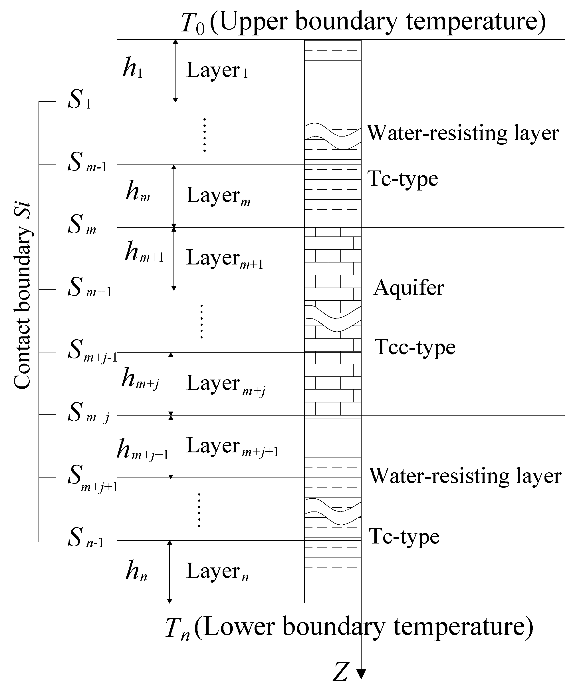
According to the one-dimensional mathematical model for the temperature distribution of thermal conduction and conduction–convection of the homogeneous rock mass mentioned above, the thermal effect model of vertical fluid migration of the stratified rock mass is established. There are two types of temperature fields in the model, namely, the thermal conduction (Tc-type) and thermal conduction–convection (Tcc-type) temperature fields. The model consists of n layers, in which the upper layer m is a Tc-type temperature field, the middle layer j is a Tcc-type temperature field, and the lower layer n − m + j is a Tc-type temperature field (Figure 1). It is assumed that the contact boundaries of adjacent rock strata are S₁, S₂, ……, S_n−1, with temperatures of T₁, T₂, ……, T_m (interfacial temperatures within the m layer), T_m+1, T_m+2, ……, T_m+j (interfacial temperatures in the j layer), and T_m+j+1, T_m+j+2, ……, T_n−1 (interfacial temperatures within the n − m + j layer). The temperature of the interface between two adjacent temperature fields (z = h₁ + h₂ + …… + h_n−1) is the same, set to T_n−1. The temperature T₀ at z = 0 and the temperature T_n at z = h₁ + h₂ + …… + h_n are known. The vertical temperature distribution in the layer i (1 ≤ i ≤ n) is derived below.

The “iterative” and the “chasing” derivation methods are often used for the establishment of models. The “chasing method” is to establish an iterative equation between the temperature T_i−1 and T_i of the two adjacent strata and the known temperature T₀ of the upper surface; the iteration continues until i = n. According to the obtained iterative equation, the known lower surface temperature T_n was used for substitution in the equation to complete the “chasing” process, after which the relation equation for the temperature of one layer in the model (T_i) expressed by the known T₀ and T_n was obtained. The results are described below.

(1)

The temperature of each layer in the Tc-type temperature field of the upper m layer is expressed as

$$T=T_{i-1}+\frac{T_i-T_{i-1}}{h_i}\left(Z-{\displaystyle \sum _{k=0}^{i-1}{h}_k}\right)(1\le i\le m, {\displaystyle \sum _{k=0}^{i-1}{h}_k}<Z\le {\displaystyle \sum _{k=0}^i{h}_k}).$$

(6)

The temperature gradient is

$$\frac{\partial T}{\partial Z}=\frac{T_i-T_{i-1}}{h_i}(1\le i\le m).$$

(7)

The boundary between the i − 1 layer and the i layer is the contact surface of two solids. According to the law of heat conduction, the heat flux density of the fluid flowing through the contact surface of two objects is equal, i.e.,

$$-k_{i-1}·{\frac{\partial T}{\partial Z}|}_{Si-1}=-k_i·{\frac{\partial T}{\partial Z}|}_{Si-1}.$$

(8)

It can be concluded that the temperature of the contact surface of any two adjacent layers is

$$T_{i-1}=\frac{T_i+{\zeta }_{i-1}{T}_0}{1+{\zeta }_{i-1}}{T}_{i-1}=\frac{T_i+{\zeta }_{i-1}{T}_0}{1+{\zeta }_{i-1}}(1<i\le m),$$

(9)

where ${\zeta }_{i-1}=\frac{k_1{k}_2{k}_{3\dots \dots }{k}_{i-1}{h}_i}{h_1{k}_2{k}_3\dots \dots k_i+k_1{h}_2{k}_3\dots \dots k_i+\dots \dots +k_1{k}_2{k}_3\dots \dots h_{i-1}{k}_i}$.

(2)

The temperature of each layer in the Tcc-type temperature field in the middle layer j is expressed as follows:

$$T=T_{i-1}-(T_{i-1}-T_i)\frac{e^{{\beta }_i(z-{\displaystyle \sum _{k=0}^{i\sum 1}{h}_k})}-1}{(e^{{\beta }_i·h_i}-1)}.$$

(10)

The geothermal gradient is

$$\frac{\partial T}{\partial Z}=-(T_{i-1}-T_i)\frac{{\beta }_i{e}^{{\beta }_i(z-{\displaystyle \sum _{k=0}^{i\sum 1}{h}_k})}}{(e^{{\beta }_i·h_i}-1)} (m+1\le i\le m+j,{\displaystyle \sum }_{k=0}^{i-1}{h}_k\le Z<{\displaystyle \sum }_{k=0}^i{h}_k).$$

(11)

As the temperature T_m of the interface between the m layer and m + 1 layer is the temperature of the interface between the Tc-type and Tcc-type temperature fields, the temperatures of these two layers need to be calculated separately. On the contact surface between the m layer and the m + 1 layer, the following equation holds:

$$-k_m·{\frac{\partial T}{\partial Z}|}_{Sm}=-k_{m+1}·{\frac{\partial T}{\partial Z}|}_{Sm}.$$

(12)

As per Equation (12), the following equation is obtained:

$$-k_m·\frac{T_m-T_{m-1}}{h_m}=k_{m+1}(T_m-T_{m+1})\frac{{\beta }_{m+1}}{e^{{\beta }_{m+1}·h_{m+1}}-1}.$$

(13)

Thus, the temperature of the contact surface is

$$T_m=\frac{T_{m+1}+T_0{\psi }_m}{1+{\psi }_m},$$

(14)

where ${\psi }_m=\frac{{\zeta }_{m-1}{\gamma }_m}{1+{\zeta }_{m-1}}$, and ${\gamma }_m=\frac{k_m·(e^{{\beta }_{m+1}·h_{m+1}}-1)}{k_{m+1}·{\beta }_{m+1}·h_m}$.

The m + 1 to m + j layers feature a Tcc-type temperature field, and, on the contact surface of two adjacent layers, the following equation holds:

$$-k_i·{\frac{\partial T}{\partial Z}|}_{Si}=-k_{i+1}·{\frac{\partial T}{\partial Z}|}_{Si}.$$

(15)

As per Equation (15), the following equation is obtained:

$$k_i(T_{i-1}-T_i)\frac{{\beta }_i{e}^{{\beta }_i·h_i}}{e^{{\beta }_i·h_i}-1}=k_{i+1}(T_i-T_{i+1})\frac{{\beta }_{i+1}}{e^{{\beta }_{i+1}·h_{i+1}}-1}.$$

(16)

Thus, the temperature of the contact surface can be obtained as follows:

$$T_i=\frac{T_{i+1}+T_0{\psi }_i}{1+{\psi }_i} (m+1\le i\le m+j-1),$$

(17)

where ${\psi }_i=\frac{{\psi }_{i-1}{\theta }_i}{1+{\psi }_{i-1}}$, and ${\theta }_i=\frac{k_i·{\beta }_i(e^{{\beta }_{i+1}·h_{i+1}}-1)}{k_{i+1}{\beta }_{i+1}·(e^{{\beta }_i·h_i}-1)}{e}^{{\beta }_i·h_i}$ ($m+1\le i\le m+j-1$).

(3)

The temperature of each stratum in the Tc-type temperature field in the lower n-m-j layer is expressed as follows:

$$T=T_{i-1}+\frac{T_i-T_{i-1}}{h_i}\left(Z-{\displaystyle \sum _{k=0}^{i-1}{h}_k}\right) (m+j\le i\le n, {\displaystyle \sum _{k=0}^{i-1}{h}_k}<Z\le {\displaystyle \sum _{k=0}^i{h}_k}).$$

(18)

The geothermal gradient is

$$\frac{\partial T}{\partial Z}=\frac{T_i-T_{i-1}}{h_i}\hspace{1em}\hspace{1em}\hspace{1em}\hspace{1em}\hspace{1em}(m+j\le i\le n).$$

(19)

As the temperature T_m+j of the interface between the m + j layer and the m + j + 1 layer is the temperature of the interface between the Tc-type and Tcc-type temperature fields, the temperature for the two layers should be calculated separately. On the contact surface between the m + j layer and the m + j + 1 layer, there is

$$-k_{m+j}·{\frac{\partial T}{\partial Z}|}_{Sm+j}=-k_{m+j+1}·{\frac{\partial T}{\partial Z}|}_{Sm+j}.$$

(20)

As per Equation (20), the following equation is obtained:

$$k_{m+j}(T_{m+j-1}-T_{m+j})\frac{{\beta }_{m+j}·e^{{\beta }_{m+j}·h_{m+j}}}{(e^{{\beta }_{m+j}·h_{m+j}}-1)}=-k_{m+j+1}\frac{T_{m+j+1}-T_{m+j}}{h_{m+j+1}}.$$

(21)

The temperature of the contact surface can be obtained as follows:

$$T_{m+j}=\frac{T_{m+j+1}+T_0{\epsilon }_{m+j}}{1+{\epsilon }_{m+j}},$$

(22)

where ${\epsilon }_{m+j}=\frac{{\lambda }_{m+j}{\psi }_{m+j-1}}{1+{\psi }_{m+j-1}}$, and ${\lambda }_{m+j}=\frac{k_{m+j}·{\beta }_{m+j}·e^{{\beta }_{m+j}·h_{m+j}}{h}_{m+j+1}}{k_{m+j+1}·(e^{{\beta }_{m+j}·h_{m+j}}-1)}$.

Similarly,

$$T_i=\frac{T_{i+1}+T_0{\epsilon }_i}{1+{\epsilon }_i} (m+j+1\le i\le n-1),$$

(23)

where ${\epsilon }_i=\frac{{\alpha }_i·{\epsilon }_{i-1}}{1+{\epsilon }_{i-1}}$, and ${\alpha }_i=\frac{k_i{h}_{i+1}}{k_{i+1}{h}_i}$ ($m+j+1\le i\le n-1$).

The calculation specified in Equations (1)–(3) is a “chasing” process using the upper surface temperature T₀ already given in the model. On that basis, all other unknown variables can be obtained using the chasing method based on the known lower surface temperature T_n. The relationship among the temperatures T_i, T₀, and T_n of each layer can be described as follows:

$$T_i=\{\begin{array}{c}{T}_0+\frac{T_n-T_0}{{\displaystyle \prod _{k=i}^{m-1}\left(1+{\zeta }_k\right)}{\displaystyle \prod _{k=m}^{m+j-1}\left(1+{\psi }_k\right)}{\displaystyle \prod _{k=m+j}^{n-1}\left(1+{\epsilon }_k\right)}} \left(1\le i\le m-1\right)\hfill \\ T_0+\frac{T_n-T_0}{{\displaystyle \prod _{k=i}^{m+j-1}\left(1+{\psi }_k\right)}{\displaystyle \prod _{k=m+j}^{n-1}\left(1+{\epsilon }_k\right)}}\left(m\le i\le m+j-1\right)\hfill \\ T_0+\frac{T_n-T_0}{{\displaystyle \prod _{k=i}^{n-1}\left(1+{\epsilon }_k\right)}} \left(m+j\le i\le n-1\right)\hfill \end{array},$$

(24)

where, T_i = T₀, T_n, when i = 0, n.

Upon substituting Equation (24) into the temperature distribution equations in the chasing process specified in Equations (1)–(3), the equation of the temperature distribution in the stratified rock mass can be obtained.

$$T=\{\begin{array}{l}{T}_0+\frac{T_n-T_0}{{\displaystyle \prod _{k=i-1}^{m-1}\left(1+{\zeta }_k\right)}{\displaystyle \prod _{k=m}^{m+j-1}\left(1+{\psi }_k\right)}{\displaystyle \prod _{k=m+j}^{n-1}\left(1+{\epsilon }_k\right)}}+\frac{(T_n-T_0){\zeta }_{i-1}}{{\displaystyle \prod _{k=i-1}^{m-1}\left(1+{\zeta }_k\right)}{\displaystyle \prod _{k=m}^{m+j-1}\left(1+{\psi }_k\right)}{\displaystyle \prod _{k=m+j}^{n-1}\left(1+{\epsilon }_k\right)}}·\frac{z-{\displaystyle \sum _{k=0}^{i-1}{h}_k}}{h_i} \left(0<i\le m\right)\\ T_0+\frac{T_n-T_0}{{\displaystyle \prod _{k=i-1}^{m+j-1}\left(1+{\psi }_k\right)}{\displaystyle \prod _{k=m+j}^{n-1}\left(1+{\epsilon }_k\right)}}+\frac{\left(T_n-T_0\right){\psi }_{i-1}}{{\displaystyle \prod _{k=i-1}^{m+j-1}\left(1+{\psi }_k\right)}{\displaystyle \prod _{k=m+j}^{n-1}\left(1+{\epsilon }_k\right)}}·\frac{e^{{\beta }_i(z-{\displaystyle \sum _{k=0}^{i-1}{h}_k})}-1}{e^{{\beta }_i·h_i}-1} \left(m<i\le m+j\right)\\ T_0+\frac{T_n-T_0}{{\displaystyle \prod _{k=i-1}^{n-1}\left(1+{\epsilon }_k\right)}}+\frac{\left(T_n-T_0\right){\epsilon }_{i-1}}{{\displaystyle \prod _{k=i-1}^{n-1}\left(1+{\epsilon }_k\right)}}·\frac{z-{\displaystyle \sum _{k=0}^{i-1}{h}_k}}{h_i}\left(m+j<i\le n\right)\end{array}.$$

(25)

This can be applied to the following formula:

$$\left({\displaystyle \sum _{k=0}^{i-1}{h}_k}<Z\le {\displaystyle \sum _{k=0}^i{h}_k}, 1\le i\le n\right),$$

(26)

where h_i is the thickness of layer i (m), k_i is the thermal conductivity of the stratum in layer i (W·(m·°C)⁻¹), T₀ is the known temperature at the upper boundary of the first layer (°C), T_n is the known temperature at the lower boundary of layer n (°C), ${\beta }_i=\frac{n_i{c}_w{\rho }_w{v}_z{}_i}{\left(1-n_i\right)k_i}$ (n_i is the porosity of each layer in the convection zone), $v_{zi}$ is the volume velocity of groundwater in the i layer along the z axis (m³/s), and v_z is positive when the water moves downward, while it is negative if the water moves upward.

3. Parameter Analysis

3.1. Effect of Seepage Velocity on Geothermal Field

In the present work, it is assumed that a geological formation consists of three layers: the upper thermal conduction layer comprising three rock strata, the middle thermal conduction–convection layer comprising three rock strata, and the lower thermal conduction layer also comprising three rock strata. The upper surface temperature of the model (T₀) is 35 °C, and the lower surface temperature (T₉) is 43.1 °C. The model upper surface elevation (H₀) is −500 m, and the lower surface elevation (H₉) is −770 m. The specific heat capacity (C_w) and density (ρ) of water are 4200 J/(kg·°C) and 1000 kg/m³, respectively. It is assumed that the thermal conductivity of the surrounding rock remains constant, and the rock porosity (n) in the thermal convection area is 0.15. The groundwater seepage velocity (v) was set to ±[0.5, 1, 1.5, 2] × 10⁻⁸ m³/s. The relationship between the vertical temperature and the buried depth z in the model was analyzed. Specific parameters of the model are shown in

Table 1. Model parameters.

Temperature Field	Layer	Thickness (m)	Thermal Conductivity k (W·(m·°C)−1)	Aquifer Location
Tc-type	1	30	2.0	Water-resisting layer
	2	30	2.0
	3	30	2.0
Tcc-type	4	30	2.0	Aquifer
	5	30	2.0
	6	30	2.0
Tc-type	7	30	2.0	Water-resisting layer
	8	30	2.0
	9	30	2.0

.

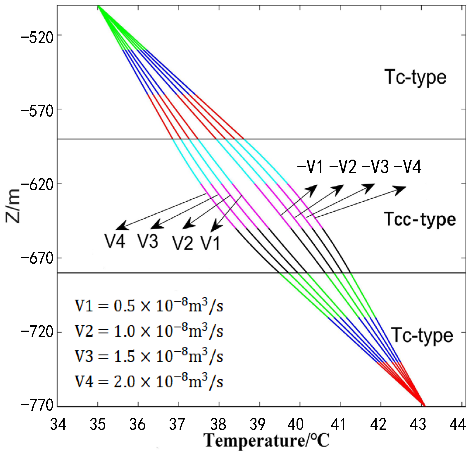
According to the above established model, the software Matlab (MathWorks Inc., Natick, MA, USA) was used to program Equation (25) to obtain the temperature–buried depth (z) curve along the vertical direction under different seepage velocities, as shown in Figure 2.

As Figure 2 shows, the geothermal curve presents a linear distribution in the Tc-type region. Under the action of groundwater seepage, the curve in the Tcc-type region is convex when the seepage is upward, and it is concave when the seepage is downward. In general, the ground temperature in the model is higher when the groundwater percolates upward than when it percolates downward. In addition, a lower seepage velocity leads to a smaller curvature of the curve in the Tcc-type region. When the seepage velocity is close to 0, the curve in the Tcc-type region presents a linear distribution, which is similar to that in the Tc-type region. This indicates that the presence and migration of groundwater are among the major factors that affect the distribution of the temperature field.

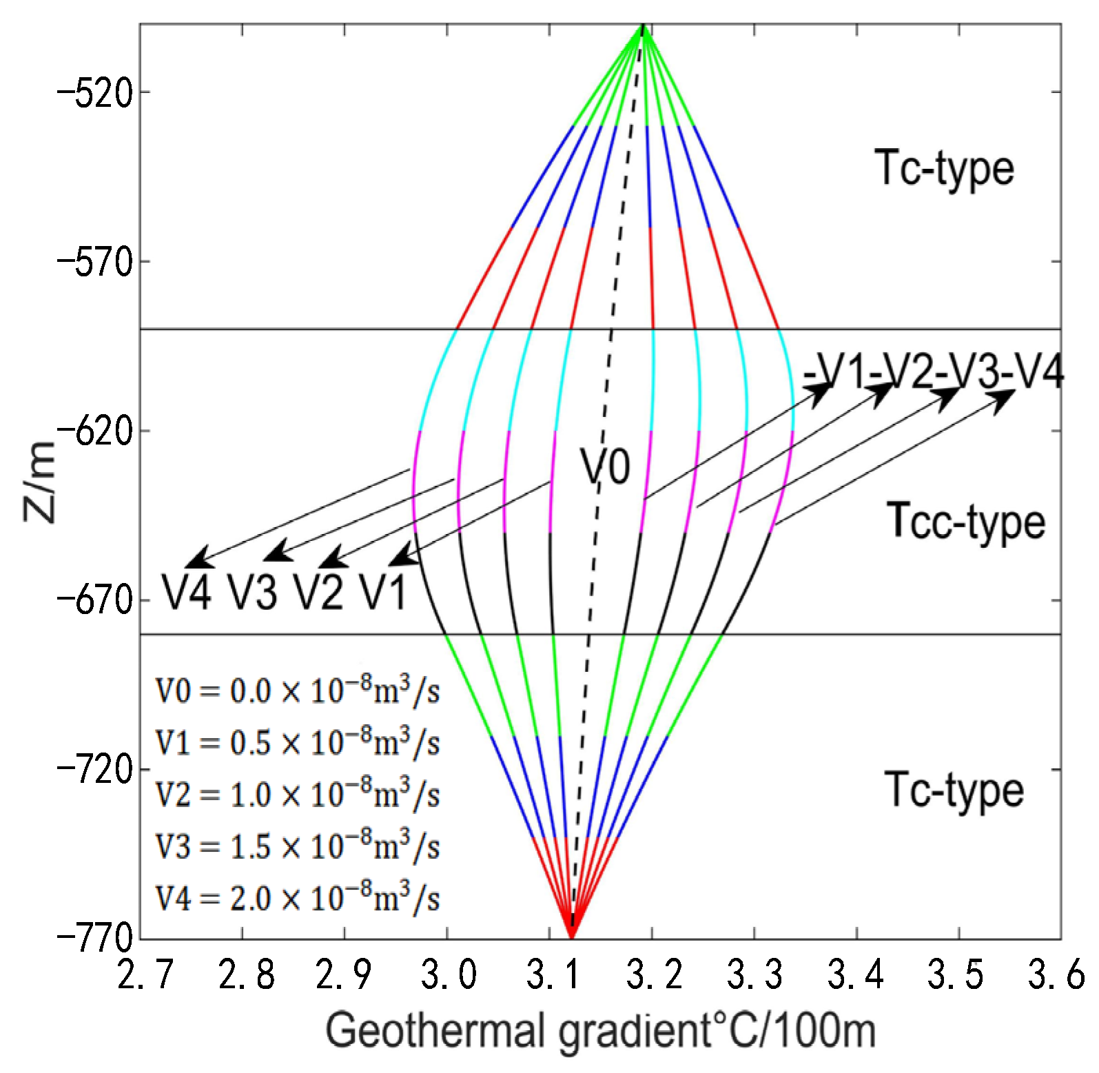
According to the calculation equations for the geothermal gradient, the variation pattern of the geothermal gradient with the buried depth z under different seepage velocities can be obtained. Curves in Figure 3 show the specific variation patterns.

As Figure 3 shows, when there is groundwater seepage in the surrounding rock, the geothermal gradient changes accordingly. When the seepage is upward, the gradient increases obviously, and a greater seepage velocity leads to a larger increase in the gradient. On the contrary, the gradient decreases when the groundwater percolates downward, and a greater seepage velocity leads to a more drastic decrease in the gradient. When the seepage velocity is 0, the curve is a straight line, and, in this case, the Tcc-type temperature field is the only temperature field in the surrounding rock. This indicates that the formation of the Tcc-type temperature field entails not only the presence but also migration of groundwater.

3.2. Effect of Thermal Conductivity of Rock on Temperature Field

The rock thermal conductivity, a thermophysical parameter of rocks, mainly reflects the heat transfer characteristics of rocks and is also a necessary parameter for the calculation of the terrestrial heat flow value (Wu et al., 2019). In order to facilitate the analysis of the influence of rock thermal conductivity on the geothermal gradient distribution, the thermal conductivity was set to increase by values of equal differences. The thermal conductivity of each layer in the rock mass along the vertical direction is shown in

Table 2. Design schemes of thermal conductivity of surrounding rocks.

	Layer	1	2	3	4	5	6	7	8	9	Variance
Scheme		Thermal Conductivity k (W·(m·°C)−1)
1		4.1	3.7	3.3	2.9	2.5	2.1	1.7	1.3	0.9	1.07
2		3.3	3.1	2.9	2.7	2.5	2.3	2.1	1.9	1.7	0.27
3		2.5	2.5	2.5	2.5	2.5	2.5	2.5	2.5	2.5	0.00
4		1.7	1.9	2.1	2.3	2.5	2.7	2.9	3.1	3.3	0.27
5		0.9	1.3	1.7	2.1	2.5	2.9	3.3	3.7	4.1	1.07

.

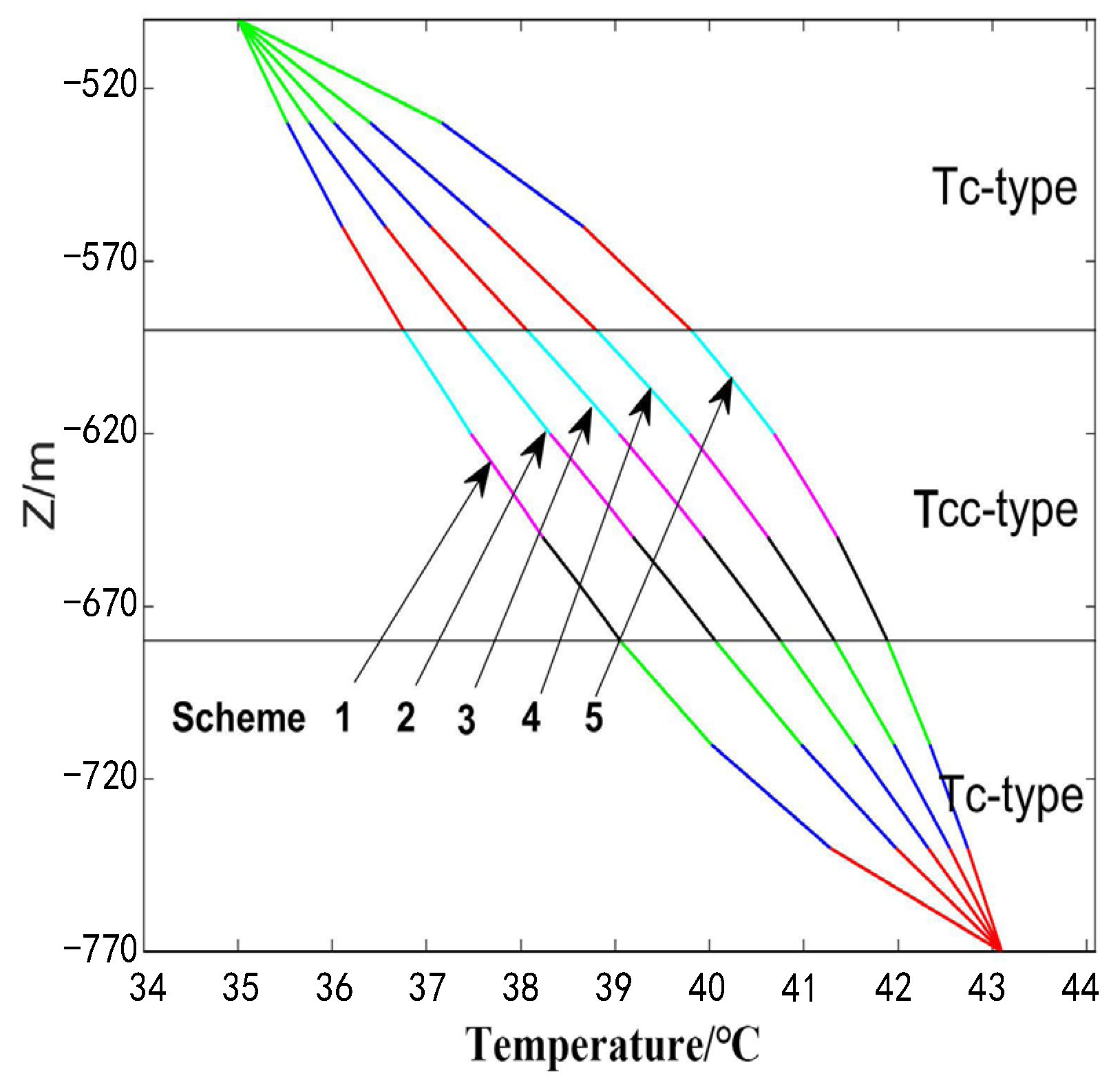
As Table 2 shows, the rock thermal conductivity of the five schemes was set to decrease or increase by an equal difference of 0, ±0.2, or ±0.4 along the vertical direction, and the mean conductivity of all the schemes remained at 2.5 k/W·(m·°C)⁻¹; the seepage velocity was set to v = −1 × 10⁻⁸ m³/s. The change pattern of the ground temperature with the buried depth z under the five schemes of rock thermal conductivity was obtained, as shown by the curves in Figure 4.

As shown in Table 2, the low-thermal-conductivity area in Scheme 1 was located at the lower part of the model, while that in Scheme 5 was located at the upper part of the model. As shown in Figure 4, in Scheme 1 and Scheme 5, the high-geothermal-gradient area corresponded to the low-thermal-conductivity area. This is because the rock mass with low thermal conductivity blocked the transfer of heat that moved up from deep, and the temperature at the upper and lower boundaries of the rock mass varied greatly, resulting in a large geothermal gradient inside the thermal conductivity formation. In addition, comparison of the thermal conductivity variances of all five schemes revealed that a greater variance of thermal conductivity, i.e., a greater difference in the thermal conductivity of the rock mass in the vertical direction, resulted in a greater curvature of the temperature–z curve.

4. Case Study

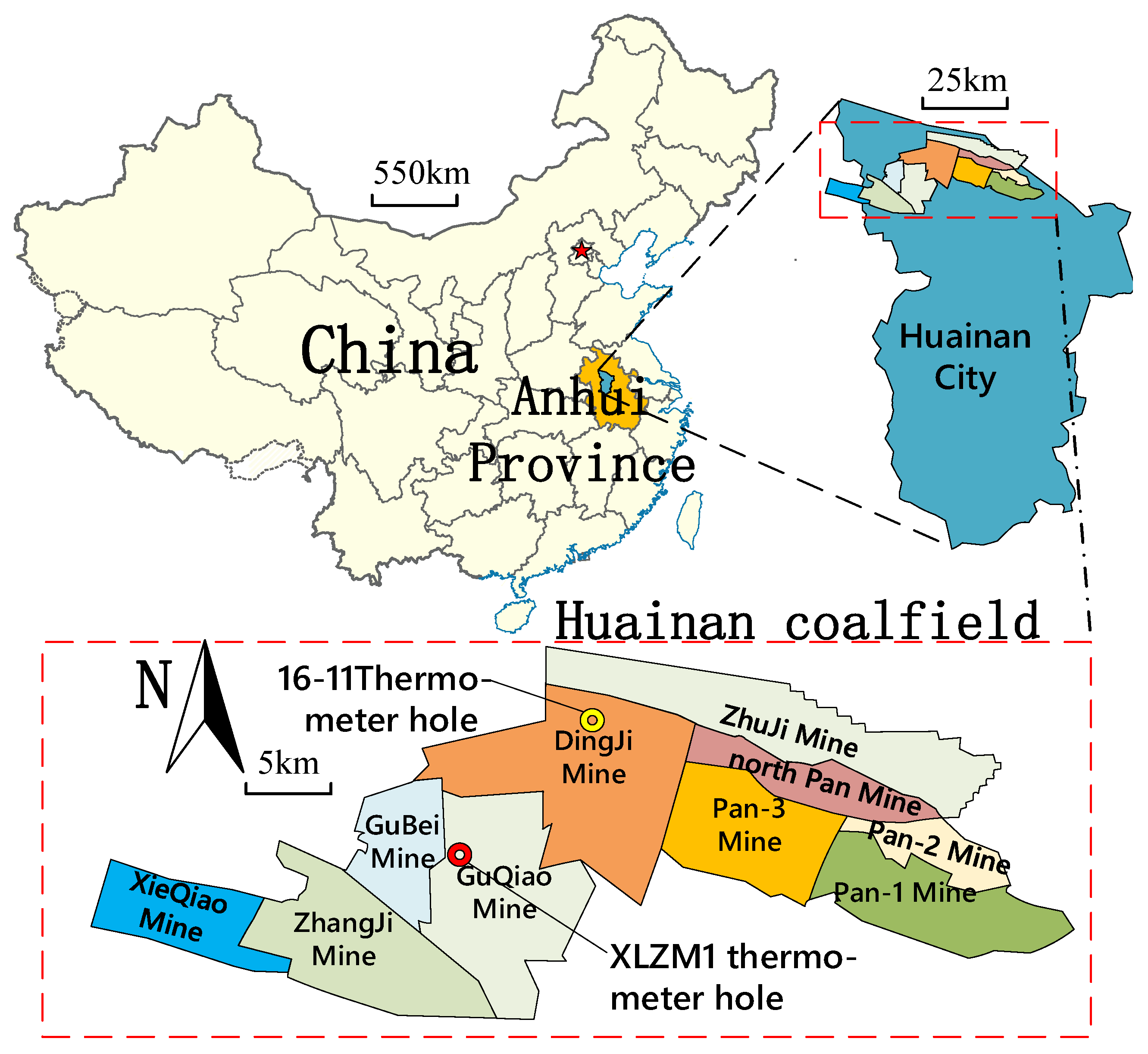
Huainan Coalfield is located in the south of the coal accumulation area in north China, with a length of about 100 km, a width of 20–30 km, and an area of 2500 km², as shown in Figure 5. Strata in Huainan coalfield have typical sedimentary characteristics of a north China platform type. Strata mainly developed from a Lower Proterozoic to Quaternary overlay, but the strata of upper Ordovician O₁ and Upper and Middle Triassic T_1~2 to Middle Jurassic J₂ are missing. The geothermal formation of Huainan Coalfield is closely related to the lithological changes [19,20]. This coalfield, with a total thermal energy reserve of 2.32 × 10¹⁶ kJ, features a wide distribution of thermal energy reserves, even thickness, and uniform lithology. Furthermore, with rich geothermal energy, the coalfield is categorized as a medium–low temperature (II) class and II-3 type stratified geothermal reserve according to the national standard of China (GB/T 1161-2010:3-45) [21].

Guqiao Mine and Dingji Mine (Figure 5) are two mines located in the Panxie mining area of Huainan Coalfield. Many temperature-measuring boreholes have been deployed at each stage of exploration in these two mines, among which the holes XLZM1 and 16-11 are located to the west of Guqiao Mine and to the north of Dingji Mine, respectively. According to exploration data of the geothermal resources, there are abundant geothermal water resources in the Huainan Coalfield below the buried depth of −600 m. The data measured within the buried depth z intervals of (−800 m, −1500 m) and (−600 m, −1020 m) of the two boreholes were taken as the research data. The XLZM1 hole penetrates the Permian, Carboniferous, Ordovician, and Cambrian strata, among which the main aquifers are Cambrian, Ordovician, and Carboniferous. The 16-11 hole penetrates Permian and Carboniferous strata, the latter of which is the main aquifer.

Table 3. Thickness and thermal conductivity of the strata at two temperature-measuring boreholes.

(A) Hole XLZM1 at Guqiao Mine
Formation	Permian							Carboniferous		Ordovician		Cambrian
Thickness (m)	40	18	31	24	18	27	57	31	70	46	18	38	90	85	107
Thermal conductivity	1.95	1.81	1.92	1.98	1.95	2.25	1.71	1.40	2.23	2.35	1.45	2.34	2.34	2.35	2.34
(B) Hole 16-11 at Dingji Mine
Formation	Permian									Carboniferous
Thickness (m)	46		51	38	45	12	42	24	30	33			99
Thermal conductivity	2.80		2.75	1.92	1.80	1.82	1.80	1.95	1.75	1.30			2.35

shows the specifics of these strata.

The parameters of elevation and temperature of the upper and lower boundaries of the two boreholes, porosity, fluid density, and specific heat capacity of the aquifer are shown in

Table 4. Other parameters of the strata and the aquifer at the two temperature-measuring holes.

	Location	Upper Boundary		Lower Boundary		Aquifer
Boreholes		Elevation H0 (m)	Temperature T0 (°C)	Elevation Hn (m)	Temperature Tn (°C)	Porosity n	Fluid Density ρ (kg/m3)	Specific Heat Capacity Cw (J/(kg·°C))
XLZM1		−800	41.8	−1500	61.1	0.13	1000	4200
16-11		−600	34.9	−1020	50.5	0.12	1000	4200

.

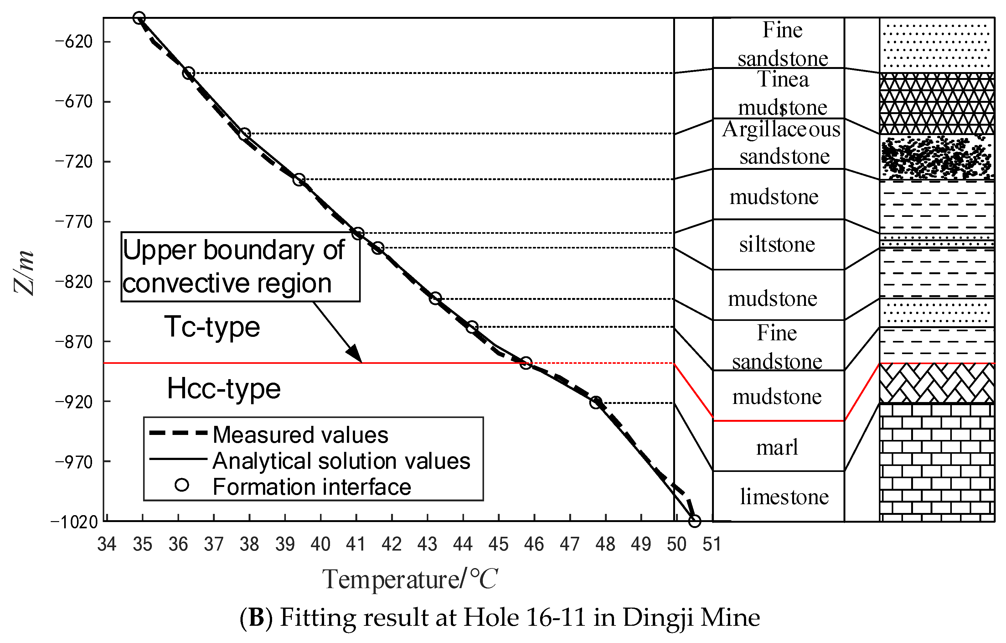
All the known parameters presented in Table 3 and Table 4 were put into the model for calculation, and the calculation results were compared with the measured results. Given the lithology histogram and measured geo-temperature curve of the formation at these two boreholes, it was confirmed that there are both upper Tc-type and lower Tcc-type temperature fields in the study interval.

By adjusting the elevation of the boundary between the two temperature fields and the velocity and direction of groundwater seepage in the Tcc-type region, we fitted the analytical solution curve and the measured geothermal curve. The elevation value of the boundary between groundwater seepage velocity and temperature field of each aquifer is shown in

Table 5. Location and seepage velocity in the Tcc-type region.

	Aquifer	Seepage Velocity (m3/s)			Interface Elevation (m)
Boreholes		Carboniferous	Ordovician	Cambrian
XLZM1		−0.70 × 10−8	−1.35 × 10−8	−0.60 × 10−8	−1020
16-11		−0.75 × 10−8	/	/	−890

. The corresponding fitting of the analytical solution of geothermal curve with the measured value is shown in Figure 6.

As Figure 6 shows, Tc-type and Tcc-type regions are both present in the rock strata at the two boreholes XLZM1 and 16-11. The interfaces of the two regions are shown in the figure. Above the interface, the geothermal temperature curves are inclined straight lines, and the temperature field type is the Tc-type; below the interface, the geothermal temperature curves are convex, the temperature field type is the Tcc-type, and vertical geothermal water occurs in the area. The fitting result revealed that the difference between the measured value and the calculated value was less than 0.2 °C, indicating high goodness of fit and that the value of groundwater seepage velocity was set reasonably. In summary, geothermal water exists in the strata of both boreholes, with buried depths ranging from −1020 m to −1500 m and from −890 m to −1020 m, respectively. Geothermal water migrates vertically upward. The vertical seepage velocity of groundwater in the Carboniferous, Ordovician, and Cambrian aquifers at Guqiao Mine was 0.7 × 10⁻⁸ m³/s, 1.35 × 10⁻⁸ m³/s, and 0.60 × 10⁻⁸ m³/s, respectively, and that at the Carboniferous aquifer of Dingji Mine was 0.75 × 10⁻⁸ m³/s.

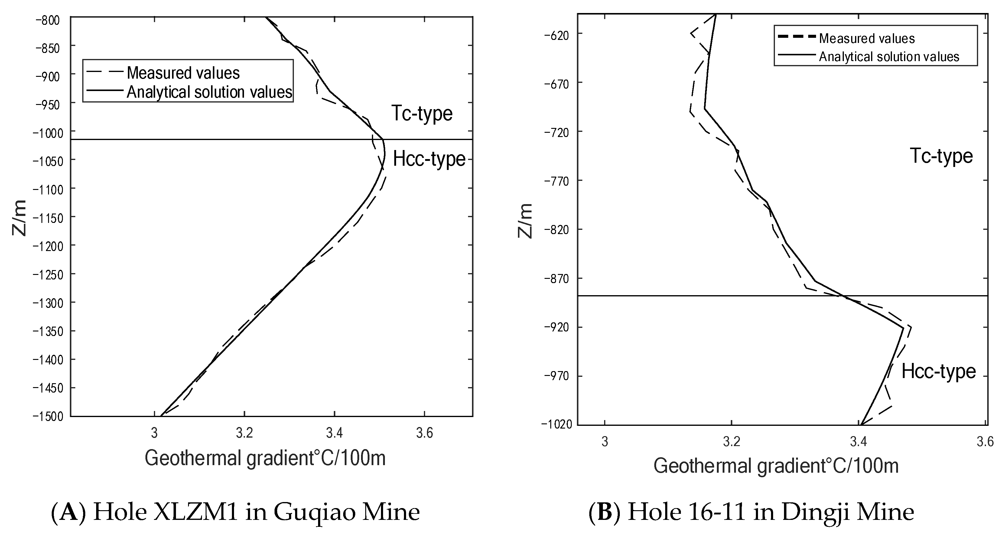
Regarding the geothermal gradient, the geothermal gradient obtained by modeling and the measured gradient were compared [22,23]. As Figure 7 shows, affected by vertical groundwater seepage, the geothermal gradient curves of the two boreholes first increased and then decreased with the increase in buried depth z, indicating the presence of vertical and upward migration of geothermal water in both mines. The variation trend of the geothermal gradient obtained by modeling was nearly the same as that of the measured gradient, and the maximum error was only 0.03 °C/100 m, indicating the high accuracy of the proposed model in reverse-calculating the seepage velocity of groundwater and identifying the occurrence of geothermal water.

5. Conclusions

On the basis of the one-dimensional heat conduction–convection equation, a thermal effect model of vertical groundwater migration in the stratified rock mass was established, and the equations for temperature distribution in stratified rock mass were deduced. The proposed model was employed to analyze the impact of thermal conductivity of the surrounding rocks and the groundwater seepage velocity on the temperature distribution in geo-formations. Furthermore, the model was applied for identification of the parameters of the temperature curve at two temperature-measuring boreholes in coal mines. The following conclusions were drawn:

(1)

The calculation equations for ground temperature distribution in layered strata were derived, which could be employed to calculate the variation of ground temperature caused by vertical seepage of geothermal water and the thermal conductivity of surrounding rocks at any location under the actual geological formations. The parameters required in the calculation equations are easily accessible, and the calculation results are highly accurate as the equations fully consider the factors in actual scenarios.

(2)

In the present work, the geothermal heat transfer patterns in the Tc-type and Tcc-type strata in stratified rock masses were summarized. In the Tc-type strata, the ground temperature was mainly affected by the thermal conductivity of the rock; higher thermal conductivity of the rock led to smaller variations of the ground temperature, while lower conductivity led to larger variations of the ground temperature, and the temperature curve resembled a broken line. In the Tcc-type-type strata, the ground temperature was mainly subject to the vertical seepage of geothermal water; the ground temperature curve was convex when the seepage was upward, but concave when the seepage was downward, and the curvature of the curve grew as the seepage velocity increased. In addition, different from the homogeneous model in which the ground temperature curves were straight lines, the layered model fully showed the geothermal variations caused by the difference of thermal conductivity of the rock mass.

(3)

Application of the model to a study case showed that the difference between ground temperature obtained by modeling and the measured temperature was less than 0.2 °C, the maximum geothermal gradient error was only 0.03 °C/100 m, and the curve fitting degree was high, indicating that the geothermal transfer model of stratified rock masses proposed in this study can appropriately identify the Tc-type and Tcc-type regions in the temperature curve in actual stratified formations. Moreover, the groundwater seepage velocity in the Tcc-type region can be obtained by reverse calculation. The research result is envisioned to provide a geological basis for further development of geothermal water resources.

References

- Cao, Y.F. Geothermal will become a competitive new energy. Chin. Energy 2015, 11, 102–105. [Google Scholar]
- Li, T.L.; Zhu, J.L.; Xin, S.L.; Zhang, W. A novel geothermal system combined power generation, gathering heat tracing, heating/domestic hot water and oil recovery in an oilfield. Geothermics 2014, 51, 388–396. [Google Scholar] [CrossRef]
- Li, T.L.; Liu, Q.H.; Xu, Y.; Dong, Z.X.; Meng, N.; Jia, Y.N.; Qin, H.S. Techno-economic performance of multi-generation energy system driven by associated mixture of oil and geothermal water for oilfield in high water cut. Geothermics 2021, 89, 101991. [Google Scholar] [CrossRef]
- Pang, Z.H.; Luo, J.; Cheng, Y.Z.; Duan, Z.F.; Tian, J.; Kong, Y.L.; Li, Y.M.; Hu, S.B.; Wang, J.Y. Evaluation of geological conditions for deep geothermal energy exploitation in China. Chin. Geosci. Front. 2020, 27, 134–151. [Google Scholar]
- Jaeger, J.K.; Carslaw, H.S. Conduction of Heat in Solids, 2nd ed.; Oxford Press: London, UK, 1959. [Google Scholar]
- Bredehoeft, J.D.; Papadopulos, I.S. Rates of vertical groundwater movement estimated from the Earth’s thermal profile. Water Resour. Res. 1965, 1, 325–328. [Google Scholar] [CrossRef]
- Sorey, M. Measurement of vertical groundwater velocity from temperature profiles in wells. Water Resour. Res. 1971, 7, 963–970. [Google Scholar] [CrossRef]
- Bodvarsson, G.S.; Benson, S.M.; Witherspoon, P.A. Theory of the development of geothermal systems charged by vertical faults. J. Geophys. Res. Solid Earth 1982, 87, 9317–9328. [Google Scholar] [CrossRef] [Green Version]
- Application of Finite Element Method in Geothermal Research; Institute of Geology, Chinese Academy of Sciences: Beijing, China, 1984.
- Lu, N.; Ge, S.M. Effect of horizontal heat and fluid flow on the vertical temperature distribution in a semiconfining layer. Water Resour. Res. 1996, 32, 1449–1453. [Google Scholar] [CrossRef]
- Xu, H.H.; Xiong, L.P.; Wang, J.Y. Study on mathematical Model of thermal effect of vertical fluid migration. Chin. Geol. Rev. 2000, 46 (Suppl. 1), 266–268. [Google Scholar]
- Liu, C.J.; Chen, J.S.; Bai, L.L.; Dong, H.Z.; Chen, L. Calculation and Distribution characteristics of vertical permeability Coefficient of thermal conductivity—Convection type temperature field in fractured rock mass. Chin. J. Rock Mech. Eng. 2007, 4, 780–786. [Google Scholar]
- Gong, H.; Zhu, C.Q.; Xu, M.; Guo, T.L.; Yuan, Y.S.; Lu, Q.Z.; Hu, S.B. The direction of underground water flow and oil and gas storage Conditions based on the temperature measurement curve of drilling—A case study of Dingshan No.1 well in southeastern Sichuan. Chin. Geol. Sci. 2010, 45, 853–862. [Google Scholar]
- Lv, X.; Liu, Y. Characteristics of geothermal distribution and its influencing factors in an jiazhuang well field. Chin. Coal Technol. 2020, 39, 105–108. [Google Scholar]
- Wang, Z.T.; Zhang, C.; Jiang, G.Z.; Hu, J.; Tang, X.C.; Hu, S.B. Current Geothermal field characteristics and genesis mechanism in Xiongan New Area. Chin. J. Earth Phys. 2019, 62, 4313–4322. [Google Scholar]
- Wu, J.W.; Wang, G.T.; Zhai, X.R.; Zhang, W.Y.; Peng, T.; Bi, Y.S. Geothermal characteristics and geothermal resource evaluation in Huainan mining area. Chin. J. Coal Sci. 2019, 44, 2566–2578. [Google Scholar]
- Xu, Y.M.; Hao, W.H.; Fang, S.Q.; Cheng, L.Q.; Du, L.X.; Xie, W.; Nie, C.G. Characteristics and genesis of four geothermal anomalies in Hebei province. Chin. Geol. Bull. 2020, 1–15. Available online: https://kns.cnki.net/kcms/detail/11.4648.P.20201112.1015.002.html (accessed on 6 March 2021).
- Chen, M.X.; Zhang, J.M.; Xia, S.G. Finite element Simulation and case study of the relationship between wellhead water temperature and thermal reservoir temperature. Chin. J. Geosci. 1991, 26, 55–65. [Google Scholar]
- Pan, G.L. Characteristics and prospective zoning of geothermal resources in anhui province. Chin. J. Geol. Disasters Prev. 2011, 22, 130–134. [Google Scholar]
- Wu, H.Q.; Yang, Z.D.; Shu, S.; Cao, H. Geothermal resources distribution characteristics and suggestions for exploitation and utilization in Anhui province. Chin. J. Geol. 2016, 40, 171–177. [Google Scholar]
- Standardization Administration of the People’s Republic of China. Geological Prospecting Criteria for Geothermal Resources (GB/T 11615—2010); Standard Press of China: Beijing, China, 2010; pp. 3–45. [Google Scholar]
- Sun, Z.X.; Zhang, W.; Hu, B.Q. Features of heatflow and the geothermal field of the Qinshui Basin. Chin. J. Geophys. 2006, 49, 130–134. [Google Scholar] [CrossRef]
- Zhang, P.; Wang, L.S.; Liu, S.W. Geothermal field in the South Huabei Basins. Chin. Prog. Geophys. 2007, 22, 604–608. [Google Scholar]
Figure 1.
Temperature field model of a stratified rock mass.
Figure 2.
Temperature–z curves under different seepage conditions.
Figure 3.
Geothermal gradient–buried depth (z) curves under different seepage conditions.
Figure 4.
Temperature–buried depth (z) curves under different schemes of rock thermal conductivity.
Figure 5.
Location of Huainan Coalfield and the distribution of temperature-measuring boreholes.
Figure 6.
Fitting of curves for the calculated temperature and the measured temperature at the two temperature-measuring boreholes: (A) Hole XLZM1 in Guqiao Mine & (B) Hole 16-11 in Dingji Mine
Figure 7.
Fitting of the modeled geothermal gradient curve with the curve of measured data at the two boreholes: (A) Hole XLZM1 in Guqiao Mine & (B) Hole 16-11 in Dingji Mine.