1. Introduction
Vulnerability maps have been widely used for groundwater management, planning, and protection [
1,
2,
3,
4]. These maps are normally based on several geological and hydrological factors. This includes the type of geology, hydraulic properties, and aquifer media, among other things. Some approaches combine the intrinsic properties with other factors, such as contamination load and land-use. Generally, vulnerability maps can be classified into three categories: weighted overlay, statistical methods, and modeling-based methods.
The weighted overlay methods produce the intrinsic vulnerability of a groundwater system based on its physical/hydrogeological properties [
5,
6,
7]. The statistical approach uses statistical tools, such as regression analysis and prediction tools, to build the groundwater vulnerability based on various contaminants and environmental factors [
8,
9,
10]. Modeling-based vulnerability methods use flow and solute transport models to produce vulnerability maps, and, in some cases, are combined with land-use [
11,
12,
13]. Some studies incorporate climate change modeling results in vulnerability assessment [
14,
15,
16].
DRASTIC method (and its many variants) is one of the most widely used index–based approaches for groundwater vulnerability mapping [
17,
18,
19]. This approach relies on the fact that contaminants leach down into aquifers from the land surface and the hydrogeological settings of aquifers may provide some sort of resistance or protection against contaminants [
20]. As such, DRASTIC considers seven factors to create a vulnerability map of groundwater. These factors are depth to the water table, net groundwater recharge, aquifer media, soil media, land slope, the impact of the vadose zone, and hydraulic conductivities [
20].
DRASTIC approach (and all index-based methods) classifies each factor and applies specific ratings for each category. It also assigns standard weights for each factor. Then it sums up all weighted classes to produce the final vulnerability index. While the original developed DRASTIC uses specific rates and weights, various studies adopted localized rates and weights. The classifications of parameters and the assigned weights may vary from one study to another, as there are no clear rules for the rating and weights selection. The rating classification may significantly affect the resulting vulnerability.
Fuzzy Logic (FL) is one of the artificial intelligence tools that mimic human reasoning. In the Boolean logic of computers, only two possibilities are available: yes or no (0,1). FL allows for a degree of contribution to the answer, which is represented by a membership function, as explained later. It has been widely used in hydrogeology. Nobre et al. [
21] used fuzzy hierarchy to evaluate groundwater contamination risk in Brazil. They combined fuzzy logic with numerical model and DRASTIC vulnerability to produce a risk index. Nadiri et al. [
22] used fuzzy logic to analyze and model time series of groundwater levels. Another study used fuzzy logic to create variogram for spatial analysis of groundwater level interpolation [
23], which found to improve the results. Other studies combined fuzzy logic with other tools for groundwater assessment [
24], groundwater pollution level [
25], and groundwater quality [
26]. FL is advantageous as it considers the degree of the truth (not the probability). It deals with possibilities based on set theory. For example, a certain contaminant in groundwater may or may not exceed the maximum permissible limit, based on crisp analysis. FL enables assigning a degree of exceedance of the maximum permissible limit. In addition, FL overcomes the problem of the boundary between categories in the classical vulnerability assessment methods. Because vulnerability thematic maps may contain high uncertainty, FL is more suitable than the classical index–methods.
This study produces an FL-based groundwater vulnerability map for Qatar and compares it with a DRASTIC-based index-based one. To have a fair comparison, a solute transport model for the study area was developed and used to validate the vulnerability results of both methods. Results were checked against actual anthropogenic–sourced contamination.
2. Materials and Methods
The following sub-sections describe the study area and the methods followed for vulnerability mapping, groundwater modeling, and validation. The study area describes the main hydrogeological settings and groundwater status, and the vulnerability sub–section describes DRASTIC method. The last part of this section describes fuzzy logic, membership functions, and overlays method. Results of both DRASTIC and fuzzy logic vulnerability are checked against groundwater model, and the comparison is presented in the discussion part.
2.1. The Study Area
Qatar is a small country located in the eastern part of the Arabian Peninsula and covers an area of around 11,500 km
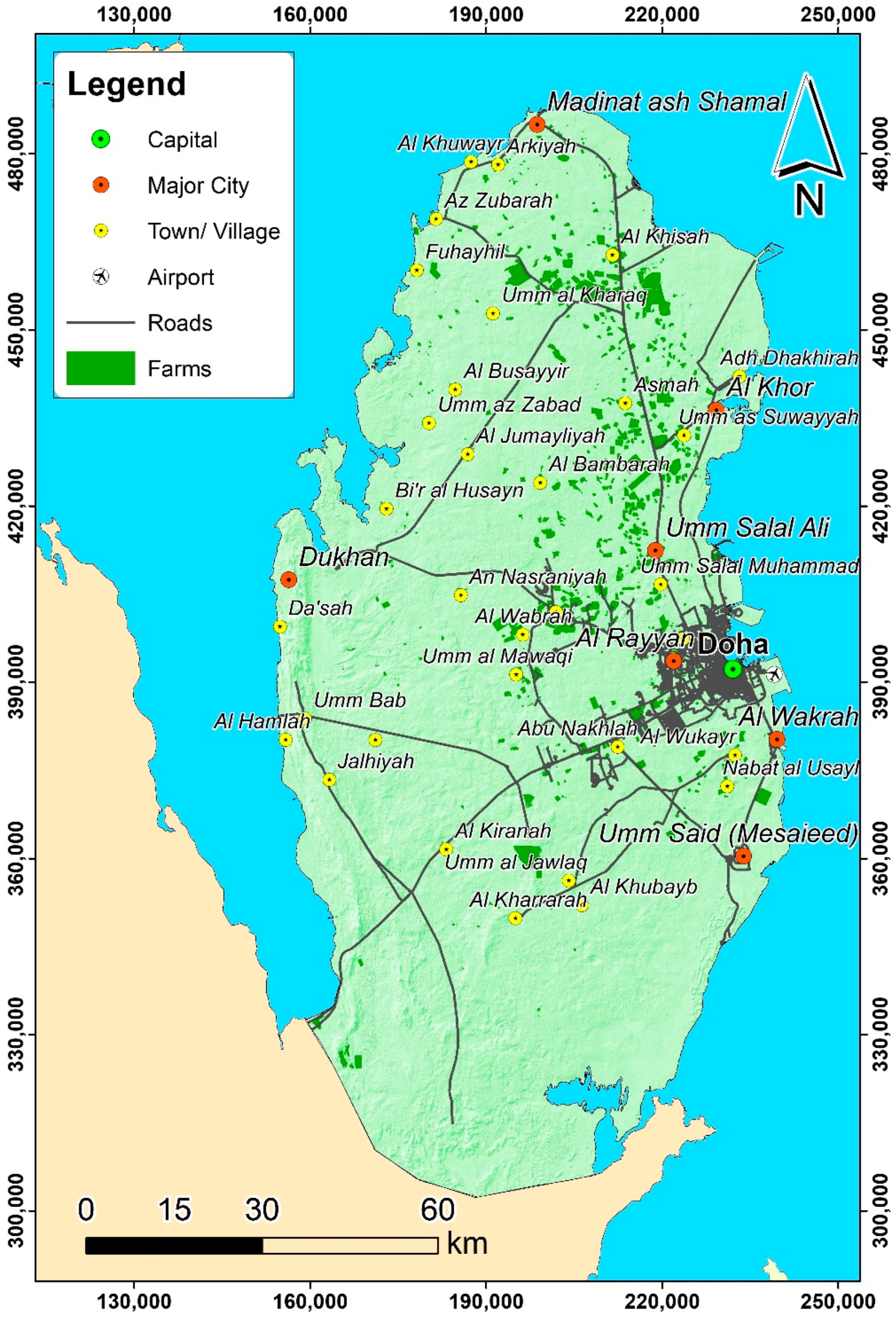
2. It is surrounded by the Arabian Gulf from all directions except for the south, where it has a boundary with Saudi Arabia (
Figure 1). The terrain of the country is flat, except for some small areas in the south, but the topography altitude varies between 0 near the coast to around 107 m above mean sea level inland [
4]. The country has a population of around 2.8 million inhabitants (as of 2021). Aquifers are the only natural source of water, which is almost solely used for irrigation. Domestic and industrial demand is met by desalination plants. The average annual groundwater abstraction is 250 million m
3 [
27]. Farms, especially in the northern part of the country (
Figure 1), are the main consumer of groundwater. Aquifer recharge is very little due to low rainfall and harsh climate conditions. The annual average rainfall is no more than 80 mm [
28,
29], and the long-term annual recharge is around 60 million m
3 [
4,
30,
31]. As a result of this substantial overexploitation, groundwater level has dramatically dropped over the last few decades, resulting in serious environmental problems. These problems include loss of aquifer storage, the salinity of groundwater increases, and seawater interface advanced further inland.
The surface geology of Qatar comprises mainly carbonate formations, with some Quaternary deposits, such as sand dune and beach sediments. Tertiary formations from the middle and early Eocene make the main aquifer in Qatar. The uppermost main three layers are from top to bottom: Dam & Dammam Formation, Rus Formation, and Umm Er Radhuma Formation, respectively [
28,
29,
30]. They have a variable thickness, but Rus and Umm Er Radhuma are the main aquifers. These layers comprise mainly limestone and dolomite, with some clay layers in various places, and gypsum deposits, especially in the southern part of the country. Groundwater level varies between 0 near the coastal areas to around 10 m above mean sea level in the middle of the aquifer. Dam & Dammam Formations are dry, except for the coastal areas. Rus and Umm Er Radhuma are the two main aquifers. Rus aquifer is being recharged locally by rainfall, whereas Umm Er Radhuma received its water from regional flow infiltrates the formation outcrop in Eastern Arabia [
29,
31,
32].
The groundwater quality is relatively good in the north, compared to the southern part, where it is saline. This is because of the dissolution of gypsum formation that occurs in the southern part of the country, in addition to the higher recharge that the northern aquifer receives. Because of overexploitation of groundwater resources in Qatar over the last few decades, the quality has significantly deteriorated. Other environmental impacts include seawater intrusion and upconing of brackish deep groundwater.
Data used in this study come from various sources. Surface and subsurface geology data came from published reports and journal papers, in addition to interpretation of structural contours [
28,
33]. The soil data, classification, and soil map are based on the Atlas of soil Qatar [
34]. Depth to water table was calculated using piezometric survey data [
21]. Aquifer recharge was based on previous studies [
24,
27,
31,
35].
Hydraulic properties were based on aquifer test data [
27], and calibrated model results [
28]. Groundwater recharge data came from various sources [
31,
35]. Topography data are based on LiDAR (or light detection and ranging) data from the Ministry of Municipalities and Environment in Qatar. A digital elevation model was created in GIS, and the slope function of Spatial Analyst was used to create the slope map.
2.2. DRASTIC Vulnerability
Aller et al. [
20] were the first to propose DRASTIC approach for groundwater vulnerability. DRASTIC assumes contaminants move to groundwater from land surface and hydrogeological settings of the aquifer provide some sort of protection against contamination. The acronym DRASTIC represents seven parameters. These are: depth to water table/confining layer, net recharge, aquifer media, soil media, topography, impact of vadose zone, and hydraulic conductivities. Numerous studies have used DARSTIC and its variations to build groundwater vulnerability maps [
36].
DRASTIC vulnerability index is given by [
20]:
where D, R, A, S, T, I, C are the seven DRASTIC parameters mentioned before, and the subscript r indicates the rate. The numbers multiplied by these parameters are the standard weights by Aller et al. [
20]. The DRASTIC model has been used and applied in many areas around the world, with various hydrological and climate settings. Climate impact on DRASTIC results depends on how extreme all relevant parameters are. In arid countries, net recharge is small, whereas depth to the water table is high, compared to wet countries. This provides higher vulnerability in arid countries, but other parameters, such as aquifer, topography, and soil media, play an important role.
2.3. Fuzzy Logic Analysis
Fuzzy Logic was first proposed by Zadeh in 1965 as an alternative to the 0–1 Boolean approach [
37]. Unlike weighted overlay approaches, Fuzzy logic allows more flexibility in rating than the classical weighted overlay methods. As such, instead of assigning specific classes as in DRASTIC, with specified boundaries, fuzzy Logic assigns a continuous membership value varies between 0 and 1, using a certain function that can be identified as a prior (membership function). Weights are not important in fuzzy overlay, as it is based on set theory and not linear combination.
The membership function shows how likely a parameter is a member of a set. It should be noted that the membership function is about the possibility and not the probability. For example, if the hydraulic conductivity of an aquifer varies between 10 and 30 m/day, the membership function of the hydraulic conductivity will transform class values to be between 0 and 1 [
38]. The higher value of the membership function (i.e., 1) the more likelihood the class contribution will be. Several membership functions exist [
39]. The most common ones are: The available functions are fuzzy Gaussian, fuzzy Large, fuzzy Linear, fuzzy MSLarge, fuzzy MSSmall, fuzzy Near, and fuzzy Small.
2.3.1. Fuzzy Gaussian
Fuzzy Gaussian is derived from the probability density function as the most likelihood occurs in the center and values with less likelihood occurs at either side of the function.
The transformation function for Fuzzy Gaussian membership is:
where f
1 and f
2 are the spread and the midpoint, respectively. Fuzzy Gaussian membership function is not suitable for vulnerability mapping.
2.3.2. Fuzzy Large
Fuzzy large membership function is used when large values increase the contribution to the membership. For example, the larger value of hydraulic conductivity increases the latter contribution to vulnerability. Thus, Fuzzy Large may be used in to produce the membership function of hydraulic conductivity. In the standard Fuzzy Large function, the default midpoint is 0.5. The transformation to Fuzzy Large is given by:
where f
1 is the spread, and f
2 is the midpoint.
2.3.3. Fuzzy MS Large
This is like Fuzzy Large where the contribution to the membership function increases directly, but the difference is the MS Large uses the mean and the standard deviation. High fuzzy memberships take values above the mean in this case. The membership function of Fuzzy MS Large is given by:
where m and s are the mean and the standard deviation of the variable, respectively, and a and b are multiplier for the mean and the standard deviation, respectively. The resultant membership function takes a sigmoid shape with the mean membership value is 0.5. Equation (4) above is valid when a × m < x. If a°m ≥ x then µ(x) = 0.
2.3.4. Fuzzy Small
Fuzzy Small is the inverse of Fuzzy Large. That is, the higher value of the variable corresponds to lower contribution to the membership function. High fuzzy memberships take values below the mean in this case. For example, higher depth to water table decreases the contribution to vulnerability; thus, Fuzzy Small can be used to represent it.
where f
1 is the spread, and f
2 is the mean of the input variable.
2.3.5. Fuzzy MS Small
This is the inverse to Fuzzy MS Large:
Equation (6) above is valid when a × m < x. If a × m ≥ x, then µ(x) = 0. All variables are as previously defined.
2.3.6. Fuzzy Linear
This function is used when a variable is linearly increases or decreases. The equation of this membership takes the following from if the variable contribution is increasing:
where max and min are the maximum and the minimum values of the variable, respectively.
If the variable contribution is decreasing, then the membership is:
3. Results
3.1. DRASTIC Vulnerability
DRASTIC model was done in GIS using Equation (1). Seven thematic maps were prepared in ArcGIS, based on previous studies and modeling work [
4,
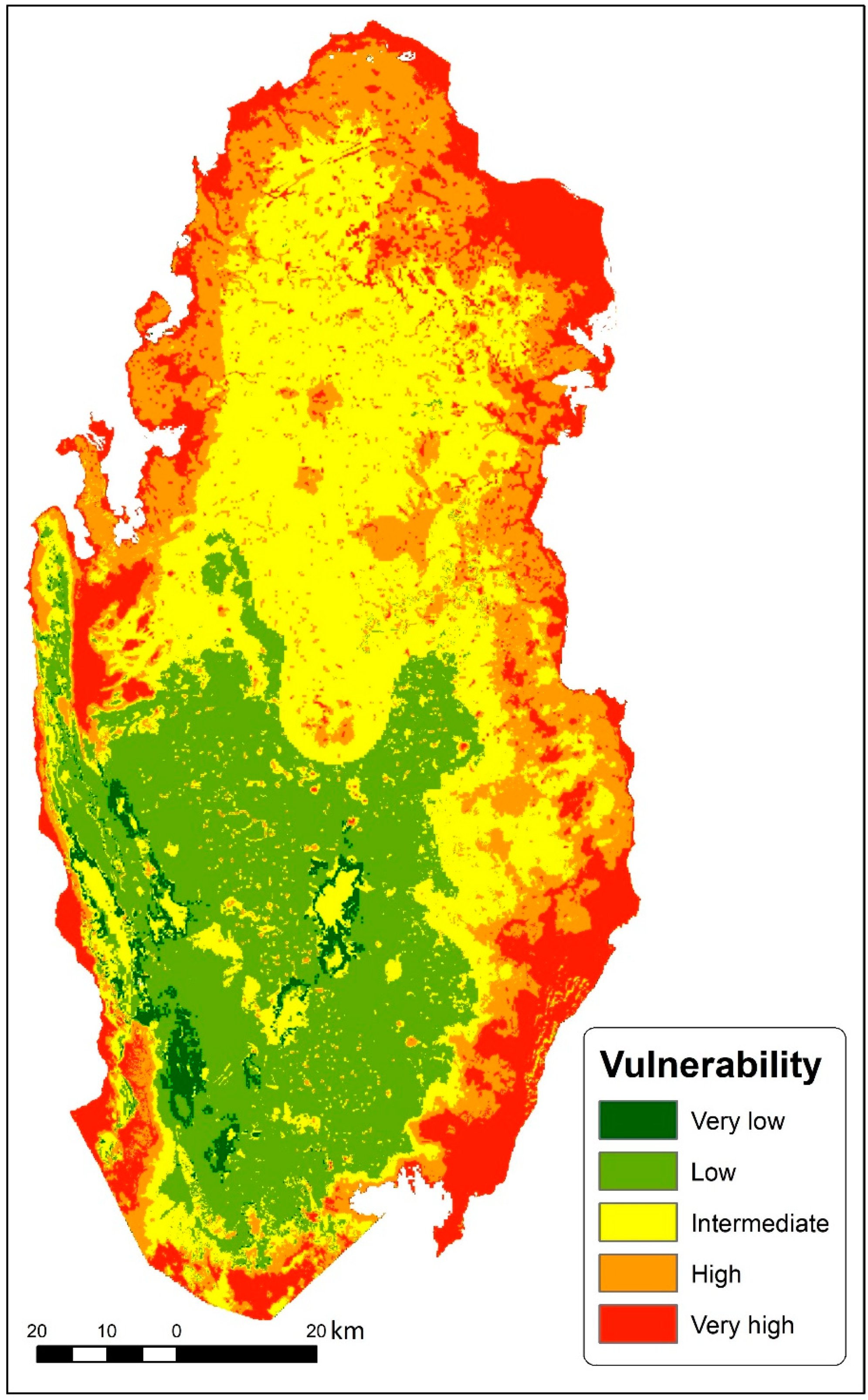
28], and the resulting DRASTIC vulnerability map is shown in
Figure 2. The map was classified into 5 categories (very low, low, intermediate, high, and very high).
The resulting vulnerability map shows the majority of Qatar falls under low to intermediate class, whereas the high vulnerability areas occur along the coastline. This is because the coastal areas have low terrain, and the depth to water table is small. DRASTIC assigns the highest weight for depth to water table, which explains why these areas have high vulnerability.
3.2. Fuzzy Logic Vulnerability
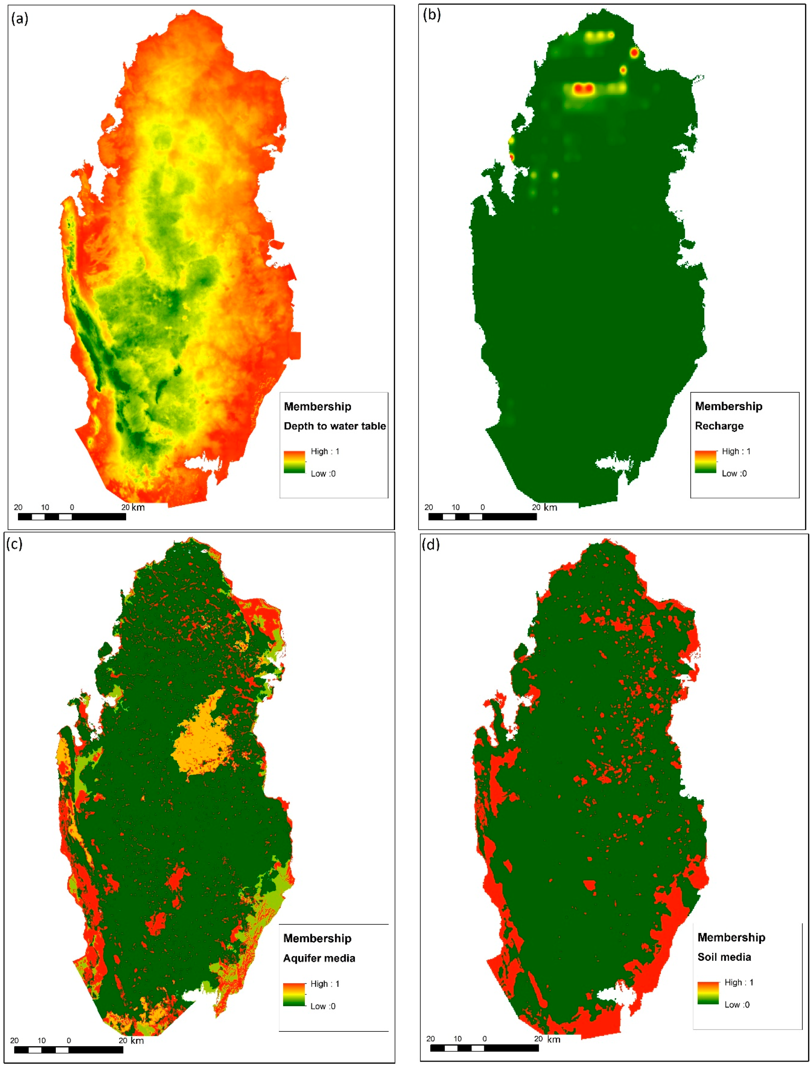
Based on the previous discussion, the linear membership functions were used to convert the seven parameters of DRASTIC approach to fuzzy membership. All variables used increasing linear trend except for depth to water table, and topography (i.e., slope), where the membership contributions are indirectly proportional to variable increase (linear decreasing trend). Using ArcGIS, the membership functions of the seven thematic maps were produced, as depicted in
Figure 3. Values of various parameters were obtained based on previous studies [
4,
34,
35].
Fuzzy Overlay (FO) enables identify the relation between membership sets. It provides more flexibility than the traditional weighted overlay [
40]. In the case of vulnerability assessment, FO takes the effect of all parameters into consideration and produces the overlay map, which has class values between 0 and 1. Several Overlay functions are available in ArcGIS. These are: And, Or, Product, Sum, and Gamma [
41,
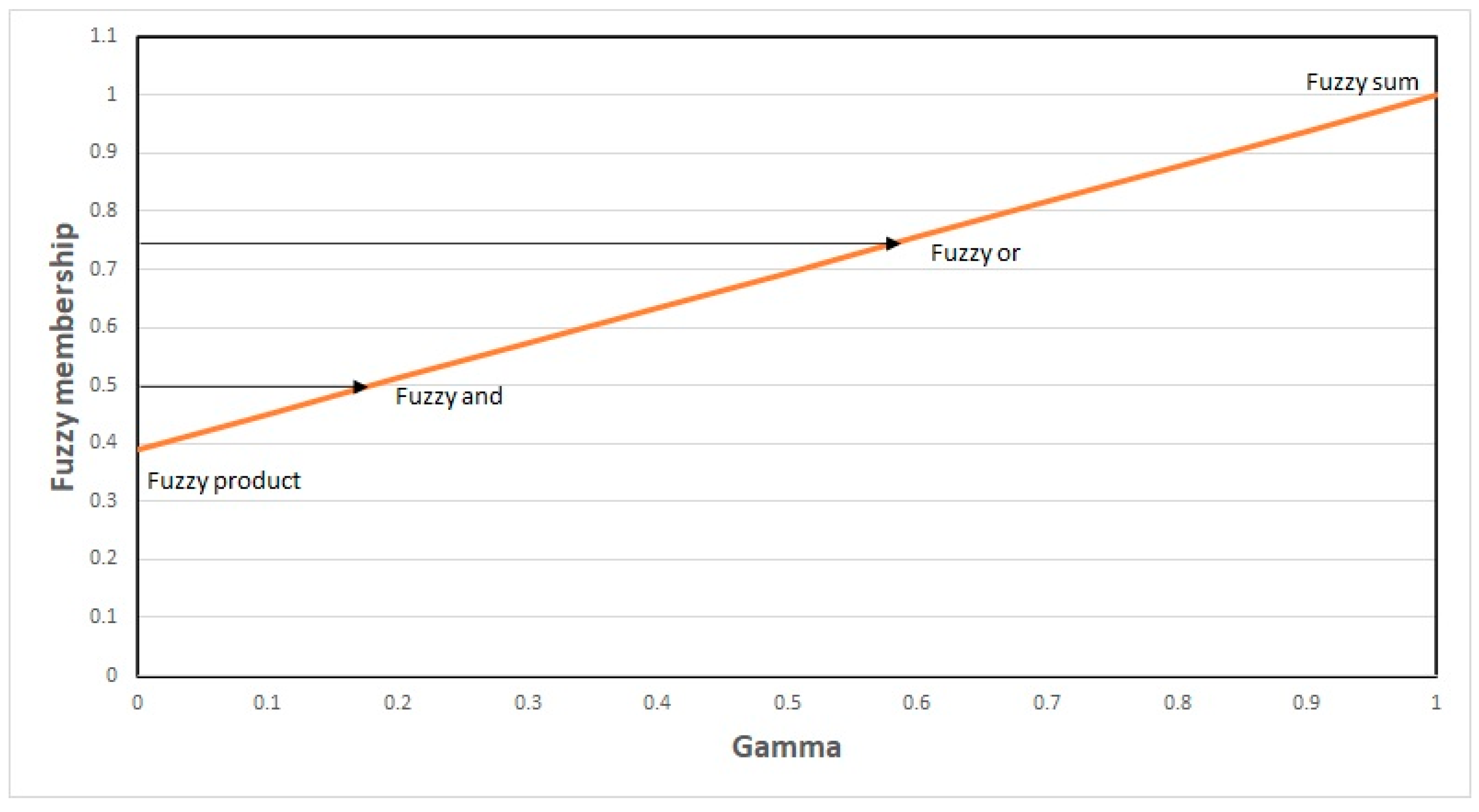
42]. The overlay “Fuzzy And” produces the minimum value of the cell, contrary to “Fuzzy OR”, which returns the maximum value of the cell from all layers. Overlay “Fuzzy Product” produces the product of all values in a cell from all layers. The overlay “Sum” is algebraic sum and not additive. It is a linear increase of fuzzy values at a cell. “Gamma” is a special type produces a value between Fuzzy Product and Fuzzy Sum.
Table 1 below summarizes the various FO available in ArcGIS, and how each overlay is calculated.
Figure 4 shows the relationship between Gamma value and Fuzzy membership functions. If Gamma = 0, then the membership equals Fuzzy product. When Gamma is 1, then the membership is Fuzzy sum. “Fuzzy and” and “Fuzzy or” are in between.
DRASTIC map (
Figure 2), FL vulnerability map shows higher variability, and more skewed towards high vulnerability.
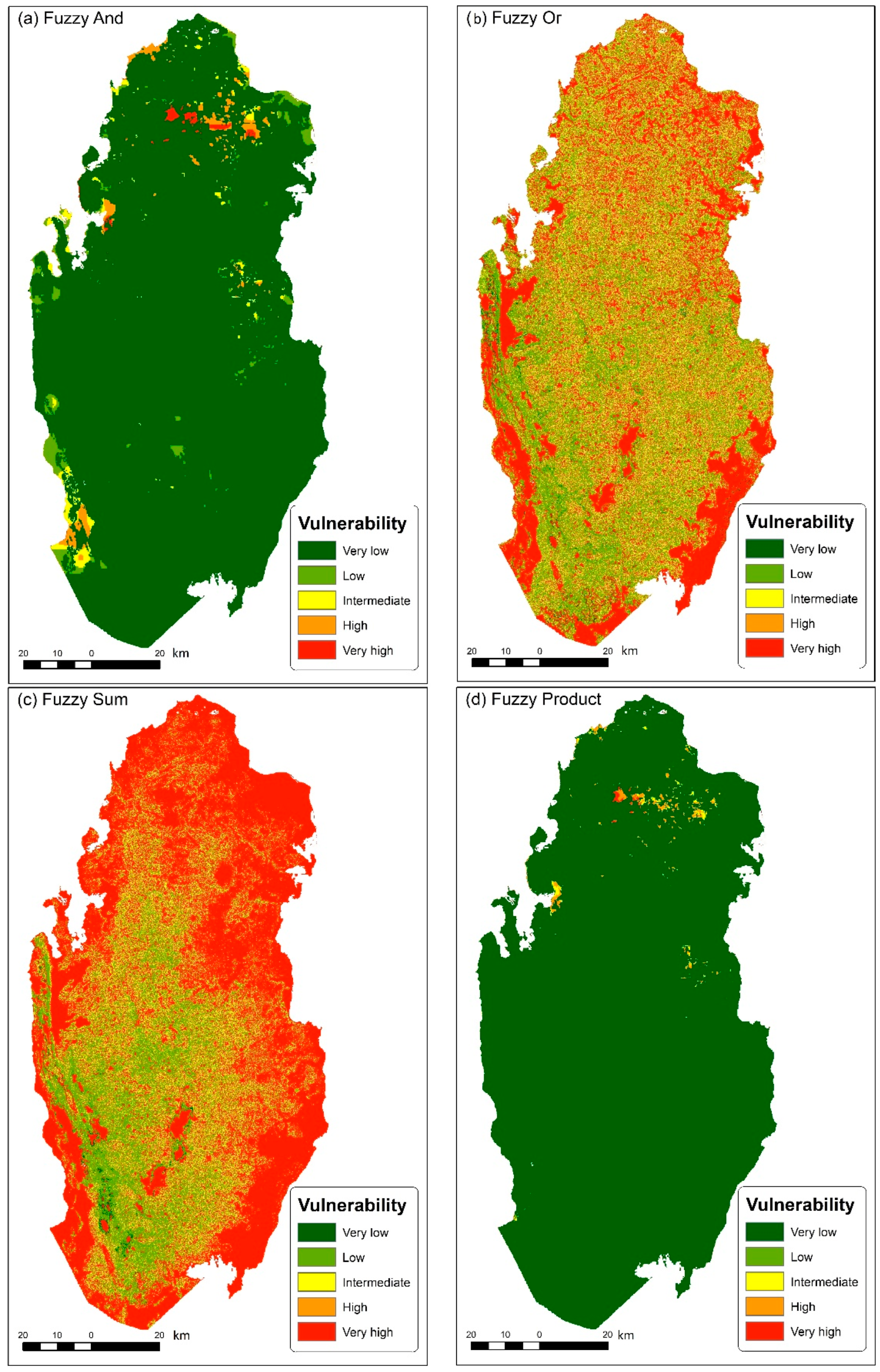
Using the Spatial Analyst tool of ArcGIS, various fuzzy overlays were used to produce the vulnerability map based on fuzzified variables, as shown in
Figure 5. Vulnerability maps vary significantly based on the overlay method.
Fuzzy And is on the lower side of membership, as most of the produced map occurs in the very low vulnerability. Fuzzy Or is a sort of intermediate (it corresponds to 75% of the membership, as shown in
Figure 5b). The high vulnerability areas occur only along the coastal areas in the southern part of the country. This is also not reflecting the actual vulnerability as most of the area occurs in the intermediate class. Fuzzy Sum (
Figure 5c) shows a more plausible distribution of vulnerability classes, with high vulnerability along the coast and some inland areas in the north. Fuzzy Product (
Figure 5d) is at the lowest end of vulnerability classification, so it is not representative.
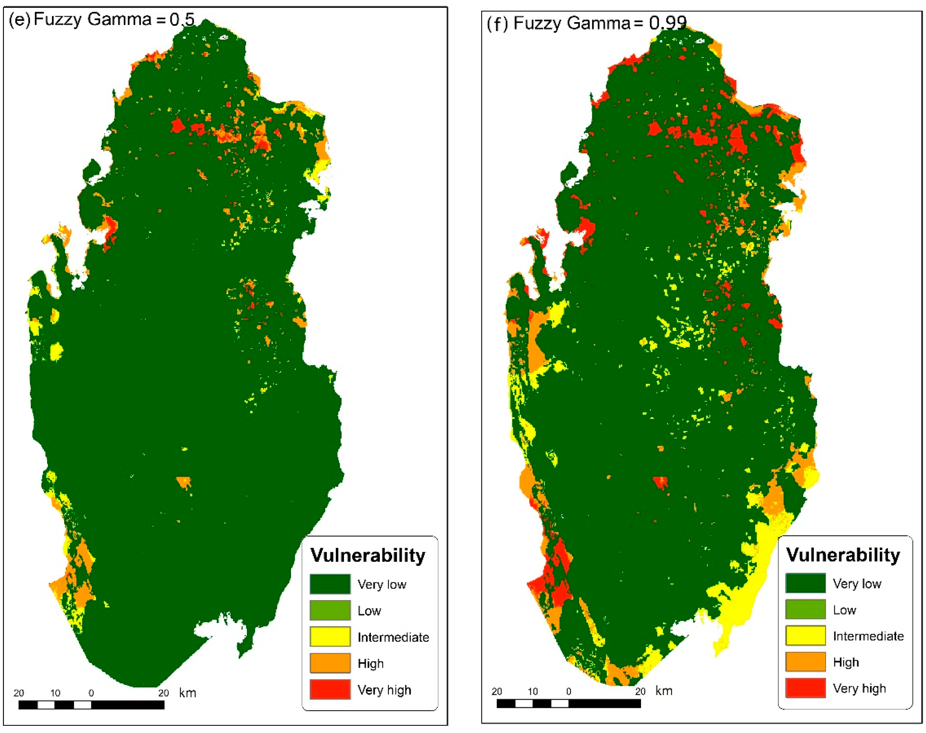
Figure 5e shows the Fuzzy Gamma= 0.5, which is mostly in the very low vulnerability, whereas Fuzzy Gamma = 0.99 is shown in
Figure 5f. The latter shows a more plausible distribution of vulnerability classes. In this study, Fuzzy Sum and Fuzzy Gamma = 0.99 will be considered and compared to DRASTIC, as they show a better distribution of vulnerability and less skewness.
3.3. Comparison with Groundwater Model Result
To check the validity of both vulnerability models, a 3D groundwater flow model and solute transport were developed. The model is based on the finite–difference MODFLOW, covering the entire country of Qatar, with a 500 × 500 m grid size. Data for the model was based on the previously published work of [
34], and the model was calibrated for steady-state conditions.
The model includes three layers representing the main geological formations in the country: Dam & Dammam, Rus, and Umm Er–Radhuma formations. The steady-state model was calibrated against field measurements.
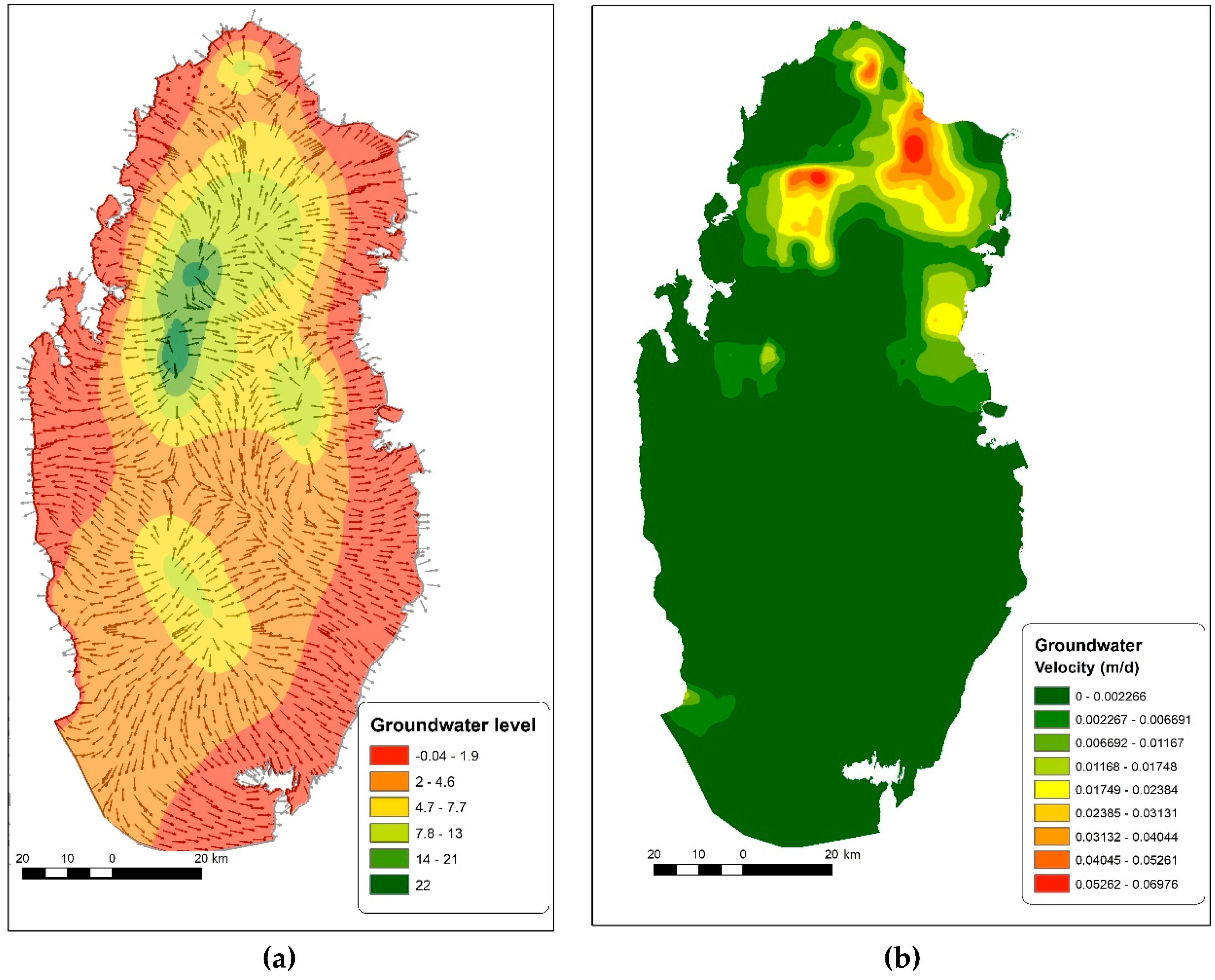
Figure 6 shows the simulated groundwater level contours for the steady–state simulation, and the velocity magnitude. The level map resembles the pre-development conditions of water resources. Groundwater levels vary between 0 near the sea to more than 22 m above mean sea level in the middle of the northern aquifer. The velocity vectors are also shown in
Figure 6, which indicate the flow direction.
Modeling results reveal that the coastal areas are a discharge zone for groundwater. This implies any solute or contaminant flow with the mobility of water will end up in these areas.
On the other hand, the middle of the aquifer (groundwater mound) is a recharge area where flows originate. Despite being located upstream, these areas are in the low vulnerability class due to the high depth to groundwater.
The groundwater velocity magnitude shows the highest velocities occur in the northern and north–eastern parts of the country. Areas of high groundwater velocity are more vulnerable to contamination because high velocity enables fast movement and more distribution of contaminates when introduced in these areas. When draping velocity map (
Figure 6) over FL Sum, FL Gamma = 0.99 maps (
Figure 5), and DRASTIC map (
Figure 2), some match is observed between high velocity and high vulnerability. The area of mismatch is the high velocity over the middle of the north aquifer. FL Sum shows the best match with velocity map, compared to DRASTIC or FL Gamma.
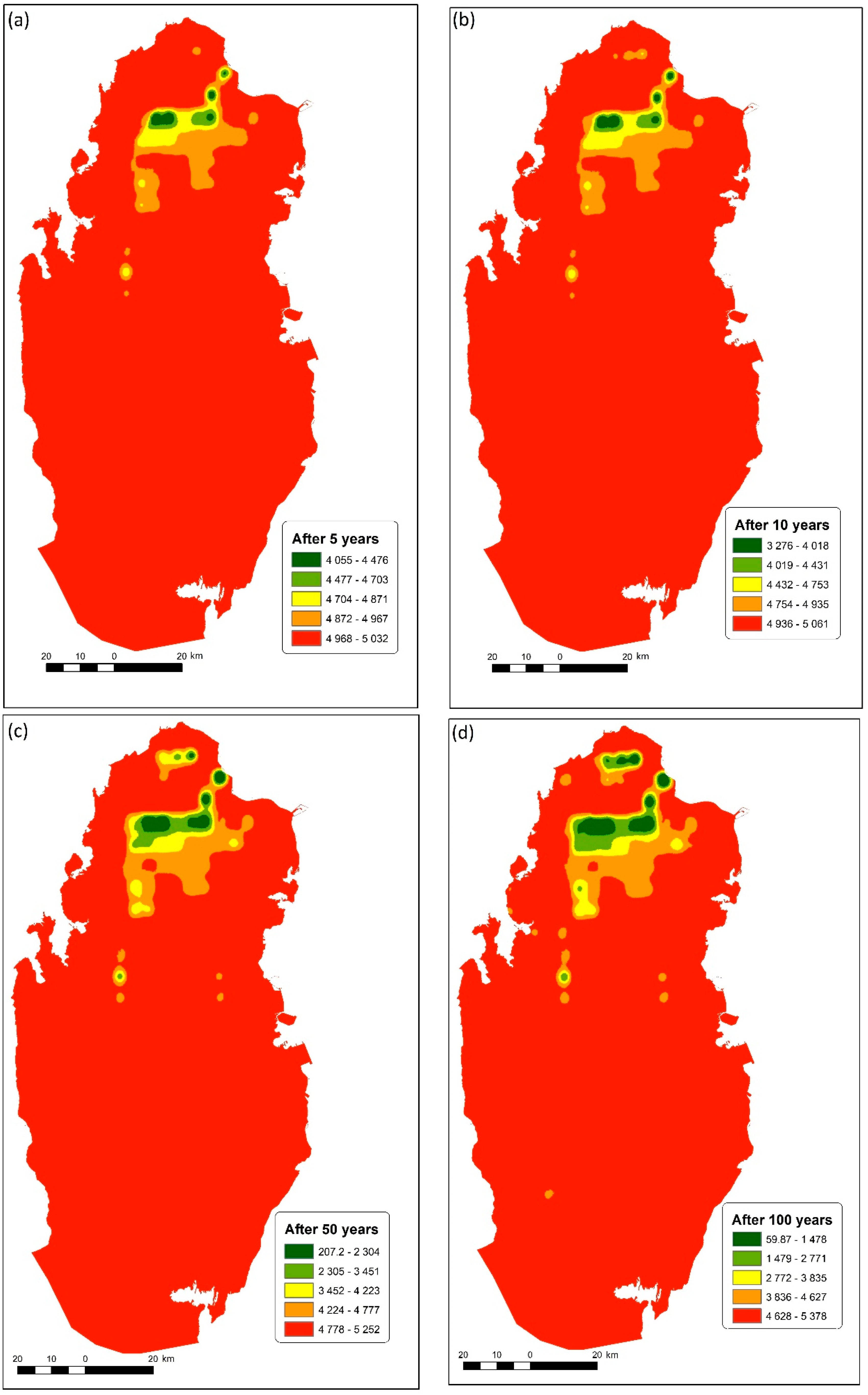
A solute transport model was developed using MT3DMS [
43]. The velocity matrix from the flow model was used to run the solute transport model. Advection and dispersion components were considered in the model, and an equal and homogeneously distributed initial concentration of total dissolved solids (TDS) = 5000 mg/L was introduced at the beginning of the simulation. The model was run for 100 years.
Figure 7 shows the propagation of the solute at 5, 10, 50, and 100 years. Like the velocity magnitude, the concentration decreases in the northern area of the model and increases elsewhere. This is another indication of the high vulnerability of the northern area, in addition to some smaller areas in the middle of the country.
It should be noted that vulnerability may not necessarily reflect the actual contamination load in aquifers. This is because a source of contamination must exist on land surface of a vulnerable area for contamination to occur [
44]. Like velocity, solute transport propagation appears to move faster in the northern part of the country, because of high hydraulic conductivity. These areas are highly vulnerable because any contamination introduced on the land surface will spread fast in the aquifer.
3.4. Chemical Indicators in Aquifer
Qatar General Electricity and Water Corporation (KAHRAMAA) monitors the groundwater state of the environment on regular basis, using a network of wells. The main chemical parameters being analyzed include major ions and cations, in addition to salinity and TDS. The source of these contaminants is mainly natural due to the dissolution of gypsum and other salts in the sub–surface and the nature of limestone geology. As a result, analyzing the concentration of these chemicals is not helpful for vulnerability mapping. This is because intrinsic vulnerability assumes all contaminants come from the land surface and percolate down into the aquifer.
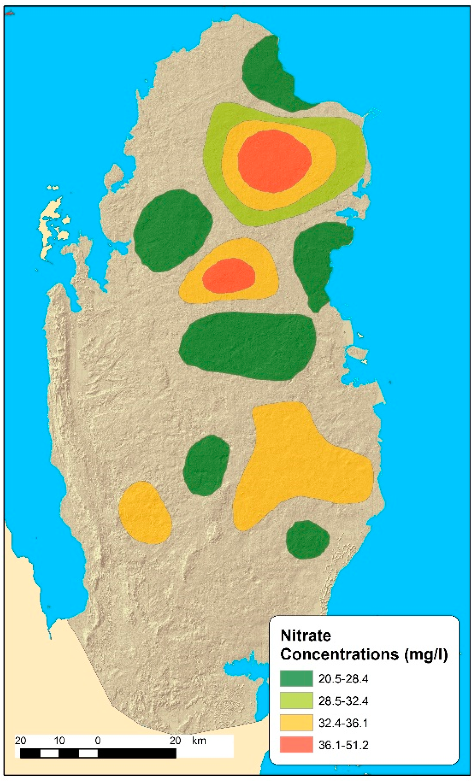
Nitrate contamination in groundwater in Qatar comes mainly from the heavy application of fertilizers, in addition to leachate of wastewater from some ponds (i.e., Abu Nakhla area) [
45]. As such, it may help to look at nitrate concentration and relate it to vulnerability mapping.
Figure 8 shows the main nitrate contamination zones in the groundwater of Qatar, based on Ahmad et al. [
45]. The highest concentrations (50 mg/L) occur in the north–eastern part of the country, which is the maximum permissible limit by the World Health Organization [
46]. This area is known for many agricultural farms, where organic fertilizers are applied heavily [
45]. Some areas in the south show moderate to low nitrate concentration due to leakage from wastewater ponds. It should be noted that most agricultural activities occur in the northern part of the country (
Figure 1), where the fresh groundwater occurs. Besides, most built-up areas are in the eastern side of the country, where wastewater is a major source of nitrate contamination. As such, sources of nitrate contamination do not exist in the west and south-western parts of Qatar.
4. Discussion
This study aimed at exploring the usage of fuzzy logic for vulnerability assessment using Qatar as a case study. Results were compared with DRASTIC method, and both FL and DRASTIC were examined against groundwater model results and anthropogenic impact.
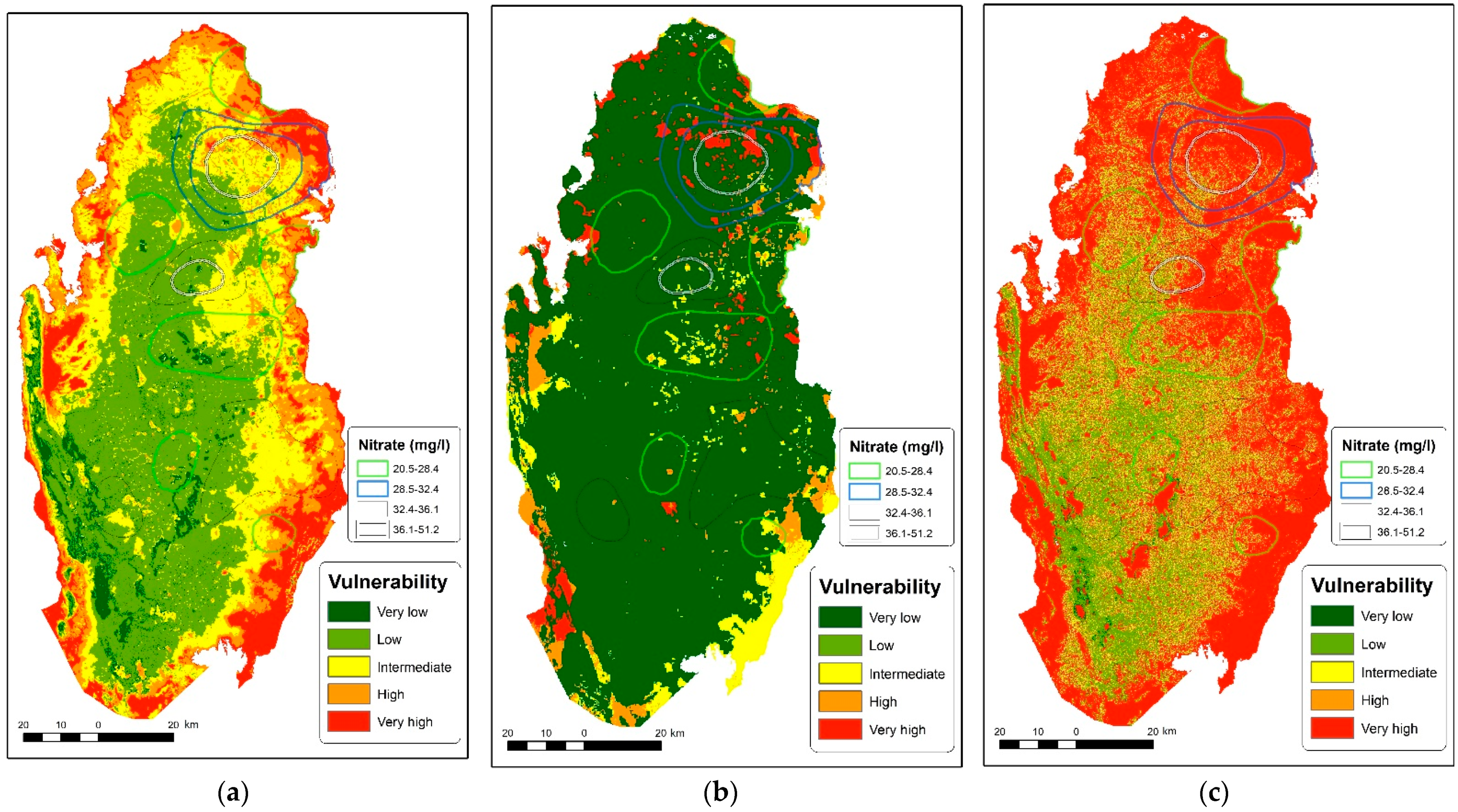
Figure 9 shows a comparison between DRASTIC, FL–Gamma = 0.99, and FL Sum with nitrate contours overlaid each. DRASTIC and FL Sum show the high vulnerability areas are along the coast, but the latter approach includes larger areas in this class than the former. While DRASTIC emphasis more on the depth to the water table, FL has no focus on one single factor. FL map shows a greater interaction between various vulnerability classes, but DRASTIC produces a gradual change between vulnerability levels.
It should be noted that the nitrate concentrations are indicative only. By definition, an area of high vulnerability will become contaminated if a contamination source on land exists [
44]. In other words, some areas can be highly vulnerable despite the aquifer underneath has no contamination because of absent of contamination source. This is the case in the south and in the western parts of Qatar, where no on-land activities, such as agriculture, occur. The highest nitrate concentrations (triple black line closed contour in the figure) occur over the intermediate and low vulnerability classes of DRASTIC. The same contours occur over very high, intermediate, and low vulnerability areas of FL Gamma. In FL Sum, high nitrate contours occur over very high and intermediate vulnerability. The FL Sum has by far a better match with nitrate concentration than DRASTIC and FL–Gamma.
The limitation of this work is the lack of a robust way for comparison of FL and DRASTIC. Although anthropogenic contamination load provides a fair way to check vulnerability, the latter does not necessarily correlate strongly with contamination load. However, this limitation affects both DRASTIC and FL equally, so the comparison is still fair. Future research should focus on exploring various overlay methods of FL to find the most suitable one for vulnerability assessment.
5. Conclusions
Groundwater vulnerability maps are useful for groundwater protection and assessment. Most vulnerability assessment methods revolve around the use of hydrogeological settings, which are assumed to provide a certain level of protection against contamination. The problem with these methods is the use of ad–hoc rating and weights for each hydrogeological parameter to produce the index map, and then to classify the map into various vulnerability classes. Classification of parameters to assign ratings is challenging as there is no robust method to identify the boundary between various bands. Fuzzy Logic (FL) eliminates all these challenges using membership functions, and it does not require weights for input variables.
This study compares vulnerability assessment results of DRASTIC and FL approaches. In absence of any measure of accuracy, the combination of numerical models and actual anthropogenic contamination load is useful to check the results of various vulnerability methods. Results show both DRASTIC and FL produce vulnerability maps with some similarities and some differences. DRASTIC produces a vulnerability map with a gradual change in classes and more homogeneous patterns, whereas FL-based map has a heterogeneous pattern. The coastal areas in both DRASTIC and FL maps occur within the very high vulnerability, but this class extends further inland in the FL. The FL map shows a better agreement with groundwater velocity from the flow model, and the actual contamination load resulting from land-use activities. As such, FL is probably more suitable for vulnerability assessment in this case. However, more research is needed to explore the impact of fuzzy membership variation on the results. In addition, various FL overlays produce significantly different vulnerability maps, which requires further research on this issue. Results of this study revealed Fuzzy Sum is more suitable than other FL overlays methods, although Fuzzy Gamma seems to be promising but requires further research.


