
Evaluation of Subsurface Drip Irrigation Designs in a Soil Profile with a Capillary Barrier


1
Faculty of Agriculture, Tokyo University of Agriculture and Technology, 3-8-1, Harumicho, Fuchu, Tokyo 183-8538, Japan
2
School of Geography and the Environment, University of Oxford, South Parks Road, Oxford OX1 3QY, Oxfordshire, UK
3
Research Center for Biology, Indonesian Institute of Sciences, JlRaya Jakarta-Bogor Km 46 Cibinong, West Java 16911, Indonesia
4
Department of Environmental Sciences, University of California, Riverside, Riverside, CA 92507, USA
*
Author to whom correspondence should be addressed.
Water 2021, 13(9), 1300; https://doi.org/10.3390/w13091300
Submission received: 5 April 2021
/
Revised: 27 April 2021
/
Accepted: 29 April 2021
/
Published: 6 May 2021
(This article belongs to the Special Issue Development and Application of Subsurface Irrigation Techniques)
Abstract
:Enhanced water use efficiency (WUE) is the key to sustainable agriculture in arid regions. The installation of capillary barriers (CB) has been suggested as one of the potential solutions. CB effects are observed between two soil layers with distinctly different soil hydraulic properties. A CB helps retain water in the upper, relatively fine-textured soil layer, suppressing water losses by deep drainage. However, retaining water in a shallow surface layer also intensifies water loss by evaporation. The use of subsurface drip irrigation (SDI) with a CB may prevent such water loss. This study evaluated the performance of SDI in a soil profile with a CB using a pot experiment and numerical analysis with the HYDRUS (2D/3D) software package. The ring-shaped emitter was selected for the SDI system for its low capital expenditures (CapEx) and maintenance. Strawberry was selected as a model plant. The results indicated that the proposed SDI system with a CB was effective in terms of WUE. The numerical analysis revealed that the CB’s depth influences the system’s water balance more than the ring-shaped emitter’s installation depth. While the CB’s shallow installation led to more root water uptake by the strawberry and less water loss by deep drainage, it induced more water loss by evaporation.
1. Introduction
In semi-arid and arid regions, agricultural production is dependent on vulnerable water resources. Water insecurity is expected to intensify in the future due to climate change, such as global warming [1,2]. Predictions suggest that the anticipated increase in evapotranspiration due to rising temperatures may be more significant than the increase in precipitation [3]. The severe effect of water shortages is already apparent in some regions [4]. The development of water-efficient agricultural practices is thus required for sustainable food production.
The installation of Capillary Barriers (CB) has been suggested as a promising engineering approach to improve agricultural water use efficiency (WUE) [5,6,7,8,9,10]. A CB, a natural barrier to unsaturated water flow in soils, can be observed at the boundary of two soils with distinctly different hydraulic properties. When a fine-textured layer overlies a coarse-textured layer, the water in the fine-textured layer does not infiltrate into the coarse-textured layer if the capillary forces in the fine-textured layer are significantly stronger, retaining moisture in the fine-textured layer. This is due to the coarse material having much larger pore sizes. This CB effect is maintained until a certain soil water pressure (breakthrough pressure) is reached at the interface of the two materials. At the breakthrough pressure, the capillary forces of the fine-textured layer match those of the coarse-textured layer so that liquid water can infiltrate from the layer above a CB into the CB layer [11]. CBs have been used for decades to contain and control hazardous wastes [12,13].
Many studies have been dedicated in recent years to the application of CBs to agricultural production. Ityel et al. [5] investigated the effect of introducing a CB layer into surface-irrigated cultivation plots. This study reported that up to 70% more water was retained in the root zone as a result of the CB suppressing downward water drainage, also resulting in reduced water content fluctuations [5]. An increase in the root zone’s water content can be observed regardless of plant types [6,7,8,9]. These changes prevent plants from being exposed to water stress, especially in arid regions. Even though the response to the CB installation varies crop by crop [6], it generally provides positive effects for biomass and/or fruit production [6,7,8].
A downside of CBs is that water loss by evaporation may increase [8,9]. Miyake et al. [8] conducted a cultivation experiment on a leafy vegetable with sprinkler irrigation and showed that a CB might fail to improve root zone conditions when the amount of applied water (AW) is insufficient, as evapotranspiration intensified in the CB’s presence. Wongkaew et al. [9] also reported that water loss by evaporation increased by 8.0–62.3% in a CB’s presence. The HYDRUS-1D simulation of leafy vegetable cultivation with surface irrigation showed that up to 90% of AW was lost by evaporation in the presence of a CB [9]. The increase in water loss by evaporation is likely the result of water retained near the surface, as the soil water content near the soil surface is one of the determinants of the actual evaporation rate [14,15].
One of the potential solutions to intense evaporation is to implement subsurface drip irrigation (SDI). Under SDI, water loss by evaporation is significantly smaller than under surface irrigation, as less water is directly exposed to the atmosphere [16,17]. Despite its drawbacks, such as high capital expenditures (CapEx) and maintenance [16,18,19,20], SDI is widely used in the large-scale production of horticultural crops [18]. Martines and Reca [16] compared the WUE of SDI and surface drip irrigation in olive cultivation. They revealed that 8–20% water saving was achieved by the use of SDI. Bonachela et al. [15] measured the evaporation rate in the olive field production and showed that the evaporation rate could be suppressed by keeping the ground surface dry. O’Brien et al. [18] compared the economic performance of SDI and sprinkler irrigation. They showed that the high WUE of SDI offers an economic advantage, despite its high CapEx and maintenance that may hinder its adaptation by farmers. These past studies indicate that the use of SDI may help overcome the shortcomings of CBs. However, there are no studies investigating the feasibility of SDI when used together with a CB.
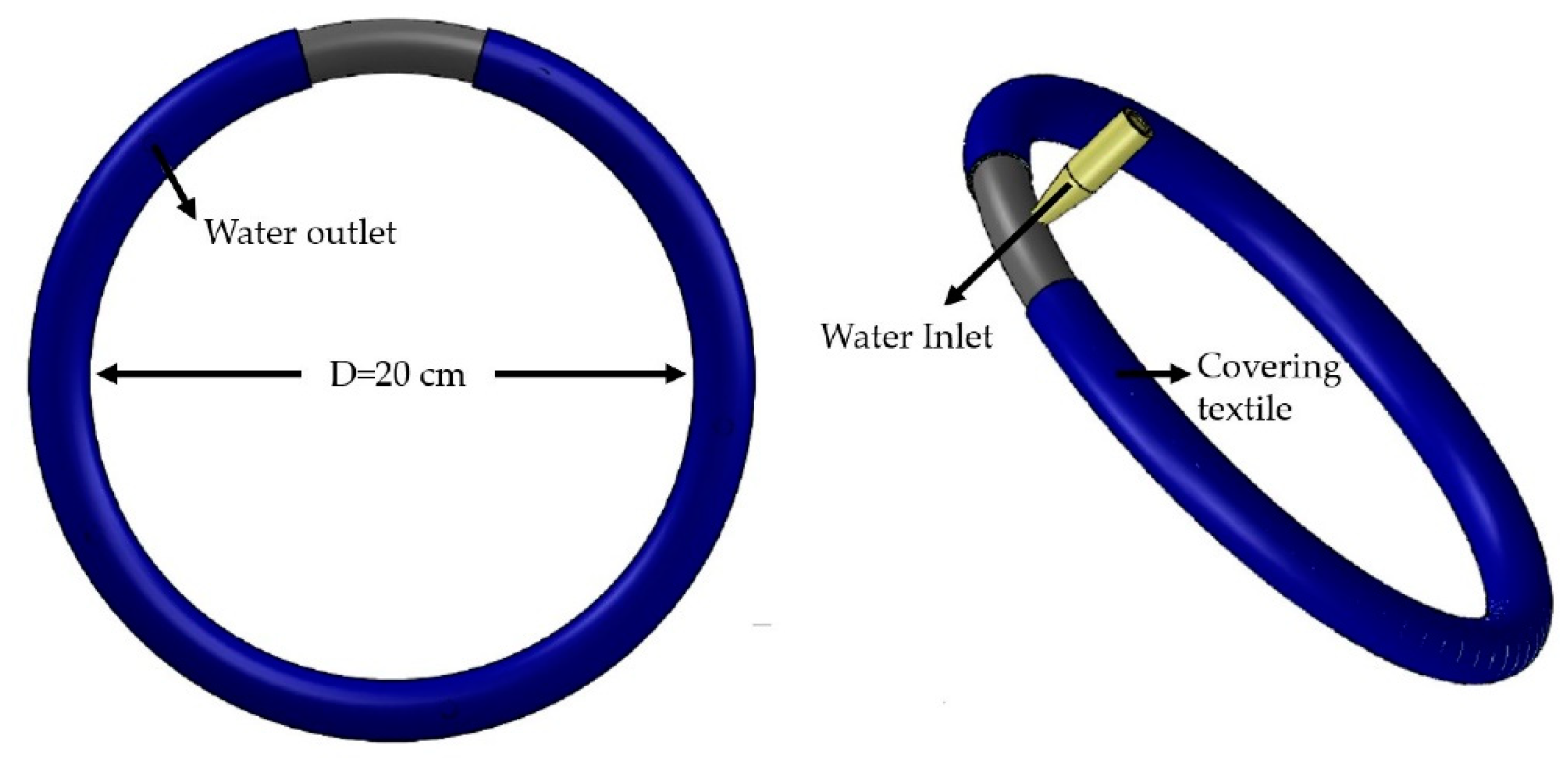
In recent years, to further disseminate SDI by overcoming the aforementioned drawbacks, SDI with ring-shaped emitters (Figure 1) has been extensively studied [17,19,20,21]. Saefuddin and Saito [19], for example, showed that a ring-shaped emitter made of a rubber hose could improve WUE during bell pepper cultivation. In their study, two to five holes were drilled into the ring-shaped rubber hose, through which water was applied [19]. The ring-shaped hose was covered with textile so that water infiltrated in all directions when buried subsurface [19]. The simple design and material of the ring-shaped emitter makes it easy for small-scale low-income farmers to use the emitter in practice [19,20]. The feasibility of the ring-shaped emitter has been confirmed for the field production of various crops [21]. Saefuddin and Saito [19] investigated the effect of the number of holes in the ring-shaped emitter and revealed that the emitter with five holes enabled the highest yield, while the emitter with two holes produced the highest WUE. Saefuddin et al. [20] analyzed the ring-shaped emitter’s performance experimentally and revealed that downward water flow is more dominant than radial flow in the sand profile. Saefuddin et al. [20] further evaluated the ring-shaped emitter’s performance numerically using the HYDRUS (2D/3D) software package. They showed that non-uniformity in the wet volume occurred in the sand profile, putting some roots under water stress. However, the system used in their analysis was relatively simple as the pot was filled uniformly with sand. A more detailed observation of soil water dynamics in a layered soil profile may be needed to further improve the design and operation of SDI with the ring-shaped emitter in practice.
The SDI setups with the ring-shaped emitter were numerically investigated by Friedman and Gamliel [17]. However, it should be noted that a tree was the model plant in their study. Hence, the SDI design (several ring-shaped emitters were placed around the tree) was significantly different from other studies [19,20,21]. The study revealed that the preferable depth of the ring-shaped emitter depends on the evaporation rate. The study reported that a deeper emitter installation depth led to a decrease in root water uptake (RWU) when evaporation was assumed negligible. On the other hand, increasing the ring-shaped emitter’s installation depth to a certain point increased RWU in the presence of intense evaporation. The deepening of the emitter, however, is not always possible. For instance, when a CB layer is installed below the root zone, the emitter’s deep installation may result in the accumulation of water on a CB, which would lead to its breakage and hence water loss by deep percolation. The effects of the SDI emitter’s installation depth and a CB on water loss and RWU need to be investigated in a soil profile with a CB.
To facilitate the development of the SDI design with the ring-shaped emitter, we aimed to evaluate its feasibility in a soil profile with a CB. First, the ring-shaped emitter’s performance in a soil profile with a CB was analyzed both experimentally and numerically. The experimental analysis was conducted using a pot experiment. The numerical analysis was then performed to evaluate effects on the plant water stress and water losses using the HYDRUS (2D/3D) software package [22] with data obtained from the pot experiment and literature. The HYDRUS (2D/3D) software package has been proven to be able to provide accurate predictions of water flow for SDI [20,23,24] and a CB [5,13]. Finally, the effect of changing the installation depth of the ring-shaped emitter and a CB on overall water balance (i.e., RWU, evaporation, and deep drainage) was evaluated using the HYDRUS (2D/3D) software package [22].
2. Materials and Methods
2.1. A Laboratory Experiment with a Ring-Shaped Emitter and a CB
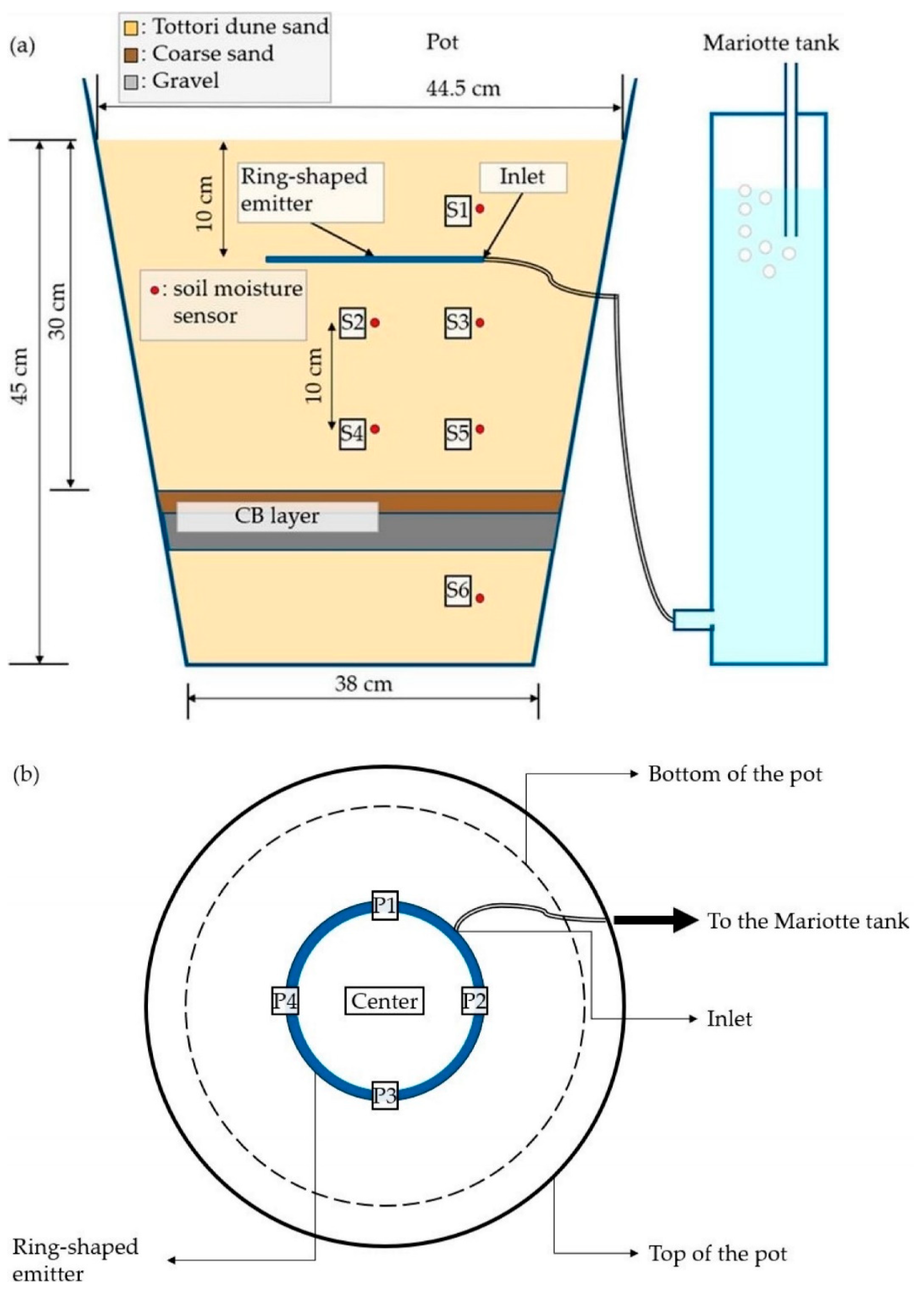
A pot experiment was conducted in a lab using a plastic pot as shown in Figure 2. The temperature in the lab was kept at 24 °C for the entire duration of the experiment. The height of the pot was 55 cm. The pot was first filled with Tottori dune sand from the bottom up to a height of 10 cm. The Tottori dune sand (D50 = 292 µm) had 0.1% of its particles smaller than 75 µm, 0.2% in the range of 75–106 µm, 36.6% in 106–250 µm, 55.2% in 250–425 µm, and 8.0% in 425–850 µm. A two-layered CB layer was then placed upon the Tottori dune sand layer. The CB layer comprised a 3 cm gravel layer (particle diameter > 2 mm) and a 2 cm coarse sand layer (particle diameter range of 0.85–2 mm) overlying the gravel layer. While the gravel layer’s function was to suppress downward water flow as a CB, the coarse sand layer’s role was to prevent small Tottori dune sand particles from falling into the gravel layer and nullifying the CB function [8,9]. A 30 cm Tottori dune sand layer was then placed on the CB layer. The bulk density of all Tottori dune sand layers was adjusted uniformly at a predetermined bulk density of 1.50 g cm−3. The pot’s diameters at the sand layer’s height (45 cm from the bottom) and the bottom were 44.5 cm and 38 cm, respectively. All three materials were oven-dried at 105 °C for at least 24 hours before the experiment.
A ring-shaped emitter with a diameter of 20 cm was placed 20 cm above the CB layer to inject water into the Tottori dune sand profile. The ring-shaped emitter had five evenly spaced holes (water outlets), all facing downwards. The holes were covered with a permeable textile, following the 5F design of Saefuddin and Saito [19]. Water was injected every 24 hours by applying a constant water pressure head of 0 cm at the inlet connected to a Mariotte tank. A total of 1080 cm3 of water was injected during each water application cycle. The amount of water supplied during each water application cycle was determined based on the strawberry’s typical potential transpiration rate (=720 cm3) [20]. The injected water was then left to redistribute in the soil profile for the rest of the 24 hours. This water application process was repeated 16 times in the pot experiment (i.e., the pot experiment continued for 16 days). The time required for each water application was recorded manually. The recorded water application time was used to calculate the water flux values at the emitter surface in the inverse estimation of soil hydraulic properties (See Section 2.2).
Soil water dynamics were monitored using six soil moisture sensors installed in the Tottori dune sand layers. The red dots in Figure 2a show the positions of the soil moisture sensors. The soil water content was recorded every 10 minutes using the EM50 probes (METER Environment) and the MIJ-01 datalogger (Environmental Management Japan). The EM50 soil moisture sensor, a standard capacitance sensor, measures soil dielectric characteristics, which are further used to estimate soil volumetric water contents. In this study, a calibration equation provided by the METER Environment was used because it is known that this calibration equation performs well for sands.
After Day 16, core samples of the gravel, coarse sand, and Tottori dune sand were collected at a 5 cm interval to measure the volumetric water content gravimetrically. At each depth, five soil samples from five different horizontal positions (depicted as P1, P2, P3, P4, and center in Figure 2b) were collected to reveal the horizontal water content distribution. It should be noted that the inlet of the ring-shaped emitter was between P1 and P2. The collected samples were oven-dried at 105 C for at least 24 hours to measure the volumetric water content.
2.2. The HYDRUS (2D/3D) Inverse Estimation of Soil Hydraulic Parameters and Simulation of the Pot Experiment
Some of the Tottori dune sand’s soil hydraulic parameters were optimized using the inverse solution of HYDRUS (2D/3D). The HYDRUS (2D/3D) software package [22] simulates soil water dynamics in a two-dimensional, three-dimensional, and axisymmetric domain by solving the Richards equation with a source/sink term S(h):
where θ(h) denotes the volumetric water content [-], h is the soil water pressure head [L], t is time [T], S(h) signifies a sink term [T−1], K(h) is the unsaturated hydraulic conductivity function [L T−1], and x, y, and z are the axes of the Cartesian coordinate system [L]. The sink term S(h) represents RWU.
The parameters were optimized by minimizing an objective function, which expresses discrepancies between observed data and simulated results. The objective function is first calculated using the initial parameter estimates. The parameters are then iteratively modified so that the objective function is minimized. The iteration process continues until a predetermined precision is achieved. More details about the parameter estimation method can be found in the technical manual of HYDRUS (2D/3D) [25].
The authors attempted to conduct the inverse parameter estimation in a fully three-dimensional domain. However, the calculation stopped before the parameters were optimized due to computational instability. For this reason, the inverse estimation of soil hydraulic parameters and the simulation of the pot experiment were conducted in an axisymmetric domain. This axisymmetric modeling approach has been adopted in many other studies on SDI (e.g., [20,26,27]). The simulation domain was finally discretized into 1390 nodes and 2664 two-dimensional elements. The finite element mesh around the ring-shaped emitter was made fine to stabilize the computation of HYDRUS (2D/3D).
The solution of the Richards equation requires an appropriate soil water retention curve model and initial and boundary conditions. In coarse materials such as coarse sand and gravel, non-capillary-type flow occurs after water is drained quickly by capillary flow [9]. A dual-porosity (DP) model may be more appropriate than single-porosity (SP) models to describe such soils’ soil hydraulic properties. Brunetti et al. [28] statistically evaluated the accuracy of the Durner [29] model, a DP model, in comparison to the van Genuchten [30] model, a typical SP model. They reported that the use of the Durner [29] model led to more accurate predictions of volumetric water contents (VWC) and the K(h) function of a coarse material, especially in the dry range (4 < log|h| < 6) and near saturation. The use of the SP model resulted in an unrealistically small estimation of K(h) even in a relatively high soil water pressure range [28]. Wongkaew et al. [9] also compared the predictive accuracy of the soil hydraulic conductivity function for coarse sand and gravel using the van Genuchten [30] and Durner [29] models, revealing that the Durner [29] model showed a better agreement with measured data. Based on these studies’ findings, the Durner [29] model shown below was used in this study Equation (2,3):
where Se1 and Se2 are effective water contents [-], θr and θs are the residual and saturated water contents [-], respectively, w1 and w2 are the weighting factors for two overlapping regions with different water retention characteristics, respectively, and Ks is the saturated hydraulic conductivity [L T−1]. Parameters α1, α2 [L−1], m1, m2, n1, and n2 [-] are the fitting parameters. Initial estimates of soil hydraulic parameters of each soil are presented in Table 1. It should be noted that the van Genuchten [30] model was applied for Tottori dune sand by setting the w2 value to zero.
The parameters for the coarse sand and gravel obtained by Wongkaew et al. [9], which were estimated by the inverse solution of HYDRUS-1D [31], were adopted. The saturated hydraulic conductivity Ks and the saturated water content θs of the Tottori dune sand were measured by the constant-head permeability test and gravimetrical measurement, respectively. The θr value was determined based on the initial soil water content recorded in the pot experiment. Finally, the values of α, l, and n were estimated by the HYDRUS (2D/3D) inverse solution.
The initial VWC of the soil profile was set to 0.02 based on the measured data in the pot experiment. No-flux boundary condition was applied to the bottom and sides of the pot. An atmospheric boundary condition with an observed potential evaporation rate of 1.36 mm d−1 was applied at the soil surface. A time-variable flux boundary condition was assigned as a boundary condition at the ring-shaped emitter. As the rate of water application was known from the pot experiment, the water flux values at the emitter surface were determined such that the application of 1080 cm3 of water is completed in the same duration as in the pot experiment.
Finally, the agreement between observed and simulated water dynamics was evaluated based on four types of statistical errors: the mass balance error [%], the mean weighted error (ME) [-], the mean weighted absolute error (MAE) [-], and the root mean square weighted error (RMSE) [-] between the observed and predicted values. HYDRUS (2D/3D) calculates these statistical error values during the computation process.
2.3. Numerical Analysis of the Optimal SDI Setup
2.3.1. The RWU Model of HYDRUS (2D/3D)
One of this study’s objectives was to investigate the effect of changing the installation depth of the ring-shaped emitter in a soil profile with a CB on the plant water stress and water loss under arid or semi-arid climatic field conditions. The plant water stress was evaluated based on the method proposed by Saefuddin et al. [20]. RWU simulations were first conducted using the HYDRUS (2D/3D) software package [25]. RWU was then treated as a proxy variable of the water stress that a plant is exposed to. Following Saefuddin et al. [20], strawberry was selected as a model plant for its high profitability. Simulations of RWU in HYDRUS (2D/3D) are based on two models: a spatial root distribution model and a water stress response model.
The root distribution model of Vrugt et al. [32] is implemented in HYDRUS (2D/3D) as follows Equation (4):
where b(x, y, z) [-] is the three-dimensional root distribution function, Xm [L], Ym [L], and Zm [L] are the maximum root lengths in the x, y, and z directions, respectively, and px [-], py [-], pz [-], x* [L], y* [L], and z* [L] are empirical parameters. The root distribution model parameters of strawberries were obtained from Saefuddin et al. [20] (Table 2). The root distribution was assumed to be constant for the 28-day simulation.
The water stress response of plants is simulated using the Feddes et al. [33] model in HYDRUS (2D/3D). In this model, RWU is represented as a sink term in Equation (1) and is given using the following Equation (5) with the water stress response function α(h):
where S(h) and Sp are the actual and potential RWU rates, respectively. The α(h) value is determined based on the water pressure head around the roots, which exemplifies the plant’s water stress. The plant starts extracting water when the soil water pressure head is above the wilting point (h4). The RWU rate linearly increases as the soil water pressure head increases from h4 until h3. Between h3 and h2, the RWU rate is constant at the potential RWU rate (Sp). The RWU rate decreases as the soil water pressure head increases further to h1, the anaerobiosis value, where RWU halts. The threshold values for strawberries used in this study are listed in Table 3. These values were obtained from Saefuddin et al. [20] and then adjusted to improve the computational stability.
2.3.2. Simulation Domain Setups
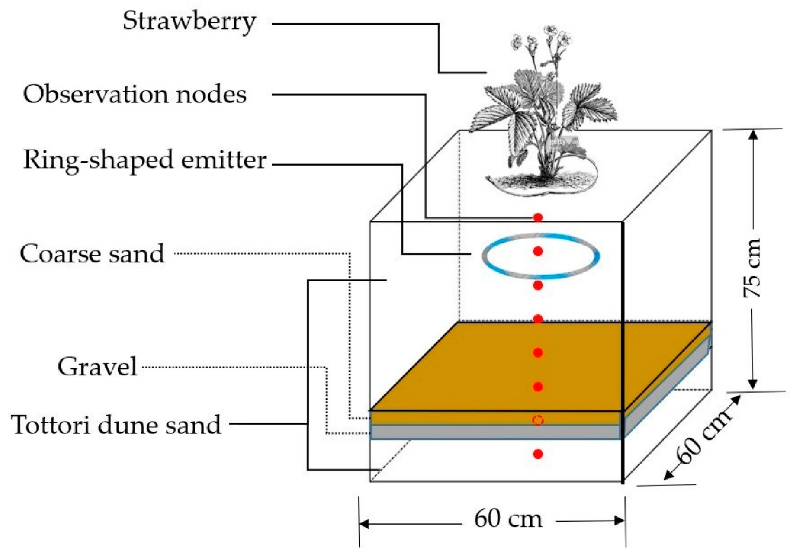
The simulation domain is shown in Figure 3. Since a ring-shaped emitter with five evenly spaced holes was considered, the authors were compelled to use a simulation domain that could fully account for these features. The simulations to analyze the effects of changing the ring-shaped emitter and CB’s installation depths were thus conducted in a fully three-dimensional domain. The size of the domain was 60 × 60 × 75 cm3. The height of the domain was determined according to the vertical root distribution of the strawberry plant. On the other hand, the width and length were set so that the domain’s side boundaries would not affect the water dynamics around the roots in a long-term simulation. The strawberry plant was placed in the center of the domain. The red points in Figure 3 show the positions of observation nodes inserted at a 5 cm interval. Computations were stable for all simulations using this simulation domain.
The domain was assumed to be filled with Tottori dune sand with a CB layer consisting of a 2 cm coarse sand layer and a 3 cm gravel layer placed at a given depth of the Tottori dune sand profile. While the soil hydraulic parameters listed in Table 1 were used for the gravel and coarse sand layers, those inversely estimated by HYDRUS (2D/3D) were used for Tottori dune sand. The ring-shaped emitter was installed in the Tottori dune sand layer above a CB to inject water into the Tottori dune sand profile. The installation depths of the ring-shaped emitter and CB were varied so that their influence on WUE could be evaluated. The ring-shaped emitter was placed at a depth of 10, 20, 30 or 40 cm, while the CB layer was placed at a depth of 45, 50, 55, 60 or 65 cm, resulting in a total number of 20 combinations. The CB depths were determined based on the strawberry’s maximum rooting depth [20]; it is known that the roots may penetrate through the CB layer when it is installed in the root zone [8].
A total volume of 1080 cm3 of water was applied every day during the 28-day simulation. In the inverse estimation of soil hydraulic properties (Section 2.2), the boundary condition at the ring-shaped emitter was a time-variable flux boundary because the water application rate had been previously known from the pot experiment. However, in practice, an irrigation water application rate is normally controlled by a water pressure head at the emitter. Thus, in the investigation of the effect of the emitter and CB’s installation depth on water balance, a time-variable pressure head boundary condition was assigned to the ring-shaped emitter. The original HYDRUS (2D/3D) software package was modified so that the time-variable pressure head boundary condition was switched to a no-flux boundary condition when the cumulative infiltration flux reached or exceeded a given amount of water (i.e., 1080 cm3). Water was applied at the beginning of each day by assigning a zero water pressure head to the ring-shaped emitter. Infiltrated water was then left to redistribute in the soil profile during the rest of the day.
A uniform soil water pressure head of -30 cm was used as the initial condition for the entire soil profile (VWC = 0.084 for Tottori dune sand). This initial condition was determined based on the assumption that the soil profile is reasonably wet when the strawberry plant is at the maturity level shown by the root distribution parameters (Table 2). The potential evaporation rate varies depending on factors such as the growing season and climatic conditions. Stroosnijder [14] reported that the potential evaporation rate is typically between 1 and 6 mm d−1 under semi-arid conditions. For this reason, the potential evaporation rate of 6 mm d−1 was selected and applied to the upper boundary as an atmospheric boundary condition. Hence, combined with the strawberry’s potential transpiration rate of 6 mm d−1 (=720 cm3 d−1) [20], the potential evapotranspiration rate was equal to 12 mm d−1. The atmospheric boundary condition switches from a time-variable flux boundary condition to a constant pressure head boundary condition when the soil water pressure head reaches a predefined minimum pressure head (i.e., hCritA = −80 cm for Totorri dune sand). The hCritA value was determined heuristically based on the agreement between the observed and simulated water contents and the computational stability. No flux was assumed through the lateral sides of the domain. The bottom boundary condition was set as free drainage, representing a zero pressure head gradient at the profile bottom (i.e., allowing for gravity flow).
3. Results
3.1. A Laboratory Experiment with a Ring-Shaped Emitter and a CB
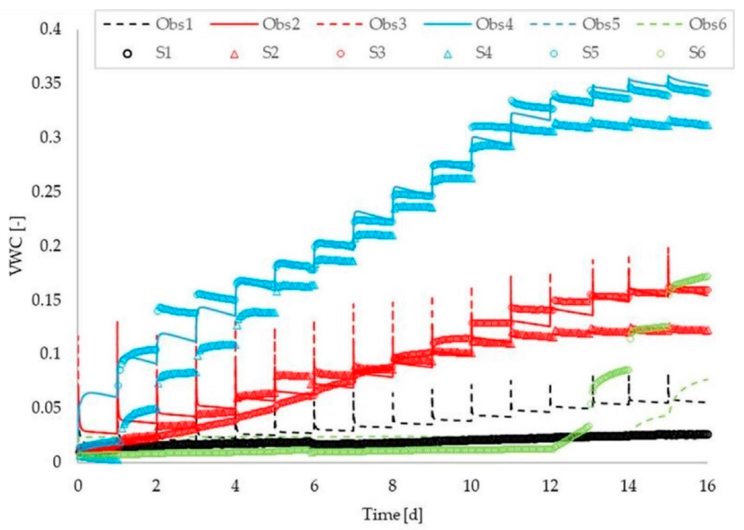
Changes in the soil water content observed by the soil moisture sensors, S1 to S6, are depicted in Figure 4. At S2, S4, and S5, the soil water dynamics pattern can be explained by the following two phases; the soil water content steeply increased immediately after the water application and then leveled off or gradually decreased because of redistribution. The soil water dynamics at S3 followed the same pattern after a quasi-linear increase in VWC before Day 8. No obvious increase in the soil water content was observed at S1 throughout the entire experiment duration. An obvious increase in the soil water content was not observed at S6 until Day 12, indicating that the CB successfully suppressed downward water flow during the first 12 days.
Soil water contents measured on soil samples collected after the experiment are summarized in Table 4. VWCs of the soil samples near the surface (5 cm and 10 cm) slightly varied depending on the horizontal position. The relatively high variability in VWCs near the surface may be attributed to the fact that the effect of evaporation is dominant near the soil surface, making the water dynamics more complicated. However, the horizontal variability in VWCs was small at other depths.
The vertical water distribution shown in Table 4 also confirms that supplied water accumulated upon the CB layer as the samples collected 5 cm above the CB were most wet. This result verified that downward water flow was suppressed at the CB. However, it should also be noted that the CB seems to have been broken during the 16-day experiment, as the VWC 5 cm below the CB is as high as in the layers above the CB. The CB breakage appears to have occurred on Day 12 when the soil water content at S6, located 5 cm below the CB layer, suddenly increased (Figure 4). The CB successfully suppressed downward water flow until Day 12.
3.2. Inverse Estimation of Soil Hydraulic Parameters and Simulation of the Pot Experiment
Table 5 shows the α, n, and l values of Tottori dune sand optimized using the inverse solution of the HYDRUS (2D/3D) software package. These inversely estimated parameter values were then used together with the remaining Durner’s [29] parameters to simulate the soil water dynamics of the pot experiment. Figure 4 shows the changes in the VWC observed at six observation nodes (Obs1-Obs6) in the HYDRUS (2D/3D) simulation along with the VWC observed in the pot experiment (S1–S6). At a depth of 5 cm (S1 and Obs1), the soil water contents predicted by HYDRUS (2D/3D) were in good agreement with observed data, except for predicted temporary increases immediately after water applications. While the observed data at S2–S5 showed that soil water contents varied depending on whether the soil moisture sensor was at the center or near the periphery of the ring-shaped emitter, the HYDRUS (2D/3D) prediction showed no such differences between the observation nodes at the same depth. The CB breakthrough (observed at S6) occurred two days later in the HYDRUS (2D/3D) simulation than in the pot experiment. Besides, the VWCs below the CB were largely underestimated after the breakthrough in the HYDRUS (2D/3D) simulation. Given that the agreement between VWCs measured in the pot experiment and simulated by HYDRUS (2D/3D) was reasonably good at other points, these discrepancies imply that preferential flow (or fingering) might have occurred when water flew through the CB layer.
Overall, the statistical errors between the observed and simulated soil water contents were not significant; the mass balance error [%], the ME [-], the MAE [-], and the RMSE [-] between the observed and predicted values were 0.022%, −0.008, 0.017, and 0.024, respectively.
3.3. Numerical Analysis of the Effect of the Ring-Shaped Emitter and CB Installation Depths
Figure 5 shows the cumulative RWU fluxes expressed as a fraction of AW simulated in the analysis investigating the effect of the installation depth. The ring-shaped emitter and CB were installed at four (10, 20, 30, and 40 cm) and five (45, 50, 55, 60, and 65 cm) different depths, respectively. Two-dimensional soil water distributions under different scenarios can be found in the Supplementary Materials. The RWU value showed a monotonous decrease as an increase in the CB installation depth. While roots were able to extract 41.9% of AW when the emitter and CB were at depths of 10 cm and 45 cm, respectively, they extracted only 14.1% of AW when the emitter and CB were at depths of 10 cm and 65 cm, respectively. This difference shows that the CB installation depth is crucial for the SDI design. When the emitter was at a depth of 10 cm, RWU almost tripled when the CB was moved from a depth of 45 cm to 65 cm. In contrast, RWU increased only by 6.8% by changing the ring-shaped emitter depth from 40 cm to 10 cm with the ring-shaped emitter at a depth of 45 cm.
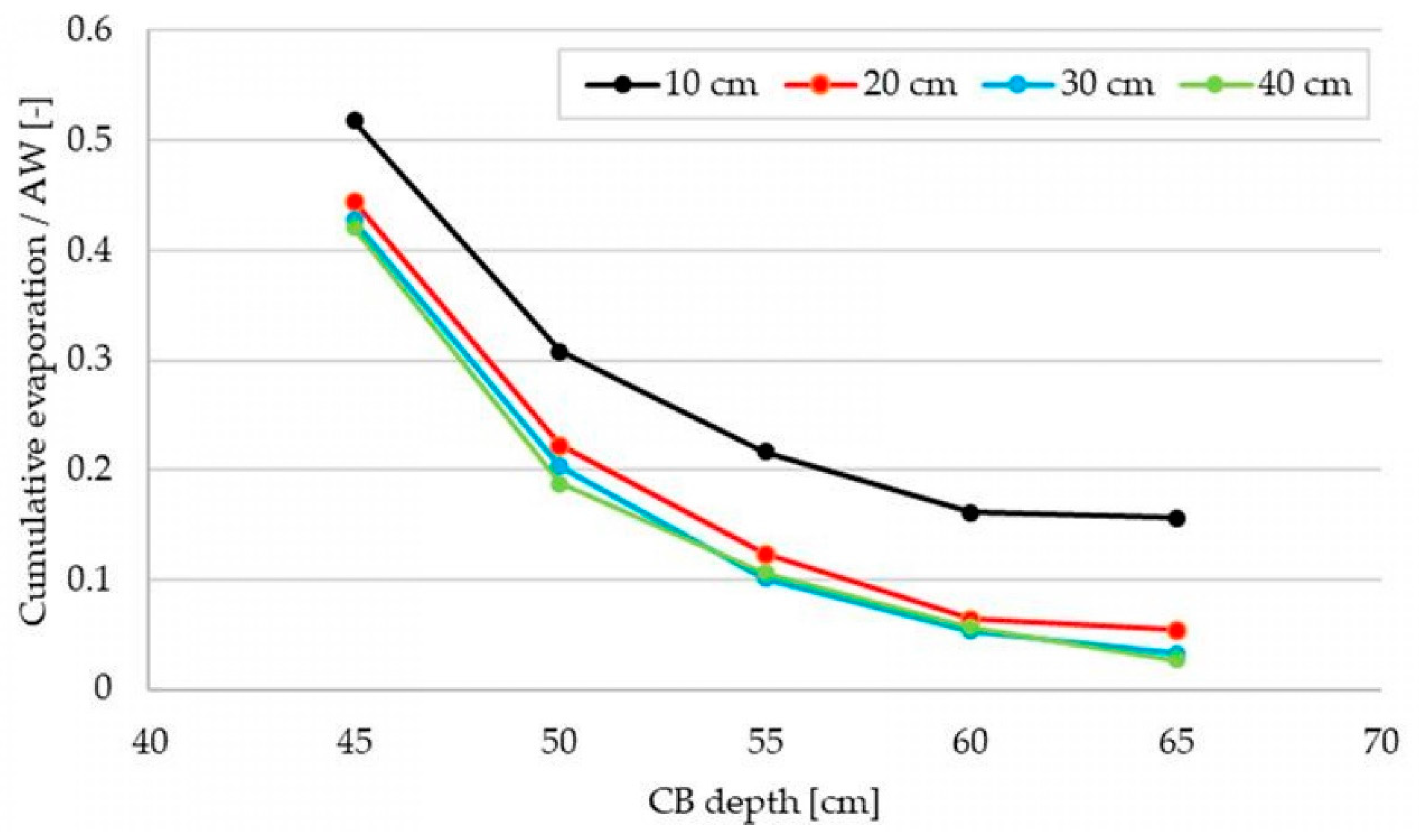
Figure 6 shows the simulated cumulative water loss by evaporation expressed as a fraction of AW when the ring-shaped emitter and CB are at different depths. Similarly, the CB depth had a more significant effect on evaporation than the ring-shaped emitter depth did. With the ring-shaped emitter installed at a depth of 10 cm, 3.3 times more water was lost due to evaporation when the CB was at a depth of 45 cm than at 65 cm. However, the ring-shaped emitter depth strongly influenced the amount of water lost by evaporation as well; with CB at a depth of 45 cm, 16.6% more water was lost by evaporation when the ring-shaped emitter is at a depth of 10 cm than at 20 cm. The effect of the emitter depth was rather small when it was installed deeper than 20 cm. This result exhibits that not only the depth of the CB but also the ring-shaped emitter installation depth is paramount to enhancing WUE.
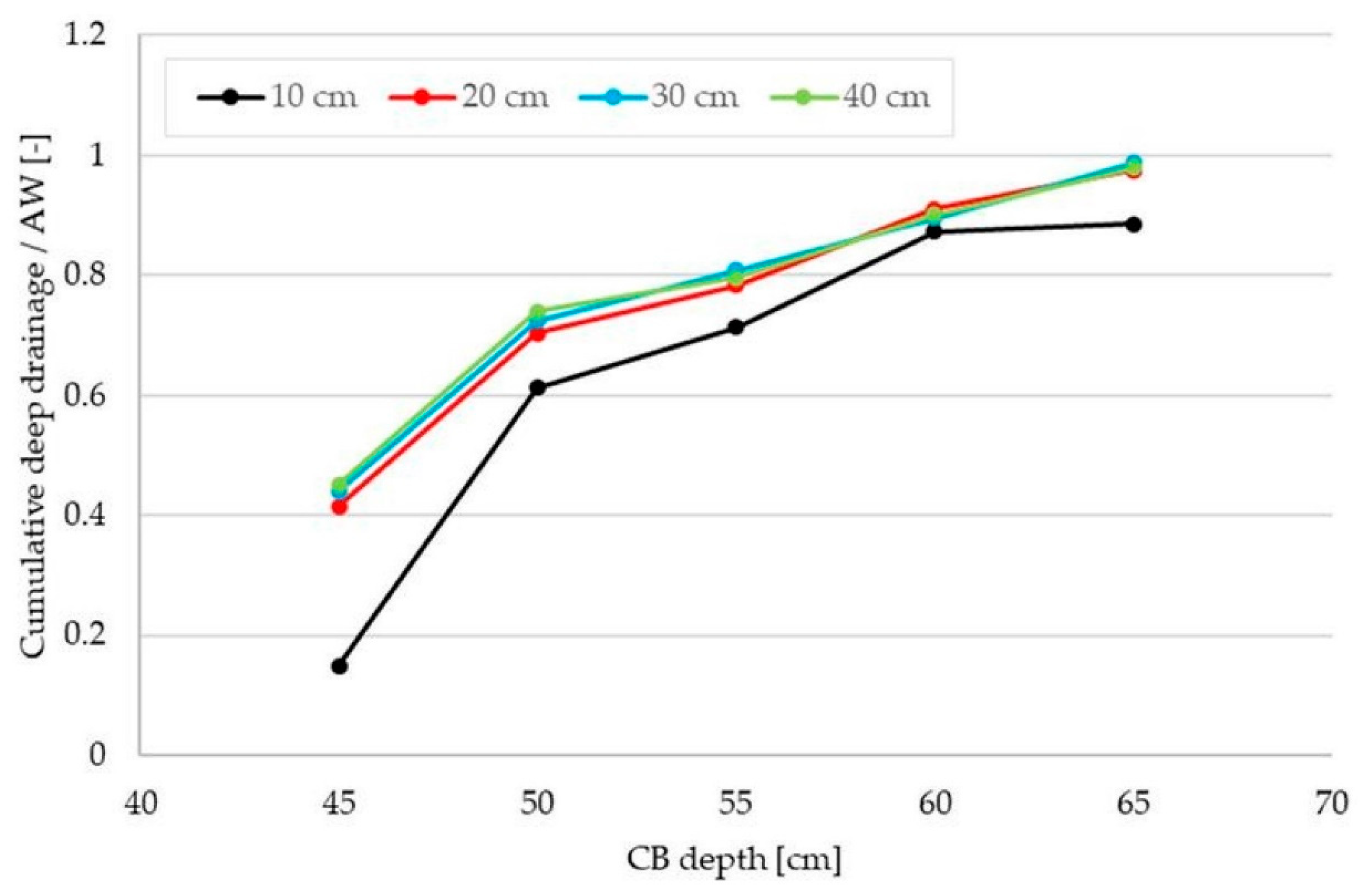
The water loss by deep drainage is also influenced by the installation depth of the ring-shaped emitter and CB (Figure 7). With the CB at a depth of 45 cm, increasing the ring-shaped emitter’s depth from 10 cm to 40 cm resulted in over three times more water loss by deep drainage. When the ring-shaped emitter was at a depth of 10 cm, the CB layer at a depth of 65 cm instead of 45 cm led to approximately six times more water lost due to deep drainage. Deepening the CB led to more water accumulating below the root zone.
4. Discussion
4.1. Water Dynamics in a System with a CB under SDI
The dynamics of the VWC at S3, S4, and S5 in the pot experiment can be explained in the following way: first, the VWC increased when the wetting front reached the soil moisture sensors (Figure 4); then, the VWC gradually decreased or leveled off due to redistribution. Saefuddin et al. [20] studied the VWC fluctuations in the soil profile with the ring-shaped emitter and also reported the surge in the VWC immediately after the water application. However, a decrease in the VWC caused by redistribution was rather steep in the case of Saefuddin and Saito [19]. The gradual decrease or leveling-off observed in this study was likely due to the CB’s effect of suppressing deep percolation. The weak capillary force may explain the limited upward water movement in a relatively coarse material such as Tottori dune sand. Saefuddin et al. [20] also reported that the VWC 5 cm above the ring-shaped emitter in the sand profile did not increase during the 24-hour experiment.
Water accumulation upon the CB layer and its eventual breakage was observed both in the pot experiment and in the HYDRUS (2D/3D) simulation (Figure 4). Between Day 2 and Day 12, most water was retained in the sand layer immediately above the CB. This result verifies that CB’s installation is effective in keeping water in the root zone under SDI, enhancing WUE. The CB breakage was confirmed by an increase in the water content beneath the CB layer on Day 12. The CB breakage occurred after the soil above the CB reached quasi-saturation. Yunasa et al. [11] also reported that water infiltrated into the CB layer when the soil layer immediately above it reached near-saturated conditions. This water accumulation above the CB resulted in the reduction of capillary forces in this upper soil layer and consequent gravitational flow into the coarse sand and gravel layer, causing a partial breakage of CB. After the breakage of CB, an increase in the VWC immediately above the CB became more gradual. This slowdown occurred because accumulated water started infiltrating into the lower layers. Even after the CB breakage, water was retained in the layer immediately above the CB, as the breakage was likely only partial. This result validates the effectiveness of CB under SDI in general.
4.2. The Comparison between the Pot Experiment and the HYDRUS (2D/3D) Simulation
The overall accuracy of the prediction by the HYDRUS (2D/3D) software package was satisfactory. The vertical VWC distribution during the pot experiment was successfully reproduced (Figure 4). The timing of the CB breakage was in good agreement between the pot experiment and the simulation. The obtained error values also confirmed the modeling accuracy. The values were comparable to those reported by the previous studies on the prediction accuracy of HYDRUS (2D/3D) [20,23,24], even though the system in this study was more complex than in the earlier studies. This proves the ability of HYDRUS (2D/3D) to simulate the soil water dynamics in a soil profile with a CB under SDI.
The comparison between the pot experiment results and the HYDRUS (2D/3D) simulation showed two distinct differences. First, while the data obtained in the pot experiment indicated the occurrence of preferential-type non-uniform flow, this process was not considered (and thus could not be reproduced) in the HYDRUS (2D/3D) simulation (Figure 4). The occurrence of non-uniform flow was indicated by the difference in the VWCs obtained at the observation nodes in the same depth. While non-uniform flow might have been induced by the fine-textured textile [34], which covered the ring-shaped emitter, the differences between the observed and simulated VWCs were small (less than 0.033) at the end of the experiment, demonstrating the ability of the ring-shaped emitter to spread water in all directions. The second difference was that the VWC below the CB was underestimated in the HYDRUS (2D/3D) simulation. This may be because the CB breakage occurred only partially, limiting downward water flow through the CB layer. In addition, it is possible that inaccurate soil hydraulic parameters of coarse sand and gravel were used as they were not optimized by HYDRUS (2D/3D). Although the authors attempted to optimize the parameters of the CB materials, this was not successful as the calculations became unstable (due to the parameters of the very coarse CB material). Nevertheless, it should be noted that this discrepancy between the observed and simulated soil water content occurred below the CB. Hence, it does not compromise the effectiveness of the CB or this study’s relevance.
4.3. Effects of the Installation Depths of the Ring-Shaped Emitter and CB on Water Balance
It was shown by the numerical analysis that the depth of the ring-shaped emitter did not influence RWU or water loss as much as the CB depth did. Its effect on RWU was especially limited. However, water losses were influenced by the emitter depth when it was installed shallowly. When the emitter was at a depth of 10 cm, water loss by evaporation largely increased (Figure 6), while water loss by deep drainage decreased (Figure 7). The shallow installation of the ring-shaped emitter led to the high soil water content near the surface, which is known to increase the actual evaporation rate [15]. Thus, there seems to be a trade-off regarding the way water is lost depending on the emitter installation depth. In practice, the installation depth should also be determined in light of other factors such as the installation cost and irrigation water quality.
In contrast, the CB depth substantially influences both RWU and water loss by evaporation and deep drainage. The shallow installation of the CB at a depth of 40 cm led to the most active strawberry RWU, which indicates that water stress on the strawberry’s root was alleviated. This is because strawberry plants actively extract water near the soil surface (5 cm below the surface) [20]. Therefore, the installation depth of the CB needs to be determined considering the type of plants, as root characteristics largely affect RWU and water loss by deep drainage [35]. Field cultivation experiments with various kinds of plants will provide further guidance on the ideal CB depth.
As shown in Figure 6, the shallow installation of the CB also caused higher water loss by evaporation because the soil near the surface was kept wet. Ityel et al. [5] also reported that the shallower the CB, the more water was retained near the surface. As the soil water content near the surface enhances the evaporation rate [15], evaporation is likely to intensify in the presence of a shallow CB. This phenomenon was also reported by Miyake et al. [8], who reported that evapotranspiration intensified when an effective CB layer was present. The numerical analysis in this study revealed that the evaporation rate, as well as the VWC just above the CB, are affected by its installation depth and that the evaporation rate depends not only on the presence of the CB but also on its installation depth. This result indicates that the CB should be installed deep if the goal is to reduce evaporation.
Water loss by deep drainage was also affected by the CB depth. While the shallow CB led to an increase in evaporation, the deep CB caused higher water losses by deep drainage due to the CB breakage. When the CB layer is installed deep below the root zone, less water can be retained in the root zone. More water then flows downwards without being absorbed by the root, resulting in water accumulation upon the CB layer and hence its eventual breakage. Vertical water movement depends on the soil types under SDI [20]. The effect of soil types on the preferable CB installation depth will further aid the development of the designs of SDI with a CB.
Overall, these findings strongly indicate that the agricultural water demand in arid regions can be significantly reduced without harming crop production or additional costs by improving on-farm SDI designs. Such improvements will greatly alleviate pressures on scarce water resources, as 70% of freshwater resources are used globally for agricultural production [1]. Given that this study has validated the effectiveness of a CB under SDI, its application under various conditions (soil types, plant types, etc.) should be explored further. Such exploration will contribute to disseminating water-efficient agricultural practices and tackling water scarcity in semi-arid and arid regions.
5. Conclusions
Enhancing agricultural WUE is critical in both arid and semi-arid regions. The installation of a CB has been suggested as a promising engineering approach to reduce water loss by deep drainage. This is the first study that evaluated the effectiveness of a CB installation in a soil profile under SDI to the best of our knowledge. The pot experiment results showed that a CB could aid in retaining water in the upper soil layer under SDI, even after its eventual breakage. The inverse estimation of soil hydraulic parameters and statistical analysis proved that HYDRUS (2D/3D) [22] could predict soil water dynamics in a relatively complex soil profile with a ring-shaped emitter and a CB. The numerical analysis indicated that CB’s shallow installation increased water retention near the soil surface and the strawberry’s RWU. However, it also increased water loss by evaporation [15]. In contrast, water loss by deep drainage increased when a CB was installed deep. The effect of the ring-shaped emitter’s depth on the water balance was relatively limited. Overall, this study’s findings agree well with past studies on the ring-shaped emitter [17,19,20] and CB [5,6,8,9]. Further testing and application of the proposed SDI systems under various conditions (e.g., crop types, climatic conditions) will aid in ensuring water and food security.
Supplementary Materials
The following are available online at https://www.mdpi.com/article/10.3390/w13091300/s1. Figure S1. Two-dimensional soil water distribution profiles with a CB at a depth of 45 cm and 65 cm and with the ring-shaped emitter at a depth of 10 cm and 40 cm, respectively.
Author Contributions
Conceptualization, H.S., K.N., and R.S.; methodology, K.N.; software, J.Š.; validation, K.N.; writing—original draft preparation, K.N.; writing—review and editing, H.S. and J.Š.; funding acquisition, H.S. All authors have read and agreed to the published version of the manuscript.
Funding
This study was financially supported by JSPS Grant-in-aid Scientific Research Program (17H03885 and 20H03097) and by the Joint Research Program of Arid Land Research Center, Tottori University.
Institutional Review Board Statement
Not applicable.
Informed Consent Statement
Not applicable.
Data Availability Statement
The data that support the findings of this study are available from the corresponding author upon reasonable request.
Conflicts of Interest
The authors declare no conflict of interest.
References
- Steduto, P.; Faurès, J.-M.; Hoogeveen, J.; Winpenny, J.; Burke, J. Coping with Water Scarcity: An Action Framework for Agricultural and Food Security; FAO WATER REPORTS 38; Food and Agricultural Organization of the United Nations: Rome, Italy, 2012; pp. 11–13, ISSN 1020-1203. [Google Scholar]
- Grasham, C.F.; Korzenevica, M.; Charles, K.J. On considering climate resilience in urban water security: A review of the vulnerability of the urban poor in sub-Saharan Africa. WIREs Water 2019, 6, e1344. [Google Scholar] [CrossRef] [Green Version]
- Niang, I.; Ruppel, O.C.; Abdrabo, M.A.; Essel, A.; Lennard, C.; Padgham, J.; Urquhart, P. Climate Change 2014: Impacts Adaptation, and Vulnerability. Part B: Regional Aspects. Contribution of Working Group 2 to the Fifth Assessment Report of the Intergovernmental Panel on Climate Change; Cambridge University Press: Cambridge, UK, 2014; pp. 1199–1265. [Google Scholar] [CrossRef] [Green Version]
- Sousa, P.M.; Blamey, R.C.; Reason, C.J.C.; Ramos, A.M.; Trigo, R.M. The ‘Day Zero’ Cape Town drought and the poleward migration of moisture corridors. Environ. Res. Lett. 2018, 13, 124025–124035. [Google Scholar] [CrossRef] [Green Version]
- Ityel, E.; Lazarovitch, N.; Silberbush, M.; Ben-Gal, A. An artificial capillary barrier to improve root zone conditions for horticultural crops: Physical effects on water content. Irrig. Sci. 2010, 29, 171–180. [Google Scholar] [CrossRef]
- Ityel, E.; Lazarovitch, N.; Silberbush, M.; Ben-Gal, A. An artificial capillary barrier to improve root zone conditions for horticultural crops: Response of pepper, lettuce, melon, and tomato. Agric. Water Manag. 2012, 30, 293–301. [Google Scholar] [CrossRef]
- Ityel, E.; Lazarovitch, N.; Silberbush, M.; Ben-Gal, A. An artificial capillary barrier to improve root zone conditions for horticultural crops: Response of pepper plants to matric head and irrigation water salinity. Irrig. Sci. 2012, 105, 13–20. [Google Scholar] [CrossRef]
- Miyake, M.; Otsuka, M.; Fujimaki, H.; Inoue, M.; Saito, H. Evaluation of an Artificial Capillary Barrier to Control Infiltration and Capillary Rise at Root Zone Areas. J. Arid Land Stud. 2015, 25, 117–120. [Google Scholar] [CrossRef]
- Wongkaew, A.; Saito, H.; Fujimaki, H.; Šimůnek, J. Numerical analysis of soil water dynamics in a soil column with an artificial capillary barrier growing leaf vegetables. Soil Use Manag. 2018, 34, 206–215. [Google Scholar] [CrossRef]
- Mohammed, S.A.; Rashid, A.; Said, S.A.; Anvar, R.K.; Hamed, A. Use of Soil-Structured Capillary Barrier can Mitigate the Impact of Saline Irrigation Water on Marigold Grown Under Field Condition. J. Agri. Mar. Sci. 2020, 25, 9–19. [Google Scholar] [CrossRef]
- Yunasa, G.H.; Kassim, A.; Umar, M.; Talib, Z.A.; Abdulfatah, A.Y. Laboratory investigation of suction distribution in a modified capillary barrier system. IOP Conf. Ser. Earth Environ. Sci. 2020, 476, 012047. [Google Scholar] [CrossRef]
- Morris, C.E.; Stormont, J.C. Evaluation of numerical simulations of capillary barrier field tests. Geotech. Geol. Eng. 1998, 16, 201–213. [Google Scholar] [CrossRef]
- Fala, O.; Molson, J.; Aubertin, M.; Bussière, B. Numerical Modelling of Flow and Capillary Barrier Effects in Unsaturated Waste Rock Piles. Mine Water Environ. 2005, 24, 172–185. [Google Scholar] [CrossRef]
- Stroosnijder, L. Soil evaporation: Test of a practical approach under semi-arid conditions. Neth. J. Agri. Sci. 1987, 35, 417–426. [Google Scholar] [CrossRef]
- Bonachela, S.; Orgaz, F.; Villalobos, F.J.; Fereres, E. Soil evaporation from drip-irrigated olive orchards. Irrig. Sci. 2001, 20, 65–71. [Google Scholar] [CrossRef]
- Martinez, J.; Reca, J. Water use efficiency of surface drip irrigation versus an alternative subsurface drip irrigation method. Irrig. Drain. Eng. 2014, 140, 04014030. [Google Scholar] [CrossRef]
- Friedman, S.P.; Gamliel, A. Wetting Patterns and Relative Water-Uptake Rates from a Ring-Shaped Water Source. Soil Sci. Soc. Am. J. 2019, 83, 48–57. [Google Scholar] [CrossRef]
- O’Brien, D.M.; Rogers, D.H.; Lamm, F.R.; Clark, G.A. An Economic Comparison of Subsurface Drip and Center Pivot Sprinkler Irrigation Systems. Appl. Eng. Agric. 1998, 14, 391–398. [Google Scholar] [CrossRef]
- Saefuddin, R.; Saito, H. Performance of a ring-shaped emitter for subsurface irrigation in bell pepper (Capsicum annum L.) cultivation. Paddy Water Environ. 2019, 17, 101–107. [Google Scholar] [CrossRef]
- Saefuddin, R.; Saito, H.; Šimůnek, J. Experimental and numerical evaluation of a ring-shaped emitter for subsurface irrigation. Agric. Water Manag. 2019, 211, 111–122. [Google Scholar] [CrossRef]
- Sumarsono, J.; Setiawan, B.I.; Subrata, I.D.M.; Saptomo, S.K. Ring-typed emitter subsurface irrigation performances in dryland farmings. Int. J. Civ. Eng. Technol. 2018, 9, 797–806. [Google Scholar]
- Šimůnek, J.; van Genchten, M.T.; Sejna, M. Recent Developments and Applications of the HYDRUS. Computer Software Packages. Vadose Zone J. 2016, 6, 1–25. [Google Scholar] [CrossRef] [Green Version]
- Skaggs, T.H.; Trout, T.J.; Šimůnek, J.; Shouse, P.J. Comparison of HYDRUS-2D Simulations of Drip Irrigation with Experimental Observations. Irrig. Drain. Eng. 2004, 130, 304–310. [Google Scholar] [CrossRef]
- Kandelous, M.M.; Šimůnek, J. Comparison of numerical, analytical, and empirical models to estimate wetting patterns for surface and subsurface drip irrigation. Irrig. Sci. 2010, 97, 1070–1076. [Google Scholar] [CrossRef] [Green Version]
- Šimůnek, J.; van Genuchten, M.T.; Šejna, M. The HYDRUS Software Package for Simulating Two- and Three-Dimensional Movement of Water, Heat, and Multiple Solutes in Variably-Saturated Media, Technical Manual, 3rd ed.; PC Progress: Prague, Czech Republic, 2018; pp. 103–106. [Google Scholar]
- Provenzano, G. Using HYDRUS-2D simulation model to evaluate wetted soil volume in subsurface drip irrigation system. Irrig. Drain. Eng. 2007, 133, 342–349. [Google Scholar] [CrossRef]
- El-Nesr, M.N.; Alazba, A.A.; Šimůnek, J. HYDRUS simulations of the effects of dual-drip subsurface irrigation and a physical barrier on water movement and solute transport in soils. Irrig. Sci. 2014, 32, 111–125. [Google Scholar] [CrossRef] [Green Version]
- Brunetti, G.; Šimůnek, J.; Piro, P. A comprehensive analysis of the variably saturated hydraulic behavior of a green roof in a Mediterranean climate. Vadose Zone J. 2016, 5, 1–17. [Google Scholar] [CrossRef] [Green Version]
- Durner, W. Hydraulic conductivity estimation for soils with heterogeneous pore structure. Water Resour. Res. 1994, 30, 211–223. [Google Scholar] [CrossRef]
- van Genuchten, M.T. A closed-form equation for predicting the hydraulic conductivity of unsaturated soils. Soil Sci. Soc. Am. J. 1980, 44, 892–898. [Google Scholar] [CrossRef] [Green Version]
- Šimůnek, J.; van Genuchten, M.T.; Sejna, M. Development and applications of the HYDRUS and STANMOD software packages and related codes. Vadose Zone J. 2008, 7, 587–600. [Google Scholar] [CrossRef] [Green Version]
- Vrugt, J.A.; van Wijk, M.T.; Hopmans, J.W.; Šimůnek, J. One-, two-, and three-dimensional root water uptake functions for transient modeling. Water Resour. Res. 2001, 37, 2457–2470. [Google Scholar] [CrossRef] [Green Version]
- Feddes, R.A.; Kowalik, P.J.; Zaradny, H. Simulation of Field Water Use and Crop Yield; John Wiley & Sons: New York, NY, USA, 1978; ISBN 9789022006764. [Google Scholar]
- Jury, W.A.; Horton, R. Soil Physics, 6th ed.; John Wiley & Sons: New York, NY, USA, 2004; pp. 139–146. ISBN 978-0-471-05965-3. [Google Scholar]
- Kandelous, M.M.; Kamai, T.; Vrugt, J.A.; Šimůnek, J.; Hanson, B.; Hopmans, J.W. Evaluation of subsurface drip irrigation design and management parameters for alfalfa. Agric. Water Manag. 2012, 109, 81–93. [Google Scholar] [CrossRef]
Figure 1.
Configuration of the ring-shaped emitter (adapted from Saefuddin et al. [20]).
Figure 1.
Configuration of the ring-shaped emitter (adapted from Saefuddin et al. [20]).

Figure 2.
(a) A vertical cross-section and (b) top view of the setup of the pot experiment. Red points S1–S6 show the positions of the soil moisture sensors. Points P1–P4 show the horizontal positions where soil samples were collected at the end of the experiment.
Figure 2.
(a) A vertical cross-section and (b) top view of the setup of the pot experiment. Red points S1–S6 show the positions of the soil moisture sensors. Points P1–P4 show the horizontal positions where soil samples were collected at the end of the experiment.

Figure 3.
The simulation domain of the HYDRUS (2D/3D). The depths of the ring-shaped emitter and CB were varied.
Figure 3.
The simulation domain of the HYDRUS (2D/3D). The depths of the ring-shaped emitter and CB were varied.

Figure 4.
Soil water dynamics in the pot experiment. S1–S6 indicate soil water contents measured using the soil moisture sensors in the pot experiment, while Obs1–Obs6 show corresponding soil water contents simulated by HYDRUS (2D/3D) using the optimized soil hydraulic parameters.
Figure 4.
Soil water dynamics in the pot experiment. S1–S6 indicate soil water contents measured using the soil moisture sensors in the pot experiment, while Obs1–Obs6 show corresponding soil water contents simulated by HYDRUS (2D/3D) using the optimized soil hydraulic parameters.

Figure 5.
Cumulative RWU expressed as a fraction of AW during the 28-day simulations when the ring-shaped emitter and CB are at different depths. The results for different ring-shaped emitter depths (10, 20, 30, and 40 cm) are shown using lines of different colors.
Figure 5.
Cumulative RWU expressed as a fraction of AW during the 28-day simulations when the ring-shaped emitter and CB are at different depths. The results for different ring-shaped emitter depths (10, 20, 30, and 40 cm) are shown using lines of different colors.

Figure 6.
Cumulative evaporation expressed as a fraction of AW during the 28-day simulations when the ring-shaped emitter and CB are at different depths. The results for different ring-shaped emitter depths (10, 20, 30, and 40 cm) are shown using lines of different colors.
Figure 6.
Cumulative evaporation expressed as a fraction of AW during the 28-day simulations when the ring-shaped emitter and CB are at different depths. The results for different ring-shaped emitter depths (10, 20, 30, and 40 cm) are shown using lines of different colors.

Figure 7.
Cumulative deep drainage expressed as a fraction of AW during the 28-day simulations when the ring-Scheme 10, 20, 30, and 40 cm) are shown using lines of different colors.
Figure 7.
Cumulative deep drainage expressed as a fraction of AW during the 28-day simulations when the ring-Scheme 10, 20, 30, and 40 cm) are shown using lines of different colors.


Table 1.
Initial estimates of the soil hydraulic parameters of Tottori Dune sand, coarse sand, and gravel for the Durner [29] model.
Table 1.
Initial estimates of the soil hydraulic parameters of Tottori Dune sand, coarse sand, and gravel for the Durner [29] model.
| Materials | θr [-] | θs [-] | α1 [cm−1] | n [-] | Ks [cm/min] | w1 [-] | w2 [-] | α2 [cm−1] | n2 [-] | l [-] |
|---|---|---|---|---|---|---|---|---|---|---|
| Tottori Dune sand | 0.006 | 0.384 | 0.030 | 6.675 | 2.15 | 1.0 | 0 | 0 | 1.5 | 0.5 |
| Coarse sand | 0.004 | 0.371 | 0.133 | 20.8 | 4.97 | 0.99 | 0.01 | 0.25 | 1.5 | 0.5 |
| Gravel | 0.005 | 0.274 | 0.204 | 15.5 | 13.8 | 0.99 | 0.01 | 0.25 | 1.5 | 0.5 |
| Vrugt et al. (2001) Parameter Description | Variable | Value |
|---|---|---|
| Maximum rooting radius [cm] | Xm | 20 |
| Radius of maximum intensity [cm] | x* | 0 |
| Maximum rooting radius [cm] | Ym | 20 |
| Radius of maximum intensity [cm] | y* | 0 |
| Maximum rooting depth [cm] | Zm | 30.5 |
| Depth with maximum rooting density [cm] | z* | 5 |
| Non-symmetry coefficient [-] | Px, Py, Pz | 1, 1, 1 |
| Surface area associated with transpiration [cm2] | - | 1200 |
Table 3.
The Feddes et al. [33] parameters for strawberries (modified from those presented in Saefuddin et al. [20] to improve the computational stability).
| Feddes et al. [33] Parameters | Value |
|---|---|
| h1 [cm] | −5 |
| h2 [cm] | −10 |
| h3 [cm] | −40 |
| h4 [cm] | −45 |
Table 4.
VWC distribution measured at the end of the pot experiment.
| Measurement Depth | VWC | Ave. | SD. | ||||
|---|---|---|---|---|---|---|---|
| P1 | P2 | P3 | P4 | Center | |||
| 5 cm | 0.071 | 0.031 | 0.061 | 0.023 | 0.014 | 0.040 | 0.022 |
| 10 cm | 0.085 | 0.071 | 0.087 | 0.049 | 0.053 | 0.069 | 0.016 |
| 15 m | 0.136 | 0.150 | 0.177 | 0.178 | 0.145 | 0.157 | 0.017 |
| 20 cm | 0.213 | 0.224 | 0.238 | 0.255 | 0.244 | 0.235 | 0.015 |
| 25 cm | 0.294 | 0.331 | 0.338 | 0.331 | 0.326 | 0.324 | 0.016 |
| Coarse sand layer | 0.084 | 0.083 | 0.085 | 0.082 | 0.089 | 0.085 | 0.003 |
| Gravel layer | 0.032 | 0.041 | 0.039 | 0.030 | 0.036 | 0.036 | 0.004 |
| 40 cm | 0.212 | 0.199 | 0.194 | 0.163 | 0.218 | 0.197 | 0.019 |
Table 5.
The initial estimates and optimized parameter values of Tottori dune sand.
| α [cm−1] | n [-] | l [-] | |
|---|---|---|---|
| Initial estimates | 0.03 | 6.665 | 0.5 |
| Optimized values | 0.0502 | 4.748 | 0.00227 |
Publisher’s Note: MDPI stays neutral with regard to jurisdictional claims in published maps and institutional affiliations. |
© 2021 by the authors. Licensee MDPI, Basel, Switzerland. This article is an open access article distributed under the terms and conditions of the Creative Commons Attribution (CC BY) license (https://creativecommons.org/licenses/by/4.0/).
Share and Cite
MDPI and ACS Style
Noguchi, K.; Saito, H.; Saefuddin, R.; Šimůnek, J. Evaluation of Subsurface Drip Irrigation Designs in a Soil Profile with a Capillary Barrier. Water 2021, 13, 1300. https://doi.org/10.3390/w13091300
AMA Style
Noguchi K, Saito H, Saefuddin R, Šimůnek J. Evaluation of Subsurface Drip Irrigation Designs in a Soil Profile with a Capillary Barrier. Water. 2021; 13(9):1300. https://doi.org/10.3390/w13091300
Chicago/Turabian StyleNoguchi, Koichi, Hirotaka Saito, Reskiana Saefuddin, and Jiří Šimůnek. 2021. "Evaluation of Subsurface Drip Irrigation Designs in a Soil Profile with a Capillary Barrier" Water 13, no. 9: 1300. https://doi.org/10.3390/w13091300
Note that from the first issue of 2016, this journal uses article numbers instead of page numbers. See further details here.