
Hunting for Information in Streamflow Signatures to Improve Modelled Drainage


1
Department of Hydrology, Geological Survey of Denmark and Greenland, DK-1350 Copenhagen, Denmark
2
Department of Water Resources, Ramboll Denmark, DK-2300 Copenhagen, Denmark
*
Author to whom correspondence should be addressed.
Water 2022, 14(1), 110; https://doi.org/10.3390/w14010110
Submission received: 9 November 2021
/
Revised: 10 December 2021
/
Accepted: 29 December 2021
/
Published: 5 January 2022
(This article belongs to the Section Water, Agriculture and Aquaculture)
Abstract
:About half of the Danish agricultural land is drained artificially. Those drains, mostly in the form of tile drains, have a significant effect on the hydrological cycle. Consequently, the drainage system must also be represented in hydrological models that are used to simulate, for example, the transport and retention of chemicals. However, representation of drainage in large-scale hydrological models is challenging due to scale issues, lacking data on the distribution of drain infrastructure, and lacking drain flow observations. This calls for more indirect methods to inform such models. Here, we investigate the hypothesis that drain flow leaves a signal in streamflow signatures, as it represents a distinct streamflow generation process. Streamflow signatures are indices characterizing hydrological behaviour based on the hydrograph. Using machine learning regressors, we show that there is a correlation between signatures of simulated streamflow and simulated drain fraction. Based on these insights, signatures relevant to drain flow are incorporated in hydrological model calibration. A distributed coupled groundwater–surface water model of the Norsminde catchment, Denmark (145 km2) is set up. Calibration scenarios are defined with different objective functions; either using conventional stream flow metrics only, or a combination with hydrological signatures. We then evaluate the results from the different scenarios in terms of how well the models reproduce observed drain flow and spatial drainage patterns. Overall, the simulation of drain in the models is satisfactory. However, it remains challenging to find a direct link between signatures and an improvement in representation of drainage. This is likely attributable to model structural issues and lacking flexibility in model parameterization.
1. Introduction
Around the world, agricultural land is commonly artificially drained to prevent flooding and increase crop yield. With its temperate climate and gentle topography, Denmark is no exception to this. About 66% of Denmark’s land area is used for agriculture, of which about half is assumed to be artificially drained, mainly by tile drains [1]. Drains have a profound effect on the entire hydrological cycle and in particular on groundwater flow and related transport of chemicals, particles and nutrients [2,3,4,5,6]. Tile drain provides a short-cut from the field to surface water bodies, bypassing transport in the deep aquifers. This is crucial to nitrate transport, as nitrate can be reduced only under anaerobic conditions, which primarily are found in the deeper groundwater systems [7,8,9]. Consequently, insight into the amount and dynamics of drain flow is essential to understand and quantify transport of nitrate or other substances.
Despite the importance of tile drains for the transport of chemicals in agricultural watersheds, there remain significant unresolved challenges in representing drainage in hydrological models beyond the field scale. (1) The actual location of subsurface drain systems is often unknown (e.g., [10]). Where information exists, it typically is limited to small patches, but even in these cases knowledge on the drain network is commonly unprecise. At large scales, there only exist estimates of tile drain locations in Denmark based on proxy data [1,11]. (2) Similarly, there is a lack of drain flow observations, which only exist for few field-scale catchments. Generally, drain flow shows high spatio-temporal variability. (3) Likewise, due to the coarse spatial resolution of large-scale hydrological models, tile drain processes cannot be represented explicitly in the model (for a discussion see [8,12]). The resulting simplified representation of drain processes in large-scale models lead to an aggregation of hydrological processes: typically, drain is described implicitly, and also accounts for underrepresentation of the surface water network in the model. Furthermore, the distribution of drain flow is, amongst other factors, controlled by small-scale variations in topography, often below model resolution. For regional or large-scale models, no relevant observations of drain flow are available. The resolution of such models—currently, the national water resource model of Denmark (DK-model, [13,14]), has a horizontal resolution of 500 m or 25 ha per model cell—is at or above typical catchment areas of drain flow observations reported in literature (e.g., [15,16]).
Due to these challenges, a more indirect way to regionalize and evaluate the representation of drain flow in regional- and large-scale hydrological models is needed. Here we suggest the use of hydrological signatures, which are indices characterizing hydrological behaviour. Most commonly, hydrological signatures are scalar values derived from time series of streamflow. Common examples are flow quantiles, base flow index, runoff coefficient, or the slope of the flow duration curve. There exist a large number of signatures, see e.g., [17,18] for extensive, yet not exhaustive, overviews because of the almost limitless possibility to design new signatures [19]. Some signatures may only contain information relating to specific parts of a catchment response, and many will contain similar or redundant information. Hence, before analysis, signatures relevant to the specific purpose have to be selected carefully [19].
Hydrological signatures are used to characterize different runoff processes such as groundwater contributions, overland flow or snow melt (see [20] for a review). Field studies have shown correlation between signature values and catchment states such as soil moisture, even though such correlations are complex and challenging to establish [21]. Furthermore, signature values can be related to physical catchment properties and climatic variables [22], and they are commonly used to characterize different aspects of catchment responses. The information contained in signatures is exploited to classify catchments, regionalize hydrological models and predictions, and improve predictions in ungauged basins [18,23,24,25]. Signatures are also used to evaluate hydrological model performance in a more specific way compared to conventional performance indicators, such as Nash–Sutcliffe efficiency (NSE) or Kling–Gupta efficiency (KGE). This allows for better detection of deficiencies in the representation of different hydrological processes in the models [26,27]. The ability of models to reproduce hydrological signatures has been linked to better process representation due to increased model complexity or more advanced input data (e.g., [28,29,30] and a review [20]). Eventually, streamflow signatures were considered in the calibration of hydrological models [31,32,33], often motivated by the additional information contained in signatures over conventional criteria of goodness of fit. This can be beneficial in data-scarce settings, where a signature-domain calibration can be easier to perform than a conventional time-domain calibration, for example because properties such as recession curves can be extracted even from inaccurate time series [34].
Drain flow is a distinct runoff-generating process. In heavily drained agricultural areas, it contributes to a significant share of total stream discharge [5,35,36]. Furthermore, drain flow has specific characteristics, such as quick responses to precipitation events and interactions with the groundwater table dynamics [8,16]. Hence, drain flow will have an effect on the hydrograph [37], even in streams that aggregate contributions from a variety of runoff-generating processes. So far, correlations between hydrological signatures in streams and artificial drainage have only been exploited to a limited extent to inform hydrological models [38].
The objective of this work is to evaluate the potential of using hydrological signatures to improve the representation of drain in regional-scale distributed hydrological models. To do so, we
- Test the hypothesis that hydrological signatures hold information on the contribution of drain flow to total streamflow.
- Test the degree to which model calibration can be guided and drain flow simulation improved by including selected hydrological signatures in the objective functions.
2. Data and Methods
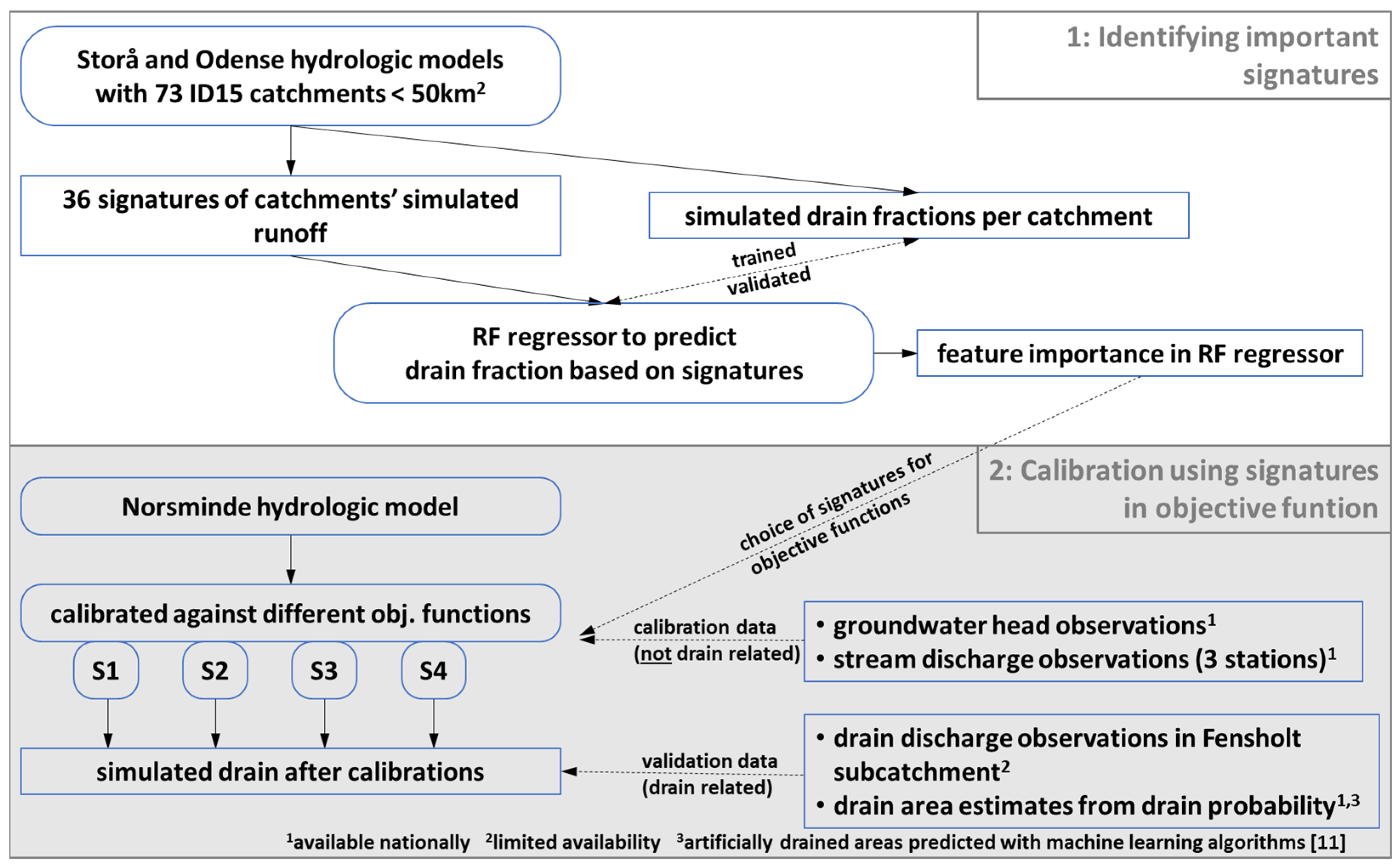
Ideally, the analysis surrounding the first objective would be carried out based on observed streamflow as well as observed drain flow, but this is impossible due to the limited amount of drain flow observations. The analysis was therefore based on simulations from integrated, distributed hydrological models (Section 2.2; upper part of Figure 1). The relationship between simulated streamflow signatures and simulated drain flow was examined for two Danish catchments, the Storå catchment in western Jutland and the Odense catchment on the island of Funen (Figure 2). The catchments are 1124 km2 and 1004 km2, respectively, and were chosen to represent the diversity of the Danish landscape: the Storå catchment exhibits gentle topographical variation and is dominated by naturally well drained sandy soils, while the Odense catchment has a slightly more varied topography and is dominated by clayey soils. In both cases, data were extracted for various topographical sub-catchments providing a large dataset for the further analyses.
Based on the knowledge gained, in the second step it was analysed how simulation of drain flow in regional-scale models can be informed by including selected hydrological signatures in model calibration. We employed alternative objective functions with a mixture of conventional performance criteria and hydrograph signatures (Section 2.3; bottom part of Figure 1). For a robust assessment, the calibration was carried out in a third independent catchment, the Norsminde catchment in eastern Jutland (Figure 3) with a size of about 145 km2. This catchment was also chosen as it is the best studied Danish catchment with respect to drain flow [8,12,39], and includes several stations with drain flow measurements.
2.1. Hydrological Modelling
All three hydrological models used in the present study were set up as transient, distributed, coupled surface water–groundwater models in the hydrological modelling framework MIKE SHE [40,41]. The model system couples 3D subsurface flow, 2D overland flow and 1D routing of surface water in streams. The unsaturated zone is conceptualized as a two-layer water balance model, the 2-Layer method of MIKE SHE [41] (p. 27).
The hydrological model conceptualization and data for the three models are based on the National Water Resource Model of Denmark (DK-model) developed at the Geological Survey of Denmark and Greenland (GEUS) [13,14,42]. The description of the subsurface is based on a hydrogeological model interpreted in a 100 m grid covering all of Denmark. The numerical models have the same 100 m horizontal resolution, and a varying number of layers of different thickness depicted by the site-specific hydrogeology, with unit-based parameterization. The top layer has a constant thickness of 2 m and is parameterized based on the Danish soil map [43]. Climate data were provided by the Danish Meteorological Institute (DMI) as gridded, daily data with precipitation in 10 km and temperature as well as evapotranspiration in 20 km resolution [44,45]. Precipitation data were corrected as described in [46].
The two larger models, Storå and Odense were originally developed in a project evaluating an increase in the resolution of the DK-model from 500 m to 100 m, focussing on an improved representation of the uppermost groundwater table [47]. The calibration approach for these models resembles that used as the baseline for the Norsminde model (scenario S1, Section 2.3.4). For more details on the models used in step 1 to establish a link between hydrological signatures and simulated drain, the reader is referred to the provided reference.
The model used in step 2, Norsminde, builds on previous modelling work concerning drain flow and nitrate transport for the same catchment by [39]. A detailed description of the model follows in Section 2.3.
2.2. Machine Learning Regressors to Predict Drain Fraction
Initial tests revealed correlations between different simulated streamflow signatures and the simulated drain fraction: For example, the Pearson correlation coefficients between each of the six most important signatures and the respective simulated drain fractions range from 0.51 to 0.75. However, we were not successful using linear regression models to predict drain fraction based on signatures.
Hence, to establish whether there is a correlation between signatures and the prevalence of artificial drain within a catchment, we performed machine learning aided regressions. This work was performed using the implementation of Random Forest (RF) regressors in the python package scikit-learn. RF regressors typically allow exploitation of more complex correlations between explanatory variables better than linear regression models (being observed in a similar context for example by [48]).
Drain fraction is defined as the ratio between temporally averaged drain flow and averaged total streamflow for a certain catchment area. That is, the drain fraction is a value between 0 and 1 indicating the share of the total runoff in a catchment that originates from drain flow. Drain flow is taken from the spatial output of MIKE SHE aggregated for each ID15 catchment, and compared to the simulated streamflow at the outlet of each respective catchment outlet. For more details on how MIKE SHE simulates drain flow, please refer to Section 2.3.1 below.
2.2.1. Simulated Discharge Used in Machine Learning Regression
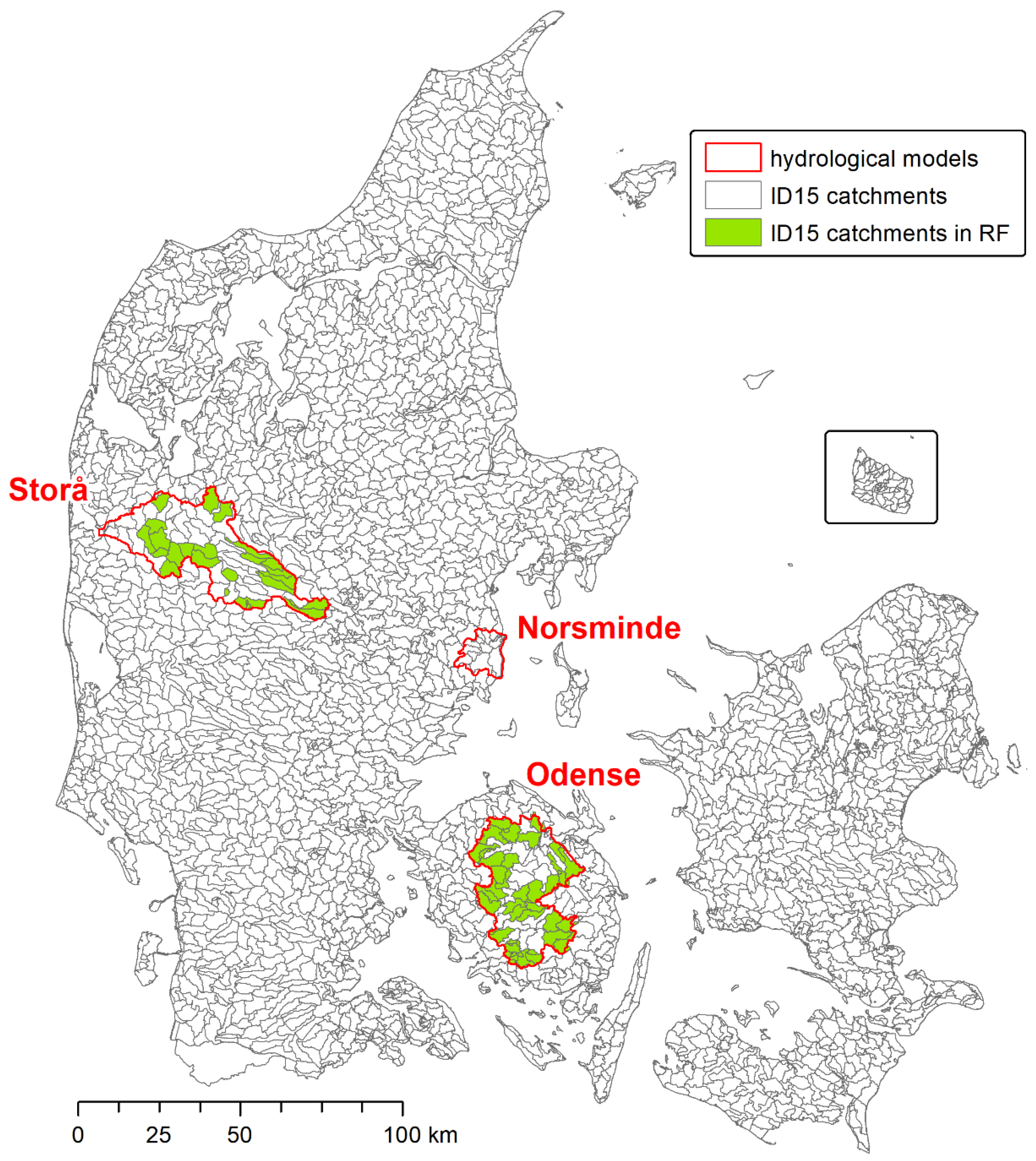
Data for the machine learning regression were established by hydrological modelling, where stream and drain discharge were extracted from topographical sub-catchments. The entirety of Denmark was delineated into hydrological catchments with an average size of 15 km2, referred to as ID15 catchments (outlined grey in Figure 2). For the analysis, all individual headwater ID15 catchments from both models were selected and supplemented by downstream ID15 catchments for which the aggregated catchment area was below 50 km2. This resulted in a dataset of 73 catchments (48 from Odense and 25 from Storå, green in Figure 2). An upper threshold for the catchment area was applied as the signal from drain flow is diluted for increasing catchment size: a performance decrease in the regression models was observed when increasing the threshold. This effect has been shown before, though for significantly larger catchment sizes [37].
The entire analysis described in the following was based on the simulated hydrographs with daily timesteps for the 9 full years from 2000 to 2008. For this, simulated discharge in the streams at the outlet of each catchment was considered, i.e., catchments varying from approximately 15 to 50 km2.
2.2.2. Hydrological Signatures
A set of 36 hydrological signatures was calculated for the 73 time series of daily discharge at the catchment outlets, shown in Table 1. The signatures were calculated in python, partly assisted by the SPOTPY package [49]. The set of signatures was chosen based on the expected impacts of drain flow on hydrographs, for example baseflow characteristics, variability of flows, or seasonal variations, as drains in Denmark are predominantly active in winter. Furthermore, the timing and size of the first response at the onset of the drain season in fall, where the shallow groundwater table has just raised above drain level, are difficult to match in hydrological models [50], and “first peak” signatures were therefore included.

Table 1.
List of hydrological signatures used as explanatory variables in machine learning regressors.
Table 1.
List of hydrological signatures used as explanatory variables in machine learning regressors.
| Signature | Unit | Explanation | |
|---|---|---|---|
| BFI5 | Baseflow index, 5-day period | - | For entire time series, and separate for each season |
| BFI5 w/s | BFI5 winter/summer ratio | - | Summer: Jun, Jul, Aug. Winter: Jan, Feb, Mar |
| BFI20 | Baseflow index, 20-day period | - | |
| SFDC | Slope of the middle third of the flow duration curve | - | |
| rcoeff | Runoff coefficient | - | Precipitation taken from model forcing |
| CV | Coefficient of variation | - | For entire time series, and separate for each season |
| CV w/s | Coefficient of variation winter/summer | - | |
| RBFI | Richards–Baker–Flashiness index | - | [51] |
| skew | skewness: mean (q)/median (q) | - | |
| mriser | Mean change in q while hydrograph is rising | mm/d | |
| mfallr | Mean change in q while hydrograph is falling | mm/d | |
| qm | Mean specific runoff | mm | For entire time series, and separate for each season |
| qm w/s | Mean specific runoff winter/summer ratio | - | |
| f2ms | first peak after Aug 1st > 2 × mean (q summer) | doy | As indication for start of flow from tile drains |
| fp3ms | first peak after Aug 1st > 3 × mean (q summer) | doy | As indication for start of flow from tile drains |
| fp2m | first peak after Aug 1st > 2 × median (q) | doy | As indication for start of flow from tile drains |
| fp3m | first peak after Aug 1st > 3 × median (q) | doy | As indication for start of flow from tile drains |
| Qq99 | 0.99 flow quantile | mm/d | |
| Qq95 | 0.95 flow quantile | mm/d | |
| Qq90 | 0.90 flow quantile | mm/d | |
| Qq10 | 0.10 flow quantile | mm/d | |
| Qq5 | 0.05 flow quantile | mm/d | |
| Qq1 | 0.01 flow quantile | mm/d | |
| hQv | High flow variability | - | Mean of annual maximum q/median q |
| lQv | Low flow variability | - | Mean of annual minimum q/median q |
| lfD | Low flow duration | d/y | Average number of days per year where q < 0.5 × mean (q) |
| lfED | Low flow event duration | d | Average length of events of q < 0.5 × mean (q) |
| lfEF | Low flow event frequency | y−1 | Occurrences of q < 0.5 × mean (q) |
| hfD | High flow duration | d/y | Average number of days per year where q > 3 × median (q) |
| hfED | High flow event duration | d | Average length of events of q > 3 × median (q) |
| hfEF | High flow event frequency | y−1 | Occurrences of q > 3 × median (q) |
| minq7d | Mean minimum discharge measured over 7 consecutive days | mm/d | |
| minq30d | Mean minimum discharge measured over 30 consecutive days | mm/d | |
| maxq7d | Mean maximum discharge measured over 7 consecutive days | mm/d | |
| maxq30d | Mean maximum discharge measured over 30 consecutive days | mm/d | |
| catcharea | Catchment area | km2 | (only physical catchment characteristic used in analysis) |
2.3. Norsminde Hydrological Model
To test how the inclusion of hydrograph signatures affect calibration of a hydrological model, the Norsminde Fjord catchment (Figure 3) was set up. This catchment is situated in eastern Jutland, Denmark. The geology is dominated by clay, with marine sediments in the deeper layers. In the south of the model area, those deeper layers are incised by a buried valley with complex glacial deposits. The top 10 to 50 m are comprised of glacial deposits, dominated by clay [52]. In total, the model area encompasses 154 km2, of which 145 km2 are land surface, with the remainder being sea. Generally, the topographic variation is gentle, with the western part of the catchment being hillier reaching up to elevations of about 100 m above sea level. In its centre, the town of Odder is located, whereas the rest of the catchment is dominated by agriculture. The built-up area accounts for about 14% of the catchment’s land surface area, and intensive agriculture for 65%. In combination with the prevalence of clayey soils, this means that a large fraction of the agricultural area is drained by tile drains.
The saturated zone of the hydrological model was conceptualized in 10 computational layers, based on a nationwide hydrogeological interpretation (Fælles offentlig hydrologisk model FOHM [53]) established from detailed hydrological modelling as part of the national groundwater mapping program. The parametrization of the subsurface is unit-based, i.e., each hydrogeological unit is assigned homogenous model parameters for hydraulic conductivity etc. Daily precipitation data were available from Fillerup station in the catchment from 27 October 2012 to 4 September 2017. Outside this period, and for temperature and evapotranspiration forcing, national gridded data as described in Section 2.1 were used. For further details on the general model setup, please refer to the references provided in Section 2.
2.3.1. Hydrological Model—Drain Setup
Artificial drainage structures, such as ditches and drain pipe networks, cannot be represented explicitly for typical model grid resolutions in large-scale hydrological models. Furthermore, as the exact location of artificial drains are unknown, drainage is accounted for in the model setup by including drain in all model cells. In this way, simulated drain flow encompasses both the actual artificial drain through drain pipes, and also any potential small-scale network of ditches and streams and the effects of microtopography [54] that cannot be represented due to the coarse scale of the model. The implementation of drains in the model thus implies that all areas where drainage is needed, i.e., high groundwater tables occur, are in fact drained, which reflects the agricultural land use management in Denmark.
In MIKE SHE, simulated drain is controlled by a drain depth and time constant [41] (p. 202). Drain depth is defined relative to the surface level, resulting in a drainage level Zdr. In any given model cell, drainage is only active if the simulated groundwater level h exceeds the drainage level. In this case, the drain time constant Cdr controls how quickly groundwater is removed as drain flow qdr:
In our case, the generated drain flow is directly routed to the nearest stream within each ID15 catchment.
The drain time constant and depth were distributed across the model domain according to seven land use classes (shown in Figure 3), based on an aggregation of the 36-class landuse map BASEMAP [55] as shown in Table 2. The drain time constants in Table 2 were used as a starting point in the calibration, and were treated as a single free parameter, maintaining their initial ratios throughout parameter changes in the calibration. Drain depths were not calibrated.
Areas close to rivers are generally discharge areas and may discharge either directly to the streams through overland flow, the stream bed, or via drainage. As the true drain distribution in these areas is unknown, the amount of generated drain flow in model cells adjacent to a model stream cannot be reliably discriminated from the amount of river baseflow generated. For this reason, simulated drain flow in river link cells [56] (p. 69) was excluded from the analysis.
2.3.2. Hydrological Model—Calibration Data
For the evaluation of the performance of the hydrological model, different data sources were used:
Firstly, daily discharge observations are available from three discharge stations (270002, 270003, and 270035 in Figure 3) that are part of the Danish National Monitoring and Assessment Programme for the Aquatic and Terrestrial Environment (NOVANA) [57]. Furthermore, discharge observations from the outlet of the Fensholt sub-catchment were available. Those data originate from previous modelling and monitoring work in the region (the iDRÆN project, Aarhus University, https://idraen.dk/, accessed on 28 December 2021).
Secondly, groundwater head observations were extracted from GEUS’ Denmark-wide well database Jupiter (https://eng.geus.dk/products-services-facilities/data-and-maps/national-well-database-jupiter/, accessed on 28 December 2021). For the period 2007 to 2017, a total of almost 18,000 head observations are available within the Norsminde catchment, distributed across 316 intakes (marked in Figure 3). In some wells continuous time series of observed groundwater heads exist, whereas other wells only provide a single observation.
These two datasets were used in model calibration, as described in Section 2.3.4. Following model calibration, the models’ ability to represent drainage was evaluated based on the drain-related datasets described in the following section.
2.3.3. Hydrological Model—Drain Validation Data
Generally, it is challenging to evaluate the representation of artificial drainage in our models due to mentioned issues of scale and data scarcity. However, a Denmark-wide map of the probability for artificial drainage exists [11], which is used to evaluate the spatial distribution of simulated drainage. This map shows the probability for artificial drainage on agricultural land estimated using machine learning regressors. It is based on point information on artificial drain conditions at 745 points across Denmark, with a set of geological, topographical, climate and land use information as explanatory variables. As suggested by the creators of the map, a probability threshold of 50% to distinguish drained and undrained areas was used, resulting in a binary map discriminating drained and undrained areas. According to this dataset, about 88% of the non-urban, non-forested area in the Norsminde catchment is likely being drained artificially. In a similar manner, binary maps of drained and undrained areas were created based on the model results. Here, the distinction was made based on a threshold for the average simulated drain flow per cell. The threshold value was adjusted to ensure that the total drained area in the Norsminde catchment as predicted by the model results matches the total area predicted by the drain probability map. This analysis was limited to the extent of the drain probability map, which excludes urban and forested areas. Furthermore, as mentioned above, simulated drain cannot reliably be extracted from river link cells in the model and those areas were also excluded from the analysis. In the model evaluation, the areas predicted by the models to be actively draining were compared to the drain areas predicted by the drain probability map.
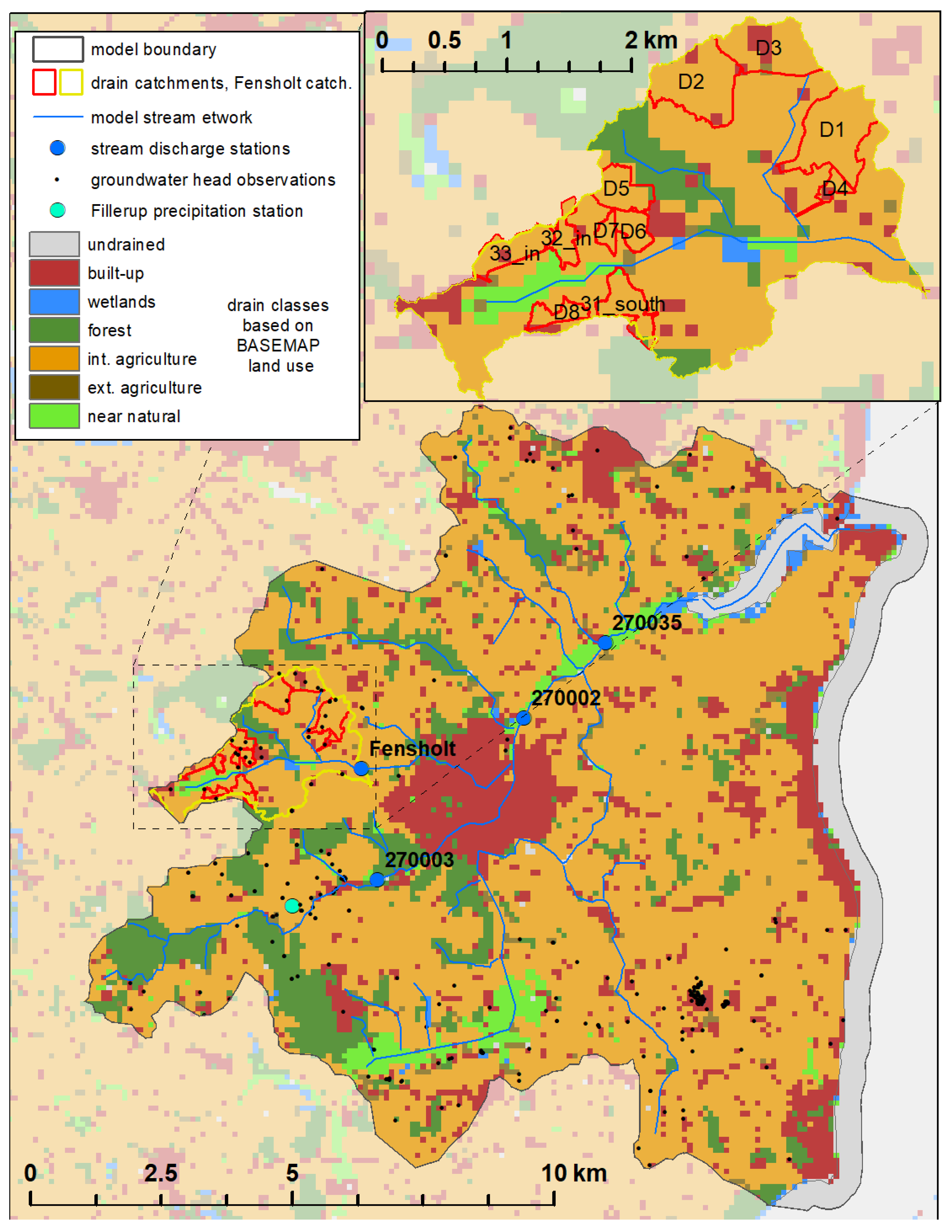
Another option for evaluating the models’ performance in representing drain is comparing time series of simulated drain flow to observations of drain flow. Within the Fensholt sub-catchment daily observations of flow from tile drains exists from 11 stations. The observations were collected in the iDRÆN and TReNDS (http://trends.nitrat.dk/, accessed on 28 December 2021) projects [58]. The estimated catchments of the 11 drain stations are outlined in Figure 3. Data availability for eight of the stations (D1 to D8) was roughly six years, from autumn 2012 to the end of 2017, with some gaps. From the remaining three stations (31_south, 32_in, 33_in), data is only available since October 2016 or April 2017.
For a direct comparison of observed and simulated daily drain flow, only stations D1 to D8 with longer data availability were used. The validation period was chosen as 7 November 2012 to 8 August 2017. The observations from all eleven stations, however, were used to obtain an observation-based estimate of drain flow from the entire Fensholt sub-catchment. Area specific drain flow was calculated from the observed drain catchments, which was assumed to be representative for all drained agricultural areas within Fensholt. For the extrapolation, only the agricultural area of the sub-catchment was considered (4.6 km2 of the total of 6.1 km2), and the percentage of drained agricultural area was taken from the drain probability map, showing that 83% of the agricultural land within is artificially drained. Hence, the total artificially drained area in the Fensholt sub-catchment was estimated to 3.8 km2. On average across the validation period, 34% of this area was covered by drain flow observations.
Based on these drain flow data and streamflow observations from the outlet of the sub-catchment, drain fractions were calculated, and compared to the respective simulated values. Due to inherent uncertainties, drain fractions were not calculated based on daily data, but aggregated monthly.
2.3.4. Hydrological Model—Calibration Setup
The hydrological model was calibrated with the PEST software package for parameter estimation [59], using a Gauss–Marquardt–Levenberg local search algorithm. The calibration period was 1 January 2007 to 31 December 2017, with a 10 year-warmup period for each run. Based on the observation data (Section 2.3.2), objective functions were formulated as weighted aggregation of performance metrics for stream discharge, including the selected hydrological signatures, and for groundwater heads. Discharge performance was evaluated using the KGE [60]. Out of the four discharge stations, only the three from the national dataset were used in the calibration, as only such stations would be available for national-scale model setups. Furthermore, the fourth station at the outlet of the Fensholt sub-catchment only has data since late 2012; this station was used in the calculation of drain flow from the Fensholt sub-catchment.
The groundwater head observations consist of well data. Each well can contain either a single observation of the water level, or a time series of water levels, from one or more screens at different depths. Where more than one observation (spatially and/or temporally) was available in a model grid, the residuals between observed and simulated heads were averaged. The mean errors per model grid then were weighted based on the number of observations—with a weight of 1 for cells with one observation, a weight of 2 for cells with two to nine observations, a weight of 3 for cells with ten to 99 observations, and a weight of 5 for cells with 100 or more observations. The final objective function for groundwater heads was formulated using the Continuous Ranked Probability Score (CRPS), as described by [61]. The CRPS-based approach was chosen because conventionally used squared-error-based objective functions are particularly sensitive to large residuals. In the context of large or regional-scale hydrological models with large datasets of not purely scientific origin (such as our dataset of groundwater heads), large residuals are often a result of observational errors or model structural errors, but not necessarily informative in the parameter estimation process.
The calibration only employing KGE for streamflow (and CRPS for groundwater heads) is referred to as scenario S1, with a relative weight of 2/3 on KGE and 1/3 on groundwater head performance. Three further calibration scenarios were carried out that included hydrological signatures in the objective function. Signature performance was included in the objective function as the residuals between the signature value of the simulated and the observed hydrograph, minimizing the discrepancy between simulated and observed value. In those cases, the relative weights between the objective function groups were 1/3 on KGE, 1/3 on signatures and 1/3 on groundwater head performance. S2 included one signature, S3 two signatures, while six signatures were included in S4. Table 3 gives an overview over the calibration scenarios.
3. Results
3.1. RF Regressors Predicting Drain Fraction
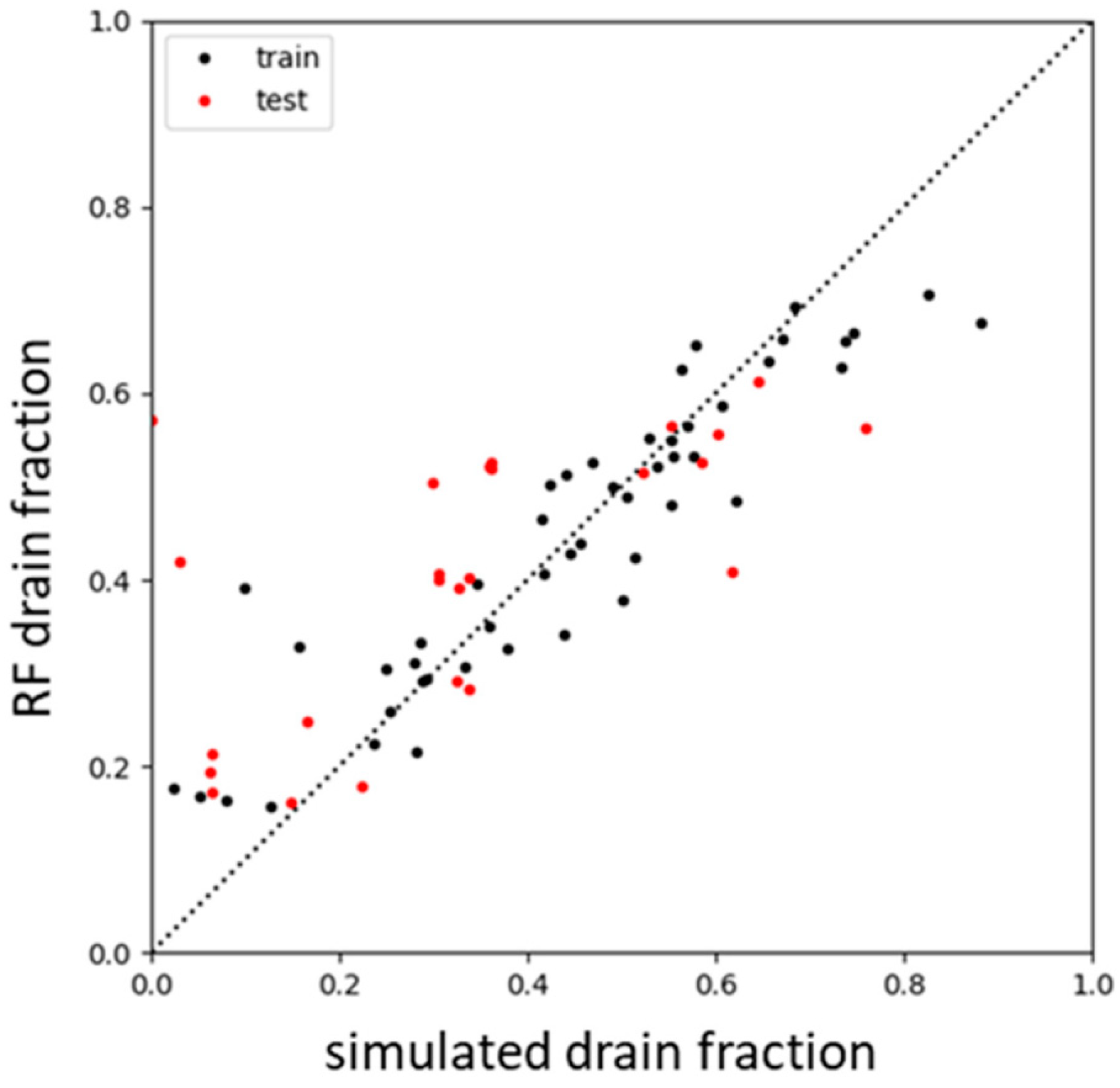
As described in Section 2.2, we performed machine learning aided regressions, evaluating the correlation between streamflow signatures and drain fraction. The RF regressor was trained on two thirds of the 73 sub-catchments of the Storå and Odense Å models, Figure 2, while the remaining sub-catchments were used for test. The results are shown in Figure 4, where all 36 hydrograph signatures were used as explanatory variables and the simulated drain fraction as target variable. Based on the model simulations, it was found that the drain fraction could be well described by the hydrograph signatures, with a mean absolute error on the predicted drain fraction of 0.126 for the test dataset. In other words, there is a correlation between streamflow signatures and the fraction of streamflow that originates from artificial drain (drain fraction) within a catchment—a precondition for the following calibration experiments, where we incorporated streamflow signatures in the objective function of the model calibration to improve its representation of artificial drain.
RF regressors allow exploration of which explanatory variables—hydrological signatures in our case—are most important for the predictive capability of the regressor model. A common implementation for determining the so-called feature importance is by randomly perturbing each explanatory variable one at a time, thereby effectively removing the information it holds. Calculating the decrease in performance of the regressor model as one explanatory variable is perturbed provides a measure of the importance of that variable. Using this approach, the high flow event duration (hfED) showed to be most important, with a decrease in the goodness-of-fit between RF predicted and simulated drain fraction of about 27%. The second most important signature was the skewness (7%). These two were followed by several signatures with performance decreases by around 2%. From these, the coefficient of variation (CV), the ratio between specific runoff during winter and summer (qm w/s), the low flow event duration (lfED), and the slope of the flow duration curve (SFDC) were selected, while the rest were left out based on considerations of redundancy: for example, the specific runoff in spring, summer and fall showed importance almost as high as the ratio qm w/s; however, those are somewhat correlated and considered redundant information.
The six mentioned hydrological signatures were then used in the hydrological model calibration experiments with the Norsminde model, hypothesizing that a better fit to those signatures results also in a better representation of different runoff-generating processes in the model, including artificial drain.
3.2. Evaluation of the Hydrological Model Calibration Scenarios
3.2.1. Evaluation against Calibration Data
Four different calibration scenarios, Table 3, were compared, where S1 represents a calibration only including the KGE as conventional performance criterion for discharge. S2 to S4 additionally incorporate different hydrological signatures in the objective function.
Table 4 provides an overview of the resulting model performance. Groundwater head performance is given as mean error (ME) and mean absolute error (MAE) across all intakes. Streamflow metrics are given as mean across the three discharge stations. The metrics that are part of the objective function in each scenario are in bold font. Both the fit of the model to the observed groundwater heads and the general streamflow (KGE and water balance) are largely unaffected by including signatures in the objective function. Including signatures in the objective function results—as is to be expected—in models representing the observed signatures better.
3.2.2. Evaluation against Drain-Related Validation Data
The models’ performance in representing artificial drain flow was evaluated in three ways: (1) at field level by comparing observed and simulated daily time series of drain flow from the eight drain catchments, (2) aggregated drain flow as monthly mean values for the Fensholt sub-catchment, and (3) the spatial distribution of areas with drainage.
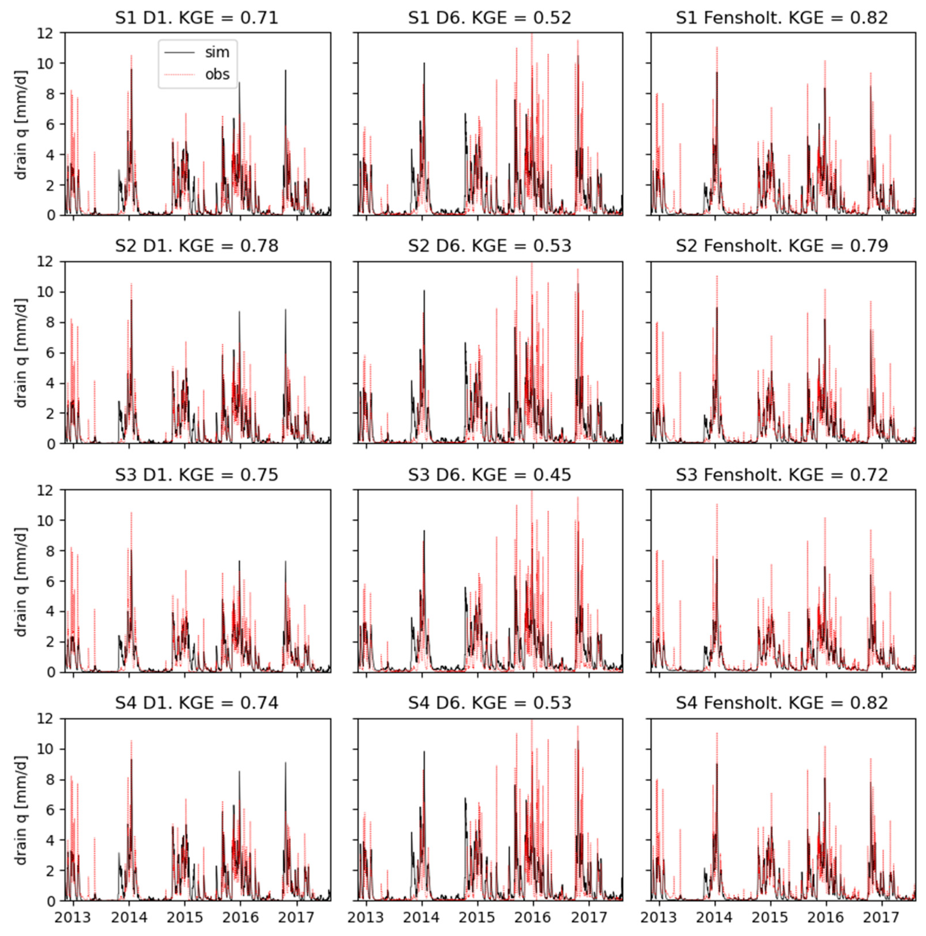
Comparison of simulated and observed drain flow at field scale is presented in Figure 5, where the first two columns show daily time series of simulated and observed drain flow for two selected drain catchments. The last column shows simulated drain flow across the entire Fensholt sub-catchment, where the observed time series is based on extrapolation of the drained area covered by observations as described in Section 2.3.3. Each row presents the results of one of the calibration scenarios.
The overall model results are encouraging, with a mean KGE across the eight individual drain catchments between 0.36 and 0.52 (first row of Table 5) and a KGE between 0.72 and 0.82 for drain flow from the entire Fensholt sub-catchment. However, as seen in Figure 5, the effect of including the hydrographs signatures in the objective function differs for the individual drain catchments/fields. For drain catchment D1 drain flow is described well by all models, even the base case S1 without signatures. In this case the inclusion of hydrograph signatures does improve the model fit, especially when just one signature is included. The same cannot be said about drain catchment D6. In general, model performance is slightly worse here. For example, the model simulates early peaks in autumn 2013 and 2014 that cannot be seen in the observations, and the model fails to match the peak response in the winter of 2015/2016. The first issue likely indicates a model structural error such as the interpretation of the subsurface geology, resulting in a simulated groundwater table that rises too fast at the onset of the draining season in autumn. The second issue also could suggest that the observation data are noisy. While parameter adjustment through calibration is not sufficient to compensate for model structural errors, the different model calibrations do impact the overall drainage generated in D6. Nevertheless, the performance of the alternative calibrations is contradicting the hypothesis that including signatures improves drain representation. Evaluating across the entire Fensholt sub-catchment the effect of including the hydrograph signatures varies, with S1 and S4 being equally good, while the results are worse especially in the case where two signatures are included.
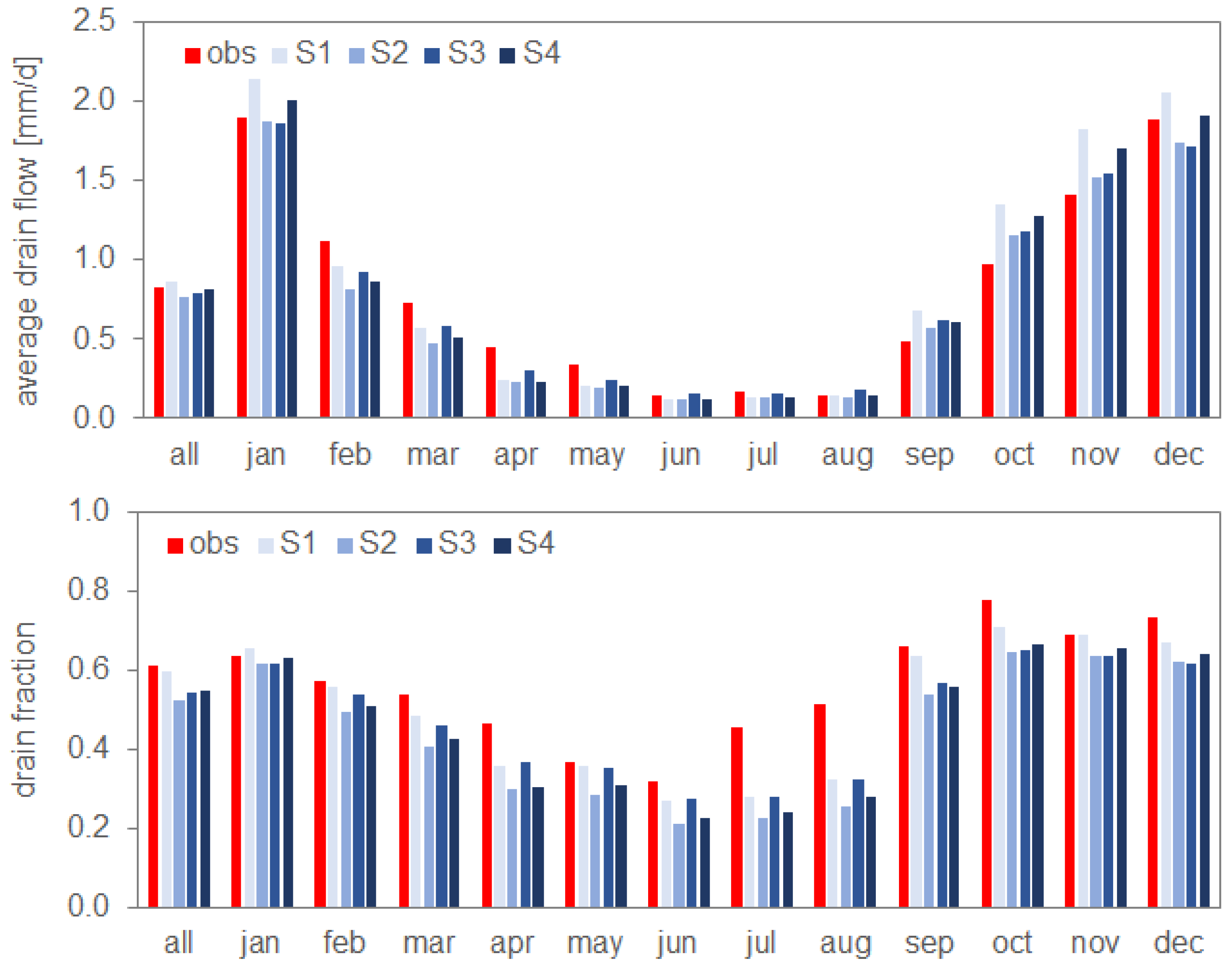
The model evaluation for aggregated monthly values across the Fensholt sub-catchment is presented in Figure 6, where the top plot shows the average drain flow, and the bottom the resulting drain fraction. There is generally a very good agreement between observed and simulated monthly drain flow for the Fensholt sub-catchment. However, the base case without signatures overestimates drain flow through most of autumn and winter, which is less pronounced in the scenarios including signatures. S4 results in drain flow estimates that are generally larger than the two other scenarios which include signatures (S2 and S3).
Only small variations are observed in the calculated drain fractions among the four model scenarios. The monthly observed drain fractions are captured very well by the models except for a tendency to underestimation in summer and autumn. As simulated drain flows for those months are matched or slightly overestimated, this indicates that the models overestimate the total runoff during those months. It is notable that the average drain flow across the entire period from the Fensholt sub-catchment of 0.87 mm/d accounts for a large part of net precipitation of 1.06 mm/d (precipitation of 2.37 mm/d, actual evapotranspiration 1.31 mm/d; values for S1).
Based on the average monthly drain flow and drain fractions the inclusion of the hydrograph signatures appears to improve the drain flow simulation in absolute numbers, while the calculated drain fractions are almost unaffected. During summer, drain and streamflow is low; calculating the drain fraction thus is prone to high uncertainties, as small differences in absolute flow values can result in large deviations in the relative values of drain fraction.
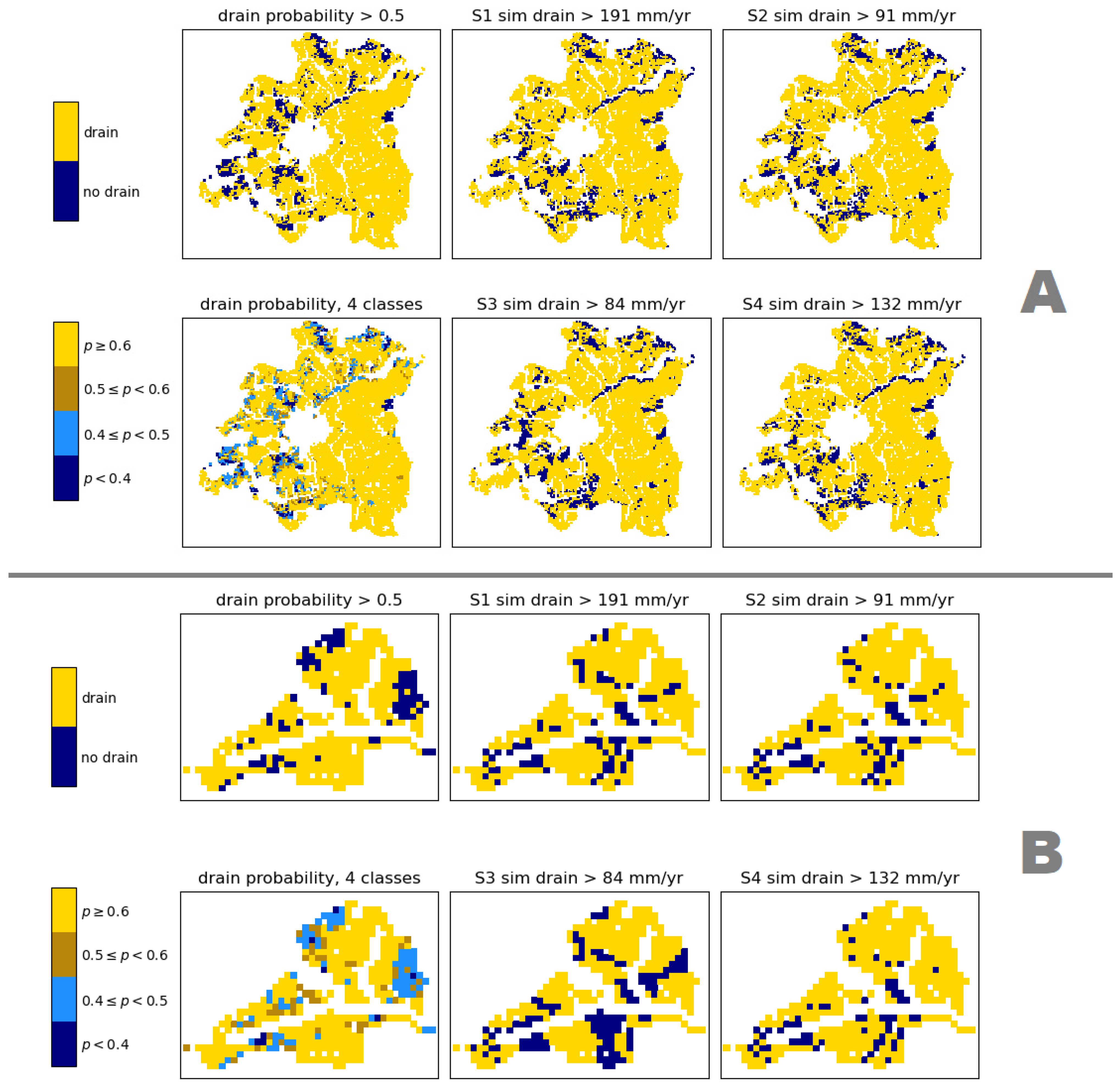
The spatial evaluation of drain occurrence was made by dividing the catchment into zones that are likely artificially drained and not drained. This division was based on the amount of simulated drain flow, where all model grids draining above a certain threshold were assumed to be drained, while no active drainage was assumed for the rest. The threshold of simulated drain flow was chosen so that the resulting total drained area matches the total drained area in the validation data, the artificial drain probability map by [11]. This threshold differs from scenario to scenario: For S1, the threshold is 185 mm/yr, for S2 91 mm/yr, for S3 84 mm/yr, and for S4 132 mm/yr. Figure 7 shows the spatial patterns of drained and undrained areas resulting from the model calibration scenarios S1 to S4, compared to the reference map of drained areas estimated by [11]. The top part shows the entire Norsminde model area, whereas the bottom part provides a closer view of the Fensholt sub-catchment. To show the uncertainty of the reference data, a map is included where drain probability is shown in four classes instead of the binary map used in the validation. The spatial patterns resulting from the different model calibrations do resemble each other closely, indicating that the model structure, unchanged in calibration, is most decisive for the spatial distribution of active drains. The models follow the overall pattern of the reference map based on drain probability. Consequently, the correlation between the reference map and the maps resulting from the calibration scenarios are very similar, with R2 values across Norsminde of 0.30 for S1, 0.34 for S2, 0.29 for S3, and 0.35 for S4. For the Fensholt sub-catchment, the correlation is worse with R2 values of 0.08, 0.07, 0.08 and 0.04 for S1 to S4. Only in S3, does the drain distribution look markedly different from the other scenarios.
Table 5 summarizes the metrics used to evaluate the models’ ability to represent artificial drainage. The first row displays the mean KGE of daily simulated and observed drain flow across the eight drain catchments (two examples shown in Figure 5). The second row shows the KGE of daily simulated drain flow compared to the aggregated observed drain flow across the entire Fensholt sub-catchment (last column in Figure 5). The third row in Table 5 shows the ME of simulated drain fraction compared to the observed drain fraction, across the entire simulation period, whereas the fourth row shows the MAE of simulated drain fractions across the twelve months (compare Figure 6). The fifth and sixth columns show the same for the absolute simulated drain flow. The last row above the dividing line presents R2 value of the binary maps of drained and undrained areas, comparing the simulated drain to the estimated drain in the work by [11] as shown in Figure 7—the only indicator valid for the entire Norsminde model area. Below the dividing line, metrics for the discharge station at the outlet of the Fensholt sub-catchment are provided, with KGE and water balance errors for the entire period and during summer (June to August). The stream discharge at the outlet of Fensholt was not used in calibration, but only in model validation. It generally shows good performance, except for an increasing summer water balance error for S2, S3, and S4.
4. Discussion
The main hypothesis of this study was that the inclusion of selected hydrological signatures can inform the calibration of a distributed hydrological model with respect to the simulated subsurface drain flow. We successfully incorporated signatures in the model calibration: including the signatures did improve the fit of the simulated to the observed streamflow signatures compared to the baseline scenario without signatures. Moreover, little trade-off was observed with the other, more conventional, performance metrics of streamflow and groundwater head. The resulting drain representation must be considered at least satisfactory across all the four model calibration scenarios. The inclusion of streamflow signatures in the model calibration did also have effect on the simulated drain flow; however, it did not exclusively improve the models’ performance. Improvements were observed for some metrics, while others worsened. Hence, in this study there was no combination of signatures found that outperformed others with respect to the metrics used to evaluate the model’s ability to model drain flow. Otherwise, this might be an indication that the used streamflow metric, the KGE, already encompasses well the different aspects of the hydrograph. It was designed to overcome some perceived shortcomings of the older NSE, providing a balanced evaluation of bias, correlation and flow variability error [60]. Moreover, the base scenario S1 already captures drain flow well, leaving little room for improvement.
The evaluation of the models’ ability to represent drain flow time series is difficult, due to uncertainty related to the quick dynamics of drain flow and small scales. Furthermore, observations of drain flow are only available for a small fraction of the model’s area, even in the well monitored Norsminde catchment. Furthermore, when aggregating the drain flow to monthly and yearly averages, or looking at drain fractions instead of total drain flow, there is mixed success, with one exception: the average monthly drain flows are improved from an error of 0.18 mm/d in S1 to values between 0.11 mm/d and 0.15 mm/d for S2 to S4.
The reference maps of drained areas used in the models’ spatial evaluation are uncertain in themselves (see Figure 7), as they are a machine learning-based estimate mapping the probability of artificial drain infrastructure, but cannot inform about the actual occurrence of drain flow, its magnitude and timing. The spatial distribution of drain flow simulated in the model is generally determined by the conceptual model structure, especially the hydrogeological structures, in combination with topography. Changing the unit-based hydraulic parameters will increase or decrease areas and the amounts of simulated drain, but it will not completely alter the locations. If the information of drain entailed in hydrographs are to be utilized better, a different model structure and calibration setup with higher flexibility are needed, allowing for significant changes to the drain distribution.
The drain-related observations were not used in the model calibration for several reasons: (1) observations of drain flow do not exist with adequate coverage for the entirety of Denmark or any regional-scale modelling effort, (2) they are commonly related to large uncertainty due to their small catchment areas, which can be difficult to delineate precisely, and often cover only few model cells (in our case, drain catchments start at 3.6 ha while a model cell is 1 ha), (3) drain flow is highly dynamic and hard to capture for models due to model structural shortcomings or precipitation forcing issues, and (4) the implicit description of drains in the model that adds further uncertainty when directly comparing observations with output from distributed hydrological models.
Lastly, the RF regressions did show good correlation between simulated signatures and simulated drain fractions; however, it remains uncertain how these results transfer to the real world. The real-world correlation between streamflow signatures and drain fractions can differ from the modelled ones if, for example, the model structure and resulting simulation of different runoff-generating processes is unrealistic. In other words, the presented work relies on the model structure being adequate to simulate drain flow and related processes. Still, the satisfactory drain flow performance of the model, which is in line with others’ efforts with similar model setups (e.g., [62]), shows that the general dynamics can be represented. Moreover, we used simulation results from a limited sample of catchments with the RF regressor. These subcatchments from the Storå and Odense catchments were chosen to represent the heterogeneity of topography and geology across Denmark well. However, extending that set still potentially could point to different important signatures.
It is against this background, that the mixed success of improving the representation of drain by the inclusion of hydrological signatures in the calibration process must be seen. In addition, in existing literature, the use of hydrological signatures in hydrological model calibration has proven challenging: for example, it was found that improvements in the representation of hydrological signatures are ambiguous, meaning that improvements in some signatures can very well result in deteriorations of others [63]. The missing link between representing runoff as such and different related hydrological signatures in hydrological models is for example related to inadequate model structures. Focus on a specific signature will improve the representation of that signature, however potentially at the cost of worsening the overall model’s behaviour (for a discussion see [64]). This can be an explanation for the behaviour observed in this work. Furthermore, the objective functions in this study were designed to secure that all models were behavioural, by putting two thirds of the weight on KGE and groundwater performance, resulting in an optimal solution that is a trade-off between the different metrics. Even though we did show a link between signatures of simulated streamflow and the simulated drain fraction, and managed to improve the fit of the simulated signatures to the observed values, the inference that such an improvement translates to an improvement of drain representation cannot be made.
5. Conclusions
The first objective of this work was to establish a link between streamflow signatures and the ratio of drain flow to the total streamflow generated. This was motivated by the wide availability of streamflow data in contrast to the lack of adequate data on drain occurrence and drain flow. With the help of RF regressors, we could prove that hydrological signatures of simulated streamflow can be used to predict simulated drain fraction across a set of 73 Danish sub-catchments smaller than 50 km2. That means that streamflow dynamics, in those smaller catchments, are affected by the prevalence of drain flow, at least within the used modelling framework.
Based on this regressor model, a set of six hydrological signatures with correlation to the drain fraction was chosen to be used in the calibration of the Norsminde hydrological model. The hypothesis was that a better representation of those signatures results in a better representation of flow-generating processes, particularly drain flow. Four calibration scenarios were compared, differing in their objective functions by inclusion of a varying number of streamflow signatures. After calibration, the different model scenarios were compared with respect to their ability to simulate drain. In the calibration experiments, signature values could be improved without significant trade-off with the more conventional performance criteria. Moreover, drainage (flow and distribution) is reproduced well by all model setups. However, no clear conclusion can be drawn when it comes to the ability of signatures to improve the representation of artificial drain.
The challenge in proving the hypothesis that including hydrological signatures in model calibration improves the representation of artificial drain can be related to several issues including: uncertainty in the data used for the validation of simulated drain, scale issues, inadequate model structure and drain conceptualization.
All in all, the study indicates that including streamflow signatures in model calibration may improve the simulated drain. However, this requires an adequate conceptual model as well as a model structure and calibration approach that is sufficiently flexible to allow significant changes in drain amounts and patterns. To further improve the simulation of local drain flow, it is thus suggested that future work focus on developing approaches allowing a more flexible parameterization of parameters sensitive to drain flow, such as the hydraulic conductivity of the uppermost geologic layers. A possibility is to apply a fully distributed hydraulic conductivity field combined with pilot point calibration. However, with the limited drain data generally available, there is a high risk of overparameterization unless other sensitive observational datatypes, such as soil moisture, are employed. Additional flexibility could be introduced using more detailed model structures, e.g., using finer horizontal and vertical model resolutions, a more complex description of unsaturated zone flow, or an explicit representation of drain. A different pathway altogether can be the integration of proxy datasets (such as machine learning-based predictions of drain probability [11] or average drain flow [65]) with the used physically based hydrological models.
The work reported has been part of larger efforts of improving the representation of drain flow—and the related nitrate retention—for national-scale models of Denmark. The study attempts to exploit the information contained in hydrological signatures on hydrological processes and flow partitioning, a seemingly promising—as demonstrated by the ability to predict drain fraction based on streamflow signatures—yet challenging task. It also points out the need for more observations of drain flow, and the need to reduce related uncertainties in measuring drain flow and determining the respective drain catchments.
Author Contributions
Conceptualization, A.L.H., with input from S.S. and R.S.; methodology, R.S. with input from A.L.H. and S.S.; investigation, formal analysis and software, R.S.; writing—original draft preparation, R.S.; writing—review and editing, all three authors; visualization, R.S.; project administration, supervision, resources and funding acquisition, A.L.H. All authors have read and agreed to the published version of the manuscript.
Funding
The work presented in this paper was funded by the Future Cropping project, which was supported by Innovation Fund Denmark (grant number 5107-00002B). Further support was provided by the project T-Rex (Terrænnær redox og retentions-kortlægning til differentieret målrettet virkemiddelindsats indenfor ID15 oplande), funded by the Danish GUDP (Grønt Udviklings- og Demonstrationsprogram), project number 34009-18-1453.
Data Availability Statement
The used data, model setup, and python code can be made available by the authors on personal request.
Acknowledgments
The authors express their gratitude to Ida Karlsson Seidenfaden and Anne Lausten Hansen, on whose work the used hydrological model of Norsminde is based. Furthermore, we want to thank Bo Vangsø Iversen and Rasmus Jes Petersen for supplying drain-related data from the Fensholt catchment.
Conflicts of Interest
The authors declare no conflict of interest.
References
- Olesen, S.E. Kortlægning Af Potentielt Dræningsbehov På Landbrugsarealer Opdelt Efter Landskabselement, Geologi, Jordklasse, Geologisk Region Samt Høj/Lavbund; DJF Intern Rapport Markbrug Nr. 21; Det Jordbrugsvidenskabelige Fakultet, Aarhus Universitet: Tejle, Denmark, 2009. [Google Scholar]
- De Lange, W.J.; Prinsen, G.F.; Hoogewoud, J.C.; Veldhuizen, A.A.; Verkaik, J.; Oude Essink, G.H.P.; Van Walsum, P.E.V.; Delsman, J.R.; Hunink, J.C.; Massop, H.T.L.; et al. An Operational, Multi-Scale, Multi-Model System for Consensus-Based, Integrated Water Management and Policy Analysis: The Netherlands Hydrological Instrument. Environ. Model. Softw. 2014, 59, 98–108. [Google Scholar] [CrossRef] [Green Version]
- Kiesel, J.; Fohrer, N.; Schmalz, B.; White, M.J. Incorporating Landscape Depressions and Tile Drainages of a Northern German Lowland Catchment into a Semi-Distributed Model. Hydrol. Processes 2010, 24, 1472–1486. [Google Scholar] [CrossRef]
- Sandin, M.; Piikki, K.; Jarvis, N.; Larsbo, M.; Bishop, K.; Kreuger, J. Spatial and Temporal Patterns of Pesticide Concentrations in Streamflow, Drainage and Runoff in a Small Swedish Agricultural Catchment. Sci. Total Environ. 2018, 610, 623–634. [Google Scholar] [CrossRef]
- Thomas, N.W.; Arenas, A.A.; Schilling, K.E.; Weber, L.J. Numerical Investigation of the Spatial Scale and Time Dependency of Tile Drainage Contribution to Stream Flow. J. Hydrol. 2016, 538, 651–666. [Google Scholar] [CrossRef]
- Williams, M.R.; King, K.W.; Fausey, N.R. Contribution of Tile Drains to Basin Discharge and Nitrogen Export in a Headwater Agricultural Watershed. Agric. Water Manag. 2015, 158, 42–50. [Google Scholar] [CrossRef]
- Arenas Amado, A.; Schilling, K.E.; Jones, C.S.; Thomas, N.; Weber, L.J. Estimation of Tile Drainage Contribution to Streamflow and Nutrient Loads at the Watershed Scale Based on Continuously Monitored Data. Environ. Monit. Assess. 2017, 189, 426. [Google Scholar] [CrossRef]
- Hansen, A.L.; Storgaard, A.; He, X.; Højberg, A.L.; Refsgaard, J.C.; Iversen, B.V.; Kjaergaard, C. Importance of Geological Information for Assessing Drain Flow in a Danish till Landscape. Hydrol. Processes 2019, 33, 450–462. [Google Scholar] [CrossRef]
- Refsgaard, J.C.; Auken, E.; Bamberg, C.A.; Christensen, B.S.B.; Clausen, T.; Dalgaard, E.; Effersø, F.; Ernstsen, V.; Gertz, F.; Hansen, A.L.; et al. Nitrate Reduction in Geologically Heterogeneous Catchments—A Framework for Assessing the Scale of Predictive Capability of Hydrological Models. Sci. Total Environ. 2014, 468, 1278–1288. [Google Scholar] [CrossRef] [PubMed]
- Koganti, T.; Van De Vijver, E.; Allred, B.J.; Greve, M.H.; Ringgaard, J.; Iversen, B.V. Mapping of Agricultural Subsurface Drainage Systems Using a Frequency-Domain Ground Penetrating Radar and Evaluating Its Performance Using a Single-Frequency Multi-Receiver Electromagnetic Induction Instrument. Sensors 2020, 20, 3922. [Google Scholar] [CrossRef] [PubMed]
- Møller, A.B.; Beucher, A.; Iversen, B.V.; Greve, M.H. Predicting Artificially Drained Areas by Means of a Selective Model Ensemble. Geoderma 2018, 320, 30–42. [Google Scholar] [CrossRef]
- De Schepper, G.; Therrien, R.; Refsgaard, J.C.; Hansen, A.L. Simulating Coupled Surface and Subsurface Water Flow in a Tile-Drained Agricultural Catchment. J. Hydrol. 2015, 521, 374–388. [Google Scholar] [CrossRef]
- Højberg, A.L.; Troldborg, L.; Stisen, S.; Christensen, B.B.S.; Henriksen, H.J. Stakeholder Driven Update and Improvement of a National Water Resources Model. Environ. Model. Softw. 2013, 40, 202–213. [Google Scholar] [CrossRef]
- Stisen, S.; Ondracek, M.; Troldborg, L.; Schneider, R.J.M.; van Til, M.J. National Vandressource Model—Modelopstilling Og Kalibrering Af DK-Model 2019; Danmarks og Grønlands Geologiske Undersøgelse Rapport 2019/31; GEUS: Copenhagen, Denmark, 2019. [Google Scholar]
- Hansen, A.L.; Refsgaard, J.C.; Baun Christensen, B.S.; Jensen, K.H. Importance of Including Small-Scale Tile Drain Discharge in the Calibration of a Coupled Groundwater-Surface Water Catchment Model. Water Resour. Res. 2013, 49, 585–603. [Google Scholar] [CrossRef] [Green Version]
- Turunen, M.; Warsta, L.; Paasonen-Kivekäs, M.; Nurminen, J.; Myllys, M.; Alakukku, L.; Äijö, H.; Puustinen, M.; Koivusalo, H. Modeling Water Balance and Effects of Different Subsurface Drainage Methods on Water Outflow Components in a Clayey Agricultural Field in Boreal Conditions. Agric. Water Manag. 2013, 121, 135–148. [Google Scholar] [CrossRef]
- Olden, J.D.; Poff, N.L. Redundancy and the Choice of Hydrologic Indices for Characterizing Streamflow Regimes. River Res. Appl. 2003, 19, 101–121. [Google Scholar] [CrossRef]
- Yadav, M.; Wagener, T.; Gupta, H. Regionalization of Constraints on Expected Watershed Response Behavior for Improved Predictions in Ungauged Basins. Adv. Water Resour. 2007, 30, 1756–1774. [Google Scholar] [CrossRef]
- McMillan, H.; Westerberg, I.; Branger, F. Five Guidelines for Selecting Hydrological Signatures. Hydrol. Processes 2017, 31, 4757–4761. [Google Scholar] [CrossRef] [Green Version]
- McMillan, H. Linking Hydrologic Signatures to Hydrologic Processes: A Review. Hydrol. Processes 2020, 34, 1393–1409. [Google Scholar] [CrossRef]
- McMillan, H.; Gueguen, M.; Grimon, E.; Woods, R.; Clark, M.; Rupp, D.E. Spatial Variability of Hydrological Processes and Model Structure Diagnostics in a 50km2 Catchment. Hydrol. Processes 2014, 28, 4896–4913. [Google Scholar] [CrossRef]
- Sawicz, K.; Wagener, T.; Sivapalan, M.; Troch, P.A.; Carrillo, G. Catchment Classification: Empirical Analysis of Hydrologic Similarity Based on Catchment Function in the Eastern USA. Hydrol. Earth Syst. Sci. 2011, 15, 2895–2911. [Google Scholar] [CrossRef] [Green Version]
- Carrillo, G.; Troch, P.A.; Sivapalan, M.; Wagener, T.; Harman, C.; Sawicz, K. Catchment Classification: Hydrological Analysis of Catchment Behavior through Process-Based Modeling along a Climate Gradient. Hydrol. Earth Syst. Sci. 2011, 15, 3411–3430. [Google Scholar] [CrossRef] [Green Version]
- Kuentz, A.; Arheimer, B.; Hundecha, Y.; Wagener, T. Understanding Hydrologic Variability across Europe through Catchment Classification. Hydrol. Earth Syst. Sci. 2017, 21, 2863–2879. [Google Scholar] [CrossRef] [Green Version]
- Zhang, Y.; Vaze, J.; Chiew, F.H.S.; Teng, J.; Li, M. Predicting Hydrological Signatures in Ungauged Catchments Using Spatial Interpolation, Index Model, and Rainfall-Runoff Modelling. J. Hydrol. 2014, 517, 936–948. [Google Scholar] [CrossRef]
- Donnelly, C.; Andersson, J.C.M.; Arheimer, B. Using Flow Signatures and Catchment Similarities to Evaluate the E-HYPE Multi-Basin Model across Europe. Hydrol. Sci. J. 2016, 61, 255–273. [Google Scholar] [CrossRef]
- Fenicia, F.; Kavetski, D.; Savenije, H.H.G.; Clark, M.P.; Schoups, G.; Pfister, L.; Freer, J. Catchment Properties, Function, and Conceptual Model Representation: Is There a Correspondence? Hydrol. Processes 2014, 28, 2451–2467. [Google Scholar] [CrossRef]
- Euser, T.; Winsemius, H.C.; Hrachowitz, M.; Fenicia, F.; Uhlenbrook, S.; Savenije, H.H.G. A Framework to Assess the Realism of Model Structures Using Hydrological Signatures. Hydrol. Earth Syst. Sci. 2013, 17, 1893–1912. [Google Scholar] [CrossRef] [Green Version]
- Jehn, F.U.; Chamorro, A.; Houska, T.; Breuer, L. Trade-Offs between Parameter Constraints and Model Realism: A Case Study. Sci. Rep. 2019, 9, 10729. [Google Scholar] [CrossRef] [PubMed] [Green Version]
- Nijzink, R.C.; Almeida, S.; Pechlivanidis, I.G.; Capell, R.; Gustafssons, D.; Arheimer, B.; Parajka, J.; Freer, J.; Han, D.; Wagener, T.; et al. Constraining Conceptual Hydrological Models With Multiple Information Sources. Water Resour. Res. 2018, 54, 8332–8362. [Google Scholar] [CrossRef] [Green Version]
- Fenicia, F.; Kavetski, D.; Reichert, P.; Albert, C. Signature-Domain Calibration of Hydrological Models Using Approximate Bayesian Computation: Empirical Analysis of Fundamental Properties. Water Resour. Res. 2018, 54, 3958–3987. [Google Scholar] [CrossRef]
- Pfannerstill, M.; Guse, B.; Fohrer, N. Smart Low Flow Signature Metrics for an Improved Overall Performance Evaluation of Hydrological Models. J. Hydrol. 2014, 510, 447–458. [Google Scholar] [CrossRef]
- Shafii, M.; Tolson, B.A. Optimizing Hydrological Consistency by Incorporating Hydrological Signatures into Model Calibration Objectives. Water Resour. Res. 2015, 51, 3796–3814. [Google Scholar] [CrossRef] [Green Version]
- Winsemius, H.C.; Schaefli, B.; Montanari, A.; Savenije, H.H.G. On the Calibration of Hydrological Models in Ungauged Basins: A Framework for Integrating Hard and Soft Hydrological Information. Water Resour. Res. 2009, 45. [Google Scholar] [CrossRef] [Green Version]
- King, K.W.; Fausey, N.R.; Williams, M.R. Effect of Subsurface Drainage on Streamflow in an Agricultural Headwater Watershed. J. Hydrol. 2014, 519, 438–445. [Google Scholar] [CrossRef]
- Macrae, M.L.; English, M.C.; Schiff, S.L.; Stone, M. Intra-Annual Variability in the Contribution of Tile Drains to Basin Discharge and Phosphorus Export in a First-Order Agricultural Catchment. Agric. Water Manag. 2007, 92, 171–182. [Google Scholar] [CrossRef]
- Boland-Brien, S.J.; Basu, N.B.; Schilling, K.E. Homogenization of Spatial Patterns of Hydrologic Response in Artificially Drained Agricultural Catchments. Hydrol. Processes 2014, 28, 5010–5020. [Google Scholar] [CrossRef]
- Shafii, M.; Craig, J.R.; Macrae, M.L.; English, M.C.; Schiff, S.L.; Van Cappellen, P.; Basu, N.B. Can Improved Flow Partitioning in Hydrologic Models Increase Biogeochemical Predictability? Water Resour. Res. 2019, 55, 2939–2960. [Google Scholar] [CrossRef]
- Hansen, A.L.; Gunderman, D.; He, X.; Refsgaard, J.C. Uncertainty Assessment of Spatially Distributed Nitrate Reduction Potential in Groundwater Using Multiple Geological Realizations. J. Hydrol. 2014, 519, 225–237. [Google Scholar] [CrossRef]
- Abbott, M.B.; Bathurst, J.C.; Cunge, J.A.; O’Connell, P.E.; Rasmussen, J. An Introduction to the European Hydrological System—Systeme Hydrologique Europeen, “SHE”, 1: History and Philosophy of a Physically-Based, Distributed Modelling System. J. Hydrol. 1986, 87, 45–59. [Google Scholar] [CrossRef]
- DHI. MIKE SHE, Volume 2: Reference Guide; DHI: Hørsholm, Denmark, 2019; p. 374. [Google Scholar]
- Henriksen, H.J.; Troldborg, L.; Nyegaard, P.; Sonnenborg, T.O.; Refsgaard, J.C.; Madsen, B. Methodology for Construction, Calibration and Validation of a National Hydrological Model for Denmark. J. Hydrol. 2003, 280, 52–71. [Google Scholar] [CrossRef]
- Jakobsen, P.R.; Hermansen, B.; Tougaard, L. Danmarks Digitale Jordartskort 1:25000—Version 4.0; Danmarks og Grønlands Geologiske Undersøgelse Rapport 2015/30; GEUS: Copenhagen, Denmark, 2015. [Google Scholar]
- Scharling, M. Klimagrid Danmark Nedbør 10x10 Km (Ver. 2)—Metodebeskrivelse; Technical Report 99-15; Danish Meteorological Institute: Copenhagen, Denmark, 1999.
- Scharling, M. Klimagrid Danmark—Nedbør, Lufttemperatur og Potentiel Fordampning 20X20 & 40x40 Km—Metodebeskrivelse; Technical Report 99-12; Danish Meteorological Institute: Copenhagen, Denmark, 1999.
- Stisen, S.; Sonnenborg, T.O.; Højberg, A.L.; Troldborg, L.; Refsgaard, J.C. Evaluation of Climate Input Biases and Water Balance Issues Using a Coupled Surface-Subsurface Model. Vadose Zone J. 2011, 10, 37–53. [Google Scholar] [CrossRef]
- Stisen, S.; Schneider, R.; Ondracek, M.; Henriksen, H.J. Modellering Af Terrænnært Grundvand, Vandstand i Vandløb Og Vand På Terræn for Storå Og Odense Å. Slutrapport (FODS 6.1 Fasttrack Metodeudvikling); Danmarks og Grønlands Geologiske Undersøgelse Rapport 2018/36; GEUS: Copenhagen, Denmark, 2018. [Google Scholar]
- Zhang, Y.; Chiew, F.H.S.; Li, M.; Post, D. Predicting Runoff Signatures Using Regression and Hydrological Modeling Approaches. Water Resour. Res. 2018, 54, 7859–7878. [Google Scholar] [CrossRef]
- Houska, T.; Kraft, P.; Chamorro-Chavez, A.; Breuer, L. SPOTting Model Parameters Using a Ready-Made Python Package. PLoS ONE 2015, 10, e0145180. [Google Scholar] [CrossRef]
- Karlsson, I.B.; Højberg, A.L.; He, X.; Iversen, B.V. Testing the Use of Drain Flow Measurements to Guide Calibration and Improving Local Scale Model Performance in a Distributed Hydrological Catchment Model for a Danish Glacial Till Area. Presented at the AGU Fall Meeting 2018, Washington, DC, USA, 10–14 December 2018. [Google Scholar]
- Baker, D.B.; Richards, R.P.; Loftus, T.T.; Kramer, J.W. A New Flashiness Index: Characteristics and Applications to Midwestern Rivers and Streams. J. Am. Water Resour. Assoc. 2004, 40, 503–522. [Google Scholar] [CrossRef]
- He, X.; Højberg, A.L.; Jørgensen, F.; Refsgaard, J.C. Assessing Hydrological Model Predictive Uncertainty Using Stochastically Generated Geological Models. Hydrol. Processes 2015, 29, 4293–4311. [Google Scholar] [CrossRef]
- Danish EPA. FOHM—Fælles Offentlig Hydrologisk Model. Available online: https://mst.dk/natur-vand/vand-i-hverdagen/grundvand/grundvandskortlaegning/kortlaegning-2016-2020/fohm-faelles-offentlig-hydrologisk-model/ (accessed on 11 March 2020).
- Thompson, J.R.; Sørenson, H.R.; Gavin, H.; Refsgaard, A. Application of the Coupled MIKE SHE / MIKE 11 Modelling System to a Lowland Wet Grassland in Southeast England. J. Hydrol. 2004, 293, 151–179. [Google Scholar] [CrossRef]
- Levin, G.; Jepsen, M.R.; Blemmer, M. Basemap, Technical Documentation of a Model for Elaboration of a Land-Use and Land-Cover Map for Denmark; Techincal Report from DCE-Danish Centre for Environment and Energy; Aarhus University, DCE: Silkeborg, Denmark, 2012. [Google Scholar]
- DHI. MIKE SHE, Volume 1: User Guide; DHI: Hørsholm, Denmark, 2019; p. 448. [Google Scholar]
- Jørgensen, L.F.; Stockmarr, J. Groundwater Monitoring in Denmark: Characteristics, Perspectives and Comparison with Other Countries. Hydrogeol. J. 2009, 17, 827–842. [Google Scholar] [CrossRef]
- Petersen, R.J.; Prinds, C.; Iversen, B.V.; Engesgaard, P.; Jessen, S.; Kjaergaard, C. Riparian Lowlands in Clay Till Landscapes: Part I—Heterogeneity of Flow Paths and Water Balances. Water Resour. Res. 2020, 56, e2019WR025808. [Google Scholar] [CrossRef]
- Doherty, J. Calibration and Uncertainty Analysis for Complex Environmental Models; Watermark Numerical Computing: Brisbane, Australia, 2015. [Google Scholar]
- Gupta, H.V.; Kling, H.; Yilmaz, K.K.; Martinez, G.F. Decomposition of the Mean Squared Error and NSE Performance Criteria: Implications for Improving Hydrological Modelling. J. Hydrol. 2009, 377, 80–91. [Google Scholar] [CrossRef] [Green Version]
- Schneider, R.; Henriksen, H.J.; Stisen, S. A Robust Objective Function for Calibration of Groundwater Models in Light of Deficiencies of Model Structure and Observations. Hydrol. Earth Syst. Sci. Discuss. 2020, 1–26. [Google Scholar] [CrossRef] [Green Version]
- De Schepper, G. Simulating Surface Water and Groundwater Flow Dynamics in Tile-Drained Catchments; Université Laval: Québec, QC, Canada, 2015. [Google Scholar]
- Pool, S.; Vis, M.J.P.; Knight, R.R.; Seibert, J. Streamflow Characteristics from Modeled Runoff Time Series-Importance of Calibration Criteria Selection. Hydrol. Earth Syst. Sci. 2017, 21, 5443–5457. [Google Scholar] [CrossRef] [Green Version]
- Hallouin, T.; Bruen, M.; O’Loughlin, F.E. Calibration of Hydrological Models for Ecologically Relevant Streamflow Predictions: A Trade-off between Fitting Well to Data and Estimating Consistent Parameter Sets? Hydrol. Earth Syst. Sci. 2020, 24, 1031–1054. [Google Scholar] [CrossRef] [Green Version]
- Motarjemi, S.K.; Møller, A.B.; Plauborg, F.; Iversen, B.V. Predicting National-Scale Tile Drainage Discharge in Denmark Using Machine Learning Algorithms. J. Hydrol. Reg. Stud. 2021, 36, 100839. [Google Scholar] [CrossRef]
Figure 1.
Overview of the analysis conducted in this work, where the upper part shows step 1 (white background), the evaluation of the impact of simulated drain on hydrological signatures, and the lower part step 2 (grey background), the calibration experiments with signatures.
Figure 1.
Overview of the analysis conducted in this work, where the upper part shows step 1 (white background), the evaluation of the impact of simulated drain on hydrological signatures, and the lower part step 2 (grey background), the calibration experiments with signatures.

Figure 2.
Map of Denmark divided into topographic catchments with an average size of approximately 15 km2 (ID15 catchments, grey outlines). Model areas are outlined in red, where Norsminde is the hydrological model used in the calibration exercise. The larger Odense and Storå catchments were used in the Random Forest regression. Here, the used ID15 catchments are marked green.

Figure 3.
The Norsminde Fjord model area. The inset map on top shows the Fensholt sub-catchment; the drain catchments within it are labelled. The groundwater head data as well as discharge stations used in the calibration are displayed in the main map.
Figure 3.
The Norsminde Fjord model area. The inset map on top shows the Fensholt sub-catchment; the drain catchments within it are labelled. The groundwater head data as well as discharge stations used in the calibration are displayed in the main map.

Figure 4.
Results from using hydrograph signatures in RF regression for predicting drain fraction for individual ID15 sub-catchments as simulated by the Storå and Odense models.
Figure 4.
Results from using hydrograph signatures in RF regression for predicting drain fraction for individual ID15 sub-catchments as simulated by the Storå and Odense models.

Figure 5.
Simulated drain flow vs. observed drain flow shown for two examples of the eight drain catchments, and across the entire Fensholt sub-catchment. Each row shows the results from one of the scenarios S1 to S4.
Figure 5.
Simulated drain flow vs. observed drain flow shown for two examples of the eight drain catchments, and across the entire Fensholt sub-catchment. Each row shows the results from one of the scenarios S1 to S4.

Figure 6.
Drain flow and drain fractions (drain flow/total flow) in the Fensholt sub-catchment for the four scenarios compared to the observation-based estimate. Average values across the evaluation period.
Figure 6.
Drain flow and drain fractions (drain flow/total flow) in the Fensholt sub-catchment for the four scenarios compared to the observation-based estimate. Average values across the evaluation period.

Figure 7.
Distribution of simulated drain from the different calibration scenarios in comparison to the drain probability map. (A): Norsminde. (B): Fensholt sub-catchment. The top right maps of both A and B show drained areas according to the drain probability map, and the bottom right maps of both A and B show the same drain probability in 4 classes. The other maps display drained and undrained areas as resulting from the simulations in the four scenarios. The simulated drain threshold given in the titles is calculated to match the total area of drain probability larger than 0.5.

Table 2.
Land-use-based drain classes (compare Figure 3) used in the MIKE SHE model setups with distributed drain parameterization. Drain time constants (ratios between them) and depths based on the national model [14].
| Drain Class—MIKE SHE | Drain Time Constant (s−1) | Drain Depth (m) | BASEMAP Land Use Classes |
|---|---|---|---|
| undrained | 0 | 0.0 | harbour, basin, stream, sea, lake |
| near-natural | 1 × 10⁻⁹ | 0.1 | undefined, building, track, tank_track, fire_line, |
| wetlands | 1 × 10⁻⁹ | 0.1 | wetland, coast, bog, wet_meadow |
| forest | 1 × 10⁻⁸ | 1.0 | Forest |
| built-up | 1 × 10⁻⁸ | 1.0 | road, rail, runway, city_centre, high_buildings, low_buildings, parking_lot, technical_areas, recreation, sport_facility, cemetary, resource_extraction |
| extensive agriculture | 1 × 10⁻⁸ | 1.0 | agriculture_extensive |
| intensive agriculture | 1 × 10⁻⁷ | 1.0 | agriculture_undefined, agriculture_intensive |
Table 3.
The four calibration scenarios with their relative objective function weights.
| S1 | S2 | S3 | S4 | ||
|---|---|---|---|---|---|
| gw heads | 0.333 | 0.333 | 0.333 | 0.333 | |
| KGE | 0.667 | 0.333 | 0.333 | 0.333 | |
| signature residuals | hfED | - | 0.333 | 0.167 | 0.056 |
| skew | - | - | 0.167 | 0.056 | |
| CV | - | - | - | 0.056 | |
| qm w/s | - | - | - | 0.056 | |
| lfED | - | - | - | 0.056 | |
| SFDC | - | - | - | 0.056 | |
Table 4.
Model performance after calibrating the four different scenarios. Criteria that were part of the respective objective function of each scenario are marked in bold (compare Table 3).
Table 4.
Model performance after calibrating the four different scenarios. Criteria that were part of the respective objective function of each scenario are marked in bold (compare Table 3).
| S1 | S2 | S3 | S4 | ||
|---|---|---|---|---|---|
| weighted MAE, groundwater heads | 3.00 | 3.08 | 3.07 | 3.12 | |
| weighted ME, groundwater heads | 1.31 | 1.54 | 1.30 | 1.40 | |
| mean KGE | 0.63 | 0.62 | 0.61 | 0.63 | |
| mean absolute water balance error | 0.20 | 0.21 | 0.21 | 0.20 | |
| mean absolute residuals, signatures | hfED | 7.79 | 6.40 | 7.24 | 7.20 |
| skew | 0.38 | 0.22 | 0.18 | 0.26 | |
| CV | 0.08 | 0.06 | 0.06 | 0.05 | |
| qm w/s | 0.90 | 0.74 | 0.55 | 0.47 | |
| lfED | 22.2 | 18.1 | 18.5 | 18.0 | |
| SFDC | 0.73 | 0.41 | 0.61 | 0.41 | |
Table 5.
Overview over validation metrics of drain flow and spatial distribution of drain across the four calibration scenarios. The last three rows present results for streamflow at the outlet of the Fensholt sub-catchment; these data were not used in the calibration.
Table 5.
Overview over validation metrics of drain flow and spatial distribution of drain across the four calibration scenarios. The last three rows present results for streamflow at the outlet of the Fensholt sub-catchment; these data were not used in the calibration.
| S1 | S2 | S3 | S4 | ||
|---|---|---|---|---|---|
| drain flow time series | mean KGE, D1 to D8 | 0.52 | 0.45 | 0.36 | 0.49 |
| KGE, Fensholt | 0.82 | 0.79 | 0.72 | 0.82 | |
| average monthly and yearly drain flow for Fensholt | ME drain fraction, yearly | 0.02 | 0.09 | 0.07 | 0.06 |
| MAE drain fractions, monthly | 0.06 | 0.12 | 0.09 | 0.11 | |
| ME drain flow, yearly (mm/d) | −0.05 | 0.05 | 0.03 | 0.01 | |
| MAE drain flow, monthly (mm/d) | 0.18 | 0.13 | 0.11 | 0.15 | |
| spatial distribution of drain/no drain | R2 drain prob. vs. sim. drain, Norsminde | 0.30 | 0.34 | 0.29 | 0.35 |
| R2 drain prob. vs. sim. drain, Fensholt | 0.08 | 0.07 | 0.08 | 0.04 | |
| streamflow Fensholt | KGE | 0.82 | 0.78 | 0.74 | 0.81 |
| water balance error | 0.01 | 0.01 | 0.02 | −0.01 | |
| summer water balance error | −0.10 | −0.40 | −0.37 | −0.35 |
Publisher’s Note: MDPI stays neutral with regard to jurisdictional claims in published maps and institutional affiliations. |
© 2022 by the authors. Licensee MDPI, Basel, Switzerland. This article is an open access article distributed under the terms and conditions of the Creative Commons Attribution (CC BY) license (https://creativecommons.org/licenses/by/4.0/).
Share and Cite
MDPI and ACS Style
Schneider, R.; Stisen, S.; Højberg, A.L. Hunting for Information in Streamflow Signatures to Improve Modelled Drainage. Water 2022, 14, 110. https://doi.org/10.3390/w14010110
AMA Style
Schneider R, Stisen S, Højberg AL. Hunting for Information in Streamflow Signatures to Improve Modelled Drainage. Water. 2022; 14(1):110. https://doi.org/10.3390/w14010110
Chicago/Turabian StyleSchneider, Raphael, Simon Stisen, and Anker Lajer Højberg. 2022. "Hunting for Information in Streamflow Signatures to Improve Modelled Drainage" Water 14, no. 1: 110. https://doi.org/10.3390/w14010110
Note that from the first issue of 2016, this journal uses article numbers instead of page numbers. See further details here.