
The Impact of Sea-Level Rise on Urban Properties in Tampa Due to Climate Change


1
Department of Geosciences, Mississippi State University, Starkville, MS 39762, USA
2
Department of Electrical and Computer Engineering, Mississippi State University, Starkville, MS 39762, USA
*
Author to whom correspondence should be addressed.
Water 2022, 14(1), 13; https://doi.org/10.3390/w14010013
Submission received: 22 November 2021
/
Revised: 14 December 2021
/
Accepted: 18 December 2021
/
Published: 22 December 2021
(This article belongs to the Special Issue GIS Application: Flood Risk Management)
Abstract
:Fast urbanization produces a large and growing population in coastal areas. However, the increasing rise in sea levels, one of the most impacts of global warming, makes coastal communities much more vulnerable to flooding than before. While most existing work focuses on understanding the large-scale impacts of sea-level rise, this paper investigates parcel-level property impacts, using a specific coastal city, Tampa, Florida, USA, as an empirical study. This research adopts a spatial-temporal analysis method to identify locations of flooded properties and their costs over a future period. A corrected sea-level rise model based on satellite altimeter data is first used to predict future global mean sea levels. Based on high-resolution LiDAR digital elevation data and property maps, properties to be flooded are identified to evaluate property damage cost. This empirical analysis provides deep understanding of potential flooding risks for individual properties with detailed spatial information, including residential, commercial, industrial, agriculture, and governmental buildings, at a fine spatial scale under three different levels of global warming. The flooded property maps not only help residents to choose location of their properties, but also enable local governments to prevent potential sea-level rising risks for better urban planning. Both spatial and temporal analyses can be easily applied by researchers or governments to other coastal cities for sea-level rise- and climate change-related urban planning and management.
1. Introduction
The terms “global warming” and “climate change” refer to shifting weather patterns due to increasing average global temperatures leading to long-term impacts on the Earth surfaces from land to ocean and ice sheets as well as the atmosphere itself. Glaciers around the world are dwindling and even disappearing due to increasing drastic changes in Earth’s climate [1]. Sea-level rise is only one of the consequences of these changes because glaciers store a lot of water on land, but melting glaciers increase water runoff into the ocean, making global sea levels rise. Sea-level rise also results in a range of socioeconomic impacts as well as impacts to various populations [2]. Even a small increase in sea levels can have catastrophic effects on coastal habitats. Higher water levels can cause harmful erosion and lost habitat for fish, birds, and plants, which further leads to aquifer and agricultural soil contamination with salt [3]. Flooding of low-lying areas in coastal cities could cost the world 4.5 percent of the global economy each year by 2200 [4]. Flooding could be one of the dominant devastating natural hazards worldwide due to its ruin of human lives and properties, and recent studies have showed urban communities in the southeast USA are less resilient to flooding caused by climate change [5,6,7]. Without taking any actions soon, the adaptation to these impacts caused by sea-level rises in the future will become more difficult and more expensive.
Humans have been always attracted to coastal areas due to their supply of rich and subsistent resources, convenient access points to marine trade and transport, and natural interface between land and water for recreational or cultural activities. The urbanization of coastal areas around the world has greatly increased during the recent decades, and this trend is expected to continue in future, leading to a significantly higher population density in coastal areas than non-coastal areas [8]. It is known that around 10% of the world’s populations (more than 600 million people) live in coastal regions with just 10 m elevation of current seal level [9], and the population residing in large low-lying cities likely continue to grow [10]. In addition to inundating low elevation coastal areas, the rise of sea levels at the same time increases the risk of flooding that is typically caused by tides, tsunamis, and storms. This is because, as sea level rises, storms will reach higher elevations, producing larger inundated areas along the coastal line. An analysis from the Climate Central reports a double odd of “century” or worse floods occurring by 2030, i.e., high floods that would historically be expected just once per century, due to the sea-level rise [11].
Across the U.S., more than 5 million people live in nearly 3 million homes at less than 4 feet above high tide, and in 285 cities and towns analyzed, more than 3.7 million people live on land less than 1 m above the tide [11]. Understanding the impact of sea-level rise is becoming an emergent and critical topic for urban planning of those vulnerable coastal cities. However, most current research focuses on a global scale estimation of the impact of sea-level rise [12,13,14] in a large scale (e.g., continent level, and country level) without providing any practicable guidance to local governments (e.g., the distribution of impacted properties). For example, Kulp and Strauss [14] estimated the global vulnerability to sea-level rise and coastal flooding, indicating that 630 million people live on land below projected annual flood levels for 2100. Though these studies can provide a global view of the impact of sea-level rise, they do not provide any precise estimation of economic costs for local coastal zones, which are necessary and critical information for local urban planning, such as the adaptation or mitigation actions to be taken to reduce sea-level rise impact.
In this paper, we perform a granular analysis of property level cost that gives us a better understanding of the economic impact of sea-level rise on a specific coastal city, the City of Tampa in Florida, USA. We aim to estimate and predict the impacts of sea-level rise on population and economic costs due to climate change in a typical coastal city that could then be considered and practicable in similar types of urban areas. The City of Tampa is used as our target city since it is the largest city in Tampa Bay Area, near the Gulf of Mexico, and it attracts many new residents every year to settle down [15]. Predicting future costs in the coastline belt amidst sea-level rise has significant benefits for residents to choose locations of their properties. More importantly, this assessment of the impact of sea-level rise will support improved understanding of vulnerability of coastal areas in the future, which is critical for coastal planning and for assessing the benefits of climate mitigation, as well as the costs of any failure to act. To the best of our knowledge, this research is the first to explore the sea-level rise caused flooding risk of individual properties, including residential, commercial, industrial, agricultural, and governmental buildings, at a fine spatial scale. To achieve this objective, this paper performs spatial-temporal analysis of elevation data and property data with sea-level rise data. It first uses high-resolution LiDAR data to estimate precise elevations of individual properties, then leverages recently released satellite altimeter data to obtain a corrected sea-level prediction, and finally performs spatial and temporal data analyses over parcel-level property data.
In summary, the major contributions of this paper include: (i) a granular sea-level rise flooding analysis method is introduced to understand spatial and temporal impacts of climate changes for a coastal city; (ii) the flooding property cost is analyzed, providing a valuable indicator to the local government and the public for flooding risk mitigation; and (iii) the spatial-temporal results reveal the vulnerability of several commercial and residential areas in Tampa against sea-level rise.
The research of this study is organized as follows: In Section 2, we describe the study area, publicly available datasets and methods we use in this study. Section 3 summarizes our geospatial data analysis results, followed by discussions in Section 4. Section 5 concludes and discusses our future work.
2. Materials and Methods
2.1. Study Area
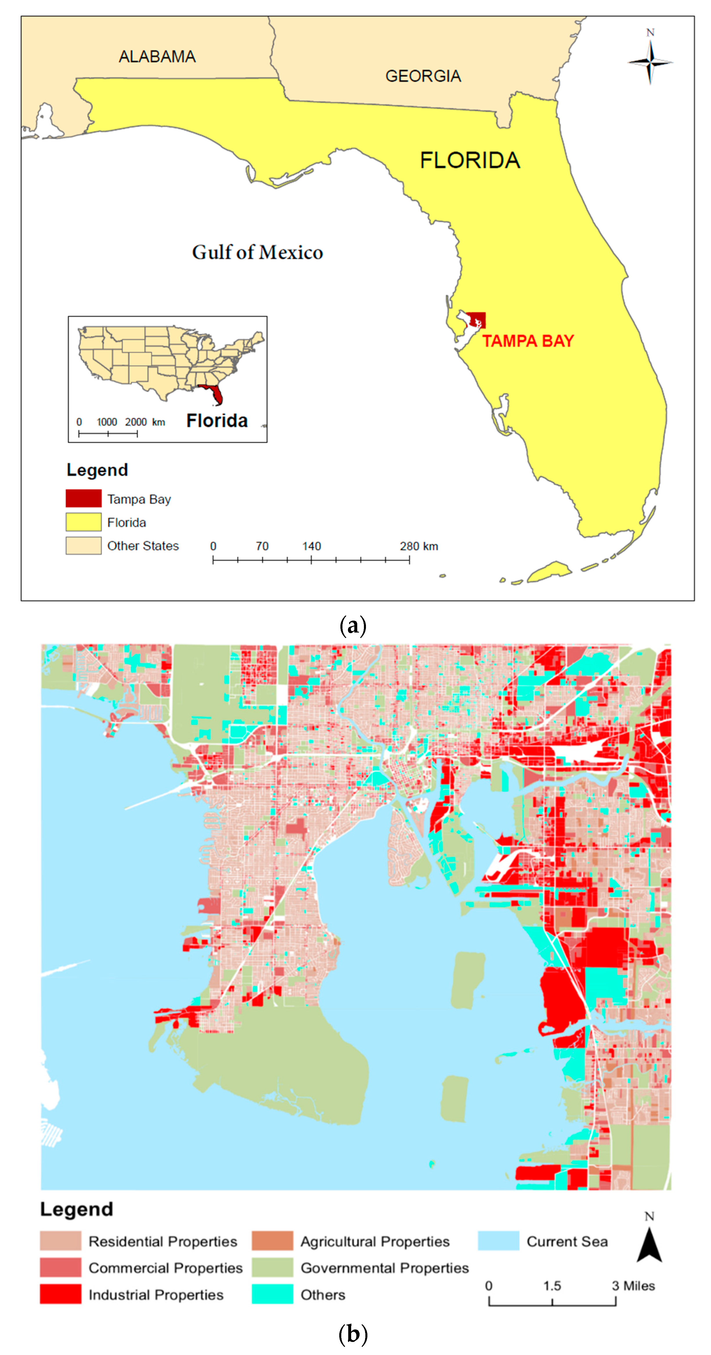
Tampa is located in Hillsborough County, west central Florida in USA. It is the largest city in Tampa Bay Area, near the Gulf of Mexico, and the fourth largest county in Florida. Tampa is well known to be vulnerable to sea-level rise due to its special location, high density of population, and increasingly condensed urban development. Even though Florida suffers several major hurricanes every year, the City of Tampa has not been hit by an extreme hurricane since 1921. For this reason, many tourists have been attracted to spend their vacations here, along with new immigrants who settle down in Tampa. According to the 2020 census, the current metro area population of Tampa is 2,877,000, and this number increased 1.23% compared to 2019. Last year, 27,000 new residents have put their roots in Hillsborough County. Such population booming makes Tampa Bay one of the country’s fastest growing regions in the U.S.; hence, it is critical for local governments to understand the economic costs through impacts to private properties, public infrastructure, the environment, and tourism. In Figure 1, we map and visualize the parcel-level property in Tampa, Florida.
Since 1946, the surrounding sea level has increased by 0.2 m [16]. Over the past decades, some researchers have investigated the sea level rise vulnerability of the Tampa Bay. For example, Fu et al. [17] used a spatial hedonic approach to estimating the economic cost in Tampa Bay region in future due to inundation caused by sea level rise. More recently, Fu and Peng [18] developed a conceptual vulnerability assessment framework to operationalize the full concept of vulnerability and test it through a case study in the Tampa Bay. Sherwood and Greening [19] analyzed potential impacts of sea level rise on Tampa Bay estuary and critical coastal habitats. With the increasing threat of climate change, the 2015 Peril of Flood Act mandates that municipalities in Florida need to consider sea-level rise in the coastal element of the comprehensive plan. However, because the mandate lacks specificity, a more recent study revealed an inconsistent compliance guidance provided by state agency staffs, and a top-down mandate strategy was suggested to spur sea-level rise planning [20].
2.2. Data
In this research, the following datasets will be used, including LIDAR-based digital elevation model, Global mean sea-level rise prediction data, and Tampa Property value datasets.
2.2.1. LIDAR-Based Digital Elevation Model (DEM)
This dataset is part of a series of DEMs produced for the National Oceanic and Atmospheric Administration Office (NOAA) for Coastal Management’s Sea-level Rise and Coastal Flooding Impacts Views (https://coast.noaa.gov/dataviewer, (accessed on 9 October 2021)). The DEM includes the best available LiDAR data known to exist at the time of DEM creation. The DEMs are “hydro flattened” such that water elevations are less than or equal to 0 m. The spatial resolution (cell size) of the raster DEM is 3 m, and the vertical accuracy is 10 cm. In this paper, a subset of data for the city of Tampa area was generated from a larger data set and includes all valid data within the requested geographic bounds.
2.2.2. Global Mean Sea-Level Rise Prediction Data
This paper will use the projection data of global mean sea-level rises [21], which use precise satellite altimeter data from the TOPEX/Poseidon (The Ocean Topography Experiment POSEIDON) Jason-1, Jason-2, and Jason-3 satellites that measure height above sea surface. We will use the measured global mean seal-level rise acceleration to obtain the sea-level rise in the future, in which short-term variability largely driven by volcanic eruptions (e.g., the eruption of Mount Pinatubo in 1991) and potential error drifts have been removed.
2.2.3. Property Value Datasets
This paper will use the parcel-level property tax GIS data to estimate the total values of properties, which are vulnerable to the coastal flooding. This dataset for the city of Tampa can be downloaded from Florida Department of Revenue (i.e., https://floridarevenue.com/property/, (accessed on 9 October 2021)), containing various information of individual property such as assessed value, land size and value, land use type, number of units, and so on, from property appraisers and tax collectors in local governments. These data are yearly updated, and we use the most recent data collected for the year of 2020.
2.3. Methods
To estimate the total economic cost of sea-level rise, those properties that will be located in flooding areas need to be identified. This can be underaken by comparing high-resolution digital surface elevations with the projected sea level. We consider an area as a possible flooding area when the elevation is lower than the sea level. Once all possible flooding areas are identified, a refining process is also performed to remove those areas that are not connected to the ocean, like valleys and lakes.
First, we will use the corrected global mean sea-level rise acceleration from a recent research [21] to obtain an approximated sea-level rise in the next several decades. Given the sea-level rise acceleration a and the initial sea-level rise rate , we are able to calculate the future sea levels, denoted by s, t years later using the following quadratic equation [21,22,23,24,25,26,27]:
Next, the following procedures will be performed to extract all possible areas to be flooded in the target area using ArcGIS:
- Given a sea level h and a DEM raster image D, one can produce a new raster image P to identify areas below the sea level in ArcGIS (Raster Calculator Toolbox) using the following formula,where d and p denote the variable for the DEM and the output raster image, respectively.
- Each individual pixel value in the raster image P is then reclassified using the reclassify tool in ArcGIS (Reclassification Toolbox) with the following equation:where g is the new cell value of the reclassified raster image G. This step aims to assign all unflooded areas as No Data, and only keep those areas whose elevation below the given sea level. Cells in D with values d which satisfy the condition d > h are assigned a value of No Data in G, and cells in D inundated by a rising sea are given a value of 1.
- However, it has been noticed that these flooding areas may include areas that have lower elevations than h but are not connected to the coastline, such as lakes, ponds, and valleys, in other words, these areas will not be flooded due to the sea-level rise, and they can be considered as anomalies to be removed prior to further processing. To do this, it is necessary to leverage coastlines as boundaries to select only those flooding areas that spatially intersect with the coastlines. To achieve this, this study will first convert the raster data G to the polygon feature class which consists of a list of polygons S = {}, each of which denotes the areas lower than the sea level, supposed that N polygons are detected. Given a coastline L provided by NOAA, one can check if each of N polygons intersects with L or not, and only keep those intersects, using the following equation:
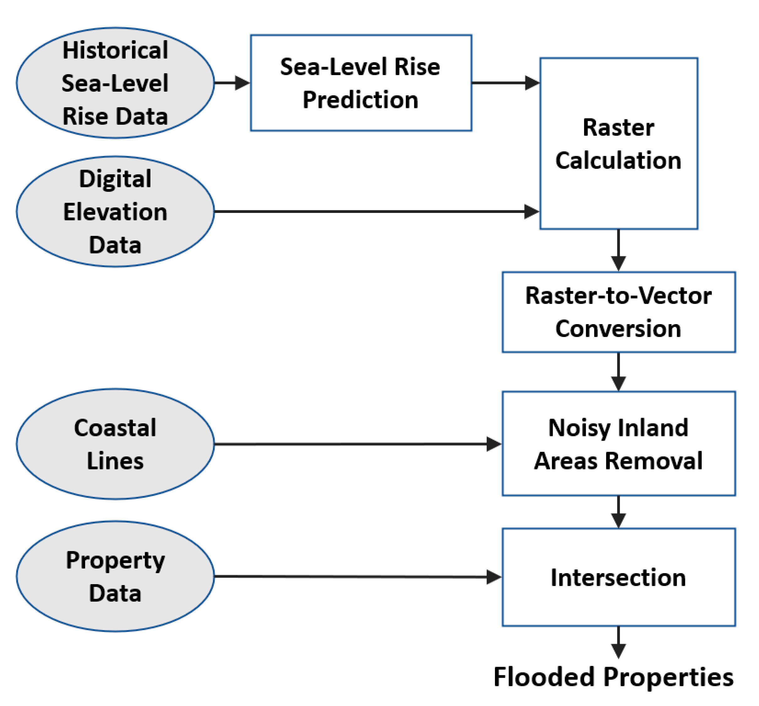
- The property value dataset provides house-level GIS information, and then one can identify all properties (e.g., houses, buildings, and other infrastructure) in flooding areas by spatially overlapping the property map with flooding areas. We summarize the data flow of our parcel-level flooding analysis in Figure 2. Each property has a land use code, indicating the type of property’s predominant use including residential, commercial, industrial, agricultural, institutional, governmental, and miscellaneous use. The detailed property value cost due to sea-level rise can be further analyzed for each type of property.
3. Results
Using the corrected sea-level rise acceleration 0.084 ± 0.025 mm/year2 obtained from 25-year precision satellite altimeter data, we can estimate future sea levels using Equation (1) coupled with an initial average climate-change-driven rate of sea-level rise of 2.9 mm/year. Table 1 illustrates the resulting predicted sea-level change from 2030 to 2150. It shows that the sea-level rise projections by the end of this century range from 46 cm for a low warming scenario (the best case) to 64 cm for a high warming scenario (the worst case). This projection is slightly higher than the one reported by the U.N.’s Intergovernmental Panel on Climate Change, where a sea-level rise of 41cm for low-end warming and 61 cm for high-end warming is projected [28].
In the rest of our analysis, we design three sea-level rise scenarios, i.e., low-end warming with mm/year2, medium-end warming with mm/year2, and high-end warming with mm/year2. We think the three scenarios will help enhance the understanding of the assessment of potentially flooded areas along the Tampa coastline and then identify and map all properties that are located in the areas under each scenario, respectively.
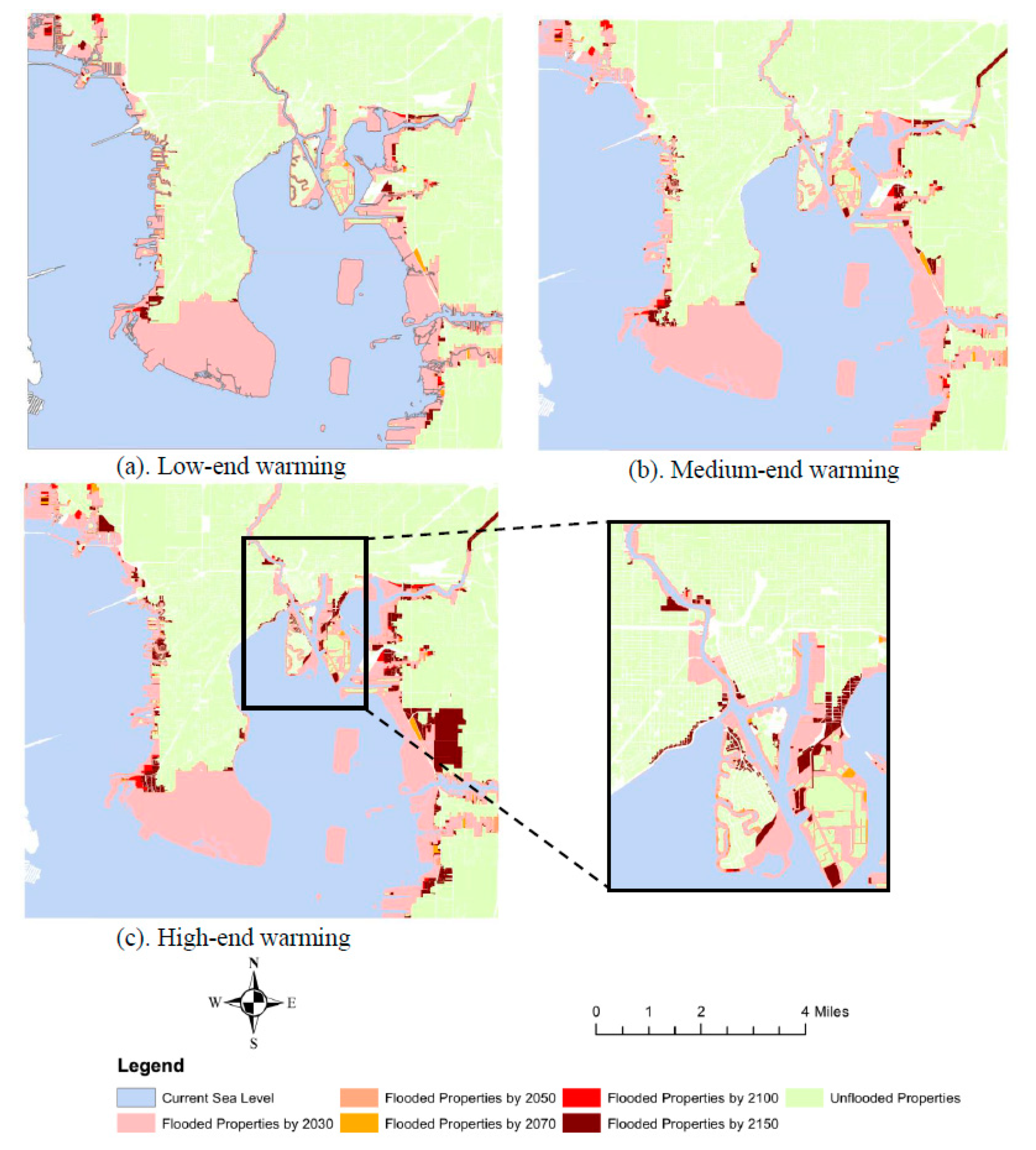
In Figure 3, we visualize all parcel-level properties in Tampa and those flooded from 2030 to 2150 under low-end, medium-end, and high-end warming scenarios in the absence of any protection. It shows that a large area in the south of Sun Bay South, particularly MacDill Air Force Base, and two major islands in Hillsborough Bay will be flooded by 2030. Table 2 summarizes the total amount of properties to be flooded and their associated land areas (in million square feet) due to sea-level rise in Tampa. It is predicted that there are around 4000 properties in total that will be flooded at the end of this century. This number would dramatically grow after 2100. For example, it will almost double (i.e., 7577 properties) by 2150 under the high-end warming scenario. Table 3 shows the total amount of flooded property value released by the Department of Revenue for the year of 2020. As shown in Table 3, this will lead to around 10 billion dollars property cost at the end of this century. It also shows an accelerated trend of property cost over time due to the sea-level rise. We would like to note that the costs shown in Table 3 are just direct costs which are only a fraction of total costs due to the sea-level rise. Additional indirect costs that are usually difficult to estimate would also include [29,30]: (1) the sectoral diffusion and inflation of damages (e.g., housing prices, demand surge, and company bankruptcy), (2) the response of economic shock (e.g., loss of invest confidence, and deepening inequality), and (3) financial and technical constraints that slow down reconstruction (e.g., availability of land for housing replacement).
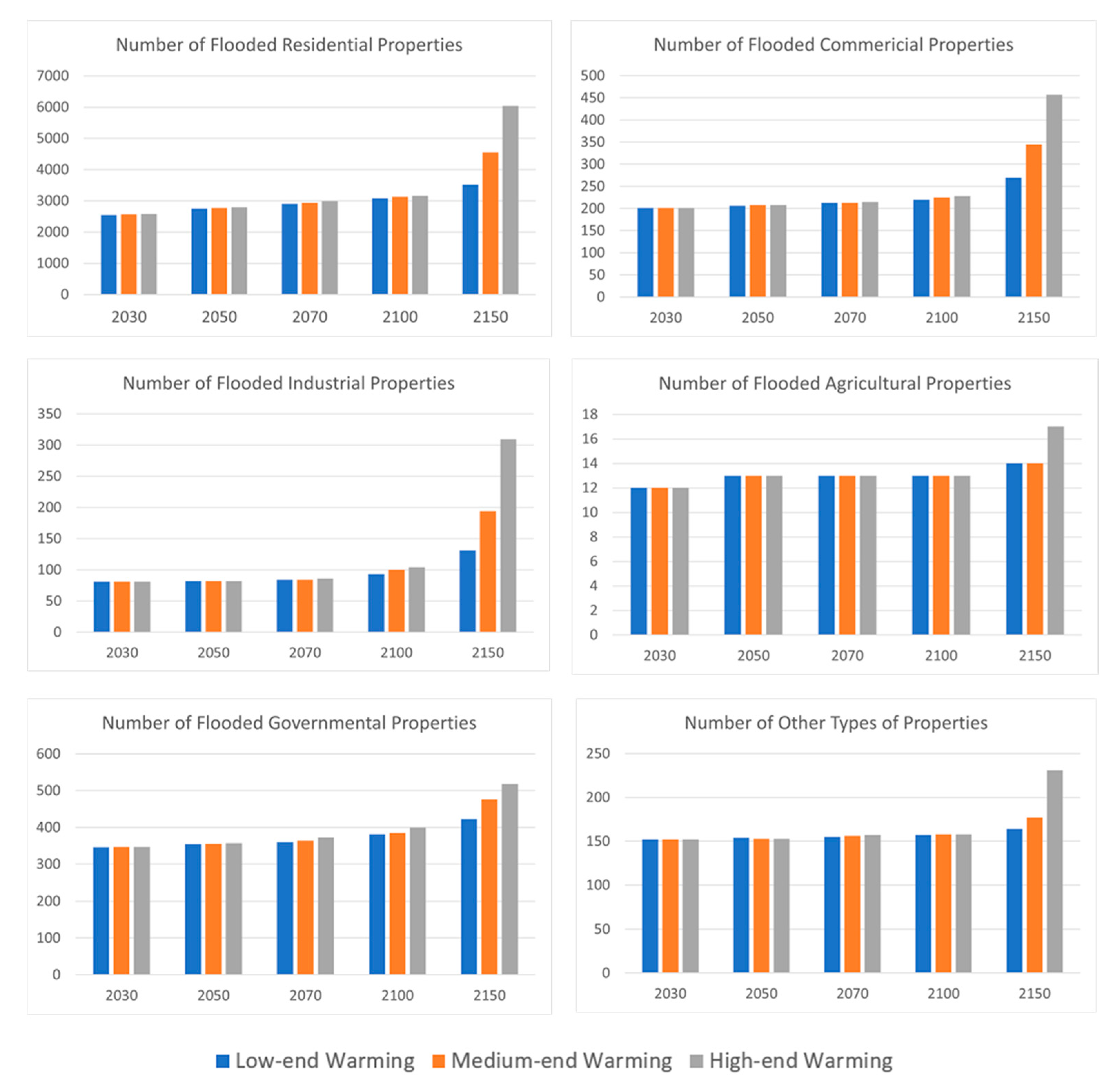
In addition to the total property value, we also analyze different types properties to be flooded under three warming scenarios. In particular, the following six categories of properties are considered: residential, commercial, industrial, agricultural, governmental, and other properties. Figure 4 shows the trend of the number of flooded properties under these six categories. It shows that residential property takes the largest portion of all flooded properties, indicating that sea-level rise will bring about the largest loss to those residents who live along coastline. In order to further understand the mostly affected area, we illustrate all residential, commercial and industrial properties (Figure 5, Figure 6 and Figure 7, respectively) that will be flooded in 2150 under the high-end warming scenario. From Figure 5, it can be shown that residential properties in neighborhoods of Bay Crest Park, Dana Shores, and Sunset Park have high risks of coastal flooding due to sea-level rise. Figure 6 shows that many commercial properties in Port Tampa City and Greater Palm River Point CDC will be flooded due to the sea-level rise. Since many industrial properties are also located in these two areas, Figure 6 shows that these two places have high risks of coastal flooding for industrial properties. The distribution of these mostly flooded areas can help local governments take specific adaptation and/or mitigation actions (e.g., using dikes or reinforcing buildings) to different areas so that the direct costs due to various sea levels can be significantly reduced.
4. Discussion
This study proposed three types of sea-level rise scenarios according to the climate change, using the high-resolution DEM data and the recently released high-precision sea level acceleration data, and then assessed the total land area and the cost of properties to be flooded due to the sea level rise in the city of Tampa, FL, USA. While this study only considers the current property value that might not reflect the exact cost for future sea flooding, it still provides meaningful guidance and insights to the impacts of sea level rise on urban assets and urban planning, which help governments and local communities design better planning strategies and mitigation actions. For example, the local government may design specific budgets, e.g., the amount of property tax to be used for mitigation, applications of different resources to specific communities within severe flooding areas, funding for building levees, dikes, and seawalls, or specific budget for vulnerable infrastructures that are identified in this study.
The findings of this study can be also used by governments, decision makers, and coastal planners to identify the most vulnerable population in sea-level rise flooding areas. It is also worth noting that the property cost we reported in this study is just a fraction of the total cost. Other costs, such as house appliances and furniture cost, property replacement cost, and possible cost of labor for moving, are difficult to estimate and are not considered in this study. In addition, this study does not consider the tide effects on the flooding property analysis. With different levels of tides, more lands and properties could be flooded due to the sea level rise plus extreme weather effects on tides such as hurricanes. The regular tide is caused by moon’s gravitational force, and the tide height is also subject to winds. This tide effect could be understood by adding a variation to the forecasted global sea level rise for a particular year.
While the Tampa Bay area is only studied in this research, the proposed work can be easily extended to other large coastal areas such as New York City and San Francisco, where the high-resolution LiDAR-based DEM data are available, and the spatial property maps and values are publicly available. The method and data flow developed in this paper can be helpful for other researchers and urban planners to analyze property impacts of sea-level rise flooding in other coastal regions.
However, we would also note that there are several uncertainties, including sea-level rise projection uncertainty, urban surface elevation uncertainty, and property value uncertainty, which are not considered in this paper and deserve further studies in future works. Firstly, the sea-level rise project uncertainty derives from the exclusion of local-level sea-level rise factors such as subsidence, erosion, and regional ocean currents; although, this paper considers three levels of global mean sea level rise (mean plus and minus standard derivation). The projection of local sea-level rise would provide a better estimation of coastal flood inundation. Secondly, the urban surface elevation uncertainty comes from the fact that the urban elevation will change with the urbanization process over time and the building of new infrastructure for flood mitigation. While it is hard to model such uncertainty, the inclusion of some simple models or assumptions would be also beneficial to understanding the impact of future sea-level rise flooding. Lastly, the property value uncertainty describes possible changes in property values in the future. Note that this paper only uses the latest property values for cost estimation. While this can help local governments and the public to have a direct understanding of the total economic cost if no further action is made, the estimation of future property values may provide more realistic economic costs related to the sea-level rise flooding.
5. Conclusions
This research examined the impact of sea-level rise on parcel-level properties in the city of Tampa, Florida. Rather than performing a global-scale analysis, this study focused on sea-level changes and associated urban property impacts in a typical coastal city. We used corrected sea-level rise estimates to predict sea levels in the future and identified potential areas of coastal flooding using a high-resolution LiDAR-based precise DEM. Coupled with parcel-level property value data, we further identified all properties with different types of use, which might be flooded due to the estimated sea level rise under three types of sea-level rise and climate change scenarios. These results enable the local governments and communities to better understand the risk of property damage due to sea-level rise induced by climate change. Therefore, our urban flooding risk analyses provide guidance and implications to local governments who could use it to adjust their approach to mitigation sea-level rise and climate change and reduce potential property damage costs. For example, the government may consider the percentage of property taxes every year to be assigned for building seawalls that could reduce the areas at risk of flooding. Our research in this paper focuses on the city of Tampa, and the spatial and temporal analyses can be easily extended by researchers or local governments to the major coastal cities in USA, such as New York City, San Francisco, and others coastal megacities across the world.
Author Contributions
Conceptualization, W.X. and Q.M.; methodology, W.X. and B.T.; software, W.X.; validation, W.X., Q.M., and B.T.; formal analysis, W.X.; investigation, W.X.; resources, B.T.; data curation, W.X.; writing—original draft preparation, W.X.; writing—review and editing, Q.M. and B.T.; visualization, W.X.; supervision, Q.M.; project administration, Q.M.; funding acquisition, Q.M. All authors have read and agreed to the published version of the manuscript.
Funding
This research received no external funding.
Conflicts of Interest
The authors declare no conflict of interest.
References
- Oliver-Smith, A. Sea Level Rise and the Vulnerability of Coastal Peoples: Responding to the Local Challenges of Global Climate Change in the 21st Century; UNU-EHS: Bonn, Germany, 2009; Available online: http://collections.unu.edu/eserv/UNU:1861/pdf4097.pdf (accessed on 9 October 2021).
- Hinkel, J.; Lincke, D.; Vafeidis, A.; Perrette, M.; Nicholls, R.; Tol, R.; Marzeion, B.; Fettweis, X.; Ionescu, C.; Levermann, A. Coastal flood damage and adaptation costs under 21st century sea-level rise. Proc. Natl. Acad. Sci. USA 2014, 111, 3292–3297. [Google Scholar] [CrossRef] [Green Version]
- Leatherman, S.P. Social and economic costs of sea level rise. In International Geophysics; Academic Press: Cambridge, MA, USA, 2001; Volume 75, pp. 181–223. [Google Scholar]
- Desmet, K.; Kopp, R.E.; Kulp, S.A.; Nagy, D.K.; Oppenheimer, M.; Rossi-Hansberg, E.; Strauss, B.H. Evaluating the Economic Cost of Coastal Flooding. Macroeconomics 2021, 13, 444–486. [Google Scholar] [CrossRef]
- Hossain, M.; Meng, Q. A Multi-Decadal Spatial Analysis of Demographic Vulnerability to Urban Flood: A Case Study of Birmingham City, USA. Sustainability 2020, 12, 9139. [Google Scholar] [CrossRef]
- Hossain, M.K.; Meng, Q. A thematic mapping method to assess and analyze potential urban hazards and risks caused by flooding. Comput. Environ. Urban Syst. 2020, 79, 101417. [Google Scholar] [CrossRef]
- Rifat, S.; Liu, W. Measuring Community Disaster Resilience in the Conterminous Coastal United States. ISPRS Int. J. Geo-Inf. 2020, 9, 469. [Google Scholar] [CrossRef]
- Balk, D.; Montgomery, M.R.; McGranahan, G.; Kim, D.; Mara, V.; Todd, M.; Buettner, T.; Dorélien, A. Mapping urban settlements and the risks of climate change in Africa, Asia and South America. Popul. Dyn. Clim. Chang. 2009, 80, 103. [Google Scholar]
- McGranahan, G.; Balk, D.; Anderson, B. The rising tide: Assessing the risks of climate change and human settlements in low elevation coastal zones. Environ. Urban. 2007, 19, 17–37. [Google Scholar] [CrossRef]
- FitzGerald, D.M.; Fenster, M.S.; Argow, B.A.; Buynevich, I.V. Coastal Impacts Due to Sea-Level Rise. Annu. Rev. Earth Planet. Sci. 2008, 36, 601–647. [Google Scholar] [CrossRef] [Green Version]
- Strauss, B.; Tebaldi, C.; Ziemlinski, R. Sea level rise, storms & global warming’s threat to the US coast. Clim. Cent. 2012. Available online: https://research.fit.edu/media/site-specific/researchfitedu/coast-climate-adaptation-library/united-states/national/us---other-national-reports/Strauss-et-al.-2012.-US-Coasts-SLR--Storms.pdf (accessed on 14 March 2012).
- Neumann, B.; Vafeidis, A.T.; Zimmermann, J.; Nicholls, R.J. Future coastal population growth and exposure to sea-level rise and coastal flooding-a global assessment. PLoS ONE 2015, 10, e0118571. [Google Scholar] [CrossRef] [Green Version]
- Jevrejeva, S.; Jackson, L.P.; Grinsted, A.; Lincke, D.; Marzeion, B. Flood damage costs under the sea level rise with warming of 1.5 °C and 2 °C. Environ. Res. Lett. 2018, 13, 074014. [Google Scholar] [CrossRef] [Green Version]
- Kulp, S.A.; Strauss, B.H. New elevation data triple estimates of global vulnerability to sea-level rise and coastal flooding. Nat. Commun. 2019, 10, 4844. [Google Scholar] [CrossRef] [PubMed] [Green Version]
- Xian, G.; Crane, M. Assessments of urban growth in the Tampa Bay watershed using remote sensing data. Remote Sens. Environ. 2005, 97, 203–215. [Google Scholar] [CrossRef]
- Fortado, L. Tampa Bay Cities Prepare for Rising Sea Levels and Storm Risk. Financial Times. 20 September 2019. Available online: https://www.ft.com/content/780ca792-b7a8-11e9-8a88-aa6628ac896c (accessed on 2 October 2021).
- Fu, X.; Song, J.; Sun, B.; Peng, Z.-R. “Living on the edge”: Estimating the economic cost of sea level rise on coastal real estate in the Tampa Bay region, Florida. Ocean Coast. Manag. 2016, 133, 11–17. [Google Scholar] [CrossRef]
- Fu, X.; Peng, Z.-R. Assessing the sea-level rise vulnerability in coastal communities: A case study in the Tampa Bay Region, US. Cities 2019, 88, 144–154. [Google Scholar] [CrossRef]
- Sherwood, E.T.; Greening, H.S. Potential Impacts and Management Implications of Climate Change on Tampa Bay Estuary Critical Coastal Habitats. Environ. Manag. 2013, 53, 401–415. [Google Scholar] [CrossRef]
- Holmes, T.J.; Butler, W.H. Implementing a mandate to plan for sea level rise: Top-down, bottom-up, and middle-out actions in the Tampa Bay region. J. Environ. Plan. Manag. 2021, 64, 2214–2232. [Google Scholar] [CrossRef]
- Nerem, R.S.; Beckley, B.D.; Fasullo, J.T.; Hamlington, B.D.; Masters, D.; Mitchum, G.T. Climate-change–driven accelerated sea-level rise detected in the altimeter era. Proc. Natl. Acad. Sci. USA 2018, 115, 2022–2025. [Google Scholar] [CrossRef] [Green Version]
- Nerem, R.S.; Chambers, D.; Choe, C.; Mitchum, G.T. Estimating Mean Sea Level Change from the TOPEX and Jason Altimeter Missions. Mar. Geodesy 2010, 33, 435–446. [Google Scholar] [CrossRef]
- Church, J.A.; White, N.J. A 20th century acceleration in global sea-level rise. Geophys. Res. Lett. 2006, 33. [Google Scholar] [CrossRef]
- Houston, J.R.; Dean, R.G. Sea-level acceleration based on US tide gauges and extensions of previous global-gauge analyses. J. Coast. Res. 2011, 27, 409–417. [Google Scholar]
- Douglas, B.C. Global sea level acceleration. J. Geophys. Res. Space Phys. 1992, 97, 12699. [Google Scholar] [CrossRef] [Green Version]
- Dieng, H.B.; Cazenave, A.; Meyssignac, B.; Ablain, M. New estimate of the current rate of sea level rise from a sea level budget approach. Geophys. Res. Lett. 2017, 44, 3744–3751. [Google Scholar] [CrossRef]
- Taherkhani, M.; Vitousek, S.; Barnard, P.L.; Frazer, N.; Anderson, T.R.; Fletcher, C.H. Sea-level rise exponentially increases coastal flood frequency. Sci. Rep. 2020, 10, 6466. [Google Scholar] [CrossRef]
- IPCC. AR5 Synthesis Report: Climate Change 2014. 2014. Available online: https://www.ipcc.ch/report/ar5/syr/ (accessed on 2 October 2021).
- Galbusera, L.; Giannopoulos, G. On input-output economic models in disaster impact assessment. Int. J. Disaster Risk Reduct. 2018, 30, 186–198. [Google Scholar] [CrossRef]
- Hallegatte, S.; Henriet, F.; Corfee-Morlot, J. The economics of climate change impacts and policy benefits at city scale: A conceptual framework. Clim. Chang. 2010, 104, 51–87. [Google Scholar] [CrossRef]
Figure 1.
Parcel-level property map of the studied area: (a) The location of Tampa Bay, Hillsborough County, Florida, (b) Six types of properties.
Figure 1.
Parcel-level property map of the studied area: (a) The location of Tampa Bay, Hillsborough County, Florida, (b) Six types of properties.

Figure 2.
Data flow of our parcel-level flooding analysis.

Figure 3.
Flooded properties due to sea-level rise in Tampa: (a) low-end warming, (b) medium-end warming, and (c) high-end warming.
Figure 3.
Flooded properties due to sea-level rise in Tampa: (a) low-end warming, (b) medium-end warming, and (c) high-end warming.

Figure 4.
Number of flooded properties for different categories, where x-axis denotes the year and y-axis denotes the number of properties for the specific category.
Figure 4.
Number of flooded properties for different categories, where x-axis denotes the year and y-axis denotes the number of properties for the specific category.

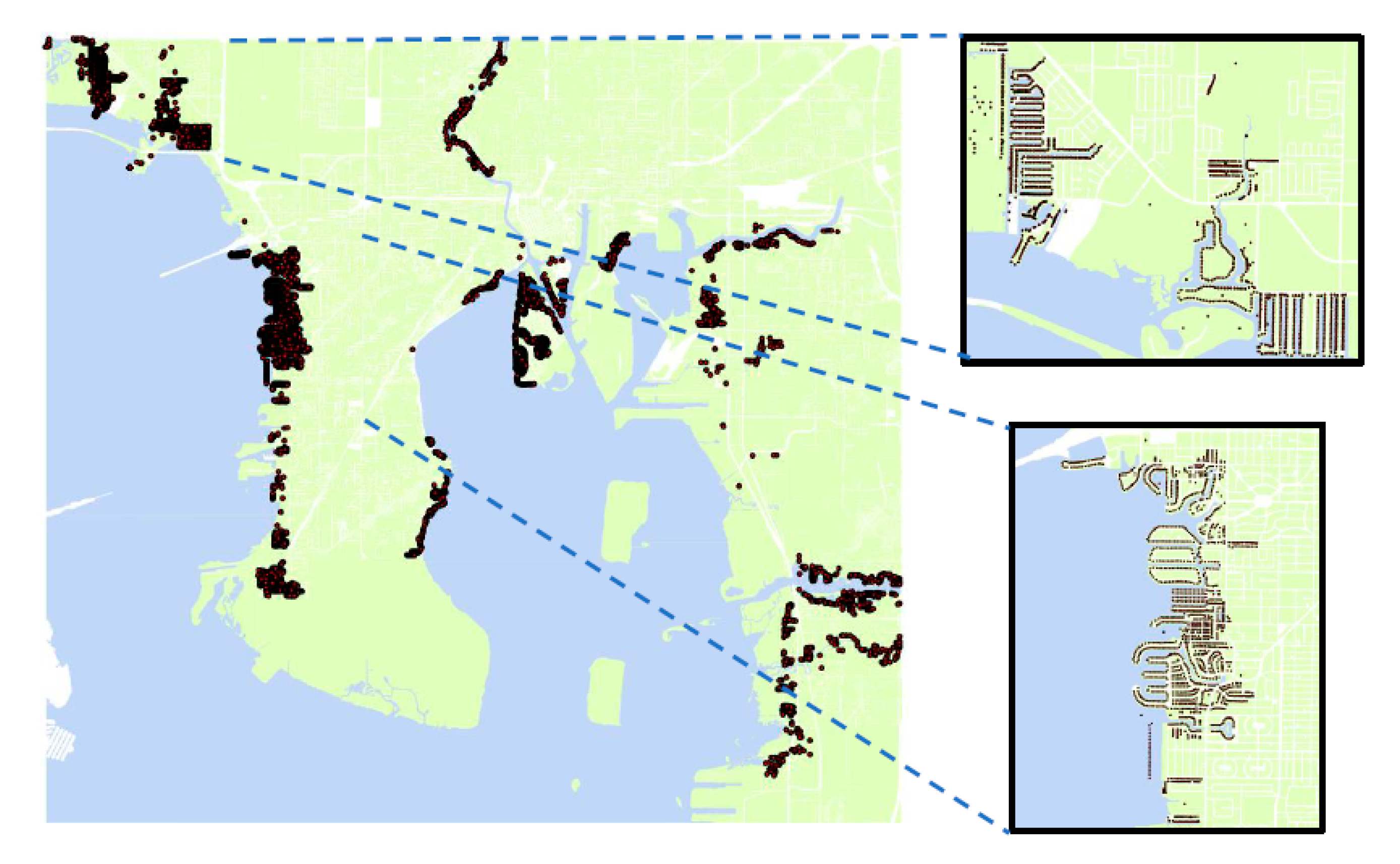
Figure 5.
Flooded residential properties by 2150 in the high-end warming scenario. The most two flooded areas are detailed in the right two subfigures. Each black dot denotes one property to be flooded due to sea level rise.
Figure 5.
Flooded residential properties by 2150 in the high-end warming scenario. The most two flooded areas are detailed in the right two subfigures. Each black dot denotes one property to be flooded due to sea level rise.

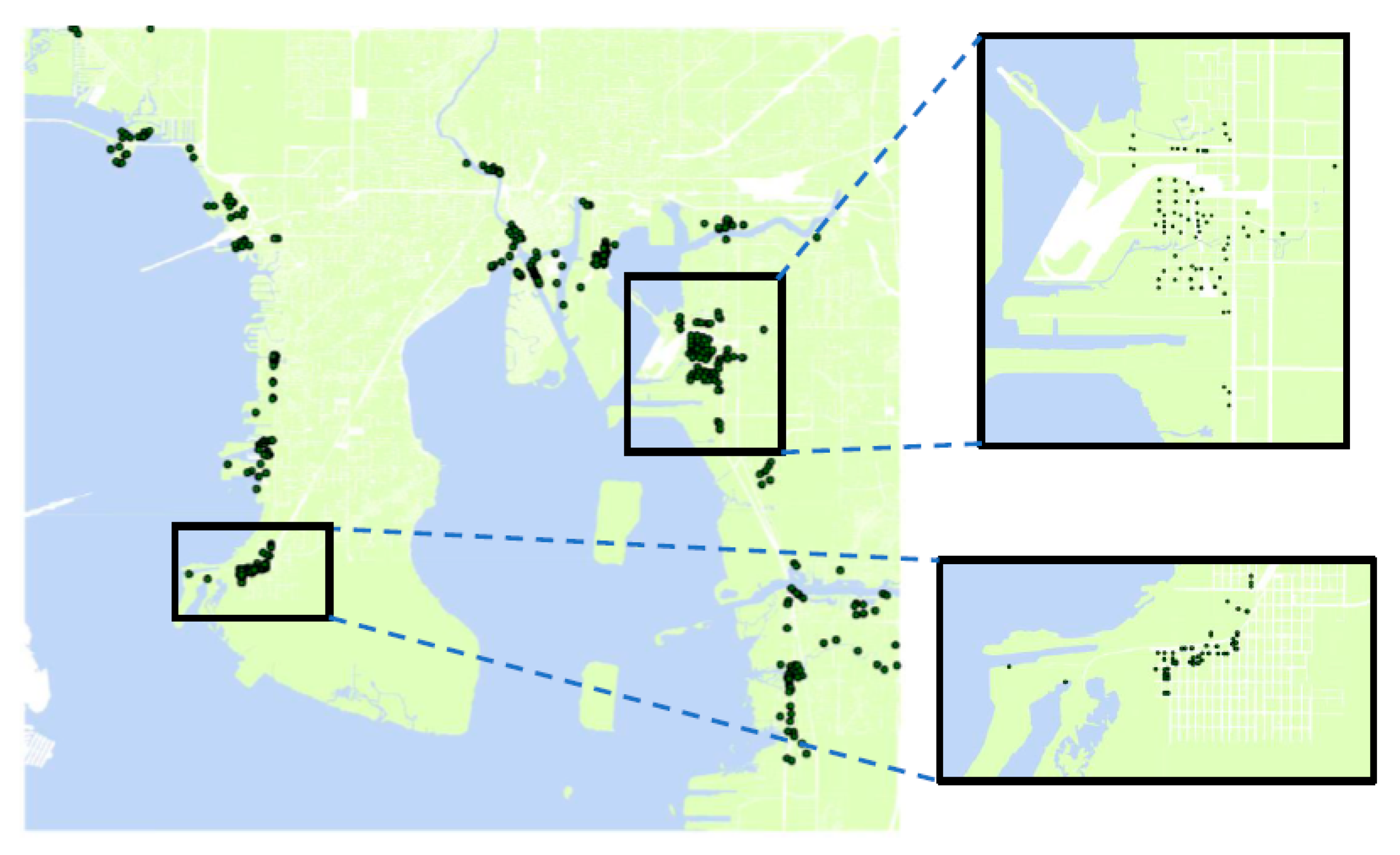
Figure 6.
Flooded commercial properties by 2150 in the high-end warming scenario. The most two flooded areas are detailed in the right two subfigures. Each black dot denotes one property to be flooded due to sea level rise.
Figure 6.
Flooded commercial properties by 2150 in the high-end warming scenario. The most two flooded areas are detailed in the right two subfigures. Each black dot denotes one property to be flooded due to sea level rise.

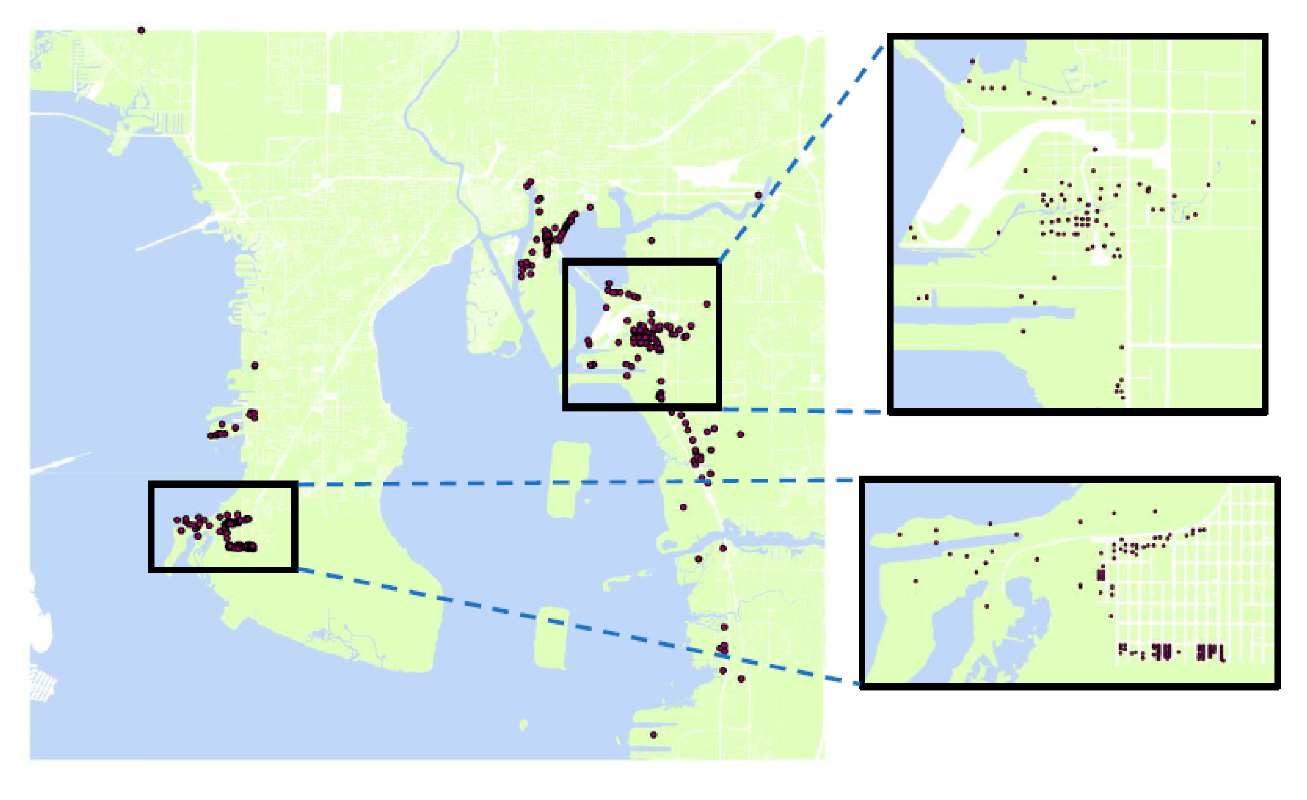
Figure 7.
Flooded industrial properties by 2150 in the high-end warming scenario. The most two flooded areas are detailed in the right two subfigures. Each black dot denotes one property to be flooded due to sea level rise.
Figure 7.
Flooded industrial properties by 2150 in the high-end warming scenario. The most two flooded areas are detailed in the right two subfigures. Each black dot denotes one property to be flooded due to sea level rise.


Table 1.
Predicted Sea-Level Rise (years 2030–2150) Using Corrected Sea-Level Rise Acceleration of 0.084 ± 0.025mm/year2 with an Initial Rate of 2.9 mm/year.
Table 1.
Predicted Sea-Level Rise (years 2030–2150) Using Corrected Sea-Level Rise Acceleration of 0.084 ± 0.025mm/year2 with an Initial Rate of 2.9 mm/year.
| Year | 2030 | 2050 | 2070 | 2100 | 2150 |
|---|---|---|---|---|---|
| Sea-level Rise (cm) mm/year2 | 5.01 | 13.76 | 24.87 | 45.96 | 92.91 |
| Sea-level Rise (cm) mm/year2 | 5.29 | 15.29 | 28.66 | 55 | 115.7 |
| Sea-level Rise (cm) mm/year2 | 5.58 | 16.83 | 32.44 | 64.03 | 138.48 |
Table 2.
Total amount of flooded properties and their total land area (million square feet) (years 2030–2150).
Table 2.
Total amount of flooded properties and their total land area (million square feet) (years 2030–2150).
| Years | 2030 | 2050 | 2070 | 2100 | 2150 | |
|---|---|---|---|---|---|---|
| Low-end Warming | Total Amount | 3334 | 3563 | 3724 | 3946 | 4518 |
| Total Area | 15,419 | 15,430 | 15,465 | 15,649 | 15,861 | |
| Medium-end Warming | Total Amount | 3357 | 3586 | 3767 | 4005 | 5753 |
| Total Area | 15,420 | 15,457 | 15,468 | 15,663 | 16,243 | |
| High-end Warming | Total Amount | 3371 | 3605 | 3827 | 4064 | 7577 |
| Total Area | 15,420 | 15,458 | 15,471 | 15,680 | 16,362 |
Table 3.
Total value of flooded properties in million dollars (years 2030–2150).
| Years | 2030 | 2050 | 2070 | 2100 | 2150 |
|---|---|---|---|---|---|
| Low-end Warming | 8347 | 8686 | 8914 | 9141 | 10,333 |
| Medium-end Warming | 8386 | 8768 | 8961 | 9258 | 11,355 |
| High-end Warming | 8400 | 8785 | 8999 | 9332 | 12,256 |
Publisher’s Note: MDPI stays neutral with regard to jurisdictional claims in published maps and institutional affiliations. |
© 2021 by the authors. Licensee MDPI, Basel, Switzerland. This article is an open access article distributed under the terms and conditions of the Creative Commons Attribution (CC BY) license (https://creativecommons.org/licenses/by/4.0/).
Share and Cite
MDPI and ACS Style
Xie, W.; Tang, B.; Meng, Q. The Impact of Sea-Level Rise on Urban Properties in Tampa Due to Climate Change. Water 2022, 14, 13. https://doi.org/10.3390/w14010013
AMA Style
Xie W, Tang B, Meng Q. The Impact of Sea-Level Rise on Urban Properties in Tampa Due to Climate Change. Water. 2022; 14(1):13. https://doi.org/10.3390/w14010013
Chicago/Turabian StyleXie, Weiwei, Bo Tang, and Qingmin Meng. 2022. "The Impact of Sea-Level Rise on Urban Properties in Tampa Due to Climate Change" Water 14, no. 1: 13. https://doi.org/10.3390/w14010013
Note that from the first issue of 2016, this journal uses article numbers instead of page numbers. See further details here.