
Integrated Approach to Quantify the Impact of Land Use and Land Cover Changes on Water Quality of Surma River, Sylhet, Bangladesh


1
Department of Geography and Environment, Shahjalal University of Science and Technology, Sylhet 3114, Bangladesh
2
Department of Civil and Environmental Engineering, Shahjalal University of Science and Technology, Sylhet 3114, Bangladesh
3
Department of Geoscience, Florida Atlantic University, Boca Raton, FL 33431, USA
4
Institute for Global Environmental Strategies, Hayama, Kanagawa 240-0115, Japan
*
Author to whom correspondence should be addressed.
Water 2022, 14(1), 17; https://doi.org/10.3390/w14010017
Submission received: 16 November 2021
/
Revised: 17 December 2021
/
Accepted: 19 December 2021
/
Published: 22 December 2021
(This article belongs to the Special Issue Water Resource Management through the Lens of Planetary Health Approach)
Abstract
:This study aims to assess the impacts of land use and land cover (LULC) changes on the water quality of the Surma river in Bangladesh. For this, seasonal water quality changes were assessed in comparison to the LULC changes recorded from 2010 to 2019. Obtained results from this study indicated that pH, electrical conductivity (EC), and total dissolved solids (TDS) concentrations were higher during the dry season, while dissolved oxygen (DO), 5-day biological oxygen demand (BOD5), temperature, total suspended solids (TSS), and total solids (TS) concentrations also changed with the season. The analysis of LULC changes within 1000-m buffer zones around the sampling stations revealed that agricultural and vegetation classes decreased; while built-up, waterbody and barren lands increased. Correlation analyses showed that BOD5, temperature, EC, TDS, and TSS had a significant relationship (5% level) with LULC types. The regression result indicated that BOD5 was sensitive to changing waterbody (predictors, R2 = 0.645), temperature was sensitive to changing waterbodies and agricultural land (R2 = 0.889); and EC was sensitive to built-up, vegetation, and barren land (R2 = 0.833). Waterbody, built-up, and agricultural LULC were predictors for TDS (R2 = 0.993); and waterbody, built-up, and barren LULC were predictors for TSS (R2 = 0.922). Built-up areas and waterbodies appeared to have the strongest effect on different water quality parameters. Scientific finding from this study will be vital for decision makers in developing more robust land use management plan at the local level.
1. Introduction
Water is a vital resource for the maintenance of life, ecological functioning, biological diversity, and social well-being. Despite its importance for life, in recent decades, excessive human land use has severely harmed the quality and quantities of available water resources [1]. In particular, it is well known that rivers function as integrators of land-water connections, receiving pollutants from the surrounding landscapes [2], and river water quality could be negatively impacted. Surma River, an important river in Bangladesh, has been collecting pollutants from a wide variety of point and non-point sources along its course from agricultural wastes, industrial effluents, menage wastes, and municipal sewage [3]. Due to population growth, urbanization, and industrialization, the surrounding landscape of the Surma river has been changing, and the riverside has experienced tremendous development in terms of commercial, human settlement, and industrial development. The population and urban sprawl have adverse effects on the quality of the Surma river water; the increased urban area is responsible for generating large amounts of nonpoint source pollution through runoff and degraded the river water quality.
Land use and land cover (LULC) within the immediate environments of a waterbody have a direct impact on the physicochemical and microbiological properties of water, and such impact varies with the type, extent, location of human land uses, and the inputs from the watershed. Water quality problems arise when the type and extent of human land use exceed the natural ability of the watershed to mitigate accumulated land-use-related stress [4]. Numerous studies have shown that human activities lead to landscape pattern changes, which in turn had significant impacts on the conditions of river water [2,5,6]. LULC change, especially urbanization, has a major impact on hydrology, affecting water quality and quantity on a range of spatial and temporal scales [7,8]. Zhu [9] found that water quality degrading was particularly affected by alteration from farmland to commercial and residential land, and the expansion in an urban area causes streamflow increase, carrying more sediment, bank erosion, and nutrients in streams. Hossain [10] reported that water quality variables are correlated with LULC change. As a consequence of the spatiotemporal LULC change, the concentration of diffuse pollutants in streams varies as well as vegetation types, and watershed climate are responsible for stream water quality change.
Landscape pattern has a complex, space- and scale-dependent effect on water quality [11,12], and different landscape characteristics play different roles in receiving water at different spatial scales varying from the local to eco-regional scales [13]. Bhaduri et al. [7] noted that the most significant human impacts on the hydrologic system and water resources are caused by land-use changes on local, regional, and global scales, driven by a rise in urban areas. Pollution from nonpoint sources (NPS) is a challenging problem to solve as it comes from a variety of origins difficult to pinpoint, and it occurs in a variety of environments; however, Geographical Information Systems (GIS) software provides a more comprehensive description of land cover patterns and the spatial distribution of NPS pollution [14] and has been commonly used. To explore the landscape pattern’s impacts on the lakes and rivers water quality several studies have been conducted [15,16], and it seems that the riparian buffer zone landscape patterns are more powerful in explaining water quality variations [17]. Land use types have an influence on surface water quality which can be analyzed by using statistical methods, remote sensing (RS), and geographic information system (GIS) [18,19,20,21]. Li et al. [12] stated that in riparian zones, the landscape category has a significant impact on water quality, and the alterations in the landscape through urban spread have put a lot of pressure on undeveloped land. Ribeiro et al. [22] found that water quality was worse in the sub-basin, also characterized by the presence of more agriculture, permanent conservation area, lesser natural forest, and a greater drainage area; however, the existence of agriculture negatively affect water quality in the riparian area. As proven by numerous studies, water quality is closely correlated to landscape pattern, which includes the landscape structure and spatial configuration [23,24,25,26].
So, it is essential to find out the spatiotemporal and future potential effect on water quality by LULC change. Therefore, this study examines the LULC change in the riparian buffer zone of the Surma river, over the period 2010 to 2019. The seasonal surface water quality variation is analyzed next. The study aims to assess the impacts of land use and land cover (LULC) changes on the Surma river surface water quality.
The outcomes of this study will make it helpful to acquire sustainability of land and water resources. Additionally, it will facilitate other researchers’ pursuit of studies about LULC change impact on water quality in the study area and similar regions.
2. Materials and Methods
2.1. Design of the Study
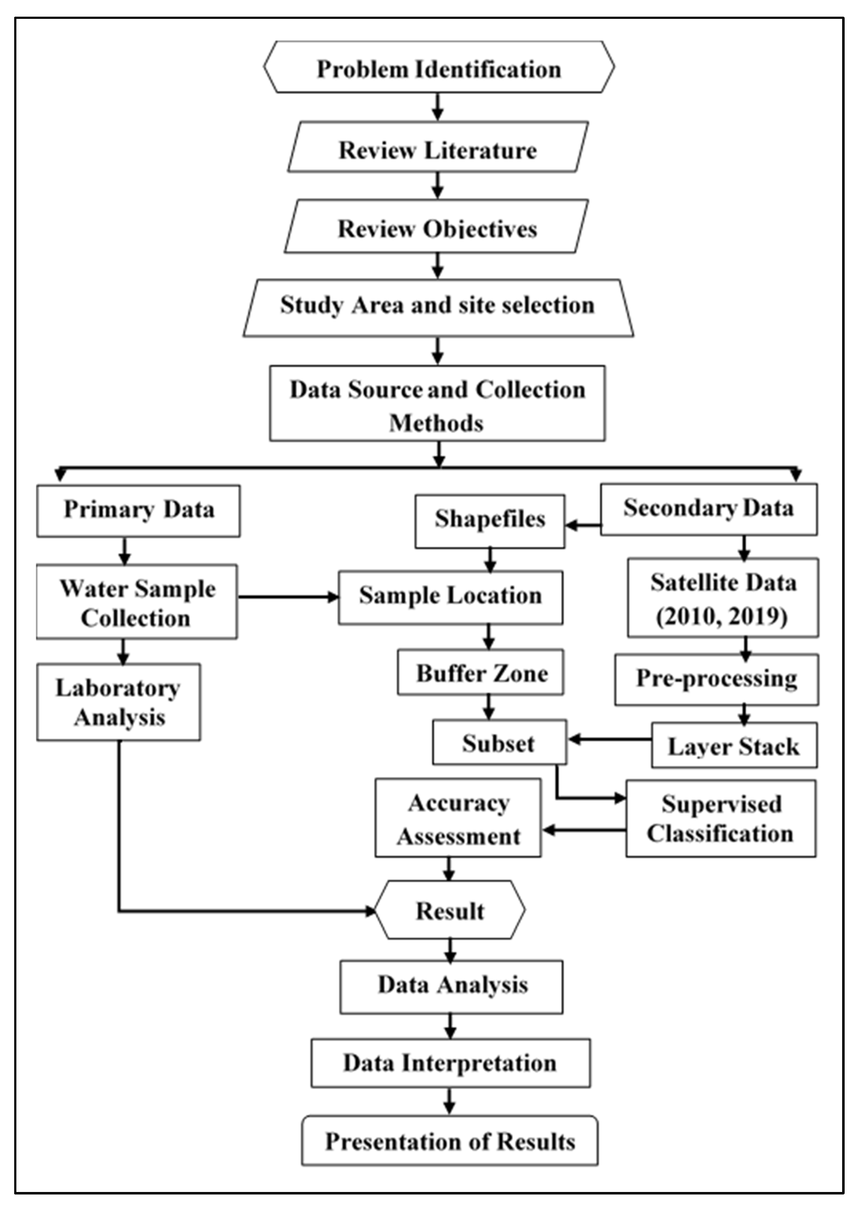
We have conducted this research work systematically and scientifically; the major methods and techniques, which were followed very carefully, are illustrated in Figure 1.
2.2. Study Area
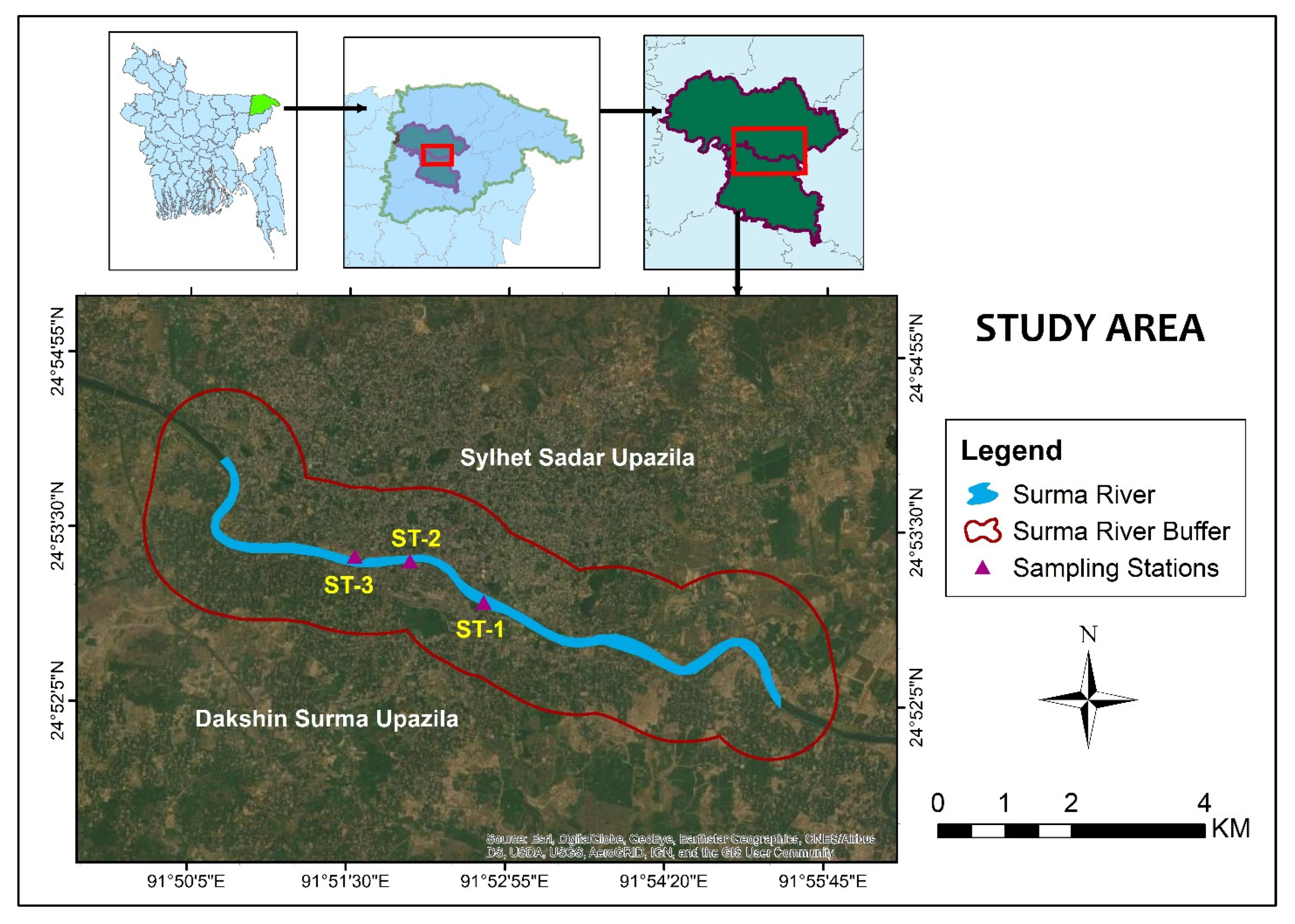
In Bangladesh, Surma is an important river, as a part of the Surma–Meghna river system, which originates when the Barak River in northeastern India and then splits into two branches at the Bangladesh border as the Surma (a northern branch that flows west and then runs southwest to the town of Sylhet) and the Kushiyara rivers [27]. Sylhet Sadar Upazila and Dakshin Surma Upazila are two Upazilas of the Sylhet district, which are located in the country’s north-eastern region. Upazila is an administrative region in Bangladesh, equivalent to a county of Western countries. The study was conducted in the Surma river portion, situated between Sylhet Sadar Upazila and Dakshin Surma Upazila land, extending 1000 m toward both sides of the riverbank. It is situated between 24°51′39.1″ N to 24°54′37.07″ N latitude and between 91°49′40.9″ E to 91°55′51.9″ E longitude (Figure 2).
2.3. Water Sampling and Analytical Methods
This study considered both primary and secondary data on water quality. Water quality data for the dry and wet season of 2010 was collected from the Department of Environment (DoE), Sylhet Divisional Office, Sylhet, Bangladesh.
Water samples were collected from three (ST-1, ST-2, and ST-3) separate Surma river sampling stations, each with a different geographic location, as shown in Table 1. Following the collection, water samples were kept in an ice box and bought to the laboratory. Sampling was performed in the dry season (2019) and the wet season (2019).
Eight water quality parameters were selected, including dissolved oxygen (DO), 5-day biological oxygen demand (BOD5), pH, electrical conductivity (EC), temperature, total suspended solids (TSS), total dissolved solids (TDS), and total solids (TS). All the water samples of 2019 were analyzed in the Water Supply and Sewerage Engineering Laboratory of Civil and Environmental Engineering Department, and Environmental Laboratory of Geography and Environment Department, Shahjalal University of Science and Technology, Sylhet, Bangladesh. DO and BOD5 were measured by the Winkler titration method, pH and temperature were measured by electrometric methods (pH meter, HANNA-HI 9125), electrical conductivity (EC) was measured using an EC meter (HANNA-HI 98192); and TDS, TSS, and TS were measured in the laboratory following standard methods [28].
2.3.1. LULC Change Analysis
For land use and land cover (LULC) change analysis, satellite images of 2010 (Landsat 5 Thematic Mapper) and 2019 (Sentinel 2 MSI), acquired from the United States Geological Survey (USGS), were used to produce LULC classification maps for both years using remote sensing (ERDAS IMAGINE 2014) and geographic information system (ArcGIS 10.8) software. LULC classes are categorized into five major categories including, waterbody (river, canals, pond, lakes, reservoirs), built-up (urban areas, human settlements, road networks. Commercial and industrial areas), agricultural land (cropland, pasture, herb, shrub, fallow land, permeable surface), vegetation (canopy, mixed forest, evergreen forest), and barren land (bare soil, sand, rocks without vegetation). Satellite image preprocessing, as well as geometrical rectification, registration of image, corrections viz. atmospheric and radiometric, were conducted by ERDAS IMAGINE 2014. Supervised classification was conducted to create LULC maps [29]. Accuracy assessment was conducted, indicating that the overall classification accuracy of the 2010 image was 81.65% and a kappa statistics of 0.7524, and overall classification accuracy of the 2019 image was 94.50% and kappa statistics of 0.9024, indicating a very good accuracy of the LULC map. By using ArcGIS 10.8 software, land uses composition within the 1000-m buffer zones around the sampling stations was extracted from the LULC map. A 1000-m buffer scale is stronger than smaller scales in explaining land-use types and their water quality relations [30]. Percentages of these broad LULC types were used to examine the relationship between water quality parameters and LULC types.
2.3.2. Statistical Analyses
Descriptive statistics were used to explain the general characteristics of LULC and water quality parameters. Karl Pearson’s correlation analysis was used to determine correlations between LULC patterns percentage and water quality parameters (WQPs) at statistical significance at a 5% level. Backward stepwise regression analysis was used to identify the relationship between the percentage of land usage composition within the 1000-m buffer zone and water quality properties. WQPs showing significant correlations with LULC types were considered for the backward stepwise regression analysis. In regression analysis, water quality parameters (BOD5, temperature, EC, TDS, and TSS) were considered dependent variables, while LULC types (waterbody, built-up, vegetation, agricultural land, and barren land) were treated as independent variables. To identify the best combination of land uses for water quality estimation regression equations were compared with R2 values (value closer to one indicates a greater accuracy of the model). The Statistical Packages for Social Science (IBM SPSS Statistics 20) for windows was used to perform all statistical analyses.
3. Results
3.1. Water Quality
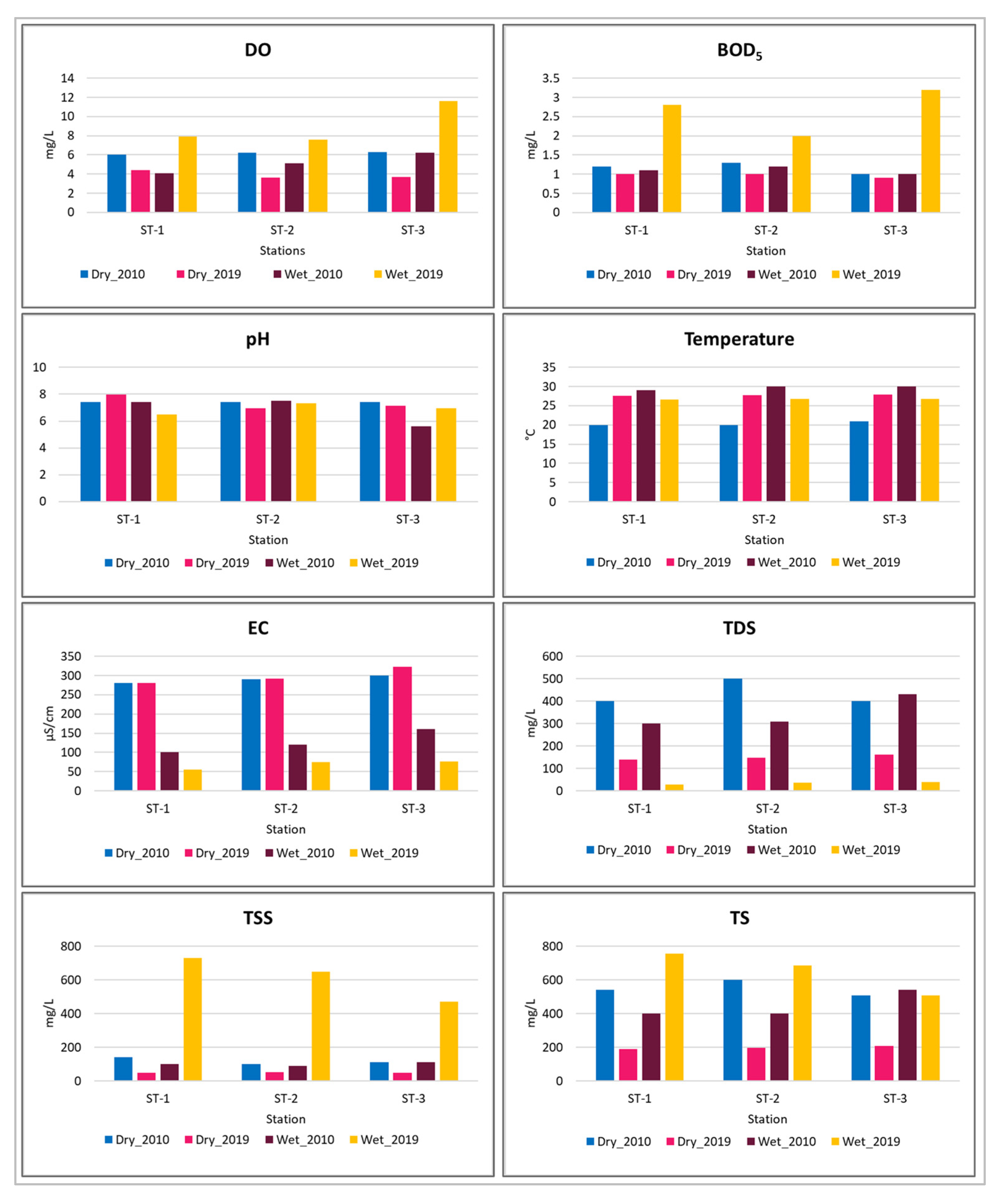
The quality of water throughout the dry and wet seasons in 2010 and 2019 are presented in Table 2 and Table 3, respectively, and in Figure 3. DO levels ranged from 3.6 mg/L to 4.4 mg/L in the dry season and 7.6 mg/L to 11.6 mg/L in the wet season in 2019. In the wet season, the highest DO was found at Kazir Bazar, while the lowest was found at Keane Bridge in dry season. The DO level increased in all stations during the wet season. In 2010, the DO level varied from 5.1 mg/L in the wet to 6.2 mg/L in the dry season. The Surma river’s mean DO level in 2019 was higher than the DO level in 2010.
For BOD5, in 2019, the recorded average concentration of BOD5 for the Surma river water was 0.97 mg/L and 2.67 mg/L in the dry and wet seasons respectively. The seasonal comparison shows that during the wet season the BOD5 level was higher than the dry season. The lowest and the highest were found at ST-3. In 2010, the average BOD5 level was 1.2 mg/L (dry season) and 1.1 mg/L (wet season). The mean BOD5 level slightly increased in 2019 as compared with 2010.
In 2019, the measured pH amongst different stations varied between 6.97 and 7.96 in the dry season, indicating almost neutral-to-slightly-alkaline water conditions. While in the wet season, pH level varied between 6.47 and 7.31. The average dry season pH was slightly alkaline, while the pH of the wet season was almost neutral. In 2010, Surma river water was almost neutral, and pH varied from 7.4 (dry season) to 6.8 (wet season). The mean value of pH was close to neutral in 2010 and 2019.
The average dry season water temperature was 20.3 °C in 2010 and 27.77 °C in 2019, while the average wet season water temperature was 29.6 °C in 2010 and 26.7 °C in 2019. Kazir Bazar had the highest dry season temperature in 2019 and Keane Bridge, as well as Kazir Bazar, had the highest wet season temperature in 2010. The recorded lowest wet season temperature was at ST-1 in the year 2010 and the lowest dry season temperature was at ST-1 and ST-2 in the year 2010. The mean temperature in 2019 is higher than the mean temperature in 2010. The temperature increased during the dry season from 2010 to 2019 but declined during the wet season. The maximum and minimum electrical conductivity (EC) of the Surma river was 322.7 µS/cm at Kazir Bazar in the dry season of 2019 and 54.46 µS/cm at Shahjalal Bridge in the wet season of 2019. During the dry season, EC was high. From 2010 to 2019, the mean EC level decreased.
The results of TDS showed that in 2019 the mean TDS concentrations were 149.47 mg/L (dry season) and 34.11 mg/L (wet season). In the dry and wet seasons, maximum TDS was found at Kazir Bazar (ST-3) and minimum TDS was found at ST-1. The mean TDS concentration in 2010 was significantly higher than the mean TDS concentration in 2019. The average maximum (616.67 mg/L) and minimum (49.9 mg/L) TSS concentrations were recorded during the wet and the dry season, respectively, in 2019. In 2019, the mean concentration of TSS was higher than the concentration of the year 2010. From 2010 to 2019, the TSS level increased, on the other hand, the TDS level decreases. In 2019, the recorded total solids (TS) in the dry season varied from 188.7 mg/L at Shahjalal Bridge (ST-1) to 209.9 mg/L at Kazir Bazar (ST-3). The TS ranged from 507.9 mg/L (minimum) at ST-3 to 757.23 mg/L (maximum) at ST-1. The seasonal comparison of the average TS level showed that the wet season’s concentration was higher than the dry season’s. In 2010, the average TSS concentration varied from 446.6 mg/L during the wet season to 550 mg/L during the dry season with a mean concentration of 498.3 mg/L that was greater than the mean concentration in 2019.
3.2. Descriptive Statistics of the Water Quality Parameters (WQPs)
The descriptive statistics of the WQPs of the Surma River from the year 2010 to 2019 are explained in Table 4.
3.3. LULC Change in the Buffer Zone
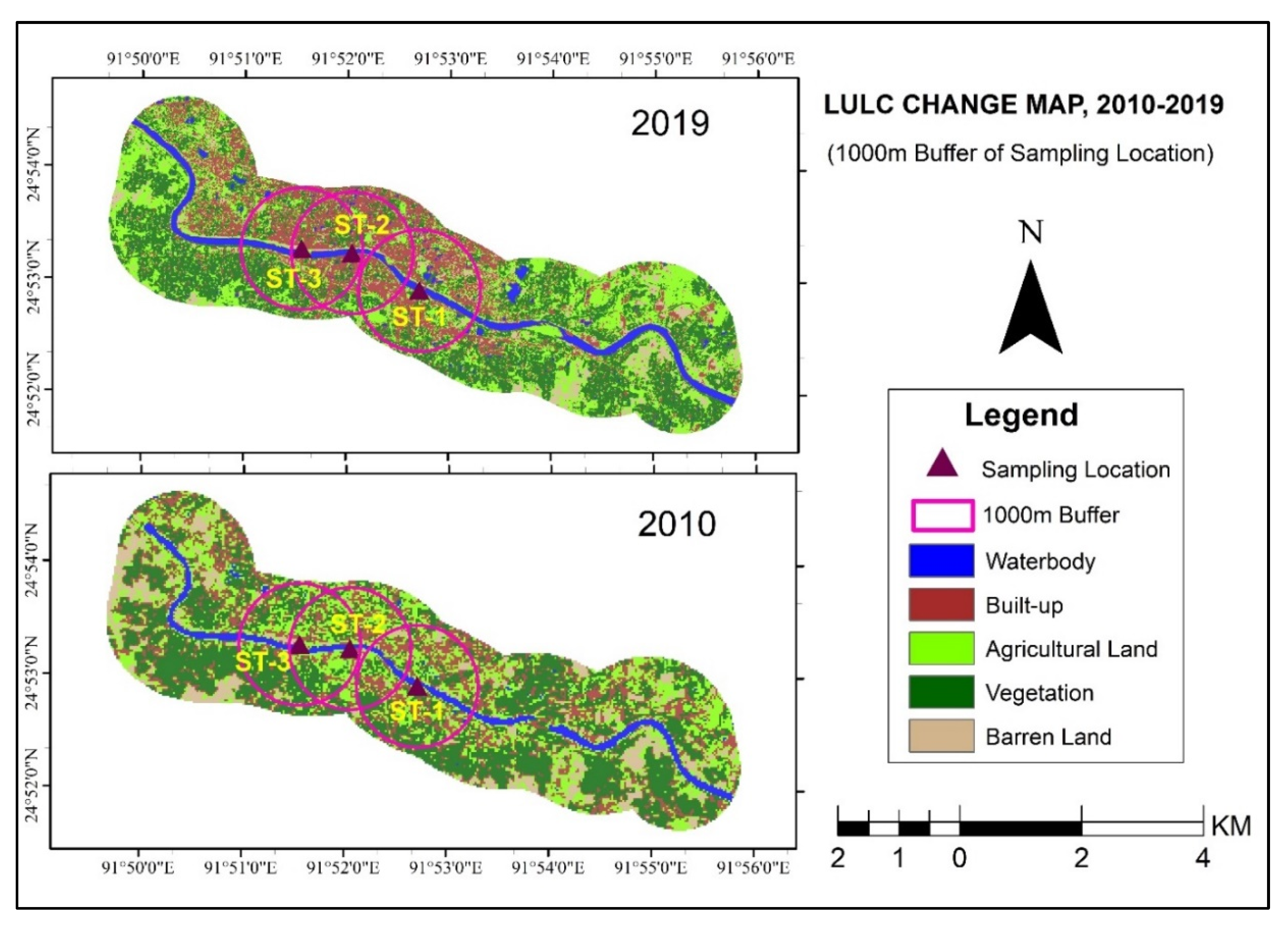
Land use change data, as the percentage of land of 1000-m buffer zone of monitoring stations, were derived from LULC change analysis from 2010 to 2019, and they were linked with water quality data. The results show that, in 2019, the central part was dominated by built-up area, while in 2010, built-up area was not clustered at a specific zone (Figure 4).
The LULC change in the buffer zones showed that the agricultural land area decreased while the built-up area significantly increased from 2010 to 2019. During this period, the increase of barren land and decrease of vegetation area was also observed in the buffer zones. In 2019 the highest built-up area was found at the buffer zone of station ST-2.
The analysis illustrated that in 2010, at ST-1 (32.4%) and ST-2 (39.9%), agricultural land usage was dominant in the 1000-m buffer zones (Table 5). On the other hand, vegetation cover (40.6%) was the dominant land area in 2010 at ST-3. In 2019, the built-up area increased in all zones and become the dominant land-use type.
By comparing land usage distribution from 2010 to 2019, all zones had shown a notable decline in agricultural land area. For the built-up area, the ST-2 zone showed a maximum increase (22.8%), while the ST-1 zone showed a minimum increase (11.7%), and at the ST-3zone, 21.1% area increased.
3.4. Descriptive Statistics of the LULC Types
The descriptive statistics of LULC types within a 1000-m buffer zone at stations of the Surma River area from 2010 to 2019 are reported in Table 6.
In 2010, waterbody ranged from 5.39% to 6.28% with a mean value of 5.84% ± 0.45%. In 2019, the range and mean of waterbody are 6.91% to 7.5% and 7.15% ± 0.31% respectively. The built-up area, from 2010 to 2019, ranged from 18.71% to 30.12% and from 38.81% to 48.57%, with a mean value of 24.89% ± 5.76% and 43.07% ± 5.00%, respectively. Agricultural land use ranged from 32.28% to 39.87% in 2010, with a mean value of 34.84% ± 4.36%. On the other hand, in 2019, agricultural land use ranged from 18.06% to 23.83% with a mean value of 20.07% ± 3.26%.
Vegetation area in 2010 and 2019 ranged from 26.72% to 40.62% and from 20.67% to 32.26% with a mean value of 31.73% ± 7.72% and 25.1% ± 6.26%, respectively. Barren land ranged from 2.17% to 3.36% in 2010, with a mean value of 2.7% ± 0.61%. On the other hand, in 2019, barren land cover ranged from a minimum of 3.58% to a maximum of 6.18% with a mean value of 4.62% ± 1.37%.
3.5. Water Quality Relation with LULC
Correlation Analysis
A correlation analysis revealed that LULC patterns were correlated significantly with one or more parameters of water quality within the 1000-m buffer zone scale (Table 7). The analysis result reveals that only BOD5, temperature, EC, TDS, and TSS had a strong and significant relationship at the 5% level of significance with the different LULC types. Other parameters viz. DO, pH, and TS had both positive and negative relationships with the LULC types but were not significant. BOD5 was found to have a positive significant relationship with waterbody (0.82), which means that, if the waterbody should increase, the BOD5 level will also increase at a significant level. At the same time, it was also found that temperature had a positive significant relationship with waterbody (0.82) but it had a negatively significant relationship with agricultural land (−0.90). This result reveals that, with the increase in agricultural land area, temperature will decrease at a significant level or vice-versa.
Electric conductivity (EC) had about a perfect positive significant relationship with vegetation (0.92) but a negative relationship with the land use types of built-up area (−0.82) and barren land (−0.84). Total dissolved solids (TDS) had also a significant relationship at the 5% level of significance, with three types of LULC types whereas total suspended solid (TSS) had four types of LULC types. Pearson’s correlation result revealed that with the increase of waterbody and built-up area TSS value will increase significantly (a positive relationship) but the TDS value will decrease significantly (a negative relationship). A different result was also found for agricultural land; agricultural land had inverse relationships with the changes in TDS and TSS. The result reveals that, if agricultural land increases, TDS (0.92) will also increase significantly at the 5% level of significance, but TSS (−0.83) will decrease.
Vegetation cover was only correlated with the change of electric conductivity, which had about a perfect positive significant correlation.
3.6. Fulfillment of Distributional Assumption of Dependent Variables
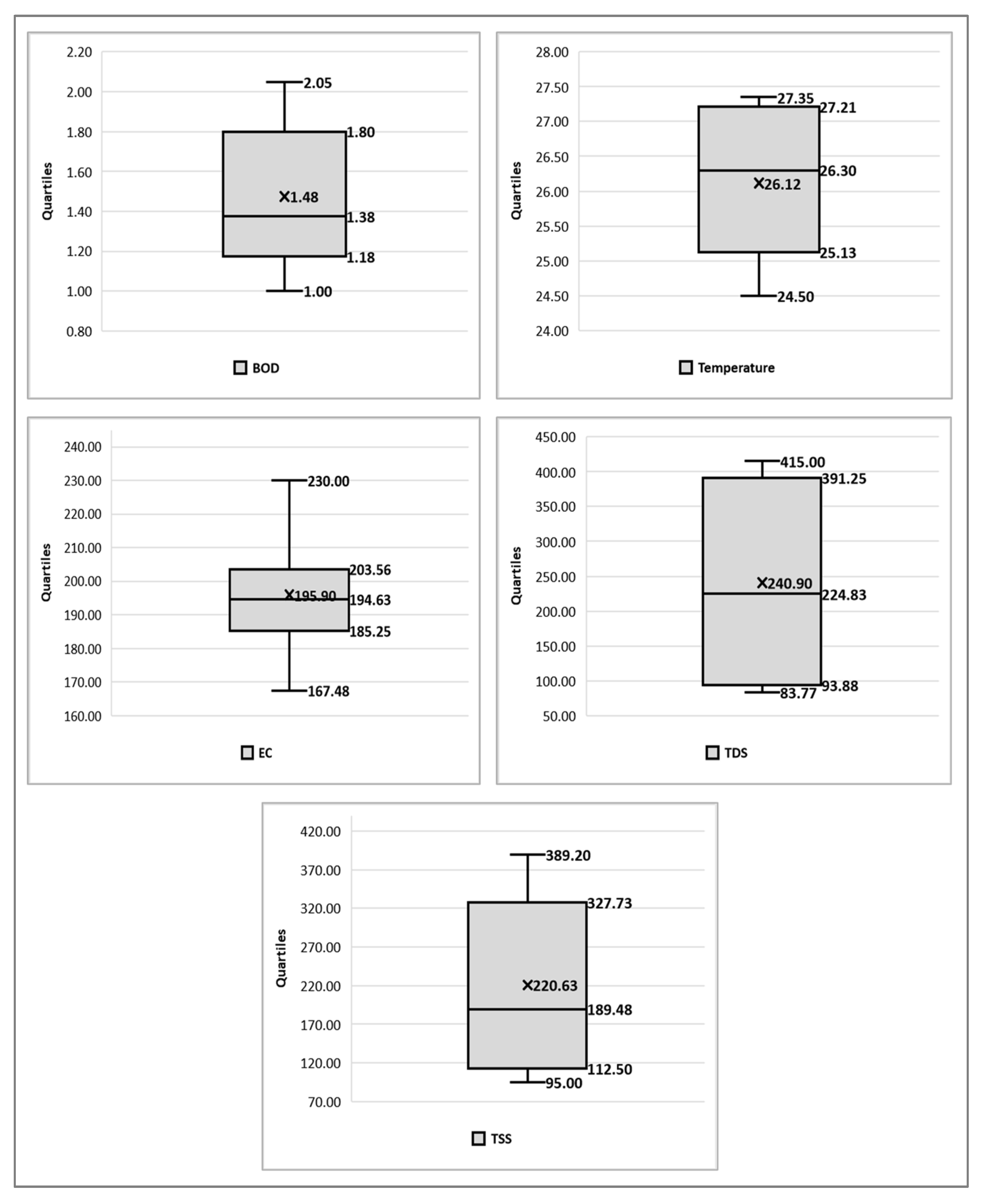
The median of BOD5 was found at 1.38, which was very similar to the average BOD5 (1.48). The similarity between mean BOD5 and median BOD5 seems to follow the symmetrical distribution of BOD5, which means that the dependent variable, BOD5, fulfills the distributional assumption for the classical model.
The similarity between the mean (26.12) and median (26.30) temperatures indicates that temperature seems to follow the normal distribution (Figure 5). There were no observed outliers in temperature, thus we can proceed to the classical model with it. The variable EC seems to follow a bell-shaped distribution, because its second quartile (194.63) lay in the middle of the first (185.25) and third (203.56) quartile. With the fulfillment of the distributional assumption of EC, we can proceed to a classical model.
The median of TDS was found as 224.83 and lay in the middle of the first quartile (93.88) and third quartile (391.25). That’s why the small departure of median TDS from mean TDS does not affect the symmetrical shape of TDS. Thus, we can proceed to a classical model for TDS.
The small departure of median TSS from the middle position of the box may have a small effect, an asymmetric shape, and also there was a difference between the mean TSS (220.63) and the median TSS (189.48). This means that TSS may follow a slightly skewed distribution. So, we can, but barely, proceed to the classical model with TSS.
3.7. Regression Analysis
Backward stepwise regression identified the relationship between WQP and LULC types that determine the combination of land uses for water quality estimation (Table 8). For the case of BOD5, only the waterbody was used as a predictor, which was found significant in a Pearson’s correlation analysis. Waterbody was not found as an especially strong predictor, as the adjusted r-squared value was 0.645. For temperature, waterbody and agricultural land were used as predictors (R2 = 0.889). Similarly, for electric conductivity, built-up, vegetation, and barren land were used as predictors (R2 = 0.833). For total dissolved solid, waterbody, built-up, and agricultural land were used as predictors (R2 = 0.993). For TSS, waterbody, built-up, and barren land were used as predictors at R2 of 0.922. From the regression analysis, it could be concluded that BOD5 showed sensitivity to changing waterbody, whereas temperature was sensitive to changing waterbody and agricultural land. EC showed sensitivity on built-up, vegetation, and barren land. TDS showed sensitivity on the waterbody, built-up and agricultural land whereas, TSS for waterbody, built-up and barren land. In this study, different parameters of water quality viz. biological oxygen demand, electric conductivity, TDS, and TSS, tended to be most affected by built-up and waterbody land usage types.
The equation for BOD5 explains, that for a one-unit change of waterbody, BOD5 would increase 0.068 times. For temperature, it would decrease, both for waterbody and agricultural land. In the same way, the equation for electric conductivity explains that, if the built-up area increases by one unit, EC will decrease 0.802 times, and for barren land, it will decrease 7.369 times. Yet, EC could increase 1.332 times if vegetation covers were increased by one unit. For TDS and TSS, the changes were the same, as is quantified and described in their equations.
4. Discussion
The water quality of any river is sturdily influenced by landscape characteristics, including land use land cover types and their spatial patterns [31]. LULC change mainly depends on how humans alter the natural landscapes and socioeconomic growth through space and time. Land covers involve the physical features of the Earth’s surface that are occupied by vegetation, water, soil, and other characteristics of the Earth’s surface created through human activities, whereas land used by human beings for habitats concerning economic activities is referred to as land cover [32].
River water qualities near the urban area changed due to several factors and LULC change was the most significant among them. LULC change has had a major impact on water quality. In the urbanization process, the built-up area increases rapidly. As a result, the quality of surrounding river water deteriorates. The rapid expansion of human settlements in the urbanized area discharge huge volumes of sewage water, as the point source of pollution, which includes a high level of nutrients and metals. Therefore, water physicochemical parameters such as pH, dissolved oxygen, biochemical oxygen demand, and chemical oxygen demand have significantly changed. The impact of land-use changes on water quality is usually studied by analyzing the relationships between land use and water quality parameters. Water quality differs according to location, time, weather, and pollution sources [33,34], and contamination is generally determined by studying the physical and chemical properties of the water bodies [35].
Findings from this study indicate that LULC types are considerably associated with one or more water quality parameters in the 1000-m buffer zone scale. It also reveals that only BOD, temperature, EC, TDS, and TSS had a strong and significant relationship with the different LULC types. In comparison, Kerala observed the water quality parameters of the Chalakudy river and compared them with diverse land use patterns over four seasons [36]. They found that urban land use was associated with poor water quality during the study period when there were changes in land use and land cover patterns [37]. Moreover, land use changes in the surrounding area of cities can modify the surface properties of watersheds that influence runoff quality and quantity. The impact of LULC changes on water quality involves analyzing the relationship between land use and water quality indicators [38]. In this research, among five types of land use and land cover, waterbody and built-up were the most significant variables in predicting water quality parameters. The Pearson correlation suggested that BOD is positively correlated with waterbody and built-up area but negatively correlated with agricultural land. A similar study by Tong and Chen [39] observed the water quality of a watershed in relation to land use change in Ohio State, USA, and their results indicate that BOD was positively correlated with residential and commercial lands but had only a non-significant correlation with agricultural land. Xiao et al. [40] conducted a multi-scale analysis of the relationship between urban river water qualities with landscape patterns in different seasons in Huzhou City, China, and their findings point out that, at a different scale, their relationships varied with the composition of land-use types—but, built-up land was most significant. These results suggest that with the development of different types of built-up land, water quality parameters change and exacerbate contamination.
Regression analysis of the present study showed that BOD was sensitive to changing waterbody, whereas temperature was sensitive to changing waterbody and agricultural land. Urban land is a mixture of different land uses types, such as residential, industrial, commercial, and other built-up areas. In contrast with other land use, wastewater is generated more in urban areas, and also urbanization increased coverage by impervious surfaces, which influences storm flow speed and runoff volumes [41]. Runoff and the huge volume of storm and drainage water are mainly responsible for this relationship between BOD and waterbody sensitivity because a higher BOD value indicates that a greater amount of organic matter is present; thus, storm flows and drainage water deliver more pollutants to the surrounding urban catchment, especially in a river. Due to the huge volume of drainage and stormwater, the pollutant quantity increased for this reason in the wet seasons, while BOD was high at a few stations.
The present study’s Pearson’s correlation results showed that, with the increase of waterbody and built-up, TSS will increase significantly (a positive relationship) and backward stepwise regression identified a relationship between WQP and LULC types, indicating that TDS were sensitive to waterbody, built-up, and agricultural land, whereas TSS was found sensitive for waterbody, built-up and barren land. Wang and Zhang [42] studied the relationship between landscape types and water quality index (WQI), in a multi-scale analysis in the Ebinur Lake oasis; their findings revealed that, for different buffers, both positive and negative relationships exist between certain land use and land cover (LULC) types and the water quality index, but there was considerable correlation between water quality index and landscape index. Li et al. [43] found a relationship between land use/cover and water quality using correlation and regression analyses in the Liao River basin, China, also indicating that BOD5, COD, sediment, and hardness were considerably associated with land use.
Although, in reviewing the literature, we found similar studies from different parts of the world, but, considering that the present work is the first such kind of investigation for a data-scarce region such as our study area, these results hold a lot of merit to both scientific communities as well as policy makers. This scientific evidence will lay a foundation for designing more robust adaptation and mitigation measures for water resource management in a timely manner.
5. Conclusions
The study revealed the concentrations of several physicochemical parameters of river water in relation to LULC changes. However, the result of the present investigation indicates that LULC changes and seasonal variations (influences the concentration) have a significant impact on water quality parameters. The results of the LULC change analysis indicate built-up, waterbody, and barren land increased and agricultural land and vegetation decreased. Built-up area is dominant in LULC types and the change of LULC pattern within 1000-m buffer zones had a significant impact on the water quality parameters of the Surma river. LULC information, in relation to the surrounding river water quality in urban areas, is very important for planning, monitoring, and management of river water because, in urbanized and densely populated cities, river water is also used for drinking purposes, after treatment, and also for recreational purposes. LULC change causes severe environmental problems worldwide and poses a threat to water quality. Spatiotemporal information about LULC change patterns with water quality helps in finding a solution to this problem. The study provides useful tools for future study, which, combined with LULC change and its relationship with different water quality parameters, can help decision-makers in formulating of rules and guidelines about sustainable land use, especially in city areas, and aid in minimizing negative impacts on water quality.
Author Contributions
Conceptualization: A.K., Z.A., M.M.U., Z.X., P.K.; methodology: A.K., Z.A.; formal analysis: A.K., Z.A.; writing—original draft preparation: A.K., Z.A., M.M.U., Z.X., P.K.; writing—review and editing: A.K., Z.A., M.M.U., Z.X., P.K.; funding acquisition: P.K. All authors have read and agreed to the published version of the manuscript.
Funding
Research work was supported by the Ministry of Science and Technology, Bangladesh, under the National Science and Technology (NST) Fellowship (FY 2018-19). Also, the publication is supported by the Asia-Pacific Network for Global Change Research (APN) under Collaborative Regional Research Programme (CRRP) with project reference number CRRP2019-01MY-Kumar.
Institutional Review Board Statement
Not applicable.
Informed Consent Statement
Not applicable.
Data Availability Statement
Not applicable.
Conflicts of Interest
The authors declare no conflict of interest.
References
- Haygarth, P.M.; Jarvis, S.C. (Eds.) Agriculture, Hydrology, and Water Quality; CABI Publishing: Wallingford, UK, 2002. [Google Scholar]
- Zhou, T.; Wu, J.; Peng, S. Assessing the effects of landscape pattern on river water quality at multiple scales: A case study of the Dongjiang River watershed, China. Ecol. Indic. 2012, 23, 166–175. [Google Scholar] [CrossRef]
- Naher, T.; Chowdhury, M.A.I. Assessment and Correlation Analysis of Water Quality Parameters: A Case Study of Surma River at Sylhet Division, Bangladesh. Int. J. Eng. Trends Technol. 2017, 53, 126–136. [Google Scholar] [CrossRef]
- UNEP-IETC. Planning and Management of Lakes and Reservoirs: An Integrated Approach to Eutrophication; UNEP-IETC: Osaka, Japan, 1997; Volume 11. [Google Scholar]
- Bhat, S.; Jacobs, J.M.; Hatfield, K.; Prenger, J. Relationships between stream water chemistry and military land use in forested watersheds in Fort Benning, Georgia. Ecol. Indic. 2006, 6, 458–466. [Google Scholar] [CrossRef]
- Hopkins, R.L. Use of landscape pattern metrics and multiscale data in aquatic species distribution models: A case study of a freshwater mussel. Landsc. Ecol. 2009, 24, 943–955. [Google Scholar] [CrossRef]
- Bhaduri, B.; Harbor, J.O.N.; Engel, B.; Grove, M. Assessing watershed-scale, long-term hydrologic impacts of land-use change using a GIS-NPS model. Environ. Manag. 2000, 26, 643–658. [Google Scholar] [CrossRef]
- Kumar, P. Numerical quantification of current status quo and future prediction of water quality in eight Asian megacities: Challenges and opportunities for sustainable water management. Environ. Monit. Assess. 2019, 191, 319. [Google Scholar] [CrossRef]
- Zhu, C. Land Use/Land Cover Change and Its Hydrological Impacts from 1984 to 2010 in the Little River Watershed, Tennessee. 2011. Available online: https://trace.tennessee.edu/cgi/viewcontent.cgi?article=2228&context=utk_gradthes (accessed on 5 February 2020).
- Hossain, M.S. Impact of land use change on stream water quality: A review of modelling approaches. J. Res. Eng. Appl. Sci. 2017, 2. [Google Scholar]
- Griffith, J.A. Geographic techniques and recent applications of remote sensing to landscape-water quality studies. Water Air Soil Pollut. 2002, 138, 181–197. [Google Scholar] [CrossRef]
- Li, K.; Chi, G.; Wang, L.; Xie, Y.; Wang, X.; Fan, Z. Identifying the critical riparian buffer zone with the strongest linkage between landscape characteristics and surface water quality. Ecol. Indic. 2018, 93, 741–752. [Google Scholar] [CrossRef]
- Goldstein, R.M.; Carlisle, D.M.; Meador, M.R.; Short, T.M. Can basin land use effects on physical characteristics of streams be determined at broad geographic scales? Environ. Monit. Assess. 2007, 130, 495–510. [Google Scholar] [CrossRef]
- Pegram, G.C.; Görgens, A.H.M. A Guide to Non-Point Source Assessment: To Support Water Quality Management of Surface Water Resources in South Africa; Water Research Commission: Cape Town, South Africa, 2001. [Google Scholar]
- Uriarte, M.; Yackulic, C.B.; Lim, Y.; Arce-Nazario, J.A. Influence of land use on water quality in a tropical landscape: A multi-scale analysis. Landsc. Ecol. 2011, 26, 1151. [Google Scholar] [CrossRef] [Green Version]
- Hassan, Z.U.; Shah, J.A.; Kanth, T.A.; Pandit, A.K. Influence of land use/land cover on the water chemistry of Wular Lake in Kashmir Himalaya (India). Ecol. Process. 2015, 4, 9. [Google Scholar] [CrossRef] [Green Version]
- McMillan, S.K.; Tuttle, A.K.; Jennings, G.D.; Gardner, A. Influence of restoration age and riparian vegetation on reach-scale nutrient retention in restored urban streams. JAWRA J. Am. Water Resour. Assoc. 2014, 50, 626–638. [Google Scholar] [CrossRef]
- Giao, N.T.; Cong, N.V.; Nhien, H.T.H. Using Remote Sensing and Multivariate Statistics in Analyzing the Relationship between Land Use Pattern and Water Quality in Tien Giang Province, Vietnam. Water 2021, 13, 1093. [Google Scholar] [CrossRef]
- Li, S.; Peng, S.; Jin, B.; Zhou, J.; Li, Y. Multi-scale relationship between land use/land cover types and water quality in different pollution source areas in Fuxian Lake Basin. PeerJ 2019, 7, e7283. [Google Scholar] [CrossRef] [PubMed] [Green Version]
- Gu, Q.; Hu, H.; Ma, L.; Sheng, L.; Yang, S.; Zhang, X.; Zhang, M.; Zheng, K.; Chen, L. Characterizing the spatial variations of the relationship between land use and surface water quality using self-organizing map approach. Ecol. Indic. 2019, 102, 633–643. [Google Scholar] [CrossRef]
- Chen, D.; Elhadj, A.; Xu, H.; Xu, X.; Qiao, Z. A Study on the Relationship between Land Use Change and Water Quality of the Mitidja Watershed in Algeria Based on GIS and RS. Sustainability 2020, 12, 3510. [Google Scholar] [CrossRef]
- Ribeiro, K.H.; Favaretto, N.; Dieckow, J.; Souza, L.C.D.P.; Minella, J.P.G.; Almeida, L.D.; Ramos, M.R. Quality of surface water related to land use: A case study in a catchment with small farms and intensive vegetable crop production in southern Brazil. Rev. De Ciência Do Solo 2014, 38, 656–668. [Google Scholar] [CrossRef] [Green Version]
- Xiao, H.; Ji, W. Relating landscape characteristics to non-point source pollution in mine waste-located watersheds using geospatial techniques. J. Environ. Manag. 2007, 82, 111–119. [Google Scholar] [CrossRef] [PubMed]
- Yang, X. An assessment of landscape characteristics affecting estuarine nitrogen loading in an urban watershed. J. Environ. Manag. 2012, 94, 50–60. [Google Scholar] [CrossRef]
- Mitchell, M.G.; Bennett, E.M.; Gonzalez, A. Linking landscape connectivity and ecosystem service provision: Current knowledge and research gaps. Ecosystems 2013, 16, 894–908. [Google Scholar] [CrossRef]
- Shen, Z.; Hou, X.; Li, W.; Aini, G.; Chen, L.; Gong, Y. Impact of landscape pattern at multiple spatial scales on water quality: A case study in a typical urbanised watershed in China. Ecol. Indic. 2015, 48, 417–427. [Google Scholar] [CrossRef]
- Chowdhury, M.H. Surma River. 2015. Available online: http://en.banglapedia.org/index.php?title=Surma_River (accessed on 3 January 2020).
- American Public Health Association (APHA). Standard Methods for the Examination of Water and Wastewater; APHA: Washington DC, USA, 2005. [Google Scholar]
- Eastman, J.R. IDRISI Taiga Guide to GIS and Image Processing; Clark Labs Clark University: Worcester, MA, USA, 2009. [Google Scholar]
- Zhang, Z.; Zhang, F.; Du, J.; Chen, D.; Zhang, W. Impacts of land use at multiple buffer scales on seasonal water quality in a reticular river network area. PLoS ONE 2021, 16, e0244606. [Google Scholar] [CrossRef] [PubMed]
- Bateni, F.; Fakheran, S.; Soffianian, A. Assessment of land cover changes & water quality changes in the Zayandehroud River Basin between 1997–2008. Environ. Monit. Assess. 2013, 185, 10511–10519. [Google Scholar]
- Rawat, J.S.; Kumar, M. Monitoring land use/cover change using remote sensing and GIS techniques: A case study of Hawalbagh block, district Almora, Uttarakhand, India. Egypt. J. Remote Sens. Space Sci. 2015, 18, 77–84. [Google Scholar] [CrossRef] [Green Version]
- Giri, S.; Qiu, Z. Understanding the relationship of land uses and water quality in twenty first century: A review. J. Environ. Manag. 2016, 173, 41–48. [Google Scholar] [CrossRef] [Green Version]
- Camara, M.; Jamil, N.R.; Abdullah, A.F.B. Impact of land uses on water quality in Malaysia: A review. Ecol. Process. 2019, 8, 10. [Google Scholar] [CrossRef]
- Duran, M.; Suicmez, M. Utilization of both benthic macroinvertebrates and physicochemical parameters for evaluating water quality of the stream Cekerek (Tokat, Turkey). J. Environ. Biol. 2007, 28, 231–236. [Google Scholar]
- Chattopadhyay, S.; Rani, L.A.; Sangeetha, P.V. Water quality variations as linked to land use pattern: A case study in Chalakudy river basin, Kerala. Curr. Sci. 2005, 89, 2163–2169. [Google Scholar]
- Chauhan, A.; Verma, S.C. Impact of Agriculture, Urban and Forest Land Use on Physico-Chemical Properties of Water-A Review. Int. J. Curr. Microbiol. Appl. Sci. 2015, 4, 18–22. [Google Scholar]
- Tu, J. Spatial and temporal relationships between water quality and land use in northern Georgia, USA. J. Integr. Environ. Sci. 2011, 8, 151–170. [Google Scholar] [CrossRef]
- Tong, S.T.; Chen, W. Modeling the relationship between land use and surface water quality. J. Environ. Manag. 2002, 66, 377–393. [Google Scholar] [CrossRef] [PubMed]
- Xiao, R.; Wang, G.; Zhang, Q.; Zhang, Z. Multi-scale analysis of relationship between landscape pattern and urban river water quality in different seasons. Sci. Rep. 2016, 6, 25250. [Google Scholar] [CrossRef] [PubMed] [Green Version]
- Waters, E.R.; Morse, J.L.; Bettez, N.D.; Groffman, P.M. Differential carbon and nitrogen controls of denitrification in riparian zones and streams along an urban to exurban gradient. J. Environ. Qual. 2014, 43, 955–963. [Google Scholar] [CrossRef] [PubMed]
- Wang, X.; Zhang, F. Multi-scale analysis of the relationship between landscape patterns and a water quality index (WQI) based on a stepwise linear regression (SLR) and geographically weighted regression (GWR) in the Ebinur Lake oasis. Environ. Sci. Pollut. Res. 2018, 25, 7033–7048. [Google Scholar] [CrossRef]
- Li, Y.L.; Liu, K.; Li, L.; Xu, Z.X. Relationship of land use/cover on water quality in the Liao River basin, China. Procedia Environ. Sci. 2012, 13, 1484–1493. [Google Scholar] [CrossRef] [Green Version]
Figure 1.
Research Design.

Figure 2.
The study area and sampling stations.

Figure 3.
Seasonal and spatial variations of WQPs in 2010 and 2019.

Figure 4.
LULC change during the period 2010–2019.

Figure 5.
Box and whisker plots of dependent variables.


Table 1.
Sampling stations with location.
| Station No. | Station Zone | Location | Flow Direction | |
|---|---|---|---|---|
| Latitude | Longitude | |||
| ST-1 | Shahjalal Bridge | 24°52′54.408″ N | 91°52′42.78″ E |  |
| ST-2 | Keane Bridge | 24°53′14.244″ N | 91°52′3.252″ E | |
| ST-3 | Kazir Bazar | 24°53′16.26″ N | 91°51′33.696″ E | |
Table 2.
Water quality during the dry and wet season in 2010.
| Parameter | DO (mg/L) | BOD5 (mg/L) | pH | Temp. (°C) | EC (μS/cm) | TDS (mg/L) | TSS (mg/L) | TS (mg/L) | |||||||||
|---|---|---|---|---|---|---|---|---|---|---|---|---|---|---|---|---|---|
| Season | Dry | Wet | Dry | Wet | Dry | Wet | Dry | Wet | Dry | Wet | Dry | Wet | Dry | Wet | Dry | Wet | |
| Station No. | ST-1 | 6 | 4.1 | 1.2 | 1.1 | 7.4 | 7.4 | 20 | 29 | 280 | 100 | 400 | 300 | 140 | 100 | 540 | 400 |
| ST-2 | 6.2 | 5.1 | 1.3 | 1.2 | 7.4 | 7.5 | 20 | 30 | 290 | 120 | 500 | 310 | 100 | 90 | 600 | 400 | |
| ST-3 | 6.3 | 6.2 | 1 | 1 | 7.4 | 5.6 | 21 | 30 | 300 | 160 | 400 | 430 | 110 | 110 | 510 | 540 | |
| Average | 6.2 | 5.1 | 1.2 | 1.1 | 7.4 | 6.8 | 20.3 | 29.6 | 290 | 126.6 | 433.3 | 346.6 | 116.6 | 100 | 550 | 446.6 | |
| Mean | 5.65 | 1.15 | 7.1 | 24.95 | 208.3 | 389.95 | 108.3 | 498.3 | |||||||||
Table 3.
Water quality during the dry and wet season in 2019.
| Parameter | DO (mg/L) | BOD5 (mg/L) | pH | Temp. (°C) | EC (μS/cm) | TDS (mg/L) | TSS (mg/L) | TS (mg/L) | |||||||||
|---|---|---|---|---|---|---|---|---|---|---|---|---|---|---|---|---|---|
| Season | Dry | Wet | Dry | Wet | Dry | Wet | Dry | Wet | Dry | Wet | Dry | Wet | Dry | Wet | Dry | Wet | |
| Station No. | ST-1 | 4.4 | 7.9 | 1 | 2.8 | 7.96 | 6.47 | 27.6 | 26.6 | 280.5 | 54.46 | 140.3 | 27.23 | 48.4 | 730 | 188.7 | 757.23 |
| ST-2 | 3.6 | 7.6 | 1 | 2 | 6.97 | 7.31 | 27.8 | 26.7 | 292.9 | 74.43 | 146.7 | 37.2 | 51.3 | 650 | 198 | 687.2 | |
| ST-3 | 3.7 | 11.6 | 0.9 | 3.2 | 7.14 | 6.94 | 27.9 | 26.8 | 322.7 | 75.81 | 161.4 | 37.91 | 47.9 | 470 | 209.3 | 507.91 | |
| Average | 3.9 | 9.03 | 0.97 | 2.67 | 7.36 | 6.91 | 27.77 | 26.7 | 298.7 | 68.23 | 149.47 | 34.11 | 49.2 | 616.67 | 198.67 | 650.78 | |
| Mean | 6.47 | 1.82 | 7.13 | 27.23 | 183.47 | 91.79 | 332.93 | 424.72 | |||||||||
Table 4.
Descriptive statistics of the WQPs.
| Water Quality Parameters | Minimum | Maximum | Mean | SD | ||||
|---|---|---|---|---|---|---|---|---|
| 2010 | 2019 | 2010 | 2019 | 2010 | 2019 | 2010 | 2019 | |
| DO (mg/L) | 5.05 | 5.60 | 6.25 | 7.65 | 5.65 | 6.47 | 0.60 | 1.06 |
| BOD5 (mg/L) | 1.00 | 1.50 | 1.25 | 2.05 | 1.13 | 1.82 | 0.13 | 0.28 |
| pH | 6.50 | 7.04 | 7.45 | 7.22 | 7.12 | 7.13 | 0.53 | 0.09 |
| temperature (°C) | 24.50 | 27.10 | 25.50 | 27.35 | 25.00 | 27.23 | 0.50 | 0.13 |
| EC (µS/cm) | 190.00 | 167.48 | 230.00 | 199.26 | 208.33 | 183.47 | 20.21 | 15.89 |
| TDS (mg/L) | 350.00 | 83.77 | 415.00 | 99.66 | 390.00 | 91.79 | 35.00 | 7.95 |
| TSS (mg/L) | 95.00 | 258.95 | 120.00 | 389.20 | 108.33 | 332.93 | 12.58 | 66.91 |
| TS (mg/L) | 470.00 | 358.61 | 525.00 | 472.97 | 498.33 | 424.72 | 27.54 | 59.24 |
Table 5.
LULC change within the 1000-m buffer zone of sampling stations.
| LULC Type | Sampling Station | |||||
|---|---|---|---|---|---|---|
| ST-1 | ST-2 | ST-3 | ||||
| 2010 (%) | 2019 (%) | 2010 (%) | 2019 (%) | 2010 (%) | 2019 (%) | |
| Waterbody | 6.3 | 7.5 | 5.4 | 6.9 | 5.8 | 7.1 |
| Built-up | 30.1 | 41.8 | 25.8 | 48.6 | 18.7 | 38.8 |
| Agricultural Land | 32.4 | 23.8 | 39.9 | 18.1 | 32.3 | 18.3 |
| Vegetation | 27.8 | 20.7 | 26.7 | 22.3 | 40.6 | 32.2 |
| Barren Land | 3.4 | 6.2 | 2.2 | 4.1 | 2.6 | 3.6 |
Table 6.
Descriptive statistics of the LULC types.
| LULC (in %) | Minimum | Maximum | Mean | SD | ||||
|---|---|---|---|---|---|---|---|---|
| 2010 | 2019 | 2010 | 2019 | 2010 | 2019 | 2010 | 2019 | |
| waterbody | 5.39 | 6.91 | 6.28 | 7.50 | 5.84 | 7.15 | 0.45 | 0.31 |
| built-up | 18.71 | 38.81 | 30.12 | 48.57 | 24.89 | 43.07 | 5.76 | 5.00 |
| agricultural land | 32.28 | 18.06 | 39.87 | 23.83 | 34.84 | 20.07 | 4.36 | 3.26 |
| vegetation | 26.72 | 20.67 | 40.62 | 32.26 | 31.73 | 25.10 | 7.72 | 6.26 |
| barren land | 2.17 | 3.58 | 3.36 | 6.18 | 2.70 | 4.62 | 0.61 | 1.37 |
Table 7.
Linear relationship (Pearson correlation, r) between WQPs and LULC types.
| LULC Types | Waterbody | Built-Up | Agricultural Land | Vegetation | Barren Land | |
|---|---|---|---|---|---|---|
| WQPs | ||||||
| DO (mg/L) | 0.38 | 0.12 | −0.50 | 0.36 | 0.09 | |
| BOD5 (mg/L) | 0.82 | 0.72 | −0.74 | −0.42 | 0.66 | |
| pH | 0.03 | 0.34 | 0.18 | −0.76 | 0.15 | |
| temperature (°C) | 0.82 | 0.79 | −0.90 | −0.32 | 0.63 | |
| EC (µS/cm) | −0.74 | −0.82 | 0.47 | 0.92 | −0.84 | |
| TDS (mg/L) | −0.94 | −0.93 | 0.92 | 0.56 | −0.79 | |
| TSS (mg/L) | 0.92 | 0.90 | −0.83 | −0.64 | 0.89 | |
| TS (mg/L) | −0.61 | −0.63 | 0.75 | 0.16 | −0.25 | |
NB: Bold letters indicates a significant relationship at the 5% level.
Table 8.
Linear regression models of LULC types on the WQPs.
| Dependent Variable (WQPs) | Independent Variables (Land Usage Type) | Estimated Linear Regression Equations | Adjusted R2 |
|---|---|---|---|
| BOD5 | Waterbody | BOD5 = 0.737 + 0.594 × Y_2019 + 0.068 × W | 0.645 |
| temperature | waterbody, agricultural land | Temp = 29.097 + 2.567 × Y_2019 − 0.546 × W − 0.026 × A | 0.889 |
| EC | built-up, vegetation, barren land | EC = 205.887 + 12.714 × Y_2019 − 0.802 × Bu + 1.332 × V − 7.369 × Ba | 0.833 |
| TDS | waterbody, built-up, agricultural land | TDS = 726.425 − 184.029 × Y_2019 − 45.117 × W − 2.988 × Bu + 0.039 × A | 0.993 |
| TSS | waterbody, built-up, barren land | TSS = 309.915 + 172.824 × Y_2019 − 68.363 × W + 1.890 × Bu + 55.799 × Ba | 0.922 |
Y_2019 = year 2019 (dummy or indicator); Temp = temperature; W = waterbody, A = agricultural land; Bu = built-up; V = vegetation; Ba = barren land.
Publisher’s Note: MDPI stays neutral with regard to jurisdictional claims in published maps and institutional affiliations. |
© 2021 by the authors. Licensee MDPI, Basel, Switzerland. This article is an open access article distributed under the terms and conditions of the Creative Commons Attribution (CC BY) license (https://creativecommons.org/licenses/by/4.0/).
Share and Cite
MDPI and ACS Style
Kadir, A.; Ahmed, Z.; Uddin, M.M.; Xie, Z.; Kumar, P. Integrated Approach to Quantify the Impact of Land Use and Land Cover Changes on Water Quality of Surma River, Sylhet, Bangladesh. Water 2022, 14, 17. https://doi.org/10.3390/w14010017
AMA Style
Kadir A, Ahmed Z, Uddin MM, Xie Z, Kumar P. Integrated Approach to Quantify the Impact of Land Use and Land Cover Changes on Water Quality of Surma River, Sylhet, Bangladesh. Water. 2022; 14(1):17. https://doi.org/10.3390/w14010017
Chicago/Turabian StyleKadir, Abdul, Zia Ahmed, Md. Misbah Uddin, Zhixiao Xie, and Pankaj Kumar. 2022. "Integrated Approach to Quantify the Impact of Land Use and Land Cover Changes on Water Quality of Surma River, Sylhet, Bangladesh" Water 14, no. 1: 17. https://doi.org/10.3390/w14010017
Note that from the first issue of 2016, this journal uses article numbers instead of page numbers. See further details here.