
Using the Change Point Model (CPM) Framework to Identify Windows for Water Resource Management Action in the Lower Colorado River Basin of Texas, USA


Abstract
:1. Introduction
2. Materials and Methods
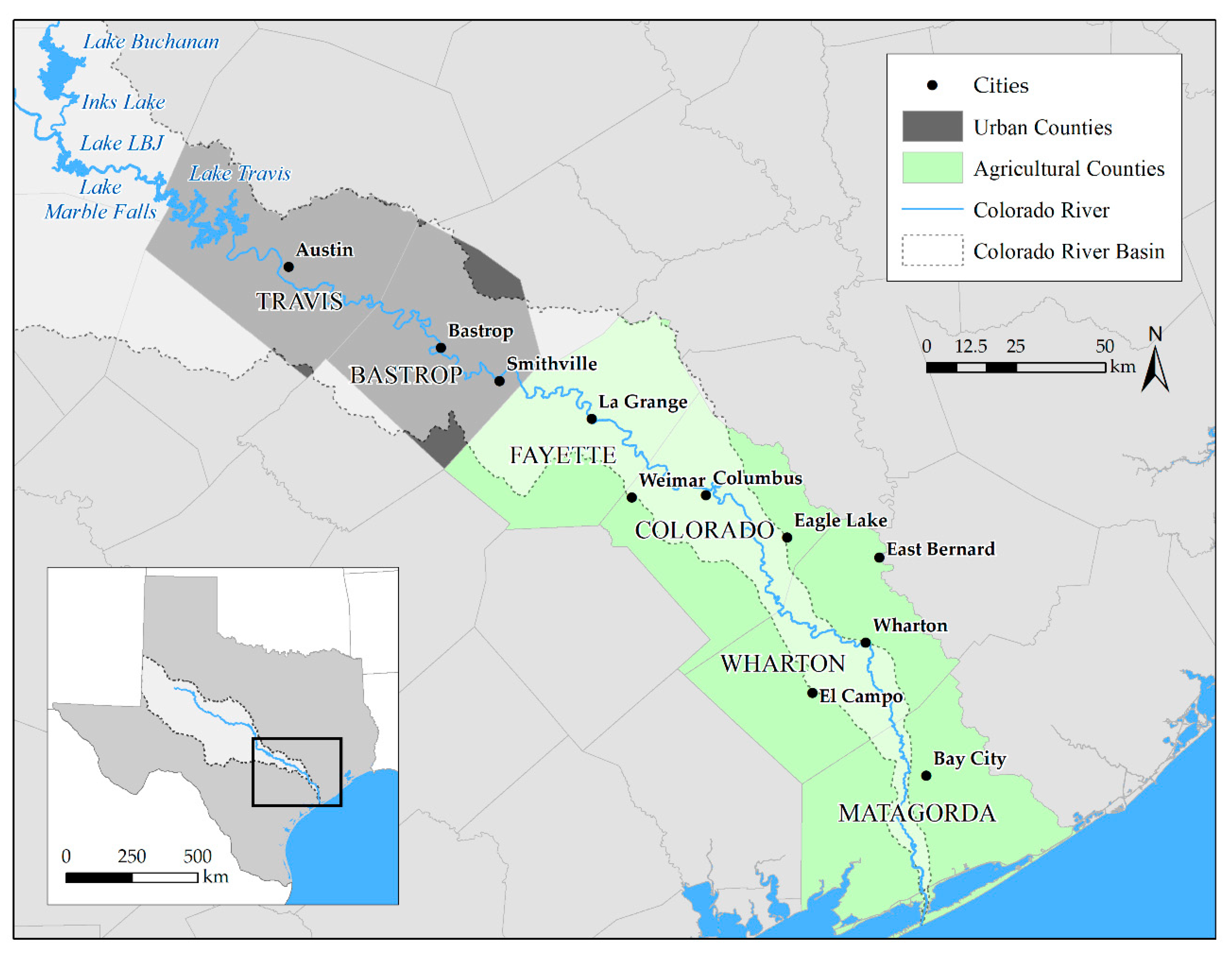
2.1. Site and Situation
2.2. Data
2.2.1. Climate-Related Indicators
2.2.2. Lake and River Characteristics
2.2.3. Water Usage Information
2.2.4. Agricultural Characteristics
2.3. Analysis
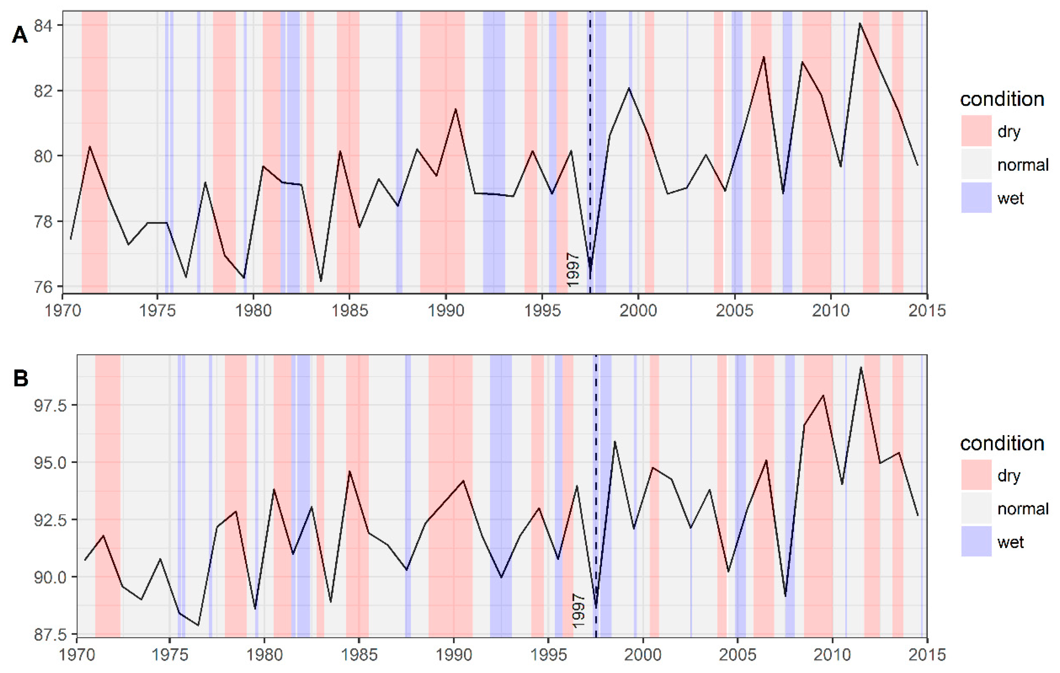
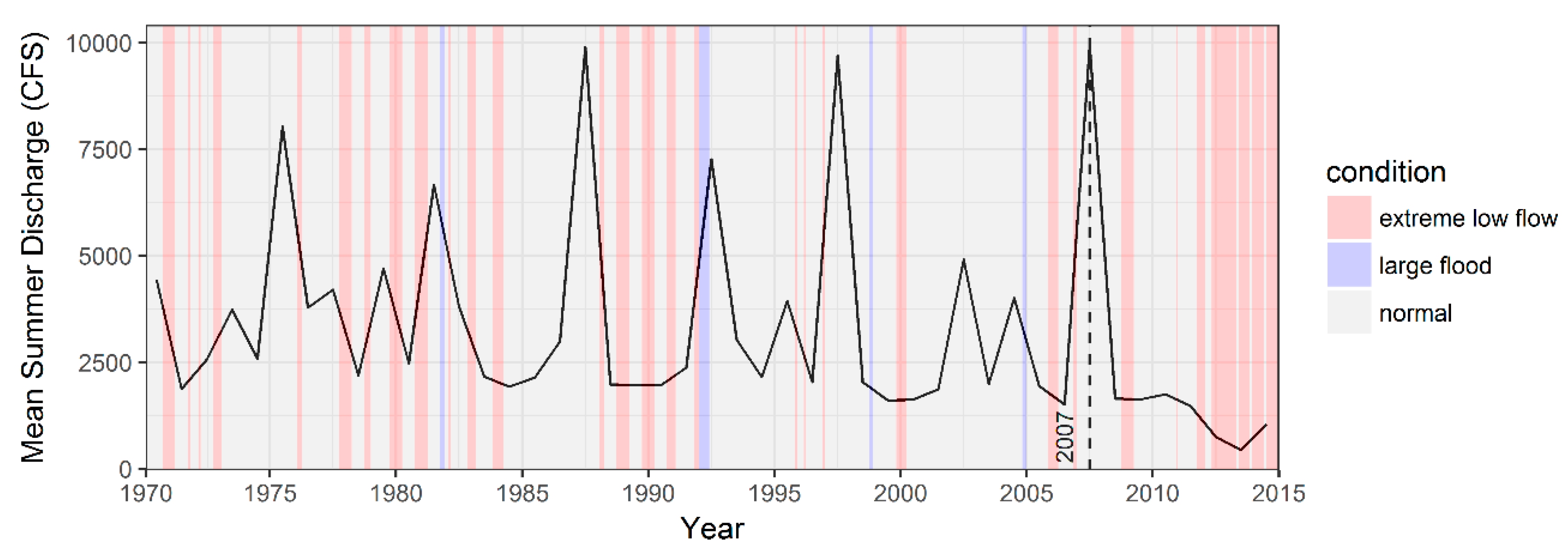
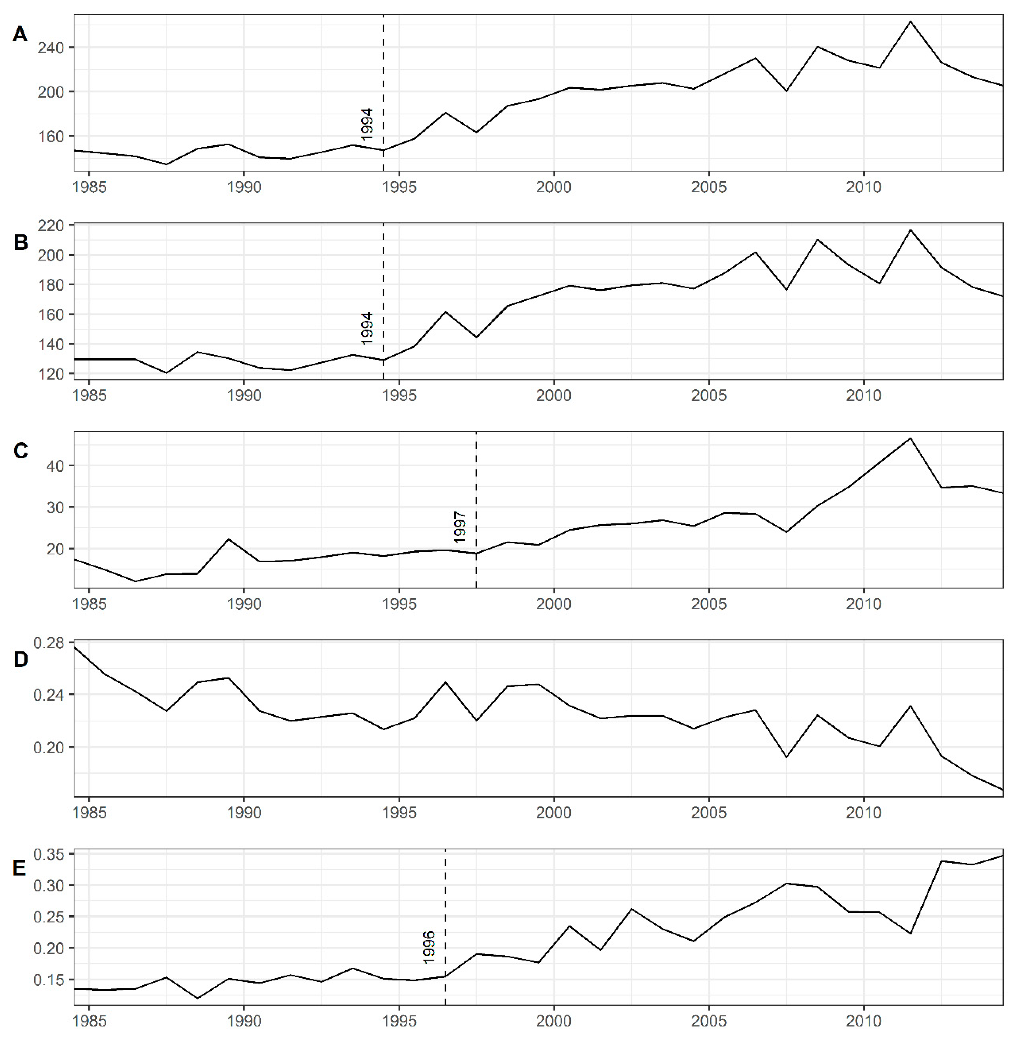
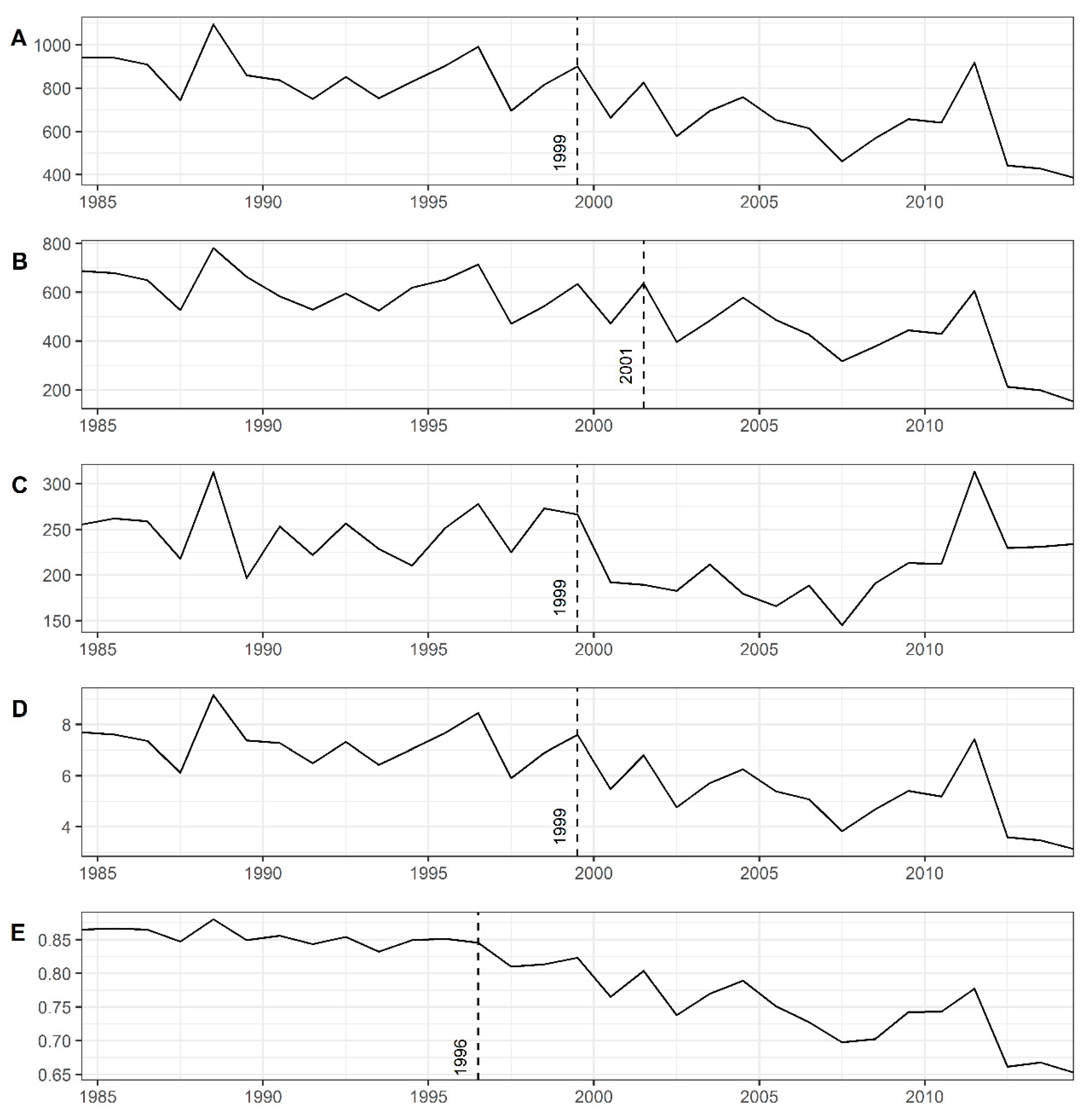
3. Results
4. Discussion
4.1. Droughts
4.2. Managerial Interventions
5. Conclusions
Author Contributions
Funding
Conflicts of Interest
References
- Molle, F.; Wester, P.; Hirsch, P. River basin development and management. In Water for Food—Water for Life: A Comprehensive Assessment of Water Managemen in Agrculture; Molden, D., Ed.; Earthscan: London, UK, 2007. [Google Scholar]
- Hellegers, P.; Leflaive, X. Water allocation reform: What makes it so difficult? Water Int. 2015, 40, 273–285. [Google Scholar] [CrossRef]
- OECD. Water Resources Allocation: Sharing Risks and Opportunities; OECD Publishing: Paris, France, 2015. [Google Scholar]
- Molle, F.; Berkoff, J. Cities vs. agriculture: A review of intersectoral water re-allocation. Nat. Resour. Forum 2009, 33, 6–18. [Google Scholar] [CrossRef]
- Howe, C.W. Water markets in Colorado: Past performance and needed changes. In Markets for Water: Potential and Performance; Easter, K.W., Rosegrant, M.W., Dinar, A., Eds.; Kluwer Academic Publishers: Boston, MA, USA, 1998. [Google Scholar]
- Celio, M.; Giordano, M. Agriculture–urban water transfers: A case study of Hyderabad, South-India. Paddy Water Environ. 2007, 5, 229–237. [Google Scholar] [CrossRef]
- Celio, M.; Scott, C.A.; Giordano, M. Urban–agricultural water appropriation: The Hyderabad, India case. Geogr. J. 2010, 176, 39–57. [Google Scholar] [CrossRef]
- Birkenholtz, T. Dispossessing irrigators: Water grabbing, supply-side growth and farmer resistance in India. Geoforum 2016, 69, 94–105. [Google Scholar] [CrossRef]
- Gleick, P.H. Transitions to freshwater sustainability. Proc. Natl. Acad. Sci. USA 2018, 115, 8863–8871. [Google Scholar] [CrossRef] [Green Version]
- Oki, T.; Kanae, S. Global hydrological cycles and world water resources. Science 2006, 313, 1068–1072. [Google Scholar] [CrossRef] [Green Version]
- Vörösmarty, C.J.; Green, P.; Salisbury, J.; Lammers, R.B. Global water resources: Vulnerability from climate change and population growth. Science 2000, 289, 284–288. [Google Scholar] [CrossRef] [Green Version]
- Mekonnen, M.M.; Hoekstra, A.Y. Four billion people facing severe water scarcity. Sci. Adv. 2016, 2, e1500323. [Google Scholar] [CrossRef] [Green Version]
- Dziegielewski, B.; Kiefer, J.C. U.S. Water Demand, Supply and Allocation: Trends and Outlook; 2007-R-3; Institute for Water Resources: Alexandria, VA, USA, 2007. [Google Scholar]
- Swyngedouw, E. Power, nature, and the city. The conquest of water and the political ecology of urbanization in Guayaquil, Ecuador: 1880–1990. Environ. Plan. A 1997, 29, 311–332. [Google Scholar] [CrossRef]
- Swyngedouw, E. Social Power and the Urbanization of Water: Flows of Power; Oxford University Press: New York, NY, USA, 2004. [Google Scholar]
- Bakker, K. Archipelagos and networks: Urbanization and water privatization in the South. Geogr. J. 2003, 169, 328–341. [Google Scholar] [CrossRef]
- Scott, C.A.; Pablos, N.P. Innovating resource regimes: Water, wastewater, and the institutional dynamics of urban hydraulic reach in northwest Mexico. Geoforum 2011, 42, 439–450. [Google Scholar] [CrossRef]
- Kaika, M. City of Flows: Modernity, Nature, and the City; Routledge: New York, NY, USA, 2005. [Google Scholar]
- Bell, M.G. Historical Political Ecology of Water: Access to Municipal Drinking Water in Colonial Lima, Peru (1578–1700). Prof. Geogr. 2015, 67, 504–526. [Google Scholar] [CrossRef]
- Wagner, K. Status and Trends of Irrigated Agriculture in Texas; TWRI EM-115; Texas Water Resources Institute: College Station, TX, USA, 2012. [Google Scholar]
- Shupe, S.J.; Weatherford, G.D.; Checchio, E. Western water rights: The era of reallocation. Nat. Resour. J. 1989, 29, 413. [Google Scholar]
- Villarejo, D. 93640 at Risk: Farmers, Workers, and Townspeople in An Era of Water Uncertainty; The California Institute for Rural Studies: Davis, CA, USA, 1996. [Google Scholar]
- Molle, F.; Hoogesteger, J.; Mamanpoush, A. Macro-and micro-level impacts of droughts: The case of the Zayandeh Rud river basin, Iran. Irrigigation Drain. 2008, 57, 219. [Google Scholar] [CrossRef]
- Chang, C.; Griffin, R.C. Water marketing as a reallocative institution in Texas. Water Resour. Res. 1992, 28, 879–890. [Google Scholar] [CrossRef]
- Debaere, P.; Li, T. The effects of water markets: Evidence from the Rio Grande. Adv. Water Resour. 2020, 145, 103700. [Google Scholar] [CrossRef]
- Molle, F. Development Trajectories of River Basins: A Conceptual Framework; International Water Management Institute: Colombo, Sri Lanka, 2003. [Google Scholar]
- Platt, R.H. Land Use and Society: Geography, Law, and Public Policy, 3rd ed.; Island Press: Washington, DC, USA, 2014. [Google Scholar]
- Lykou, R.; Tsaklidis, G.; Papadimitriou, E. Change point analysis on the Corinth Gulf (Greece) seismicity. Phys. A Stat. Mech. Appl. 2020, 541, 123630. [Google Scholar] [CrossRef]
- Barboza, L.A.; Vásquez, P.; Mery, G.; Sanchez, F.; García, Y.E.; Calvo, J.G.; Rivas, T.; Pérez, M.D.; Salas, D. The Role of Mobility and Sanitary Measures on the Delay of Community Transmission of COVID-19 in Costa Rica. Epidemiologia 2021, 2, 22. [Google Scholar] [CrossRef]
- Hallema, D.W.; Sun, G.; Caldwell, P.V.; Norman, S.P.; Cohen, E.C.; Liu, Y.; Bladon, K.D.; McNulty, S.G. Burned forests impact water supplies. Nat. Commun. 2018, 9, 1307. [Google Scholar] [CrossRef] [Green Version]
- Adams, J.A. Damming the Colorado: The Rise of the Lower Colorado River Authority 1933–1939; Texas A&M University Press: College Station, TX, USA, 1990. [Google Scholar]
- Woodruff, C.M. Land Resource Overview of the Capital Area Planning Council Region, Texas—A Nontechnical Guide; Bureau of Economic Geology: Austin, TX, USA, 1979. [Google Scholar]
- Barlow, M.; Nigam, S.; Berbery, E.H. ENSO, Pacific decadal variability, and US summertime precipitation, drought, and stream flow. J. Clim. 2001, 14, 2105–2128. [Google Scholar] [CrossRef] [Green Version]
- Combs, S. The Impact of the 2011 Drought and Beyond; Texas Comptroller: Austin, TX, USA, 2012. [Google Scholar]
- Sansom, A. Water in Texas: An Introduction; University of Texas Press: Austin, TX, USA, 2008. [Google Scholar]
- Coff, R.; Darling, K. Travis County Trend Profile: Selected Census Data from 1990, 2000, and 2010; Travis County Health and Human Services & Veterans Service, Research & Planning Division: Travis County, TX, USA, 2012; pp. 1–4. [Google Scholar]
- Baldwin, K.; Dohlman, E.; Childs, N.; Foreman, L. Consolidation and Structural Change in the US Rice Sector; RCS-11d-01; Economic Research Service/USDA: Washington, DC, USA, 2011. [Google Scholar]
- Banks, J.H.J.; Babcock, J.E. Corralling the Colorado: The First Fifity Years of the Lower Colorado River Authority; Eakin Press: Austin, TX, USA, 1988. [Google Scholar]
- Lavy, B.L. Cooperation, fragmentation and control: News media representations of changing water access from Austin to the Texas Rice Belt. Water Altern. 2020, 13, 779–799. [Google Scholar]
- LCRA. About LCRA. Available online: http://www.lcra.org/about/Pages/default.aspx (accessed on 5 September 2017).
- Kelly, M.E. Water for the environment: Updating Texas water law. In Water Policy in Texas: Responding to the Rise of Scarcity; Griffin, R.C., Ed.; RFF Press: Washington, DC, USA, 2011. [Google Scholar]
- TWDB. Water for Texas: State Water Plan; Texas Water Development Board: Austin, TX, USA, 2017. [Google Scholar]
- Franczyk, J.; Chang, H. Spatial Analysis of Water Use in Oregon, USA, 1985–2005. Water Resour. Manag. 2009, 23, 755–774. [Google Scholar] [CrossRef]
- Kaika, M. Constructing scarcity and sensationalising water politics: 170 days that shook Athens. Antipode 2003, 35, 919–954. [Google Scholar] [CrossRef]
- Bakker, K. Privatizing Water, Producing Scarcity: The Yorkshire Drought of 1995. Econ. Geogr. 2000, 76, 4–27. [Google Scholar] [CrossRef]
- Linton, J.; Budds, J. The hydrosocial cycle: Defining and mobilizing a relational-dialectical approach to water. Geoforum 2014, 57, 170–180. [Google Scholar] [CrossRef]
- Cech, T.V. Principles of Water Resources: History, Development, and Management, 3rd ed.; John Wiley & Sons, Inc.: Hoboken, NJ, USA, 2010. [Google Scholar]
- McKee, T.B.; Doesken, N.J.; Kleist, J. The relationship of drought frequency and duration to time scales. In Proceedings of the 8th Conference on Applied Climatology, Anaheim, CA, USA, 17–22 January 1993; pp. 179–183. [Google Scholar]
- McKee, T.B.; Doesken, N.J.; Kleist, J. Drought monitoring with multiple time scales. In Proceedings of the 9th Conference on Applied Climatology, Dallas, TX, USA, 15–20 January 1995; pp. 233–236. [Google Scholar]
- Agnew, C. Using the SPI to identify drought. Drought Netw. News 2000, 12, 6–12. [Google Scholar]
- WMO. Standardized Precipitation Index User Guide; World Meteorological Organization: Geneva, Switzerland, 2012. [Google Scholar]
- Hayes, M.J.; Svoboda, M.D.; Wilhite, D.A.; Vanyarkho, O.V. Monitoring the 1996 drought using the standardized precipitation index. Bull. Am. Meteorol. Soc. 1999, 80, 429–438. [Google Scholar] [CrossRef] [Green Version]
- The Nature Conservancy. Indicators of Hydrologic Alteration (IHA), version 7.1; The Nature Conservancy: Arlington County, VA, USA, 2009. [Google Scholar]
- The Nature Conservancy. Indicators of Hydrologic Alteration Version 7.1 User’s Manual; The Nature Conservancy: Arlington County, VA, USA, 2009. [Google Scholar]
- Richter, B.D.; Baumgartner, J.V.; Powell, J.; Braun, D.P. A method for assessing hydrologic alteration within ecosystems. Conserv. Biol. 1996, 10, 1163–1174. [Google Scholar] [CrossRef] [Green Version]
- Mathews, R.; Richter, B.D. Application of the indicators of hydrologic alteration software in environmental flow setting. JAWRA J. Am. Water Resour. Assoc. 2007, 43, 1400–1413. [Google Scholar] [CrossRef]
- OECD. OECD Environmental Outlook to 2050; OECD Publishing: Paris, France, 2012. [Google Scholar]
- Ross, G.J. Parametric and Nonparametric Sequential Change Detection in R: The CPM Package. J. Stat. Softw. 2015, 66, 1–20. [Google Scholar] [CrossRef] [Green Version]
- Team, R.C. R: A Language and Environment for Statistical Computing, version 3.3.2; R Foundation for Statistical Computing: Vienna, Austria, 2016. [Google Scholar]
- Beaulieu, C.; Chen, J.; Sarmiento, J.L. Change-point analysis as a tool to detect abrupt climate variations. Philos. Trans. R. Soc. A Math. Phys. Eng. Sci. 2012, 370, 1228–1249. [Google Scholar] [CrossRef] [PubMed] [Green Version]
- Thomson, J.R.; Kimmerer, W.J.; Brown, L.R.; Newman, K.B.; Nally, R.M.; Bennett, W.A.; Feyrer, F.; Fleishman, E. Bayesian change point analysis of abundance trends for pelagic fishes in the upper San Francisco Estuary. Ecol. Appl. 2010, 20, 1431–1448. [Google Scholar] [CrossRef] [Green Version]
- Obisesan, K.; Lawal, M.; Bamiduro, T.; Adelakun, A. Data Visualization and Change-point detection in Environmental Data: The Case of Water Pollution in Oyo State Nigeria. J. Sci. Res. 2013, 12, 179–188. [Google Scholar]
- Hawkins, D.M.; Qiu, P.; Kang, C.W. The Changepoint Model for Statistical Process Control. J. Qual. Technol. 2003, 35, 355–366. [Google Scholar] [CrossRef]
- Hawkins, D.M.; Zamba, K.D. Statistical Process Control for Shifts in Mean or Variance Using a Changepoint Formulation. J. Qual. Technol. 2005, 37, 21–31. [Google Scholar] [CrossRef]
- Ross, G.J.; Adams, N.M. Two nonparametric control charts for detecting arbitrary distribution changes. J. Qual. Technol. 2012, 44, 102. [Google Scholar] [CrossRef]
- WGA. 1996: Drought Response Action Plan; Western Governors’ Association: Denver, CO, USA, 1996; p. 12. [Google Scholar]
- Rogers, E.W.; Clancy, L. State water planning: Its history and its challenges. In Proceedings of the 2014 Texas City Attorneys Association Summer Conference, South Padre Island, TX, USA, 18–20 June 2014. [Google Scholar]
- TWDB. Regional Water Planning in Texas; Texas Water Development Board: Austin, TX, USA, 2016. [Google Scholar]
- Kaiser, R. Texas water law and organizations. In Water Policy in Texas: Responding to the Rise of Scarcity; Griffin, R.C., Ed.; RFF Press: Washington, DC, USA, 2011. [Google Scholar]
- LCRA and the City of Austin. First Amendment to December 10, 1987 Comprehensive Water Settlement Agreement between City of Austin and Lower Colorado River Authority; Lower Colorado River Authority: Austin, TX, USA, 1999. [Google Scholar]
- Kenney, D.S.; Klein, R.A.; Clark, M.P. Use and Effectiveness of Municipal Water Restrictions during Drought in Colorado 1. JAWRA J. Am. Water Resour. Assoc. 2004, 40, 77–87. [Google Scholar] [CrossRef]
- Mini, C.; Hogue, T.; Pincetl, S. The effectiveness of water conservation measures on summer residential water use in Los Angeles, California. Resour. Conserv. Recycl. 2015, 94, 136–145. [Google Scholar] [CrossRef]
- Texas Water Code 35.001. 2001. Available online: https://statutes.capitol.texas.gov/docs/wa/htm/wa.35.htm (accessed on 5 September 2017).
- LCRA and the City of Austin. Supplemental Water Supply Agreement by and between the City of Austin and the Lower Colorado River Authority; Lower Colorado River Authority: Austin, TX, USA, 2007. [Google Scholar]
- AARO. Drowning in the Central Texas Drought; Austin Area Research Organization: Austin, TX, USA, 2015; p. 11. [Google Scholar]
- LCRA. Lakes Buchanan and Travis Water Management Plan. and Drought Contingency Plans; Lower Colorado River Authority: Austin, TX, USA, 2015. [Google Scholar]


| Conceptual Variables | Operational Variables | Units |
|---|---|---|
| Climate-related indicators | Annual mean maximum temperature | degrees Fahrenheit |
| Summer mean maximum temperature | degrees Fahrenheit | |
| Lake and river characteristics | Lake Buchanan (annual mean sea level) | feet (ft; 0.30 m) |
| Lake Buchanan (summer mean sea level) | feet | |
| Lake Travis (annual mean sea level) | feet | |
| Lake Travis (summer mean sea level) | feet | |
| Mean summer river discharge | cubic feet per second (CFS; 0.028 m3 s−1)) | |
| Water usage | Urban counties water use | thousands of acre-feet per year (AFY; 1.23 × 10⁶ m3 year−1) |
| information | Surface water use | thousands AFY |
| Groundwater use | thousands AFY | |
| Water use per capita | thousands AFY | |
| Water share | proportion | |
| Agricultural counties water use | thousands of AFY | |
| Surface water use | thousands of AFY | |
| Groundwater use | thousands of AFY | |
| Water use per capita | thousands of AFY | |
| Water share | proportion | |
| Agricultural characteristics | Total field crops harvested | thousands of acres (ac; 0.405 ha) |
| Rice harvested | thousands of acres | |
| Rice produced | thousands of hundredweight (cwt; 4.54 × 10⁴ kg) | |
| Rice share of harvest | proportion |
| Period of Change | Time Series Variable | Change Point (Year) | Documented Managerial Event (Year) |
|---|---|---|---|
| Period 1 (1994 to 1997) | Urban counties’ water use | 1994 | Senate Bill 1 (1997) |
| Urban counties’ surface water use | 1994 | House Bill 1437 (1999) | |
| Rice share of harvest | 1995 | Water Rights Purchases (1998, 1999) | |
| Urban counties’ water share | 1996 | Austin-LCRA Water Deal (1999) | |
| Rice produced | 1996 | ||
| Annual mean maximum temperature | 1997 | ||
| Summer mean maximum temperature | 1997 | ||
| Urban counties’ groundwater use | 1997 | ||
| Period 2 (1999 to 2002) | Agricultural counties’ water use | 1999 | Senate Bill 2 (2001) |
| Agricultural groundwater use | 1999 | Water Rights Purchase (2001) | |
| Agricultural water use per capita | 1999 | ||
| Rice harvested | 1999 | ||
| Agricultural counties’ surface water use | 2001 | ||
| Total field crops harvested | 2002 | ||
| Period 3 (2005 to 2007) | Lake Buchanan (annual mean sea level) | 2005 | Senate Bill 3 (2007) |
| Lake Buchanan (summer mean sea level) | 2005 | Proposition 3 (2013) | |
| Lake Travis (annual mean sea level) | 2005 | Austin-LCRA Water Deal (2007) | |
| Lake Travis (summer mean sea level) | 2007 | Water Curtailment (2011–2015) | |
| Mean summer river discharge | 2007 | Water Management Plan (2015) |
Publisher’s Note: MDPI stays neutral with regard to jurisdictional claims in published maps and institutional affiliations. |
© 2021 by the authors. Licensee MDPI, Basel, Switzerland. This article is an open access article distributed under the terms and conditions of the Creative Commons Attribution (CC BY) license (https://creativecommons.org/licenses/by/4.0/).
Share and Cite
Lavy, B.L.; Weaver, R.C.; Hagelman, R.R., III. Using the Change Point Model (CPM) Framework to Identify Windows for Water Resource Management Action in the Lower Colorado River Basin of Texas, USA. Water 2022, 14, 18. https://doi.org/10.3390/w14010018
Lavy BL, Weaver RC, Hagelman RR III. Using the Change Point Model (CPM) Framework to Identify Windows for Water Resource Management Action in the Lower Colorado River Basin of Texas, USA. Water. 2022; 14(1):18. https://doi.org/10.3390/w14010018
Chicago/Turabian StyleLavy, Brendan L., Russell C. Weaver, and Ronald R. Hagelman, III. 2022. "Using the Change Point Model (CPM) Framework to Identify Windows for Water Resource Management Action in the Lower Colorado River Basin of Texas, USA" Water 14, no. 1: 18. https://doi.org/10.3390/w14010018