DSS-OSM: An Integrated Decision Support System for Offshore Oil Spill Management

Abstract

The marine ecosystem, human health and social economy are always severely impacted once an offshore oil spill event has occurred. Thus, the management of oil spills is of importance but is difficult due to constraints from a number of dynamic and interactive processes under uncertain conditions. An integrated decision support system is significantly helpful for offshore oil spill management, but it is yet to be developed. Therefore, this study aims at developing an integrated decision support system for supporting offshore oil spill management (DSS-OSM). The DSS-OSM was developed with the integration of a Monte Carlo simulation, artificial neural network and simulation-optimization coupling approach to provide timely and effective decision support to offshore oil spill vulnerability analysis, response technology screening and response devices/equipment allocation. In addition, the uncertainties and their interactions were also analyzed throughout the modeling of the DSS-OSM. Finally, an offshore oil spill management case study was conducted on the south coast of Newfoundland, Canada, demonstrating the feasibility of the developed DSS-OSM.

1. Introduction

Offshore oil spills can cause severe effects to the marine environment and ecosystem and further cause direct/indirect hazards to human health. In 2020, although no large oil spill was recorded, the total volume of oil lost to the marine environment from tanker spills was approximately 1000 tonnes [1]. The Deepwater Horizon oil spill is the most severe offshore oil spill to this day, which keeps causing severe damage to the marine ecosystem [2,3,4]. The total liability of this spill was estimated as at least USD 100 billion, and a penalty of up to USD 4.5 billion was made to the BP p.l.c., which owned the Deepwater Horizon offshore drilling rig. The latter cost was estimated to be doubled when the impacts to the environment and social economy were further considered [5]. Although the capacities and practices of offshore oil spill management have been noticeably improved since the Deepwater Horizon oil spill [6], they are still behind the progress of oil and gas development.

Oil spill management, especially oil spill response, is always constrained and challenged by a series of dynamic and interactive processes under various degrees of uncertainties. These uncertainties can be caused by the properties of oil spills, environmental conditions and the efficiency of response devices or equipment, along with the different weathering degrees of spills [7,8,9,10,11]. The optimization of management strategies and resources allocation can be highly beneficial in improving oil spill management efficiency [12]. So far, some decision support systems (DSSs) for oil spill management have been reported [13,14]. Pourvakhshouri et al. [15] developed a DSS based on a geographical information system (GIS) to support oil spill management in the Strait of Malacca. Some offshore oil spill diagnoses and/or alert models were also developed either with or without geomatic analysis [16,17], including the oil spill risk analysis (OSRA) model, the oil spill information system (OSIS) [18], the general national oceanic and atmospheric administration (NOAA) operational modeling environment (GNOME) [19,20], etc. Nevertheless, these models specified response technologies only with consideration of experience, without support from optimization, and nearly always involved approaches to handle uncertainties which existed throughout oil spill management [21]. Although DSS-integrating oil spill simulation, strategy optimization and uncertain information handling could significantly increase the efficiency of offshore oil spill management, this kind of DSS was still not reported in literature [22].

Thus, this research is to (1) develop an approach for the analysis of offshore oil spill vulnerability under uncertain environmental conditions; (2) develop an approach for response technologies screening with consideration of uncertain and complicated environmental conditions; (3) develop an offshore oil spill decision support system based on a simulation-optimization coupling approach; and (4) develop an integrated DSS framework for offshore oil spill management with integration of the above approaches/systems.

2. Methodology

2.1. Offshore Oil Spill Vulnerability Analysis

In offshore oil spill management, the analysis of spill vulnerability and mapping of spill risk is of importance. It provides support to offshore oil spill preparedness and impacts assessment, as well as efficiency improvement and cost saving for oil spill response [23,24]. As introduced by Gundlach and Hayes [25], the offshore oil spill vulnerability index (OSVI) can provide a quantification of risk to a target area that will potentially be affected by offshore oil spills. Such an index was adopted from the widely used environmental sensitivity index (ESI). To better assist offshore oil spill diagnosis and alert, the OSVI needed to be further classified into different groups, representing different risk levels in different subareas of the target area [26,27,28,29].

The delineated risk zones representing certain levels of offshore oil spill vulnerability are significantly helpful to offshore oil spill management. However, current approaches to offshore OSVI classification in ocean and coastal management mainly focus on ecological impact assessment and fishery/seabird protection. Offshore oil spill risk management still lacks support from OSVI classification. One of the key reasons is the uncertainties in complex features such as meteorological, oceanic and ecological conditions [27]. The other reason is the lack of risk mapping (classification) models to delineate levels of vulnerability for an area that will potentially be exposed to oil spills.

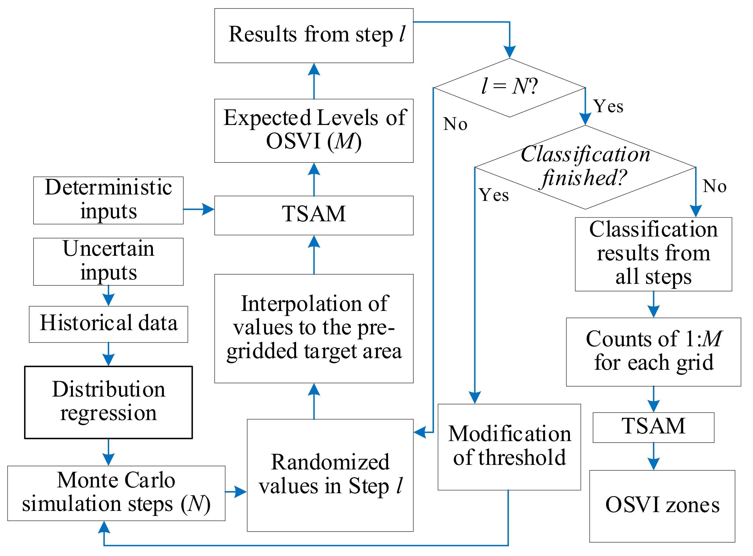
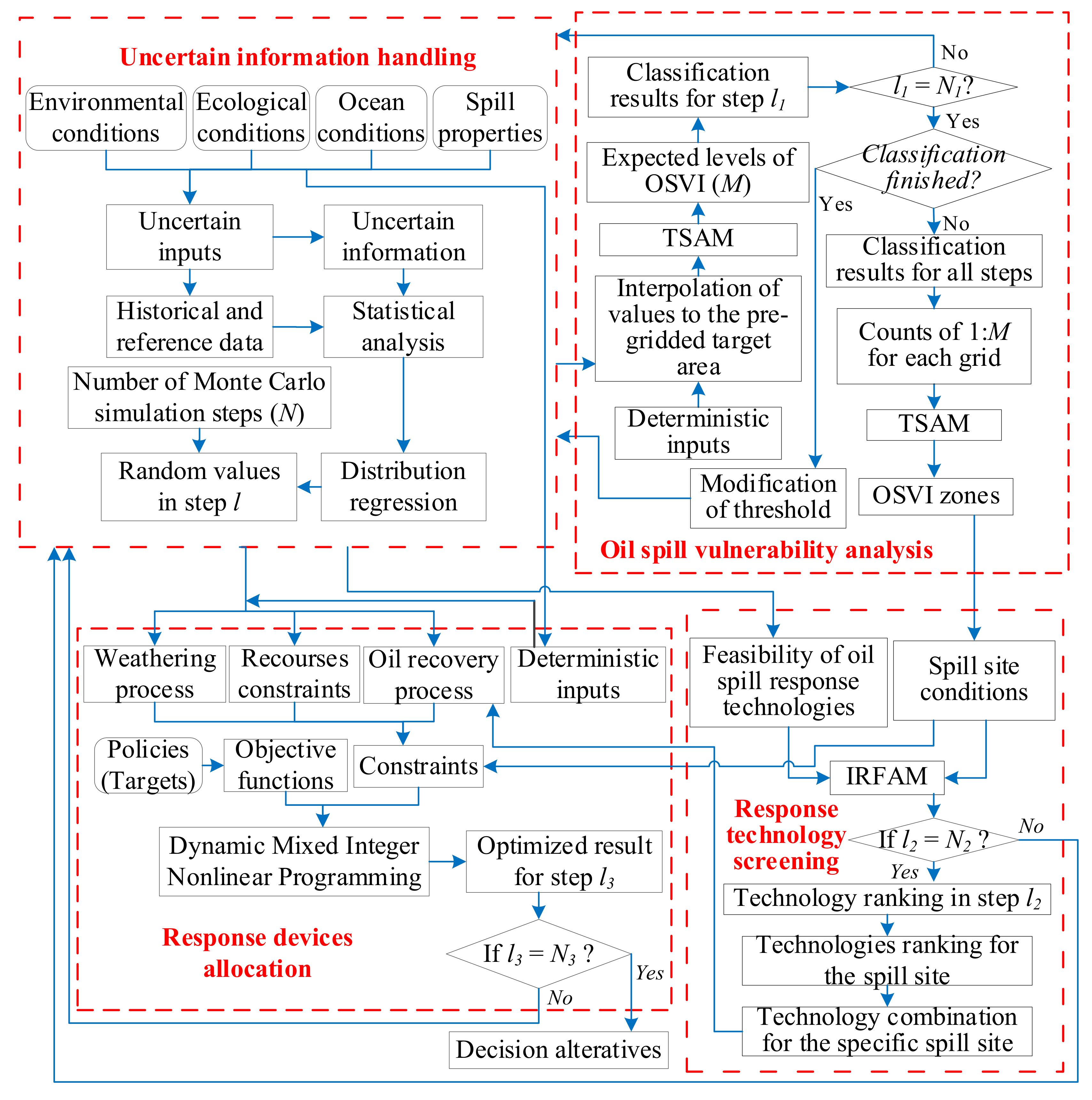
To address above concerns, the authors have previously developed an MC-TSAM approach for OSVI determination and risk zone classification [30,31]. This approach was an advance of the TSAM approach which was also previously developed by the authors based on the adaptive resonance theory (ART) and the ART mapping (ARTMap) neural network [32,33]. The framework of MC-TSAM is shown in Figure 1, where N is the total number of the Monte Carlo simulation, and l is one of the Monte Carlo simulation steps. The approach can process inputs with a mixture of deterministic and uncertain values. For the uncertain inputs, such as current and wind speeds, distributions with best fitness were first generated according to distribution regression on historical data. Accordingly, the statistics of distributions were summarized and applied to the Monte Carlo simulation for randomized number generation. In each step of Monte Carlo simulation (step l), one set of randomized numbers, as well as the deterministic values, were interpolated to the preset grids of the target area and then fed to the TSAM for OSVI analysis. With a number (e.g., N) of Monte Carlo simulation steps, the MC-TSAM is able to provide reasonable OSVI classification for a target area with consideration of complexity and uncertainty.

2.2. Offshore Oil Spill Response Technology Screening

Another challenge in offshore oil spill management is the selection of response technologies to achieve optimized response efficiency. The selection of offshore oil spill technology needs to consider a complex combination of features, including oil properties and oceanic and environmental conditions, as well as the oil weathering processes. In addition, the response technologies classification for a specific spill site also needs to consider the interaction between the efficiency of technology and the conditions of the area where the response is to be conducted. Although a number of offshore oil spill response technologies have been developed, their efficiencies in treating different types of spills significantly vary. In addition, response technology may also have uncertain feasibility and/or efficiency under uncertain site conditions, such as seawater temperature and wind and current speed, as well as the change of viscosity and density of spills. Nevertheless, current practices in response technology selection are still based on experience, which may compromise the efficiency of spill response. Only a few preliminary attempts have been made for the screening of offshore oil spill technologies on scientific basis [22,34]. Thus, classifying/ranking numerous technologies for offshore oil spill response is still difficult and challenging.

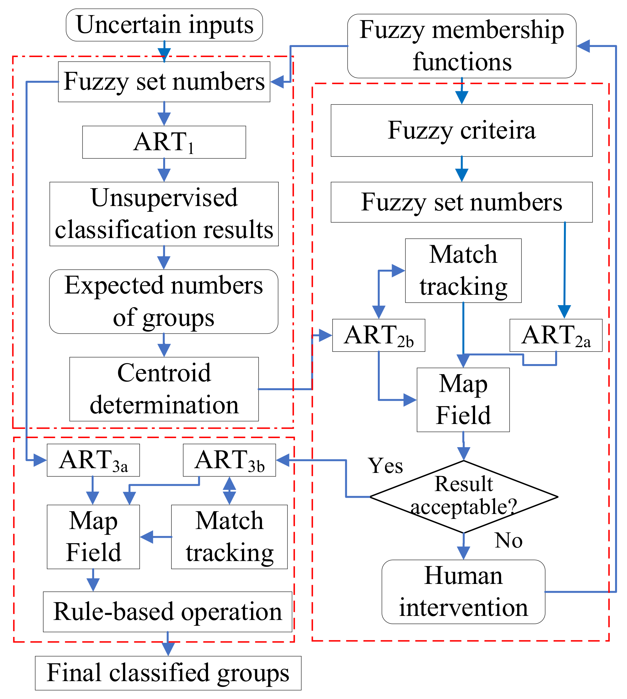
As one type of artificial neural network, the ARTMap approach has high potential for offshore oil spill technology screening. The ARTMap is a supervised classification approach. Its main modules include ART_a, ART_b and the F_ab, which are developed to process patterns, criteria and their comparisons, respectively [35]. Accordingly, the ARTMap can efficiently classify a set of data with a certain degree of complexity by a given set of criteria. However, there are practical difficulties in directly applying the original ARTMap for a classification with complex and uncertain features. The environmental conditions (e.g., seawater temperature, wave energy, wind speed and direction), oil spill properties (e.g., slick thickness and oil viscosity) and efficiency of technology are usually uncertain. Furthermore, the uncertainty is significantly amplified when the interaction in features is engaged. To reflect and handle these uncertainties and address the difficulty from the original ARTMap model, the introduction of fuzzy set theory with membership or fuzzy set generation becomes necessary [32,33].

To address the above challenge, the authors integrated the ART/ARTMap model and fuzzy set theory to develop an integrated, rule-based fuzzy adaptive resonance theory mapping (IRFAM) approach (Figure 2) [32,33]. Such an approach can efficiently handle the classification with the coexistence of complexity and uncertainty. In the IRFAM approach, the original inputs with uncertain conditions are firstly fuzzified based on the fuzzy set theory. The fuzzified inputs are then classified by unsupervised classification with ART₁. Based on the desired number of the final group by the method described in the TSAM approach [33], as well as the centroid determination module, the criteria combinations generated by the fuzzy set generation module are finally classified.

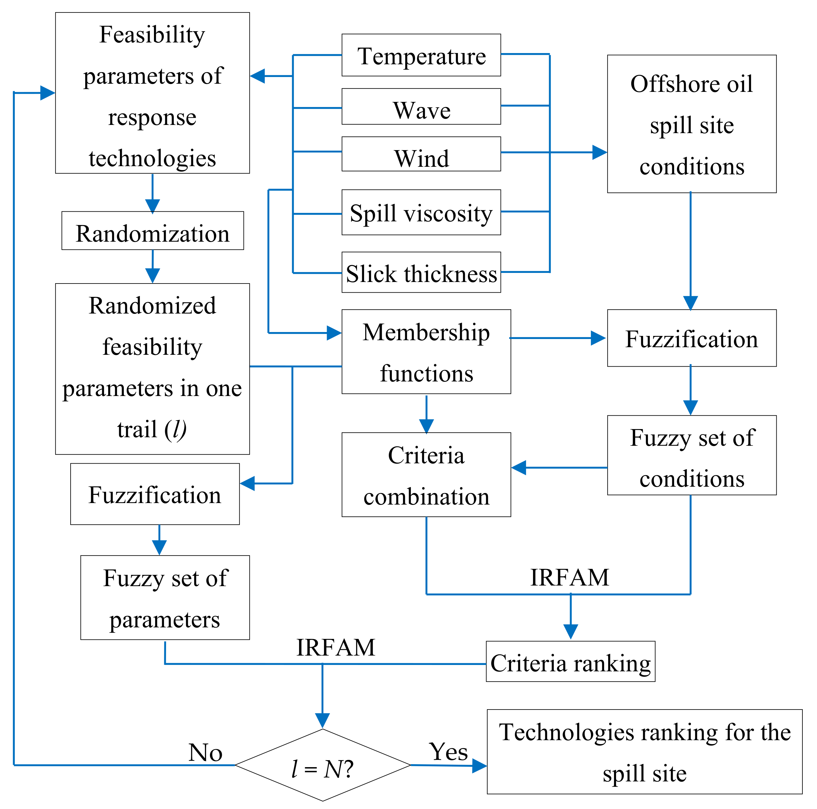
In order to address the uncertainties of data, the IRFAM approach was further advanced in this study, by coupling with a Monte Carlo simulation, yielding a Monte Carlo simulation-based IRFAM (MC-IRFAM) approach (Figure 3). This approach can produce random numbers based on the feasibility range of parameters with distribution regression. Accordingly, the availability and feasibility of response technologies can be screened and ranked based on the spilled site conditions. With a certain number of Monte Carlo simulation steps, the overall score reflecting the feasibility of the technologies can also be generated.

2.3. Simulation-Optimization Coupling for Offshore Oil Spill Response

Since offshore oil spills always cause severe impacts to the marine environment and ecosystem, an emergency response is usually initiated immediately to clean the spill and protect sensitive areas nearby. The oil spill response is usually carried out with a complicated combination of interactive processes such as dispersion by chemical dispersants, containment and recovery by booms and skimmers and combustion by in-situ burning [36]. The effectiveness of response is significantly affected by various uncertain environmental conditions and spill properties, including seawater temperature, wave energy, wind speed and direction, oil density and viscosity, slick thickness, etc. These uncertain conditions lead to difficulties in real-time decisions for response actions and resource allocation during an offshore oil spill. The coupling of simulation and optimization for these processes under varying circumstances can be significantly helpful to the oil spill response. However, it is a challenging task, and few attempts have been reported [31,34].

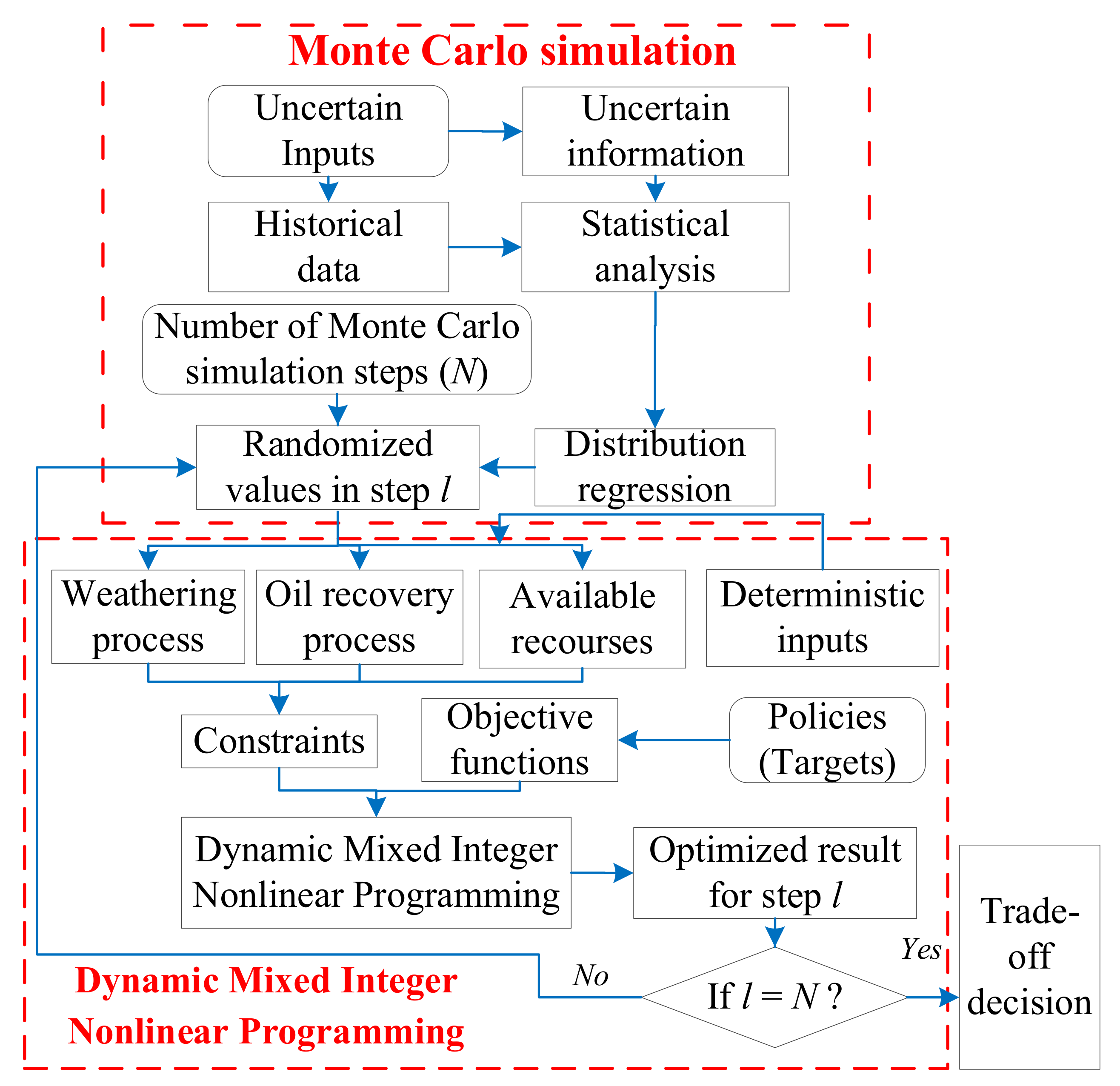
To address the above concern, a Monte Carlo simulation-based, dynamic, mixed-integer nonlinear programming (MC-DMINP) approach was previously developed by the authors to effectively and dynamically support offshore oil spill response [37,38]. The general framework of the MC-DMINP is shown in Figure 4. In each Monte Carlo simulation step, a set of random values is generated based on the regressed distribution of uncertain parameters, converting the uncertain problem to a deterministic one at this step. With the completion of all Monte Carlo simulation steps, the distribution of solutions is generated and further analyzed with a trade-off decision.

In each Monte Carlo simulation step, a general simulation-optimization coupling model is generated with consideration of oil recovery (e.g., skimming) and weathering simulation:

$$Max\hspace{1em}{V}_{rec}={\displaystyle \sum }_{s=1}^N{\displaystyle \sum }_{j=1}^{M}S{K}_j\times OR{R}_{nsj}$$

(1)

$$OR{R}_{nis}=f_{OR{R}_{ni}}\left(\frac{V_0-{{\displaystyle \sum }}_{h=1}^{s-1}\left(V_h+F{V}_h+D{V}_h\right)}{A}\right)$$

(2)

$$D{E}_s=f_{FD}\left(SO{T}_{s-1}, {\mu }_s^o\right)=f_{DE}\left(\frac{V_0-{{\displaystyle \sum }}_{h=1}^{s-1}\left(V_h+F{V}_h+D{V}_h\right)}{A}, {\mu }_{s-1}^o\right)$$

(3)

$${\mu }_s^o=f_{\mu }\left({\mu }_{s-1}^o, F{E}_{s-1}, F{W}_{s-1}\right)$$

(4)

$$F{V}_s=F{E}_{s-1}\times \left(V_0-{\displaystyle \sum }_{h=1}^{s-1}\left(V_h+F{V}_h+D{V}_h\right)\right)$$

(5)

$$D{V}_s=D{E}_{s-1}\times \left(V_0-{\displaystyle \sum }_{h=1}^{s-1}\left(V_h+F{V}_h+D{V}_h\right)\right)$$

(6)

$${\displaystyle \sum }_{j=1}^{M}S{K}_j\le B$$

(7)

$$S{K}_j\ge 0$$

(8)

where V_rec is the recovered oil volume (m³); SK_j is the number of response devices (e.g., skimmer); ORR_ni is the oil recovery rate (m³/h); N is the oil spill response window (h); s is the step index of the response window; M is the types of response technologies; V₀ is the initial volume of spilled oil (m³); V_h, FV_h and DV_h are the volumes of remained, evaporated and dispersed oil (m³) at step h; A is the spilled oil area (km²), h is the step index, $\mu$ is the oil dynamic viscosity (cP); FE, FW and DE are the evaporation, emulsification and dispersion rate of the oil (m³/(s∙m³ of oil)); B is the capacity of the vessels carrying the response technologies.

2.4. Integrated Decision Support System for Offshore Oil Spill Management

Based on the developed MC-TSAM, MC-IRFAM and MC-DMINP, an integrated decision support system was developed for offshore oil spill management, named DSS-OSM. As shown in Figure 5, the integrated DSS utilized the Monte Carlo simulation to generate random values for uncertain inputs in all the processes during offshore oil spill management. Correspondingly, the randomized inputs were fed to the TSAM, IRFAM and DMINP for offshore oil spill vulnerability analysis and spill alert, oil spill response technology screening and ranking and devices and equipment allocation during offshore oil spill actions. Eventually, the DSS-OSM can provide integrated decision support to offshore oil spill management.

3. A Case Study of Offshore Oil Spill Management

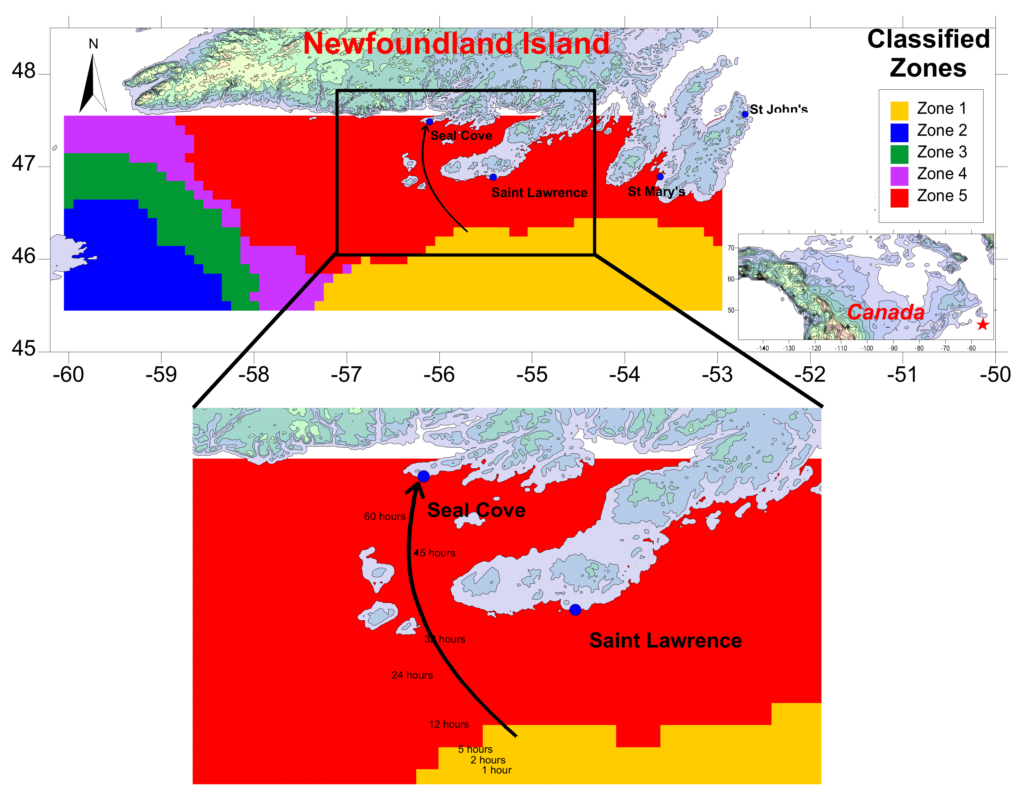
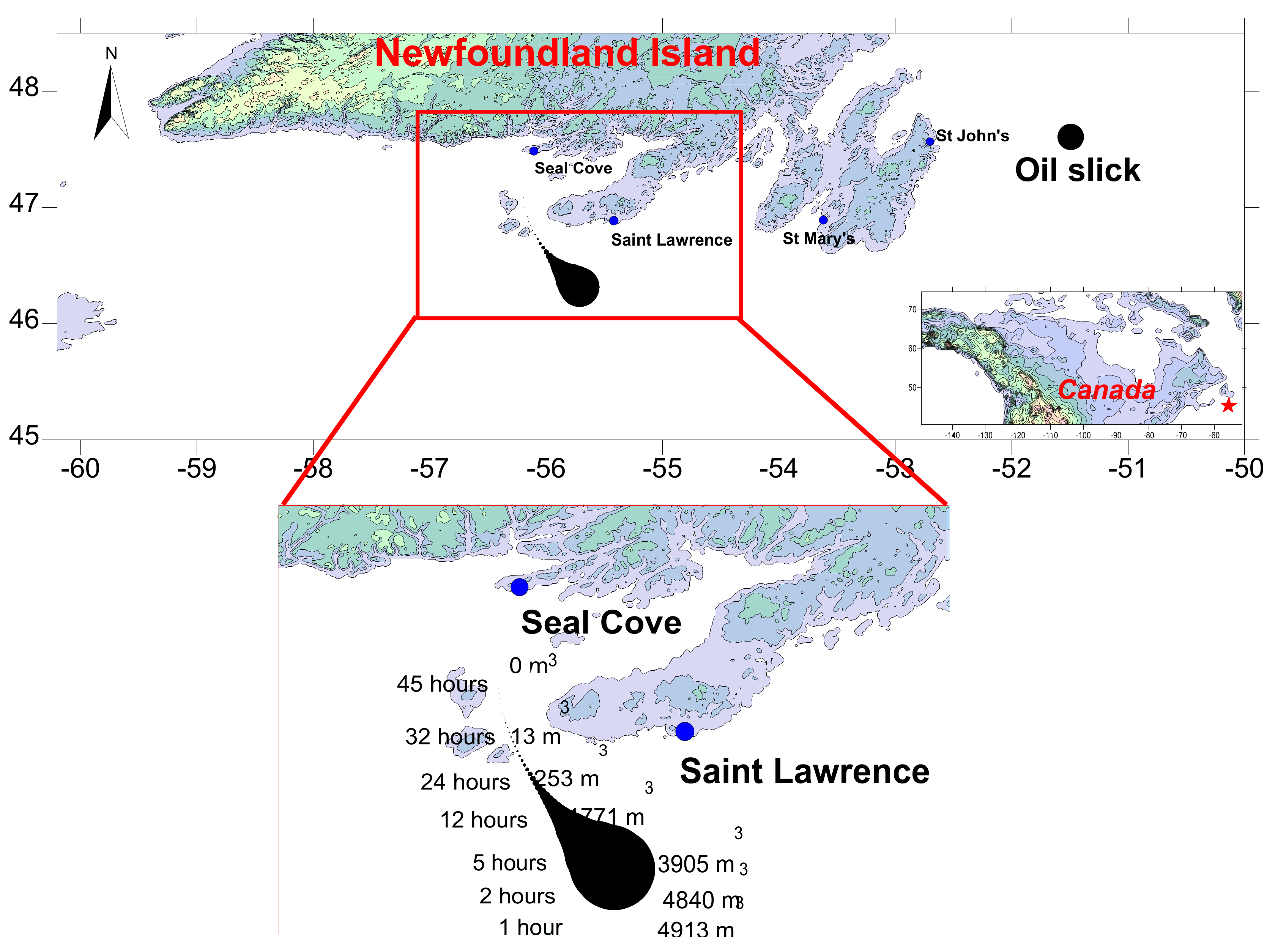
A case study regarding decision support to offshore oil spill management was conducted to demonstrate the feasibility and efficiency of the developed DSS-OSM. The region in the case study was the south coast of Newfoundland (53° W to 60° W, 45.5° N to 47.5° N). For modeling purposes, the region was pre-gridded with 0.1° by 0.1° cells.

3.1. Offshore OSVI Classification

The details of the OSVI classification can be found in the authors’ previous study [31]. The inputs included (1) meteorological information: seawater temperature (°C), wind speed (m/s), wind direction (degree) and pressure (mb); (2) oceanographical information: current speed (m/s), current direction (degree) and wave energy/height (m); (3) ecological information: density of spawning fish (/520 m²) and location of ecological reserves; and (4) oil spill relative information: oil spill frequency in the past (/year), density of tanker transport (/year) and density of other vessel transport (/year). Based on the MC-TSAM module, the OSVI in the target area was classified into Zone 1 to 5 with increasing vulnerability to offshore oil spill [31]. The distributions of each parameter in each zone are listed in Figures S1–S10 in the Supplementary Materials.

The OSVI classification results were further analyzed to provide summaries of the site conditions for response technology screening based on MC-IRFAM and response devices/equipment allocation based on MC-DMINP.

3.2. Simulation of Oil Slick Movement

The spilled oil in this case study was the Statfjord crude which is one of the most popular crude oils that is transported worldwide (

Table 1. Oil properties of Statfjord crude [40].

Parameter	Value	Parameter	Value
Vapor pressure	10.4 Pa	Molecular weight	128.2 g/mol
Density	832 kg/m3	Gas constant	8.314 m3∙Pa/mol∙K
Viscosity	3.03 cP	Interface tension	2000 dyne/m

). The spill location was set to 55.7° W and 46.3° N, where the highest density of marine-time traffic appeared in the region [39]. The total spill volume was 5000 m³. It was assumed that a set of booms had been applied to confine the spill area to 100,000 m², yielding a slick thickness of 50 mm at the initial stage.

To estimate the oil slick trajectory, the following model was firstly applied [41,42]:

$$\overrightarrow{V}={\overrightarrow{V}}_c+\overrightarrow{V^{\prime }}$$

(9)

where $\overrightarrow{V}$ is the velocity of oil slick advection (m/s) during each time step; ${\overrightarrow{V}}_c$ is the average velocity of oil slick advection (m/s) due to the combined effect from current and wind; and $\overrightarrow{V^{\prime }}$ is the velocity of oil slick advection affected by turbulent fluctuation (m/s). For simplification, the effect of turbulent fluctuation was ignored in this case study. Correspondingly, the velocity of oil slick advection was calculated as follows: [43,44,45,46]:

$$\overrightarrow{V}={\overrightarrow{V}}_c$$

(10)

In addition, the longitude and latitude were approximated to the preset grids. For example, x₀ = −55.7 and y₀ = 46.3 were set for the initial spill location. Accordingly, the trajectory of the spill slick was simulated as follows:

$$x_t=x_{t-1}-\frac{cos\left(c{d}_{t-1}\right)\times c{s}_{t-1}\times 60}{LX}$$

(11)

$$y_t=y_{t-1}+\frac{sin\left(c{d}_{t-1}\right)\times c{s}_{t-1}\times 60}{LY}$$

(12)

where cs_t−1 and cd_t−1 are the speed (m/s) and direction (degree) of current at time step t − 1, respectively; x_t and y_i are latitudinal and longitudinal moving direction (degree) of the spill at time t, respectively; x_t−1 and y_i−1 are latitudinal and longitudinal location (degree) of the spill from the previous simulation step (t − 1), respectively; LX = 7724 m and LY = 11,120 m represent the distance of 1º longitude and latitude in the study area, respectively [47].

The wind and current field data were downloaded from the GOODS (GNOME Online Oceanographic Data Server) of the National Oceanic and Atmospheric Administration (NOAA). According to Equations (10)–(12), as well as the wind and current field data, the trajectory of the spill slicks was simulated with a time step of 1 min and a simulation window of 60 h. The result is shown in Figure 6, which indicates that if no response action was applied, the spilled oil would contaminate the shoreline area of Newfoundland about 60 h after the release.

3.3. Offshore Oil Spill Response Technology Screening

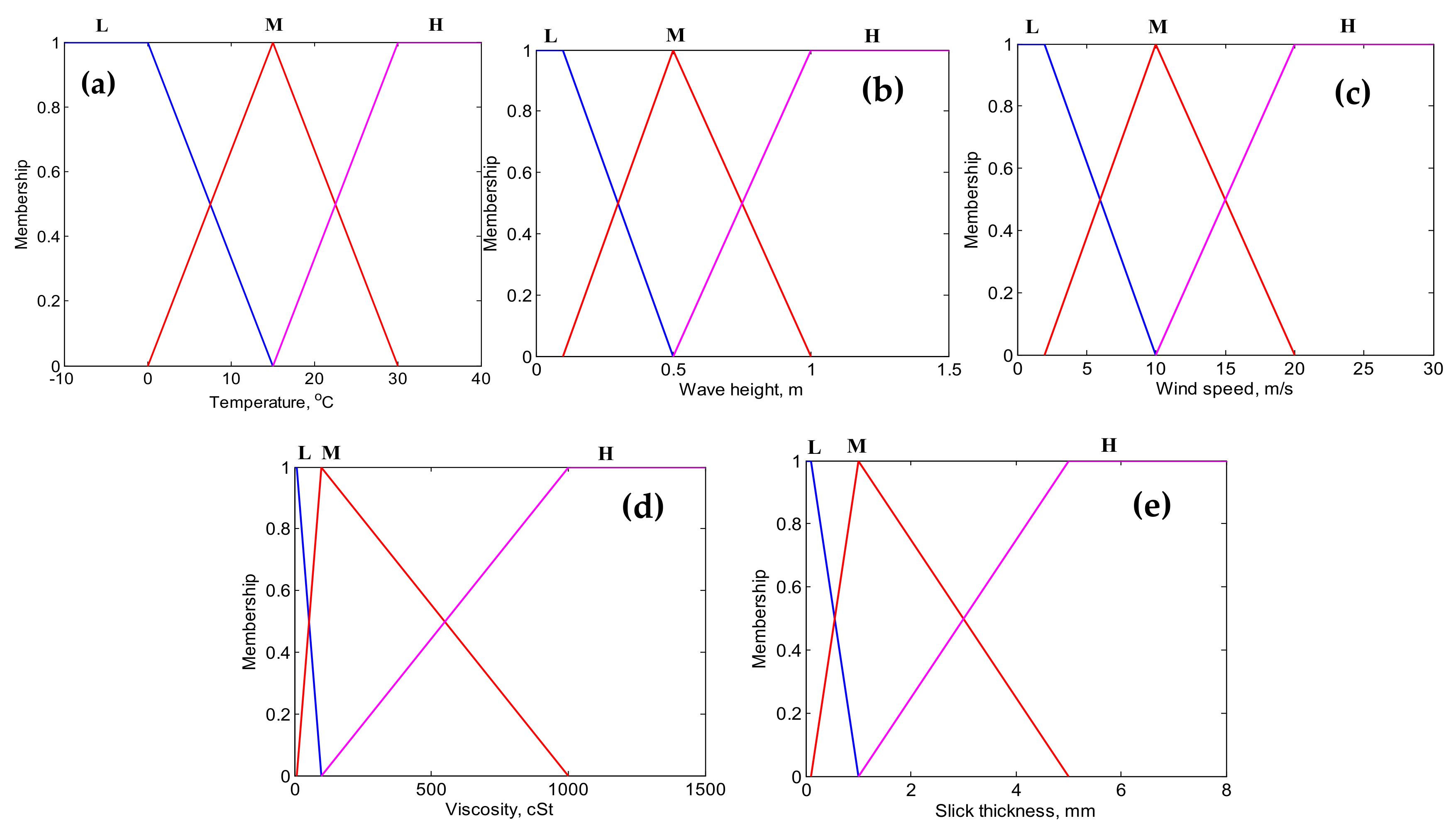
Based on the 60 h simulation of oil slick trajectory, the spill would enter Zone 5 in about 2 h and reach the shoreline area of Newfoundland about 60 h after the release. As a result, the offshore oil spill response needed to be conducted in Zones 1 and 5, which appear to have different site conditions. The feasibility parameters of response technologies (e.g., skimmer) included seawater temperature, wind speed, wave energy/height and oil properties (i.e., viscosity and slick thickness). Accordingly, the fuzzy membership functions for these parameters were generated (Figure 7).

The distributions of the site conditions for Zones 1 and 5 are listed in Figures S1, S2 and S5 in the Supplementary Materials. Accordingly, the mean and 95% confidence interval for the site conditions of these two zones, as well as the operational conditions of different types of available skimmers, are summarized (

Table 2. Information of site conditions and skimmer feasibilities.

	Seawater Temperature °C	Wave Height m	Wind Speed m/s	Oil Viscosity cP	Slick Thickness mm
Zone 1	0–15	0.5–5	3–13	≥3.03	≤50
Zone 5	−5–20	0.2–4	0.5–15	≥3.03	≤0
SK 1	≥−10	0–3	0–20	≥10	5–50
SK 2	−10–20	0–2.5	0–15	≥5	1–50
SK 3	−5–15	0–2	0–12	≥2	0–50
SK 4	5–20	0–0.5	≥20	10–200	0.01–1
SK 5	20–30	0.5–2	0–5	50–1000	1–5
SK 6	≥30	0–0.2	≥10	≥1000	≥4
SK 7	10–15	0–0.3	0–10	≥50	0.1–0.5

Note: SK—Skimmer.

). According to the fuzzy member functions listed in Figure 7, these values were fuzzified and fed to the MC-IRFAM for technology screening and ranking with 10,000 Monte Carlo simulation steps. The output was a series of overall scores (ranged from 0 to 1), representing the feasibility of skimmers. The lowest score was 0, representing an absolute unfeasibility. In contrast, the highest score was 1, representing a perfect feasibility. The score of 0.5 indicated a reasonable feasibility.

Table 3. Statistics of skimmer feasibility for offshore oil spill response in Zone 1.

Skimmer	Mean	Median	Minimum Value	Maximum Value	Lower Bound of 95% CI	Upper Bound of 95% CI
SK 1>	0.674	0.660	0.414	0.881	0.533	0.867
SK 2	0.699	0.667	0.413	0.933	0.546	0.867
SK 3	0.669	0.653	0.356	1.000	0.535	0.853
SK 4	0.544	0.544	0.399	0.666	0.467	0.624
SK 5	0.616	0.624	0.528	0.667	0.540	0.667
SK 6	0.515	0.533	0.400	0.600	0.470	0.600
SK 7	0.588	0.593	0.428	0.824	0.486	0.680

and

Table 4. Statistics of skimmer feasibility for offshore oil spill response in Zone 5.

Skimmer	Mean	Median	Minimum Value	Maximum Value	Lower Bound of 95% CI	Upper Bound of 95% CI
SK 1	0.716	0.730	0.467	0.921	0.548	0.867
SK 2	0.698	0.667	0.467	0.933	0.569	0.867
SK 3	0.659	0.653	0.364	0.933	0.543	0.800
SK 4	0.542	0.543	0.414	0.661	0.475	0.607
SK 5	0.750	0.800	0.528	0.800	0.609	0.800
SK 6	0.549	0.567	0.433	0.667	0.500	0.637
SK 7	0.592	0.602	0.458	0.809	0.504	0.649

list the statistics of the overall scores for the feasibility of available skimmers conducting offshore oil spills in Zones 1 and 5. These statistics include minimum and maximum values, median, mean and 95% conference interval (CI). According to the results, the overall score distributions, means, medians and 95% CIs for SK 1, SK 2 and SK 3 operating in Zone 1 were similar, indicating a close feasibility of these skimmers. In addition, the feasibility of these skimmers to Zone 1 was promising because most of their scores were higher than 0.5. Further comparison in the overall score distribution indicated that most of the scores of SK 3 tended to be high values, while the ones of SK 1 tended to be low values. In addition, the score tendency of SK 2 was insignificant. Although SK 5 appeared to have lower feasibility than SKs 1 to 3, it could still achieve a reasonable performance since its overall score was still higher than 0.5. SK 4 and SK 7 and had similar distribution in overall scores of feasibilities. Comparatively, the feasibility of SK 7 was slightly higher than SK 4 because the scores of SK 7 tended to be higher than the ones of SK 4. Generally, SK 6 might not be feasible for the oil spill response in this case. As a summary, the ranks of skimmer feasibility for offshore oil spill response in Zone 1 were SK 3 > SK 2 > SK 1 > SK 5 > SK 7 > SK 4 > SK 6.

The feasibility ranking for the skimmers operating in Zone 5 was close to those in Zone 1, excluding the following differences: (1) SK 2 appeared to have the highest feasibility, followed by SK 1, then SK 3; and (2) the feasibility of SKs 5 to 7 appeared to slightly increase. In general, the ranks of skimmer feasibility for offshore oil spill response in Zone 5 were SK 2 > SK 1 > SK 3 > SK 5 > SK 7 > SK 4 > SK 6.

3.4. Response Devices/Equipment Allocation

In decision support to the response devices/equipment allocation, three types of skimmers (SK 1, SK 2 and SK 3) were selected based on their highest ranks from the technology screening and ranking process. The oil recovery rates of these skimmers had quadratic relationships with the oil slick thickness as follows:

$$OR{R}_n=aS{T}^2+bST$$

(13)

where ORR_n is the oil recovery rate for skimmer (m³/h), ST is the oil slick thickness (mm) and a and b are coefficients based on experiments.

There were three warehouses nearby (Saint Lawrence, St Mary’s and St John’s) that held eight sets of skimmers for each type. Due to the different distances from each warehouse to the spill site, the times for deploying different types of skimmer were different. The coefficients for skimmers and the time required for their deployment are listed in

Table 5. Time for device deployment and parameters for ORRn simulation.

Skimmer	Time for Device Deployment (h)	Parameter for ORRn Simulation
		a	b
SK 1	3	0.01437	0.01602
SK 2	6	−0.00791	0.84975
SK 3	12	−0.01591	1.54975

. In addition, the total capacity of vessels for holding the devices was 20 sets of skimmers.

Due to the previous simulation of oil slick trajectory, if no offshore oil spill response was applied, the spill would contaminate the shoreline area of Newfoundland 60 h after the release (Figure 6). Correspondingly, the target of the oil spill response was to perform a fast and effective clean-up of the spilled oil within 60 h. Furthermore, no additional device would be applied during this period due to the challenges in distance and transportation.

According to the wind speed and temperature distribution of Zone 1 and Zone 5 (Figures S2 and S5 in the Supplementary Materials), a Monte Carlo simulation model was developed. In addition, a normal distribution with 100,000 m² mean value and 8000 m² standard deviation was assumed for the slick area. The Monte Carlo simulation steps were set to 200. In each step, a simulation-optimization coupling approach based on the MC-DMINP was developed for the combination and allocation of skimmers:

$$Max\hspace{1em}V={\displaystyle \sum }_{m=1}^{60}{V}_m$$

s.t.

$$\begin{array}{l}{V}_1={\displaystyle \sum _{j=1}^3}S{K}_j\times OR{R}_{njm}=bs{k}_{1m}\times S{K}_1 \hspace{1em}\hspace{1em}\hspace{1em}\hspace{1em}\hspace{1em}\hspace{1em}\hspace{1em}\forall m=1\\ \hspace{1em}\hspace{1em}\hspace{1em}\hspace{1em}\hspace{1em}\hspace{1em}\hspace{1em} \times \left(0.01437{\left(\mathrm{1,000}\frac{V_0}{A}\right)}^2+0.01602\left(\mathrm{1,000}\frac{V_0}{A}\right)\right)\\ \hspace{1em}\hspace{1em}\hspace{1em}\hspace{1em}\hspace{1em}\hspace{1em}\hspace{1em} +{bsk}_{2m}\times S{K}_2\\ \hspace{1em}\hspace{1em}\hspace{1em}\hspace{1em}\hspace{1em}\hspace{1em}\hspace{1em}\times (-0.00791{\left(\mathrm{1,000}\frac{V_0}{A}\right)}^2 +0.84975\left(\mathrm{1,000}\frac{V_0}{A}\right))\\ \hspace{1em}\hspace{1em}\hspace{1em}\hspace{1em}\hspace{1em}\hspace{1em}\hspace{1em} +bs{k}_{3m}\times S{K}_3\\ \hspace{1em}\hspace{1em}\hspace{1em}\hspace{1em}\hspace{1em}\hspace{1em}\hspace{1em} \times \left(-0.01591{\left(\mathrm{1,000}\frac{V_0}{A}\right)}^2+1.54975\left(\mathrm{1,000}\frac{V_0}{A}\right)\right)\end{array}$$

(14)

$$F{E}_1=\frac{2.67+0.06\times \left(T-273.15\right)\times Ln\left(60\right)}{100}\hspace{1em}\forall m=1$$

(15)

$$D{E}_1=\frac{0.11{\left(U+1\right)}^2}{1+50{\mu }_0^o{}^{0.5}\left(\frac{V_0}{A}\right)s_t}\hspace{1em}\hspace{1em}\hspace{1em}\hspace{1em}\forall m=1$$

(16)

$$V{F}_1=V_0\times F{E}_1\hspace{1em}\hspace{1em}\hspace{1em}\hspace{1em}\hspace{1em}\hspace{1em}\hspace{1em}\hspace{1em}\forall m=1$$

(17)

$$V{D}_1=V_0\times D{E}_1\times 3.600\hspace{1em}\hspace{1em}\hspace{1em}\hspace{1em}\hspace{1em}\forall m=1$$

(18)

$$\begin{array}{l}{V}_m={\displaystyle \sum _{j=1}^3}S{K}_j\times OR{R}_{njm} \hspace{1em}\hspace{1em}\hspace{1em}\hspace{1em}\hspace{1em}\hspace{1em}\hspace{1em}\forall m=2,\cdots ,60\\ \hspace{1em}\hspace{1em}\hspace{1em}\hspace{1em}\hspace{1em}\hspace{1em}\hspace{1em}=bs{k}_{1m}\times S{K}_1\\ \hspace{1em}\hspace{1em}\hspace{1em}\hspace{1em}\hspace{1em}\hspace{1em}\hspace{1em}\times (0.01437{\left(\frac{\mathrm{1,000}\left(V_0-{{\displaystyle \sum }}_{h=1}^{m-1}{V}_h\right)}{A}\right)}^2\\ \hspace{1em}\hspace{1em}\hspace{1em}\hspace{1em}\hspace{1em}\hspace{1em}\hspace{1em}+0.01602\left(\frac{\mathrm{1,000}\left(V_0-{{\displaystyle \sum }}_{h=1}^{m-1}{V}_h\right)}{A}\right))\\ \hspace{1em}\hspace{1em}\hspace{1em}\hspace{1em}\hspace{1em}\hspace{1em}\hspace{1em}+bs{k}_{2m}\times S{K}_2\\ \hspace{1em}\hspace{1em}\hspace{1em}\hspace{1em}\hspace{1em}\hspace{1em}\hspace{1em}\times (-0.00791{\left(\frac{\mathrm{1,000}\left(V_0-{{\displaystyle \sum }}_{h=1}^{m-1}{V}_h\right)}{A}\right)}^2\\ \hspace{1em}\hspace{1em}\hspace{1em}\hspace{1em}\hspace{1em}\hspace{1em}\hspace{1em}+0.84975\left(\frac{\mathrm{1,000}\left(V_0-{{\displaystyle \sum }}_{h=1}^{m-1}{V}_h\right)}{A}\right))\\ \hspace{1em}\hspace{1em}\hspace{1em}\hspace{1em}\hspace{1em}\hspace{1em}\hspace{1em}+bs{k}_{3m}\times S{K}_3\\ \hspace{1em}\hspace{1em}\hspace{1em}\hspace{1em}\hspace{1em}\hspace{1em}\hspace{1em}\times (-0.01591{\left(\frac{\mathrm{1,000}\left(V_0-{{\displaystyle \sum }}_{h=1}^{m-1}{V}_h\right)}{A}\right)}^2\\ \hspace{1em}\hspace{1em}\hspace{1em}\hspace{1em}\hspace{1em}\hspace{1em}\hspace{1em}+1.54975\left(\frac{\mathrm{1,000}\left(V_0-{{\displaystyle \sum }}_{h=1}^{m-1}{V}_h\right)}{A}\right))\end{array}$$

(19)

$$F{E}_m=\frac{2.67+0.06\times \left(T-273.15\right)\times Ln\left(60\right)}{100} \forall m=2,\cdots ,60$$

(20)

$$D{E}_m=\frac{0.11{\left(U+1\right)}^2}{1+50{\mu }_m^o{}^{0.5}\left(\frac{V_0-{{\displaystyle \sum }}_{h=1}^{m-1}\left(V_h+V{F}_h+V{D}_h\right)}{A}\right)s_t}\hspace{1em}\forall m=2,\cdots ,60$$

(21)

$$F{W}_m=K_b\left(1-exp\left(\frac{-K_a}{K_b}\right){\left(U+1\right)}^2\times 3.600\right)\hspace{1em}\forall m=2,\cdots ,60$$

(22)

$${\rho }_m^o=F{W}_{m-1}{\rho }_w+\left(1-F{W}_{m-1}\right)\left({\rho }_{m-1}^o+K_{b}F{E}_{m-1}\right)\hspace{1em}\forall m=2,\cdots ,60$$

(23)

$${\mu }_m^o={\mu }_{m-1}^{o}exp\left(K_{c}F{E}_{m-1}\right)exp\left(\frac{2.5F{W}_{m-1}}{1-K_{b}F{W}_{m-1}}\right)\hspace{1em}\forall m=2,\cdots ,60$$

(24)

$$V{F}_m=V_0\times F{E}_m\hspace{1em}\hspace{1em}\forall m=2,\cdots ,60$$

(25)

$$V{D}_m=V_0\times D{E}_m\times 3.600\hspace{1em}\hspace{1em}\forall m=2,\cdots ,60$$

(26)

$${\displaystyle \sum }_{j=1}^{3}S{K}_j\le 20$$

(27)

$$0\le S{K}_j\le 8\hspace{1em}\forall j=1, 2, 3$$

(28)

$$bs{k}_{jm}=0\hspace{1em}\hspace{1em}\forall j=1, 2, 3; \forall t{t}_j>m$$

(29)

$$bs{k}_{jm}=1\hspace{1em}\hspace{1em}\forall j=1, 2, 3; \forall t{t}_j\le m$$

(30)

$$S{K}_j\in integer\hspace{1em}\forall j=1, 2, 3$$

(31)

where V is the total volume of collected oil (m³); V_m and V_h are the collected volume of oil in each 1 h time step (m³); m and h are the time step indices (m > h); j is the skimmer type index; ORR_n is the net oil recovery rate (m³/h); bsk_jm is the binary indicator which indicates whether SK_j is applied in the oil spill response at stage m; V₀ is the release volume of spilled oil at the beginning (m³); T is the seawater temperature (K); S_t is the oil–water interfacial tension (dyne/m); U is the wind speed (m/s); K_a is a cure fitting constant (2 × 10⁻⁶); K_b is the constant for mousse viscosity (0.7) [47]; ${\rho }_w$ is the seawater density (kg/m³); ${\rho }^o$ is the initial density of oil (kg/m³); $K_c$ is a constant between 1 and 10 (1 for light refined oil and 10 for crudes); and tt_j is the time for SK_j allocation and deployment.

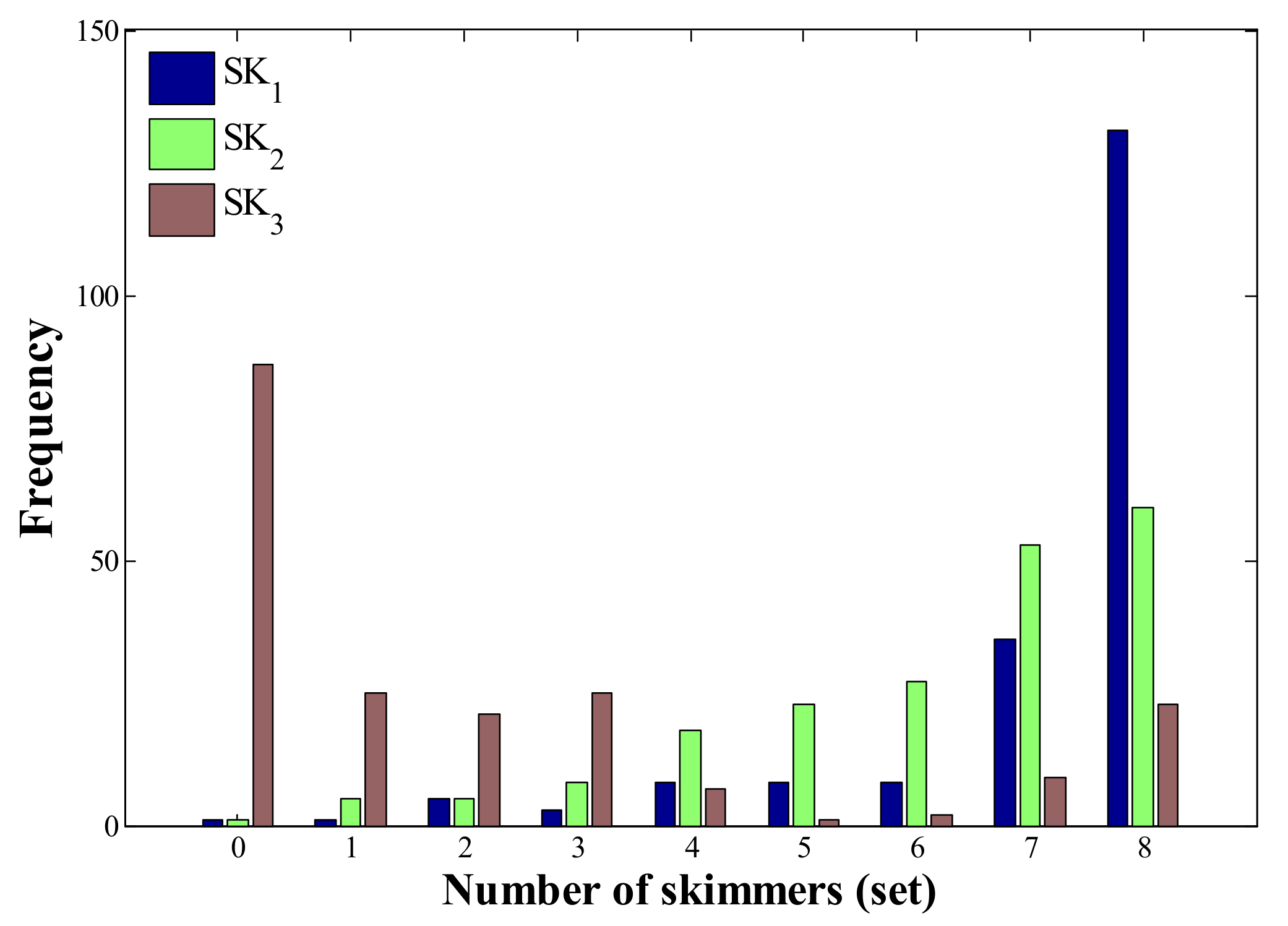
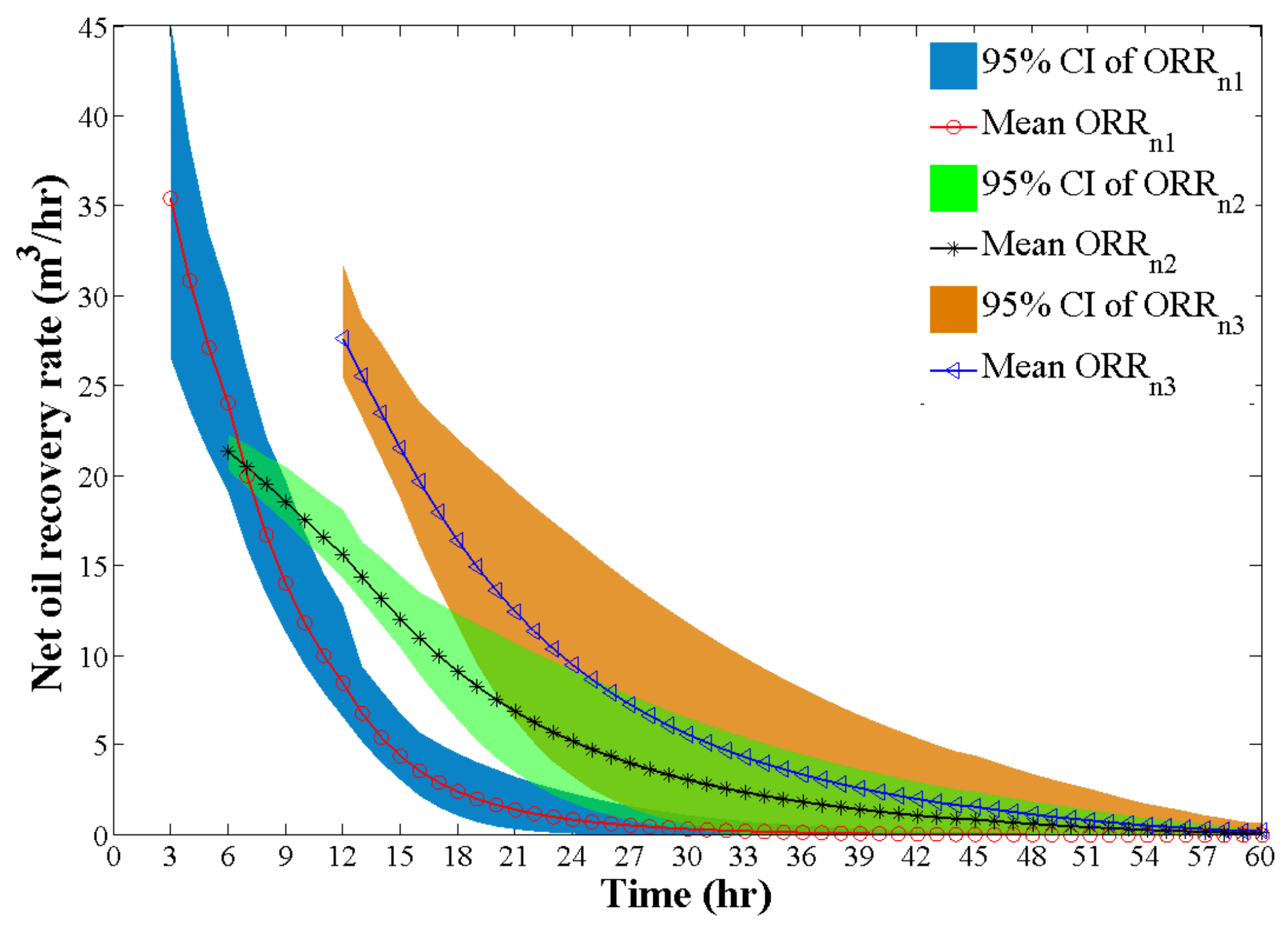
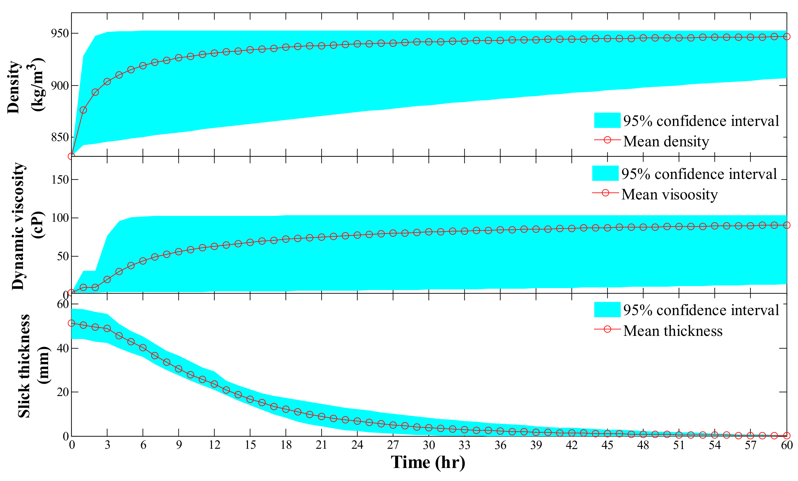
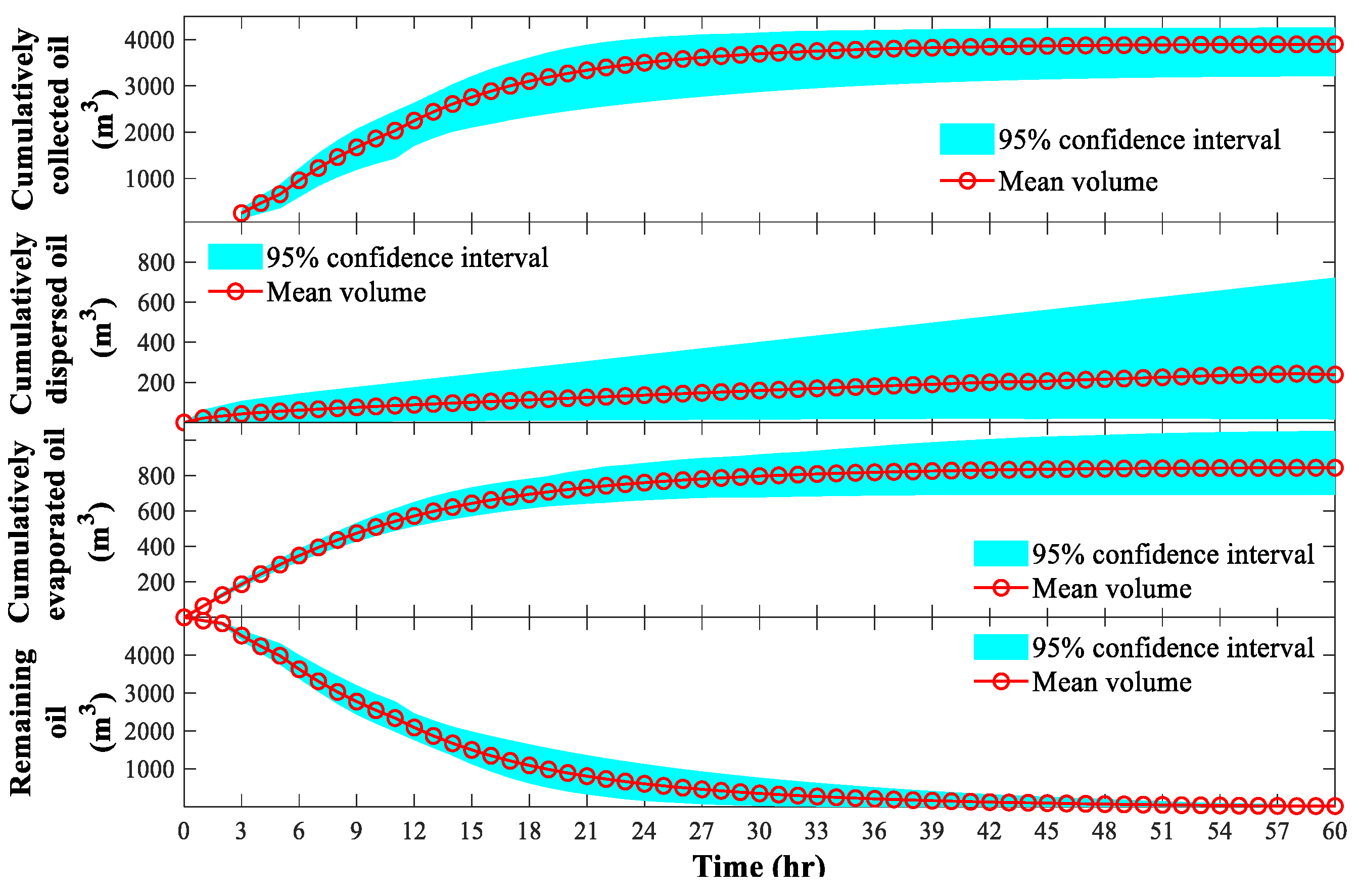
The MC-DMINP modeling results are illustrated in Figure 8, Figure 9, Figure 10, Figure 11, Figure 12, Figure 13, Figure 14, Figure 15 and Figure 16. The distributions of skimmer numbers indicated the highest probability of deployed SK₁ and SK₂ were eight sets and the number of SK₃ heavily depended on the vacancy of the vessel capacity (Figure 8). Since there were only eight sets of SK₁ and SK₂ in total, and the capacity of vessels was 20 sets of skimmers, the optimal combination would be SK₁: eight sets, SK₂: eight sets and SK₄: eight sets. Based on this combination and the simulation-optimization coupling approach, the transport and behavior of the spilled oil were simulated. The results indicated that most of the oil was removed from sea surface about 45 h after the release and would not reach the shoreline area of Newfoundland (Figure 9).

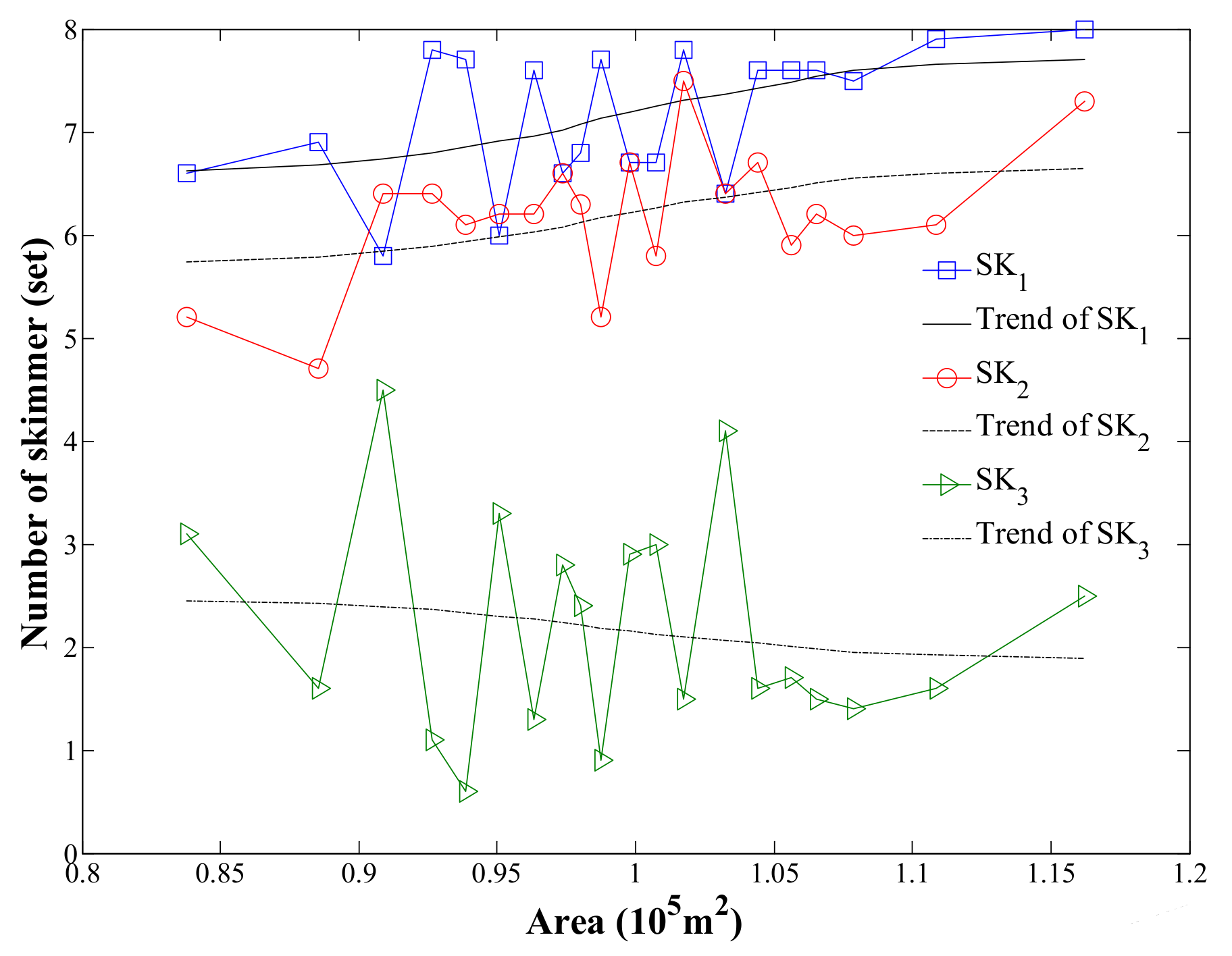
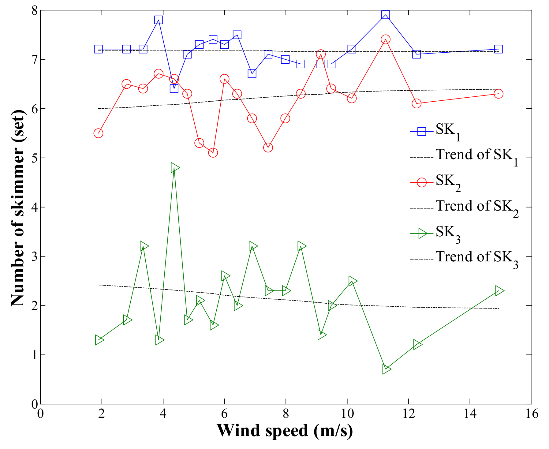
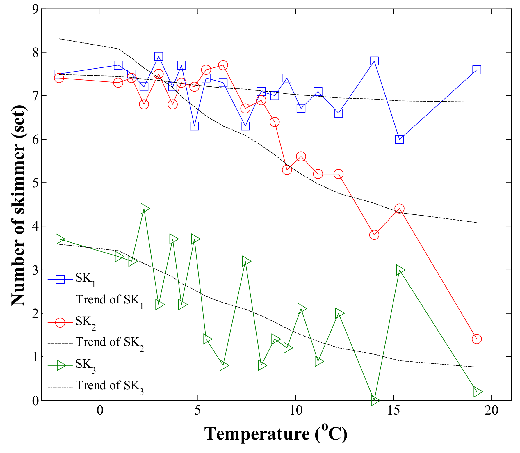
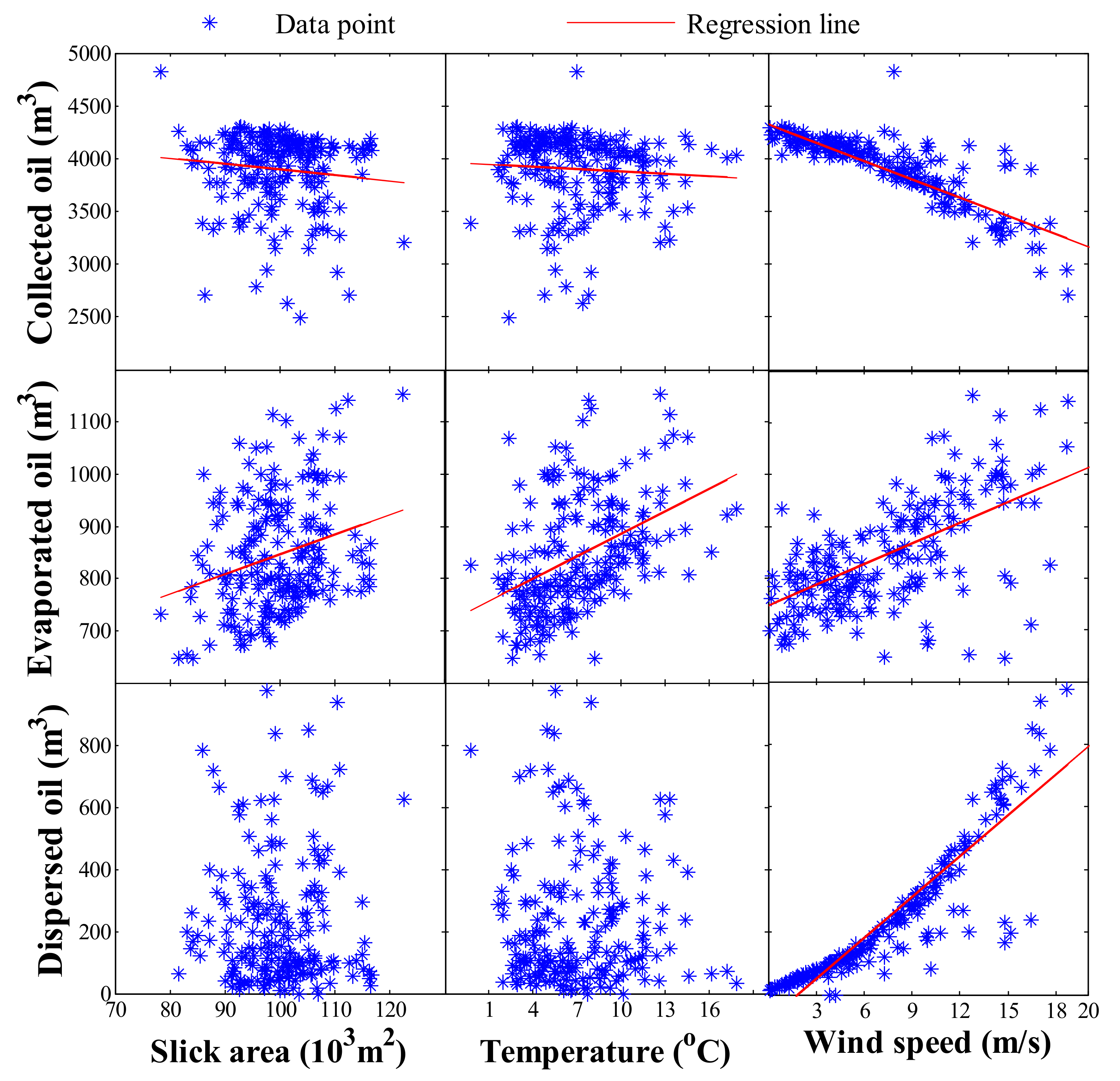
The final oil budget was 82% collection (4096 m³), 14.4% evaporation (724 m³) and 3.6% dispersion (180 m³). Figure 10, Figure 11, Figure 12, Figure 13, Figure 14 and Figure 15 show the simulation results regarding ORRn changes, oil collection, evaporation and dispersion, as well as the changes in slick thickness, oil density and viscosity. The number of SK₁ and SK₂ appeared to have significantly positive correlations with the initial slick area. The number of SK₃ appeared to have a negative correlation with the initial slick area but was not significant (Figure 13). Furthermore, the wind speed had a positive correlation with the number of SK₂ and a negative one with the number of SK₃. Its correlation with the number of SK₁ was not observed (Figure 14). Since the oil dispersion process was enhanced by strong wind 1 day (24 h) after the release (Figure 12), the skimming efficiency was significantly affected (Figure 16). As a result, SK₁ and SK₂ that required a shorter time of deployment were preferred compared to SK₃ which required a much longer time for deployment. Strong negative correlations were observed between SK₃/SK₂ and the uncertainty of seawater temperature, while the correlation between SK₁ and seawater temperature was insignificant. The possible reason might be the positive effects of seawater temperature on the oil evaporation processes. In addition, the SK₂ and SK₃ were more influenced by this effect because their ORRs were more sensitive to uncertainty when compare to SK₁.

The overall ORRn of skimmers was decreasing with time, mainly due to the decrease in slick thickness. The decrease of efficiencies was significant in the early 24 h and became insignificant thereafter (Figure 10). Generally, the uncertainties of all the skimmers’ efficiencies appeared to have positive correlations with the uncertainties in seawater temperature, wind speed and slick thickness. In addition, the seawater temperature and wind speed in Zone 1 and Zone 5 posed a significant influence on the oil weathering and, subsequently, the oil recovery process because their values in these zones followed the generalized extreme value (GEV) distribution. Also, Figure 16 indicates significantly positive correlations between the oil evaporation and the parameters, including seawater temperature, wind speed and slick area. Very significant correlations were observed between the wind speed, the processes of oil recovery (negative), evaporation (positive) and dispersion (positive). In addition, the correlations between seawater temperature and the processes of oil recovery, dispersion and evaporation were none, significantly negative and significantly positive, respectively. The uncertainty of slick area appeared to be positively correlated with oil evaporation and dispersion and negatively correlated with oil recovery.

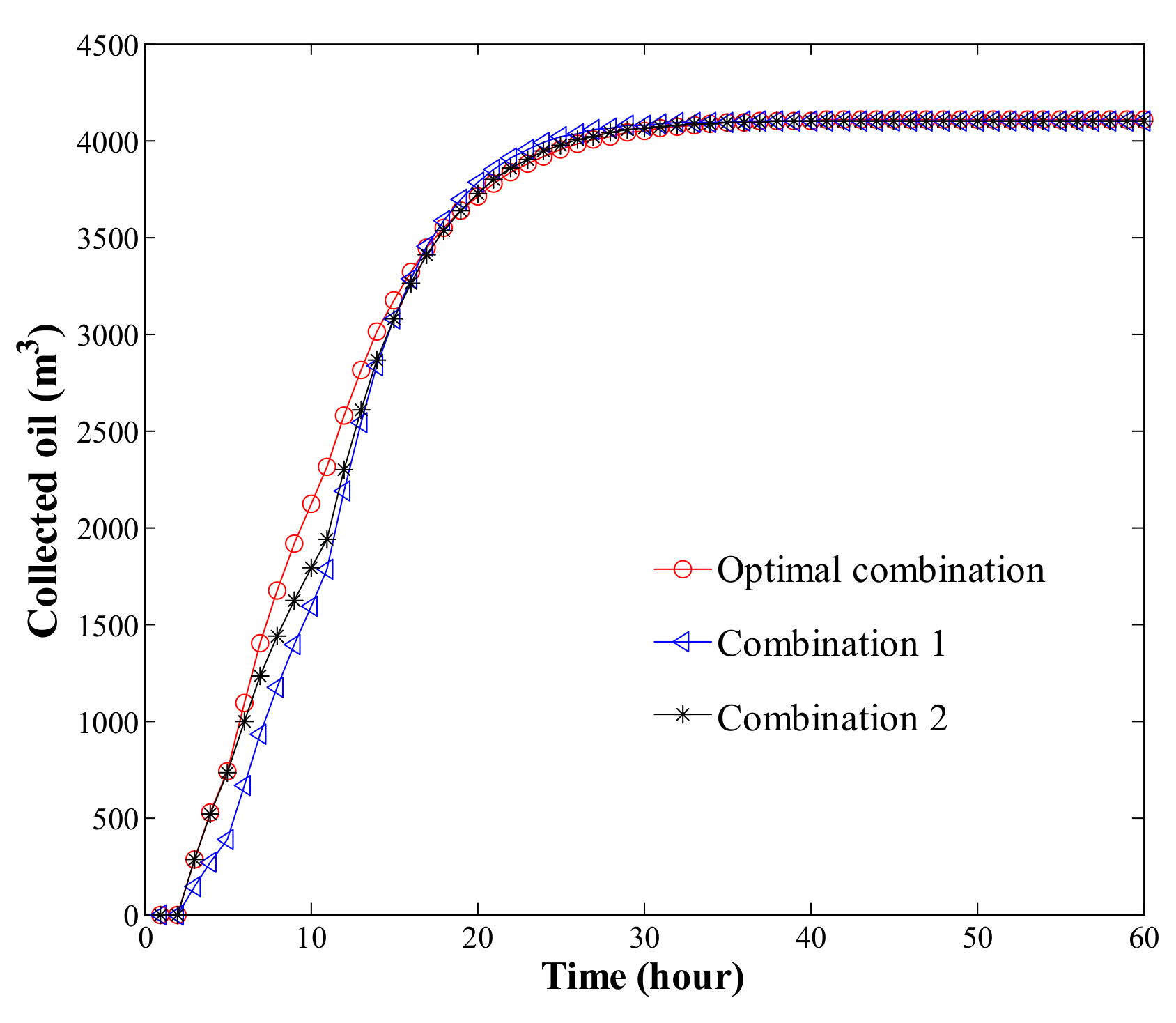
The performance of the optimal skimmer combination {SK₁: eight sets, SK₂: eight sets and SK₃: four sets} was also compared with the combinations of {SK₁: four sets, SK₂: eight sets and SK₃: eight sets} (Combination 1) and {SK₁: eight sets, SK₂: four sets and SK₃: eight sets} (Combination 2). Figure 17 shows the comparisons in oil recovery. Although the oil collection based on the optimal combination (41.0%) was close to the other two combinations’ (40.9%), it appeared to have a significant advantage in the early stage (e.g., the first 15 h). This was of great importance to ecosystem protection because the oil slick was approaching the islands of Saint-Pierre, France and Burin Peninsula, Newfoundland, Canada, about 15 h after the release. The elimination of spilled oil before this time point was urgently needed and the optimal combination was the best one in this case.

4. Conclusions

This study proposed and developed a framework of an integrated decision support system for offshore oil spill management (DSS-OSM). Such a DSS system was developed based on the integration of a Monte Carlo simulation module, a two-stage adaptive resonance theory mapping (TSAM) module, an integrated, rule-based fuzzy adaptive resonance theory mapping (IRFAM) approach and a dynamic, mixed-integer nonlinear programming (DMINP) approach. Accordingly, the DSS-OSM was able to provide effective decision support to offshore oil spill vulnerability index classification, response technology screening and ranking and devices/equipment allocation during response actions.

To demonstrate the feasibility and efficiency of the developed DSS-OSM, a case study regarding decision support to offshore oil spill management was conducted targeting the south coast of Newfoundland, Canada. With the DSS-OSM, a series of decision supports were generated, such as the classified OSVI zones based on different site conditions, a list of ranking scores representing the feasibility of response technologies and the optimal settings of devices/equipment during oil response actions. The modeling result indicated that over 50% of the spill was collected in 12 h, and more than 90% of the oil was removed from sea surface in 1 day. It demonstrated that the proposed DSS was able to provide timely and effective decision support to offshore oil spill management under different environmental and spill conditions. This DSS is also capable of providing decision support to other types of pollution management in offshore and coastal areas.

References

- International Tanker Owners Pollution Federation (ITOPF). Oil Spill Tanker Statistics. 2020. Available online: https://www.itopf.org/knowledge-resources/data-statistics/statistics/ (accessed on 19 December 2021).
- Beyer, J.; Trannum, H.C.; Bakke, T.; Hodson, P.V.; Collier, T.K. Environmental effects of the Deepwater Horizon oil spill: A review. Mar. Pollut. Bull. 2016, 110, 28–51. [Google Scholar] [CrossRef] [PubMed] [Green Version]
- Bursian, S.J.; Alexander, C.R.; Cacela, D.; Cunningham, F.L.; Dean, K.M.; Dorr, B.S.; Ellis, C.K.; Godard-Codding, C.A.; Guglielmo, C.G.; Hanson-Dorr, K.C.; et al. Overview of avian toxicity studies for the Deepwater Horizon natural resource damage assessment. Ecotoxicol. Environ. Saf. 2017, 146, 4–10. [Google Scholar] [CrossRef] [PubMed] [Green Version]
- Echols, B.S. Toxicity evaluation of Louisiana nearshore marsh sediments following the Deepwater Horizon oil spill. Mar. Pollut. Bull. 2021, 168, 112380. [Google Scholar] [CrossRef]
- Griggs, J.W. BP Gulf of Mexico Oil Spill. Energy Law J. 2011, 31, 57–79. [Google Scholar]
- Keramea, P.; Spanoudaki, K.; Zodiatis, G.; Gikas, G.; Sylaios, G. Oil Spill Modeling: A critical review on current trends, perspectives, and challenges. J. Mar. Sci. Eng. 2021, 9, 181. [Google Scholar] [CrossRef]
- Nordvik, A.B. Time window-of-opportunity strategies for oil spill planning and response. Pure Appl. Chem. 1999, 71, 5–16. [Google Scholar] [CrossRef] [Green Version]
- Ye, X.D.; Chen, B.; Lee, K.; Storesund, R.; Zhang, B.Y. An integrated offshore oil spill response decision making approach by human factor analysis and fuzzy preference evaluation. Environ. Pollut. 2020, 262, 114294. [Google Scholar] [CrossRef] [PubMed]
- Shi, X.; Wang, Y.; Luo, M.F.; Zhang, C.J. Assessing the feasibility of marine oil spill contingency plans from an information perspective. Saf. Sci. 2019, 112, 38–47. [Google Scholar] [CrossRef]
- Lazuga, K.; Gucma, L.; Perkovic, M. The model of Optimal Allocation of maritime oil spill combat ships. Sustainability 2018, 10, 2321. [Google Scholar] [CrossRef] [Green Version]
- Grubesic, T.H.; Wei, R.; Nelson, J. Optimizing oil spill cleanup efforts: A tactical approach and evaluation framework. Mar. Pollut. Bull. 2017, 125, 318–329. [Google Scholar] [CrossRef]
- You, F.Q.; Leyffer, S. Mixed-integer dynamic optimization for oil-spill response planning with integration of a dynamic oil weathering model. AIChE J. 2011, 57, 3555–3564. [Google Scholar] [CrossRef]
- Mata, A.; Corchado, J.M.; Tapia, D.I. CROS: A contingency response multi-agent system for Oil Spills situations. Appl. Soft Comput. 2011, 11, 3147–3159. [Google Scholar] [CrossRef] [Green Version]
- Brachner, M.; Stien, F.B.; Hvattum, L.M. A mathematical programming framework for planning an emergency response system in the offshore oil and gas industry. Saf. Sci. 2019, 113, 328–335. [Google Scholar] [CrossRef]
- Pourvakhshouri, S.Z.; Mansor, S.B.; Ibrahim, Z.Z. Oil spill management through a decision support system. Sea Technol. 2006, 47, 53. [Google Scholar]
- Assilzadeh, H.; Mansor, S.; Ibrahim, H. Petroleum hazards management by geomatic systems. In Proceedings of the Asian Conference of Remote Sensing, ACRS2001, Singapore, 5–9 November 2001; pp. 358–363. [Google Scholar]
- Brimicombe, A. GIS, Environmental Modeling and Engineering; Taylor & Francis: London, UK, 2003; p. 378. ISBN 9780429093418. [Google Scholar]
- Leech, M.; Walker, M.; Wiltshire, M.; Tyler, A. OSIS: A windows 3 oil spill information system. In Proceedings of the 16th Arctic Marine Oil Spill Program Technical Seminar, Ottawa, ON, Canada, 7–9 June 1993; pp. 549–572. [Google Scholar]
- Ji, Z.G.; Li, Z.; Johnson, W.; Auad, G. Progress of the oil spill risk analysis (OSRA) model and its Applications. J. Mar. Sci. Eng. 2021, 9, 195. [Google Scholar] [CrossRef]
- Balogun, A.L.; Yekeen, S.T.; Pradhan, B.; Yusof, K.B.W. Oil spill trajectory modelling and environmental vulnerability mapping using GNOME model and GIS. Environ. Pollut. 2021, 268, 115812. [Google Scholar] [CrossRef] [PubMed]
- Yang, Z.Y.; Chen, Z.; Lee, K.; Owens, E.; Boufadel, M.C.; An, C.J.; Taylor, E. Decision support tools for oil spill response (OSR-DSTs): Approaches, challenges, and future research perspectives. Mar. Pollut. Bull. 2021, 167, 112313. [Google Scholar] [CrossRef] [PubMed]
- Fetissov, M.; Aps, R.; Goerlandt, F.; Janes, H.; Kotta, J.; Kujala, P.; Szava-Kovats, R. Next-generation smart response web (NG-SRW): An operational spatial decision support system for maritime oil spill emergency response in the gulf of Finland (Baltic Sea). Sustainability 2021, 13, 6585. [Google Scholar] [CrossRef]
- Amir-Heidari, P.; Arneborg, L.; Lindgren, J.F.; Lindhe, A.; Rosen, L.; Raie, M.; Axell, L.; Hassellov, I.M. A state-of-the-art model for spatial and stochastic oil spill risk assessment: A case study of oil spill from a shipwreck. Environ. Int. 2019, 126, 309–320. [Google Scholar] [CrossRef] [PubMed]
- Nelson, J.R.; Grubesic, T.H. Oil spill modeling: Mapping the knowledge domain. Prog. Phys. Geogr. Environ. 2020, 44, 120–136. [Google Scholar] [CrossRef]
- Gundlach, E.; Hayes, M. Vulnerability of coastal environments to oil spill impacts. Mar. Technol. Soc. J. 1978, 12, 18–27. [Google Scholar]
- Monteiro, C.B.; Oleinik, P.H.; Leal, T.F.; Marques, W.C.; Nicolodi, J.L.; Lopes, B. Integrated environmental vulnerability to oil spills in sensitive areas. Environ. Pollut. 2020, 267, 115238. [Google Scholar] [CrossRef] [PubMed]
- Cai, L.; Yan, L.; Ni, J.L.; Wang, C. Assessment of Ecological Vulnerability under Oil Spill Stress. Sustainability 2015, 7, 13073–13084. [Google Scholar] [CrossRef] [Green Version]
- Azevedo, A.; Fortunato, A.B.; Epifanio, B.; den Boer, S.; Oliveira, E.R.; Alves, F.L.; de Jesus, G.; Gomes, J.L.; Oliveira, A. An oil risk management system based on high-resolution hazard and vulnerability calculations. Ocean Coast. Manag. 2017, 136, 1–18. [Google Scholar] [CrossRef] [Green Version]
- Ertekin, S.; Rudin, C. On equivalence relationships between C=classification and ranking algorithms. J. Mach. Learn. Res. 2011, 12, 2905–2929. [Google Scholar]
- Li, P.; Chen, B.; Li, Z.; Zheng, X.; Wu, H.; Jing, L.; Lee, K. A Monte Carlo simulation based two-stage adaptive resonance theory mapping approach for offshore oil spill vulnerability index classification. Mar. Pollut. Bull. 2014, 86, 434–442. [Google Scholar] [CrossRef] [PubMed]
- Li, P.; Chen, B.; Husain, T. IRFAM: Integrated rule-based fuzzy adaptive resonance theory mapping system for watershed modeling. J. Hydrol. Eng. 2011, 16, 21–32. [Google Scholar] [CrossRef]
- Chen, B.; Li, P.; Husain, T. Development of an integrated adaptive resonance theory mapping classification system for supporting watershed hydrological modeling. J. Hydrol. Eng. 2012, 17, 679–693. [Google Scholar] [CrossRef]
- Li, P.; Chen, B.; Zhang, B. An integrated rule-based adaptive resonance theory mapping approach for technologies screening in offshore oil spill response. In Proceedings of the CSCE 2013 Annual General Conferce, Québec, QC, Canada, 29 May–1 June 2013. [Google Scholar]
- Arbib, M.A. The Handbook of Brian Theory and Neural Networks, 2nd ed.; MIT Press: Cambridge, MA, USA, 2002; pp. 87–90. ISBN 9780262511025. [Google Scholar]
- Price, J.M.; Johnson, W.R.; Marshall, C.F.; Ji, Z.G.; Rainey, G.B. Overview of the oil spill risk analysis (OSRA) model for environmental impact assessment. Spill Sci. Technol. Bull. 2003, 8, 529–533. [Google Scholar] [CrossRef]
- Li, P.; Chen, B.; Zhang, B.Y.; Jing, L.; Zheng, J.S. Monte Carlo simulation-based dynamic mixed integer nonlinear programming for supporting oil recovery and devices allocation during offshore oil spill responses. Ocean Coast. Manag. 2014, 89, 58–70. [Google Scholar] [CrossRef]
- Li, P.; Chen, B.; Li, Z.L.; Jing, L. ASOC: A novel agent-based simulation-optimization coupling approach-algorithm and application in offshore oil spill responses. J. Environ. Inform. 2016, 28, 90–100. [Google Scholar] [CrossRef]
- Fisheries and Oceans Canada. The Grand Banks of Newfoundland: Atlas of Human Activities. 2007. Available online: https://www.dfo-mpo.gc.ca/oceans/publications/nfld-atlas-tnl/page07-eng.html (accessed on 19 December 2021).
- Nazir, M.; Khan, F.; Arnyotte, P.; Sadiq, R. Multimedia fate of oil spills in a marine environment-An integrated modelling approach. Process Saf. Environ. Prot. 2008, 86, 141–148. [Google Scholar] [CrossRef] [Green Version]
- Shen, H.; Yapa, P.; Petroski, M. A simulation model for oil slick transport in lakes. Water Resour. Res. 1987, 23, 1949–1957. [Google Scholar] [CrossRef]
- Wang, S.D.; Shen, Y.M.; Zheng, Y.H. Two-dimensional numerical simulation for transport and fate of oil spills in seas. Ocean Eng. 2005, 32, 1556–1571. [Google Scholar] [CrossRef]
- Al-Rabeh, A.H.; Cekirge, H.M.; Gunay, N. A stochastic simulation model of oil spill fate and transport. Appl. Math. Model. 1989, 13, 322–329. [Google Scholar] [CrossRef]
- Al-Rabeh, A.; Cekirge, H.; Gunay, N. Modeling the fate and transport of Al-Ahmadi Oil Spill. Water Air Soil Pollut. 1992, 65, 257–279. [Google Scholar] [CrossRef]
- Chao, X.B.; Shankar, N.J.; Cheong, H.F. Two- and three-dimensional oil spill model for coastal waters. Ocean Eng. 2001, 28, 1557–1573. [Google Scholar] [CrossRef]
- Chao, X.B.; Shankar, N.J.; Wang, S.S.Y. Development and application of oil spill model for Singapore coastal waters. J. Hydraul. Eng. 2003, 129, 495–503. [Google Scholar] [CrossRef]
- International Association of Oil and Gas Products (IOGP). Coordinatea Conversation and Transformation including Fomulas. 2021, IOGP Report 373-07-2. Available online: https://epsg.org/guidance-notes.html (accessed on 19 December 2021).
- Sarhadizadeh, E.; Hejazi, K. Eulerian oil spills model using finite-volume method with moving boundary and wet-dry fronts. Model. Simul. Eng. 2012, 2012, 7. [Google Scholar] [CrossRef]
Figure 1.
Framework of the MC-TSAM approach (adopt from Li et al. (2014) [31]).
Figure 2.
Framework of the IRFAM approach (adopt from Li et al. (2011) [32]).
Figure 3.
Framework of the MC-IRFAM approach.
Figure 4.
Framework of the MC-DMINP approach (adopt from Li et al. (2014) [37]).
Figure 5.
Framework of the DSS-OSM.
Figure 6.
The movement of spilled oil in 60 h.
Figure 7.
The membership functions of (a) seawater temperature, (b) wave energy/height, (c) wind speed, (d) oil viscosity and (e) slick thickness.
Figure 8.
Skimmer combinations from MC-DMINP results.
Figure 9.
Spill trajectory and volume change based on optimal skimmer combination.
Figure 10.
Simulation results of skimmer ORRn.
Figure 11.
Simulation results of oil viscosity and density, as well as slick thickness.
Figure 12.
Simulation results of oil collection, evaporation and dispersion processes.
Figure 13.
Changes of skimmer combination regarding the uncertainty of slick area.
Figure 14.
Changes of skimmer combination regarding the uncertainty of wind speed.
Figure 15.
Changes of skimmer combination regarding the uncertainty of seawater temperature.
Figure 16.
Correlations between oil budgets (collection, evaporation and dispersion) and uncertain parameters (slick area, seawater temperature and wind speed).
Figure 17.
Performance of skimmer combination in oil collection.