
Phytoplankton Pigments Reveal Size Structure and Interannual Variability of the Coastal Phytoplankton Community (Adriatic Sea)


National Institute of Biology, Marine Biology Station Piran, Fornače 41, SI-6330 Piran, Slovenia
*
Author to whom correspondence should be addressed.
†
The first two authors contributed equally.
Water 2022, 14(1), 23; https://doi.org/10.3390/w14010023
Submission received: 21 September 2021
/
Revised: 14 December 2021
/
Accepted: 20 December 2021
/
Published: 22 December 2021
(This article belongs to the Special Issue Phytoplankton Ecology and Physiology of Coastal Seas)
Abstract
:In coastal seas, a variety of environmental variables characterise the average annual pattern of the physico-chemical environment and influence the temporal and spatial variations of phytoplankton communities. The aim of this study was to track the annual and interannual variability of phytoplankton biomass in different size classes in the Gulf of Trieste (Adriatic Sea) using phytoplankton pigments. The seasonal pattern of phytoplankton size classes showed a co-dominance of the nano and micro fractions during the spring peak and a predominance of the latter during the autumn peak. The highest picoplankton values occurred during the periods with the lowest total phytoplankton biomass, with chlorophytes dominating during the colder months and cyanobacteria during the summer. The highest number of significant correlations was found between phytoplankton taxa and size classes and temperature, nitrate and nitrite. The most obvious trend observed over the time series was an increase in picoplankton in all water layers, with the most significant trend in the bottom layer. Nano- and microplankton showed greater variation in biomass, with a decrease in nanoplankton biomass in 2011 and 2012 and negative trend in microplankton biomass in the bottom layer. These results suggest that changes in trophic relationships in the pelagic food web may also have implications for biogeochemical processes in the coastal sea.
1. Introduction
The size of phytoplankton cells plays an important role in phytoplankton physiology and has major implications for the ecology and biogeochemistry of aquatic ecosystems [1]. There are more than 5000 species of phytoplankton in the world’s oceans [2,3], most of them are in the size range of 1 µm–70 µm range, with some representatives as large as 1 mm [4]. Several abiotic and biotic factors, such as light, nutrient supply, water column stratification and turbulence, water temperature, salinity, grazing, viral infection, etc., influence the growth [5] and cell size distribution [1] of these mostly unicellular algae.
Representatives of different phytoplankton groups differ greatly in terms of morphological, physiological and ecological characteristics. Based on cell size, phytoplankton can be divided into three main size classes: microplankton (20–200 µm), nanoplankton (2–20 µm) and picoplankton (0.2–2 µm) [6]. In the recent rapid development of trait-based ecological studies, body or cell size is among the functional traits that regulate competitive ability (e.g., nutrient uptake rates, growth rates) [7]. Therefore, three size classes are referred to as phytoplankton functional types (PFTs), which have a specific function in an ecosystem [8].
Traditionally, cell dimensions and inferred biovolume and biomass are measured under the microscope, in parallel with taxonomic identification and enumeration. However, microscopy is less suitable for studying the size structure of phytoplankton because it is time consuming and most representatives of the picoplankton size class are hard to observe under a light microscope using the Utermöhl method. Other methods and tools can efficiently complement microscopy, such as High Performance Liquid Chromatography (HPLC), to characterize pigments as chemical markers for phytoplankton groups [9,10], successive filtration to estimate Chlorophyll a (Chl a) in three size classes, flow cytometry to characterize cells based on autofluorescence and light scattering properties, automated cell imaging techniques, and molecular methods, and gene sequencing approaches to characterize diversity. The optical properties of phytoplankton pigments are also studied using ocean colour observations; these have the advantage of high temporal resolution and spatial coverage to provide near real-time data on total Chl a biomass as well as on various PFTs (e.g., [11,12]).
In our study, we used phytoplankton pigments (carotenoids and chlorophylls) as taxonomic biomarkers [9,10] to determine the taxonomic and size structure of field samples. With reference to previous studies [10,13,14], the so-called “pigment indices” were developed with the aim of quantifying the taxonomic composition of phytoplankton as well as size classes using a minimal set of pigments. Seven major pigments were selected to represent different phytoplankton groups (Table 1). These pigment biomarkers can be used to assess the contribution of the three phytoplankton size classes to Chl a concentration [14,15,16]. Cyanobacteria (Zea) and chlorophytes (Chl b) are associated with picoplankton; haptophytes (Hex), dictyochophytes (But) and cryptophytes (Allo) are associated with nanoplankton; and diatoms (Fuc) and dinoflagellates (Per) are associated with microplankton [14,15]. Previous studies [14,16] have already acknowledged that such pigment grouping does not accurately reflect the true size structure of phytoplankton, as different taxonomic groups may share the same biomarker pigments while some groups may occupy more than one size class. Nevertheless, this approach provides a reasonable taxonomic composition of phytoplankton and its size structure [17] and allows determining PFTs with less effort [18] as compared to microscopy. For the northern Adriatic, Terzić [19] showed that seven biomarker pigments explain more than 90% of total chlorophyll biomass.
The aim of this study was to follow the annual and interannual variability of phytoplankton biomass in different size classes in coastal seas (Gulf of Trieste, Adriatic Sea) using phytoplankton pigments as fingerprints of specific groups. The study provides valuable information not only on the taxonomic aspect, but also on the size structure of the phytoplankton community, covering all size classes using the same procedure. This includes picoplankton, which is usually determined separately from nano- and microplankton, but can represent a significant proportion of total phytoplankton biomass in different areas of the northern Adriatic [21,22,23]. Using size-related PFTs over the time series (2007–2018), we then attempted to detect changes in the size structure of the phytoplankton community and associate them with environmental conditions in the Gulf of Trieste.
2. Materials and Methods
2.1. Study Area
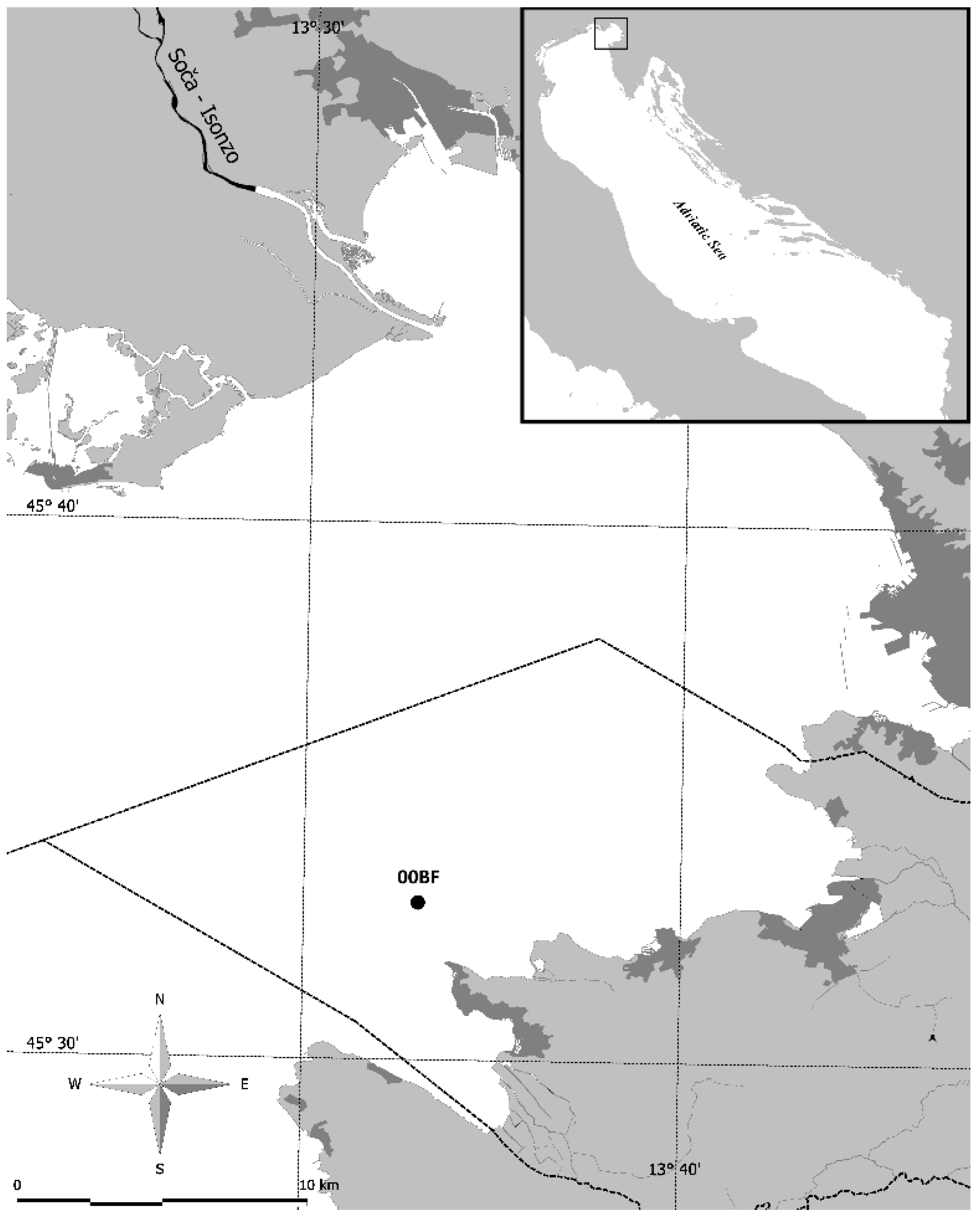
Our study was conducted in the Gulf of Trieste (Adriatic Sea), a semi-enclosed bay with a maximum depth of 25 m (Figure 1), where meteorological conditions, river runoff, prevailing currents and exchange of water masses with the northern Adriatic shape the physical and chemical properties [24]. The nutrient concentration in seawater is strongly modulated by river inflows [25], with the Soča River being the main source [26,27].
Due to the shallowness and closed nature of the Gulf, as well as the high nutrient concentrations, phytoplankton blooms and periods of hypoxia and anoxia were frequently observed in the Gulf of Trieste in the past (from the 1970s to the 1990s) [27,28]. However, an important regime shift was observed in the 2000s, with concomitant changes in some environmental drivers (reduction of river flow and nutrient concentrations) and phytoplankton characteristics (reduction of chlorophyll biomass and seasonal diatom blooms) [29,30].
Apart from high interannual variability, the phytoplankton community of the Gulf of Trieste manifest also a conspicuous annual variability, with biomass peaks in late spring and autumn [31]. The relative contribution of nanoflagellates in terms of abundance to these peaks is higher in spring, while that of diatoms in autumn [31]. Given the trend of decreasing cell size in the oceans due to climate change (increasing stratification) [32], this is also expected in our case, because of perceived long-term changes in temperature and nutrients in the northern Adriatic [33]. However, pigment composition or total biomass (Chl a) alone do not provide information about this process. Therefore, biomass in different size classes was investigated.
2.2. Field Sampling and Measurements
Seawater was sampled in the south-eastern part of the Gulf of Trieste at offshore sampling site 00BF (1.3 nautical miles offshore, depth 22 m, 45°32,928′ N, 13°33,032′ E; Figure 1). Seawater samples for phytoplankton pigments and nutrients were collected every two weeks, from January 2007 to December 2018 using Niskin bottles (5 L) at 1 m, 10 m and 21 m depths.
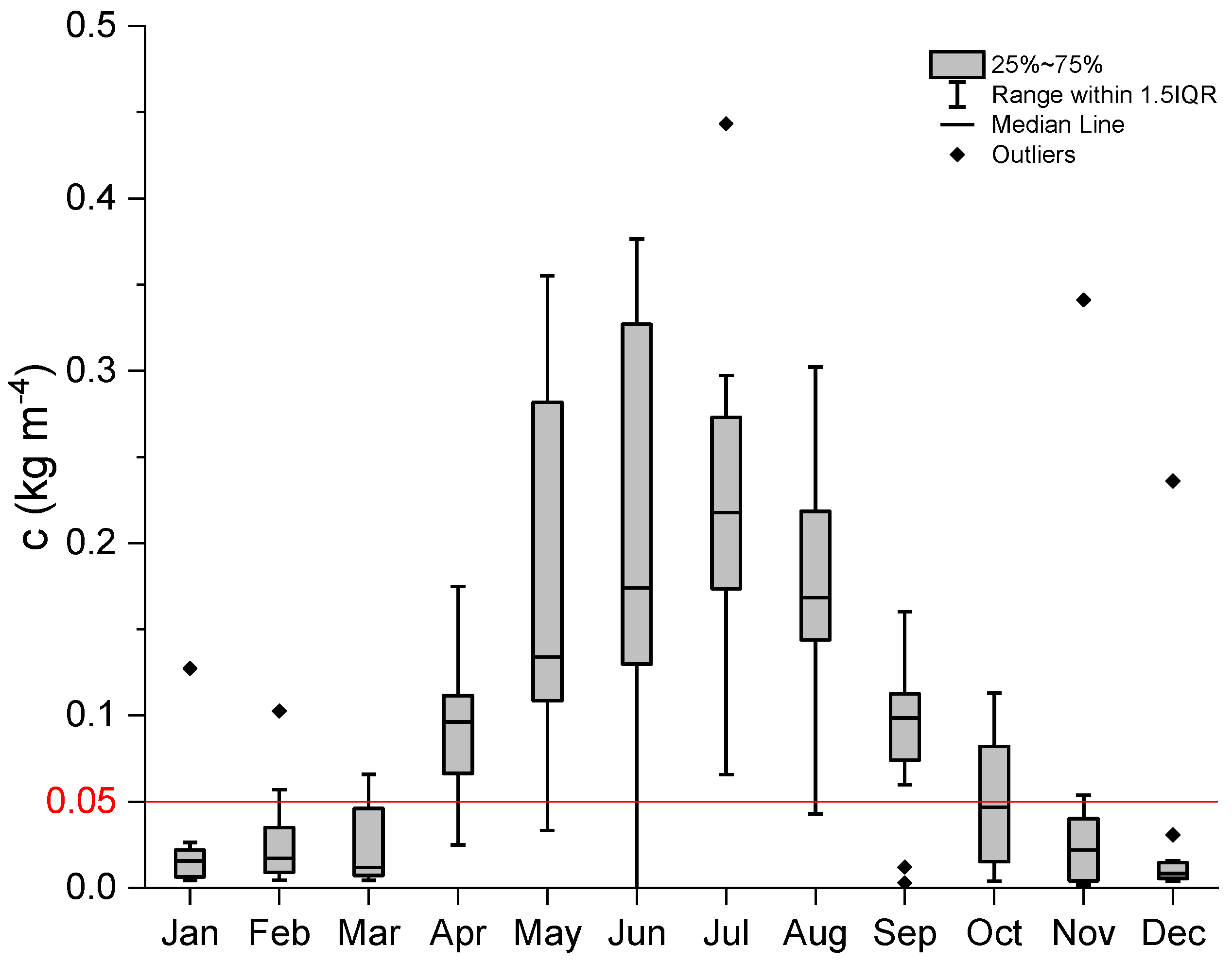
Vertical profiles of temperature, salinity and density were obtained using a fine scale CTD probe (Conductivity Temperature Depth; Sea & Sun Technology GmbH, Trappenkamp, Germany). The bulk density gradient (c) calculated from the bottom and surface density was used as an indicator of stratification: if c < 0.05 kg m−4 mixed water column, if c > 0.05 kg m−4 stratified water column.
In the 12-year time series, 2007–2018, two periods were considered in the subsequent analysis of the data:
Period 2007–2014, to show the average annual dynamics of physical and chemical variables, as well as the taxonomic and size structure of phytoplankton;
- -
- Period 2007–2018, to identify trends in phytoplankton biomass and size structure.
- -
- The reason for this is that the method used for analysing nutrients changed in 2015.
2.3. Laboratory Analyses
Concentrations of inorganic nutrients (nitrate—NO3−, nitrite—NO2−, ammonium—NH4+, ortophosphate—PO43− and silicate—SiO44−) were measured in unfiltered samples using standard colorimetric methods [34] and their modifications [35].
Phytoplankton pigments, including Chl a, were determined by a reversed phase High Performance Liquid Chromatography (HPLC) method [36,37]. Water samples (1 L) were filtered through 47 mm Whatman GF/F filters and frozen immediately (at −80 °C) until analyses. Frozen samples were extracted in 4 mL of 90% acetone (for liquid chromatography, LiChrosolv®, Merck KGaA, Darmstadt, Germany) by sonication, and centrifuged at 4000 rpm for 10 min to remove particulates. A mixture (1:1) of clarified extract and 1 mol L−1 ammonium acetate (pro analysis, Merck) was injected into a gradient HPLC system (1260 Infinity, Agilent Technologies, Santa Clara, CA, USA) with a 200 µL loop. The HPLC system was equipped with a reversed phase 3 µm C18 column (Pecosphere, 35 × 4.5 mm, Perkin Elmer, Shelton, CT, USA). Chlorophylls and carotenoids were detected by absorbance at 440 nm using a DAD (Agilent Technologies, model 1290 Infinity). Data acquisition and integration were performed using Agilent ChemStation A 10.02 software. Further down, phytoplankton pigments are referred to abbreviations, as in Table 1.
To calculate the different size classes of phytoplankton as a fraction of total biomass (f), the equations developed by Claustre [15], Vidussi et al. [14], and Uitz et al. [16] were used:
where wDP represents the weighted sum of the concentrations of seven diagnostic pigments:
fmicro = (1.2[Fuc] + 1.5[Per])/wDP
fnano = (1.85[Allo] + 1.6[But] + 1.1[Hex])/wDP
fpico = (1.7[Zea + Lut] + 0.9[Chl b])/wDP
wDP = 1.2[Fuc] + 1.5[Per] + 1.85[Allo] + 1.6[But] + 1.1[Hex] + 1.7[Zea + Lut] + 0.9[Chl b]
The concentrations of each biomarker pigment are multiplied by the published values of coefficient K (average ratio between the concentration of Chl a and the biomarker pigment; Table 1) to account for the natural variability in the contribution of each pigment to the biomass of different phytoplankton groups. It should be noted that in this work both Zea and Lut were used to detect cyanobacteria because the method does not separate these two pigments.
The concentration of Chl a associated with each phytoplankton size class was then calculated as:
where fmicro + fnano + fpico = 1.
[Chl a]micro = fmicro × [Chl a]
[Chl a]nano = fnano × x [Chl a]
[Chl a]pico = fpico × [Chl a]
The relationships between biological and environmental variables (2007–2014) were evaluated using Spearman’s rank correlation, which does not require any assumptions about distribution [38]. The statistical significance was set at the p < 0.001.
The interannual variability of phytoplankton size classes was determined using time series of phytoplankton pigments (2007–2018) and then calculated as Chl a concentrations for each size class. In total, 1605 samples were analysed. Using the monthly means of these data, linear regression was calculated to determine a temporal trend and analyses of variance were performed to test statistical significance. In order to discern interannual variability of phytoplankton pigments and related taxonomic groups, the Seasonal-Trend decomposition process based on Loess—STL [39] was used. With this method, the long-term trend is separated from the seasonal and remainder component in a time-series of data [39].
3. Results
3.1. Physical and Chemical Characteristics of the Study Site
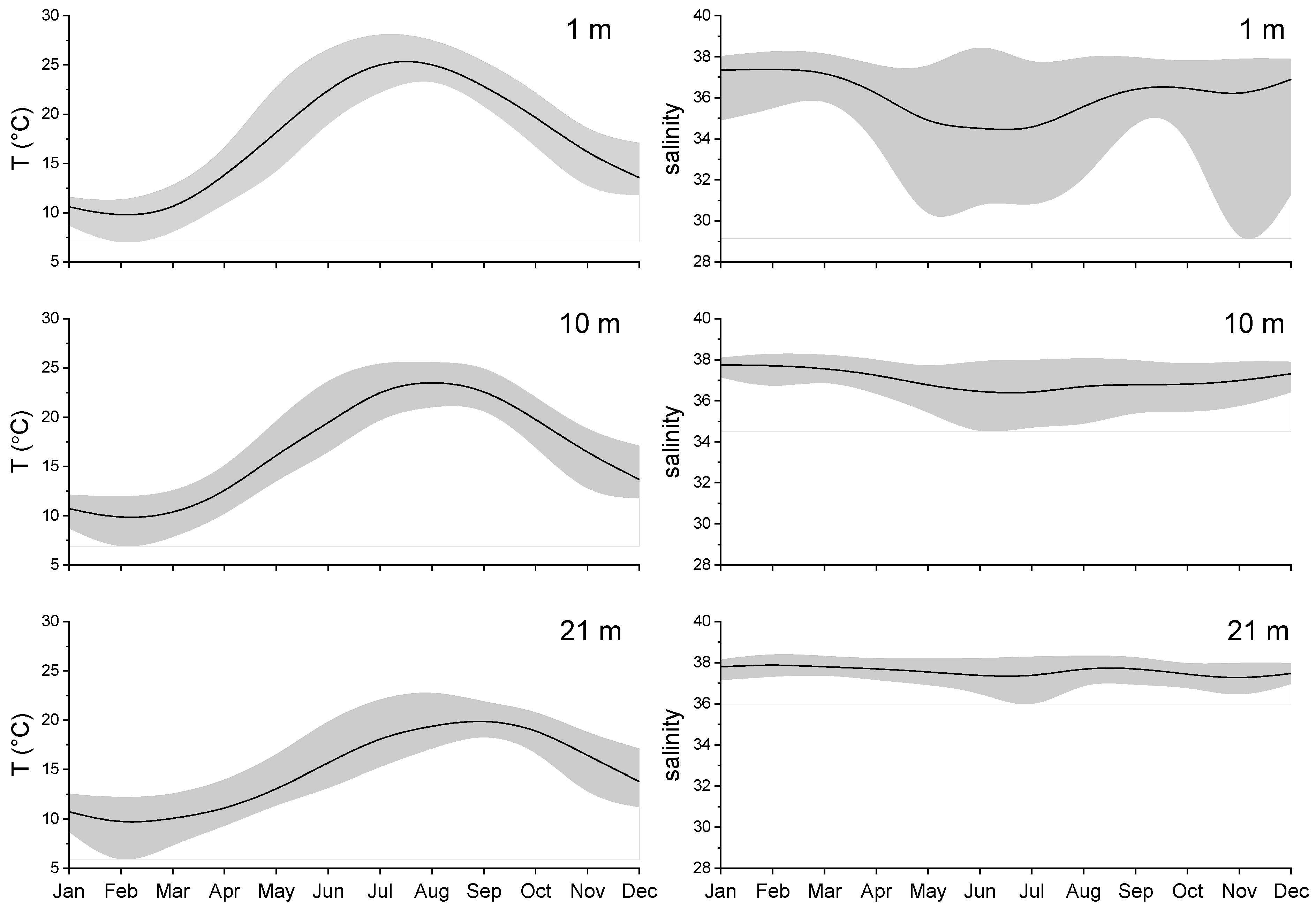
The highly variable environment of the Gulf of Trieste is reflected in wide ranges of environmental variables (Figure 2, Figure 3 and Figure 4). During 2007–2014, water temperature at the surface of the sampling site averaged between 9.5 °C in February and 25.5 °C in August (Figure 2; left panel). In the bottom layer, the temperature range was smaller (between 9.4 and 20.4 °C on average). The lowest temperatures were always measured in February, while the temperature peak in the bottom layer was delayed by one month (September) compared to the upper water layers (August). Large variations in salinity observed in the surface layer indicate the influence of freshwater inputs from rivers and precipitation distributed over late spring/summer and late autumn (Figure 2; right panel). The highest salinities were measured in winter in all three layers (from 37.4 at the surface to 37.9 at the bottom), while the lowest average value was reached in July (34.3 in the surface layer). In the lower layers, variations in salinity were much smaller than in the surface layer. On average, the water column was stratified from April to September, as shown by density gradient values of more than 0.05 kg m−4 (Figure 3). The spring months (May, June) were characterised by high instability due to frequent interruptions in the stratification of the water column.
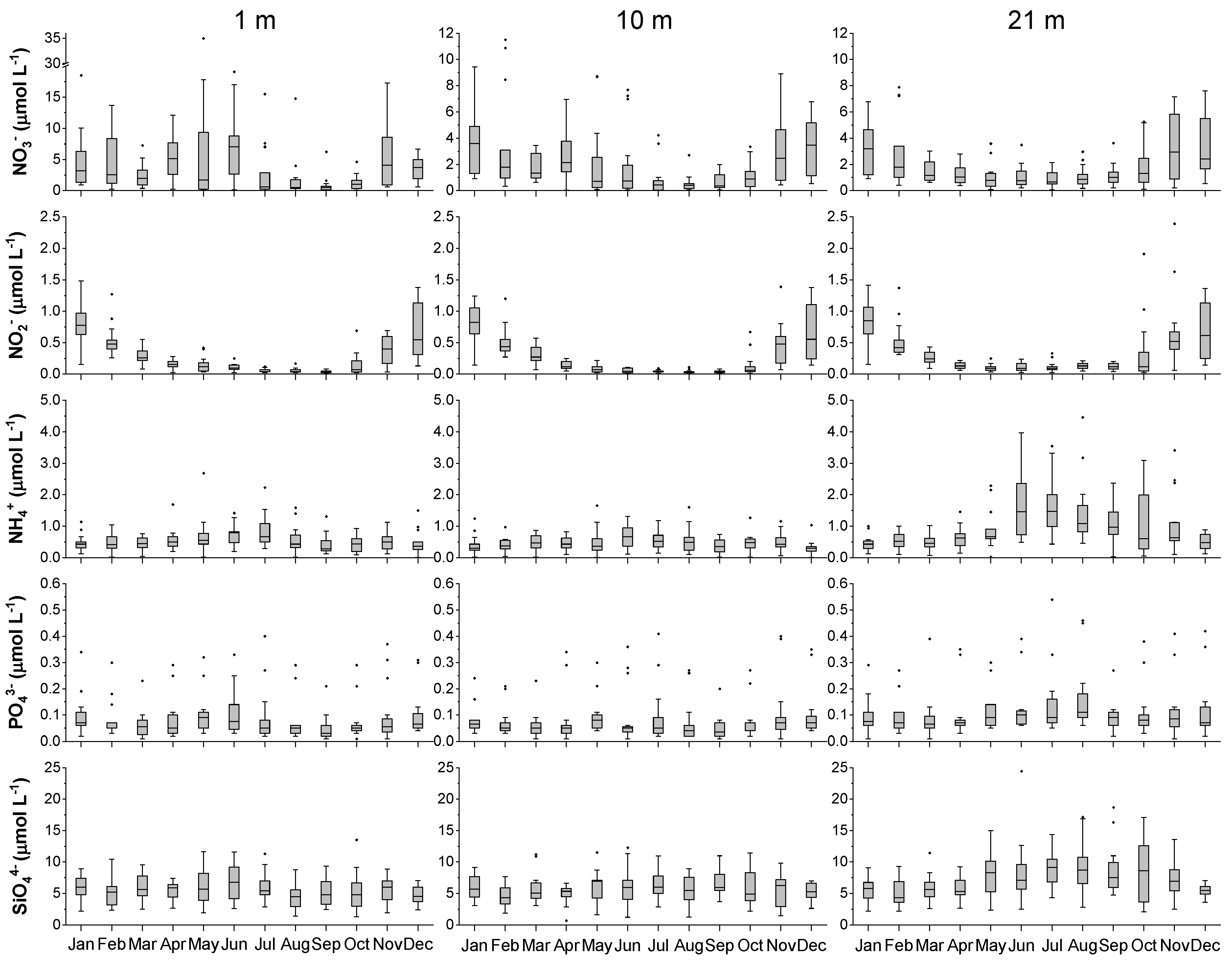
Nutrient concentrations varied considerably during the study period (Figure 4). Several nitrate peaks were observed in the upper 10 m layers in spring and autumn, with maximum concentrations at the surface (35 µmol L−1) being much higher than those in the 10 m layer (11.5 µmol L−1). In the bottom layer, the highest concentrations were measured in late autumn and early winter. A similar seasonal cycle with peak values in the cold months was observed for nitrite in all three layers (highest median 0.85 µmol L−1). Ammonium was characterised by high concentrations in the stratified water column, reaching maximum values in the bottom layer (highest median 1.5 µmol L−1 in July). Ortophosphate concentrations were very low on average, with median values always below 0.1 µmol L−1 and no clear seasonality. The annual pattern of silicate was similar to that of ammonium, reaching the highest concentrations in the bottom layer in the period from May to October (highest median 9.1 µmol L−1 in July).
3.2. Annual Variability of Phytoplankton Size Classes and Taxonomic Groups
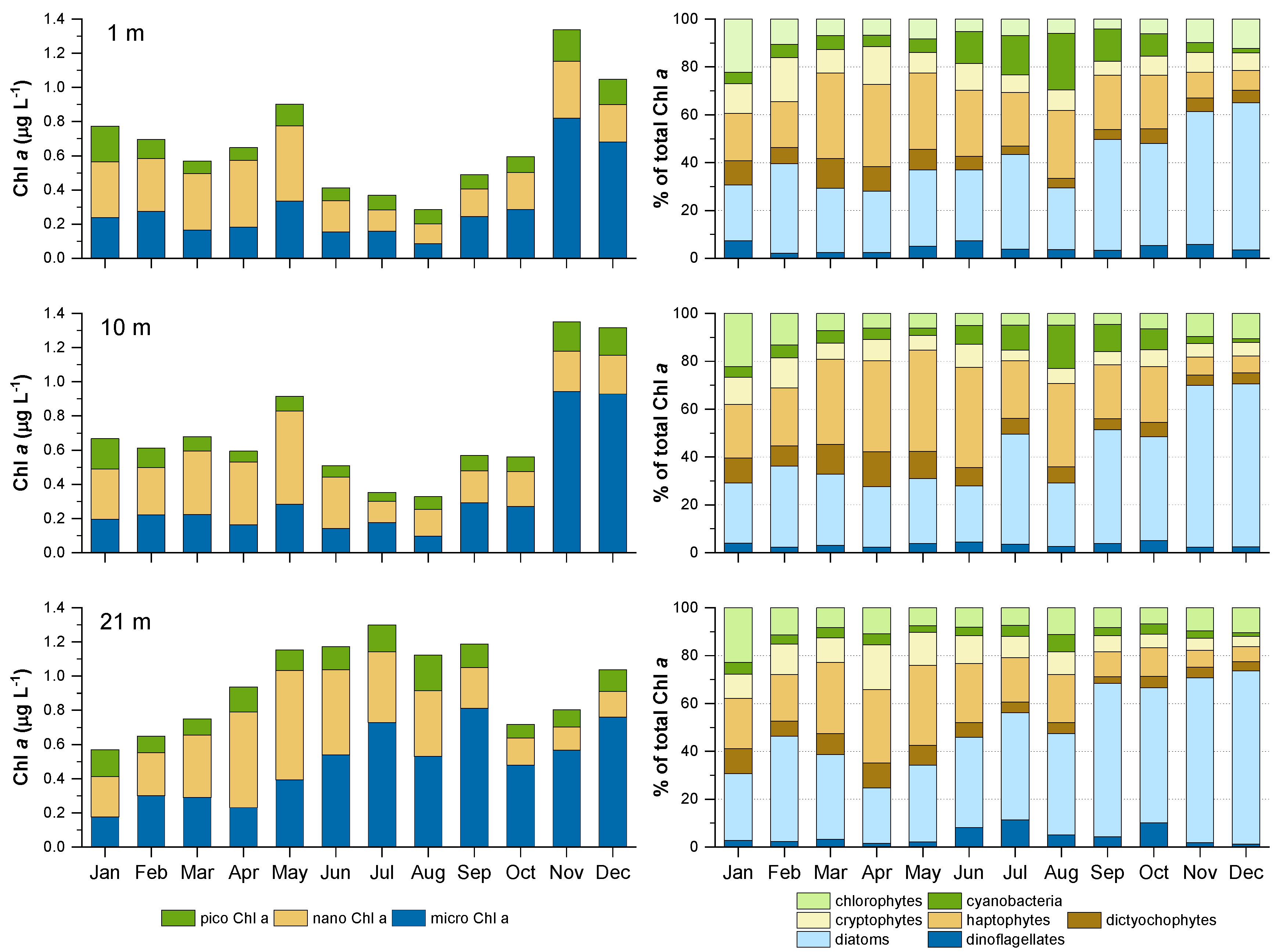
During the 2007–2014 period, Chl a biomass in the 1 and 10 m layer expressed two annual peaks, the first one in May (average 0.9 µg L−1) and second one, more pronounced, in November-December (average 1.3 µg L−1) (Figure 5; left panel). During the autumn peak, the microplankton size class dominated, accounting for up to 70% of biomass while during spring most of the biomass was distributed among nanoplankton (up to 60%) and microplankton (up to 30%, Figure 5; right panel). In the bottom layer, the seasonality of biomass was different, with high Chl a values over the stratified water column period (peak in July 1.3 µg L−1, Figure 5; left panel). Microplankton contributed most to this summer peak (up to 56%), followed by nanoplankton (32%) (Figure 5; right panel). The contribution of picoplankton to Chl a biomass was low over all months in the whole water column, reaching the lowest values during Chl a peaks (about 10%). Conversely, picoplankton made up 30% of phytoplankton biomass during the lowest Chl a concentrations (in August, in the upper 10 m and in January in the entire water column; Figure 5).
Diatoms, which were the dominant group in the microplankton size class, attained the highest share in Chl a biomass during autumn in all three water layers (up to 72%; Figure 5, right panel). The second group of microplankton, dinoflagellates, contributed the least to the biomass, on average; however, the highest contribution was observed in the bottom layer during summer (up to 11%). During spring, the highest contribution to total biomass (up to 42%) was attributed to haptophytes, the dominant group of the nanoplankton size class. Also, the contribution of dictyochophytes to overall biomass was the highest during spring, but did not exceed 15%. The third nano-sized group, the cryptophytes, contributed most during the first half of the year, but never more than 19% of total biomass. The two picoplankton groups alternated their contribution over the year in the upper 10 m layer, with chlorophytes contributing most to phytoplankton biomass during the coldest months (up to 22%) and cyanobacteria during the stratification period (up to 24%). In the bottom layer, the contribution of cyanobacteria was always low.
The correlation with total Chl a was highest for microplankton (r = 0.85–0.86 for the three water layers), although the correlations were significant for all three size classes with p < 0.001 (Table 2). Cyanobacteria were the only group that did not correlate with total Chl a biomass.
Most of the significant correlations (p < 0.001) were found between phytoplankton taxonomic and size groups and temperature, nitrate and nitrite, while there were only a few significant correlations between the other variables (Table 2). In the upper 10 m, the biomass of all three classes of nanoplankton (dictyochophytes, haptophytes and cryptophytes) was negatively affected by temperature. The relationship with temperature was different for the two groups of picoplankton, chlorophytes correlated negatively and cyanobacteria correlated positively with temperature. The correlation between temperature and microplankton biomass was negative in the upper 10 m and was led by the correlation with diatoms. On the contrary, it was positive in the bottom layer for both diatoms and dinoflagellates. Some groups (dinoflagellates and cyanobacteria) showed a negative correlation with salinity, while chlorophytes were positively correlated with this parameter. Most of the groups were positively correlated with nitrate and nitrite in the upper 10 m, except for haptophytes and cyanobacteria, while there were fewer significant correlations at the bottom, and all negative. Only two significant correlations were found for ammonium and silicate, and three for orthophosphate.
3.3. Long-Term Trends of Phytoplankton Biomass and Size Structure
At the annual level, the most consistent changes in the period 2007–2018 were observed for the picoplankton size class (Table 3); the biomass in this size class had increased in all three layers with the most significant trend in the bottom layer. At the same time, biomass in the microplankton size class decreased, but only in the bottom layer.
When considering the seasonal averages, significant trends were observed only in the second part of the year—in summer and autumn (Table 3). During summer, picoplankton biomass increased in the 10 and 21 m layers, while in autumn this trend was also observed in the surface layer. The nanoplankton trends, which were not evident on the annual level, showed an increase in the surface and middle layers during summer and in the bottom layer during autumn. The decrease in microplankton biomass in the bottom layer was the most pronounced during summer, which is also indicative of a negative trend in this layer on an annual level.
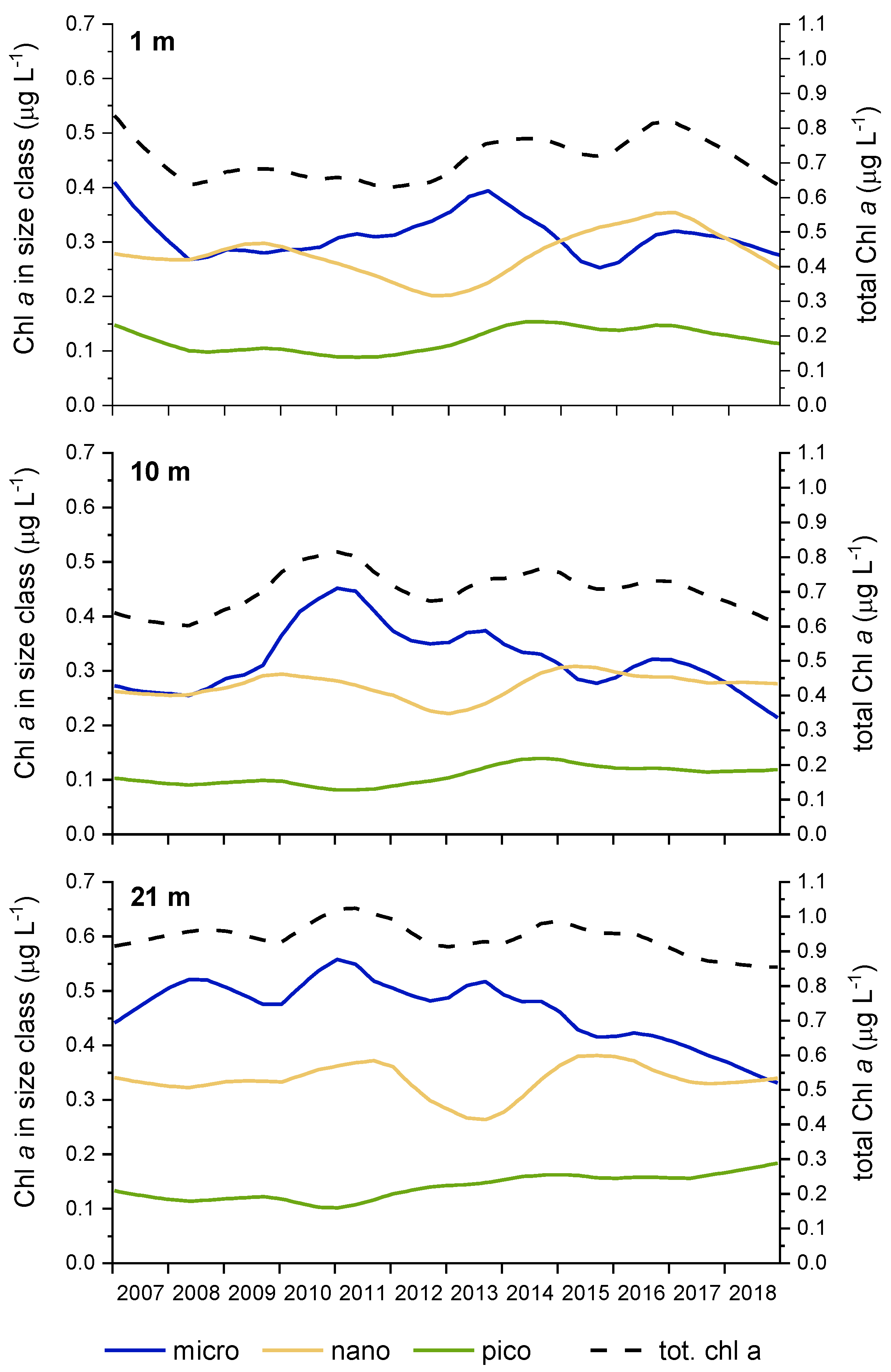
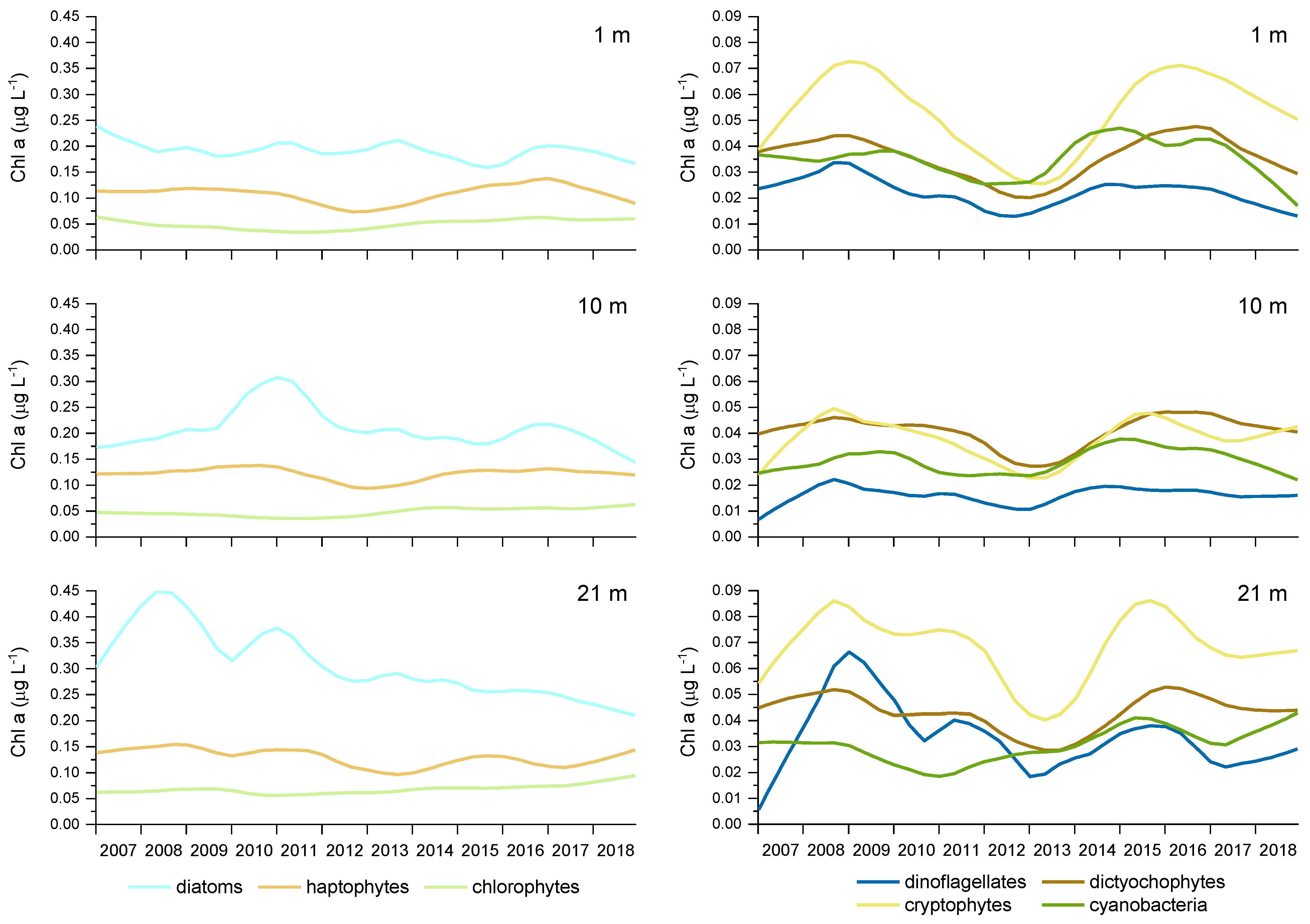
The results of the STL analyses also showed a decrease of Chl a in the microplankton size class (Figure 6), mainly due to diatoms (Figure 7), especially in the bottom layer. On the other hand, an increasing trend of Chl a in the picoplankton size class was observed, mainly due to chlorophytes and cyanobacteria especially at the bottom (Figure 7). An interesting oscillation in Chl a in the nanoplankton size class was also observed, with a decreasing trend in 2011 and 2012. As of 2013, Chl a in the nanoplankton size class increased gradually, reaching similar values to those noted at the beginning of the study (Figure 6). This decrease was due to the lower biomass of haptophytes and cryptophytes (Figure 7).
4. Discussion
Large variations in phytoplankton biomass, taxonomic composition and size are among the most recurring characteristics of the communities in the coastal area of the Gulf of Trieste. This is undoubtedly linked to the dynamics of the pelagic environment in which they live, with large fluctuations in a variety of physical and chemical factors (e.g., [40]). However, the environmental factors that drive these changes in phytoplankton communities are difficult to discern in such a variable system. Past research in the area evidenced the most important influences in the freshwater discharges and general regulation of nutrient sources such as the ban on the use of phosphorus in detergents, and wastewater treatment [27]. For example, dry periods characterized by low freshwater discharge and decreasing orthophosphate concentrations in seawater resulted in a decrease of phytoplankton biomass in the northern Adriatic [41], less intense diatom blooms and an increase in the abundance of flagellated forms of nano-sized phytoplankton in the Gulf of Trieste [29]. The use of phytoplankton pigments as equivalents for certain taxonomic groups and size classes in our study helped to elucidate certain characteristics in the size-structure of small-sized phytoplankton, i.e., nanoplankton and picoplankton, and their recent changes, in line with the observations in many parts of the world’s oceans [1].
The shift towards smaller phytoplankton cells is often linked to climate related changes such as increases in seawater temperatures [1,42]. Warming of the water column has been reported from the northern Adriatic [43] including the Gulf of Trieste [44]. Temperature affects phytoplankton mostly indirectly, through intensified water column stratification and reduced nutrient availability [45] or through enhance top-down control of zooplankton grazers [32,46]. In our study, temperature was negatively related to the biomass of most phytoplankton groups in the upper part of the water column, with the exception of cyanobacteria for which the relationship with temperature was significantly positive. These general positive correlations indicate that, for most of the groups, phytoplankton growth is driven by processes occurring outside the warmest period, and indirectly confirms that it is more connected to other drivers, such as nutrient concentrations. Among these, oxidised nitrogen forms (nitrate and nitrite) displayed most of the positive correlations with phytoplankton groups. Their primary source in the Gulf of Trieste are freshwater inputs, with River Soča (Isonzo) being the most important one, and precipitation [47,48], both of which peak in late winter-early spring and autumn (Source: Hydrological Data Archive of Slovenian Environment Agency). Nitrate and nitrite seem to affect the members of all three size groups, though the growth of nanoplankton was apparently more stimulated in spring when they constituted the majority of biomass. Nitrate is known to be an important driver of spring phytoplankton blooms [47,49]. Ammonium, which was found in high concentrations in the bottom layer throughout summer, is known to fuel autumn phytoplankton blooms after water column mixing [31,50], but these relationships were not evidenced by our analysis. Diatoms might take advantage of this, since they are the dominating phytoplankton group during autumn blooms. However, phytoplankton uptake of excess nitrogen in nutrients is limited by the availability of orthophosphate, known to be the limiting nutrient in the northern Adriatic [31]. As orthophosphate concentrations were very low during our study, the correlations with phytoplankton were not significant. Indeed, phytoplankton biomass in the northern Adriatic is more related to total phosphorus concentrations (data not available for our study) [51] and thus reinforce the importance of rapid recycling of phosphorus for phytoplankton growth [31].
Phytoplankton pigment analysis revealed that Hex was the dominant pigment in the spring period. Based on past work in the Gulf of Trieste [19], Hex was used to track the biomass of haptophytes in this study. However, Hex can also be found in some of dinoflagellates and dictyochopytes species [52]. Similarly, But can be found in some taxa except dictyochophytes, such as haptophytes and pelagophytes [53]. As for the latter group, its representatives occur in various marine environments, from the coast to the open sea [54,55] and have been found to be important in deep waters of the Mediterranean [56] However, their occurrence and distribution in the Adriatic Sea is scarcely described [57]. Allo is the major pigment in cryptophytes and it is rarely reported to be present in other taxa [53,58]. The great majority of taxa in all these groups are nano-sized. Therefore, we infer that the three phytoplankton groups marked by Hex (haptophytes), But (dictyochophytes) and Allo (cryptophytes) jointly represent the nano-sized class in the Gulf of Trieste rather well. Once again, this emphasizes the importance of the nano-sized compartment during the spring period. Nano-sized diatoms can also contribute to the spring peak in the area, e.g., Cyclotella spp. and small Chaetoceros species [41,48,59,60] but, in our study, they were classified in the micro fraction based on pigment signature.
After the breakdown of stratification in autumn, which normally coincides also with increased runoff from the River Soča in October and November [61], phytoplankton biomass reaches its second and highest peak. Unlike the spring one, it is dominated by the micro size class along the entire water column (>60%) and diatoms account for the largest share. In contrast, when abundance was considered, the autumn peak was co-dominated by diatoms and nanoplanktonic flagellates in the same study area and time period [31]. This difference can be attributed, to a great extent, to the small size of nanoflagellates and large diatom blooming during this period [31]; however, it could be partly explained by the non-absolute specificity of pigment biomarkers. For example, many algae that are not diatoms also have high Fuc concentrations [62]. Furthermore, pigment signature can vary on a seasonal basis. Ansotegui et al. [63] found that Fuc occurs mainly in the microplankton size class during the first half of the year and in the nanoplankton size class the rest of the time, when it originates mainly from cryptophytes and haptophytes.
In the bottom layer, phytoplankton biomass and size structure follow a different pattern, which is defined by the shallow depth of the study area that allows sufficient light to reach the bottom, and remineralization of nutrients under stratified water column conditions. High biomass throughout late spring and summer may result from in-situ growth in the bottom layer, sedimentation of cells from the upper layers and their accumulation near the bottom [48,64] and/or photoacclimation processes [65]. The higher contribution of microplankton to phytoplankton biomass in the bottom layer compared to the upper water column was partly attributed to dinoflagellates, especially in June and July. This high contribution of dinoflagellates during summer is typical of the northern Adriatic Sea [21,60,66] and may be linked to their ability to cope with stratified water column conditions by vertical migrations and mixotrophy [67].
The picoplankton size class contributed the least to phytoplankton biomass. However, its importance may not be comparably small, especially during the period of low biomass in summer. For example, cyanobacteria displayed the highest Chlorophyll a-normalized primary production in the Gulf of Trieste [68], and an important contribution of picoplankton to primary production during periods and areas of low primary production has been demonstrated globally [45]. The picoplankton size class is often neglected in phytoplankton studies, since methods other than microscopy are necessary for their evaluation. They are analysed separately from the rest of the phytoplankton community (e.g., studies using flow cytometry such us in Šantić et al. [69], and the results are thus more difficult to compare. In this study, picoplankton biomass in the upper layers was the highest in winter when it was dominated by chlorophytes, which is in agreement with the winter peak of picoeukaryotes in the NE Adriatic [23]. Šilovič et al. [23] also found that Synechococcus, the dominant type of cyanobacteria, was the most abundant at the end of summer and early autumn, which is also similar to our finding, namely, that the contribution of cyanobacteria to picoplankton biomass in the upper water layers is the highest during the summer months. A different seasonality of picoplankton was observed in the nearby Gulf of Venice [21], where picoplankton biomass peaked from summer to autumn but, as with our study, it dominated during periods of lowest total phytoplankton biomass.
Our study also addressed the interannual variability of phytoplankton biomass of different taxa and size classes. The most consistent trend observed in all layers during 2007–2018 was the increase in picoplankton, while in the other two size classes the trend was not as straightforward. For example, the biomass of nanoplankton showed an increase in summer (at 1 and 10 m) and autumn (at 21 m), but when the seasonal component was removed, the trend of nanoplankton showed a sharp decrease during 2011–2012 and subsequent recovery. This depression was observed, based on biomarker pigments, for all three groups (haptophytes, cryptophytes and dictyochophytes) forming the nano size class in all layers and for dinoflagellates. The same nanoplankton decrease was observed with phytoplankton abundance studies in the Gulf of Trieste [59,60]. The nano-sized phytoplankton is top-down controlled mainly by the microzooplankton [70], which is very efficient in this area [71], and could play a role in the short-term oscillation of nanoplankton. For example, Monti et al. [72] found that in the Gulf of Trieste, there was a sharp decline in tintinnids (which constitute a part of the microzooplankton community) between 1998 and 2010 compared to the previous period, but they started to recover gradually after 2007 [73]. This trend for tintinnids was the opposite of that for nano-sized flagellates, that increased in abundance in 2003–2009 compared to 1989–2002 [29], and was related to the combined effect of oligotrophication and grazing control in the Gulf of Trieste.
Moreover, the decrease in diatom abundance peaks in 2003–2009 was attributed to the oligotrophication process [29]. The interannual variability of microplankton during our study, mainly determined by the trend of diatoms (Fuc), and especially the decrease of microplankton biomass in the bottom layer could indicate the continuation of severe phosphorus limitation, observed in the northern Adriatic as a consequence of changes in riverine discharges and anthropogenic phosphorus loads [33]. Moreover, the deseasonalized trends of micro- and nanoplankton had approximately an opposite direction, e.g., in 2012–2014 and 2016, which could indicate that both size classes are at least partly modulated by the same bottom-up processes that drive the phytoplankton community towards prevalence of small-sized taxa [45]. The highest share of small-sized taxa in relation to a reduced pool of nutrients could indicate both a switch towards nanoplanktonic flagellates and towards smaller diatom species. From this point of view, the upward trend of diatom biomass in spring could be part of the same process, considering that Fuc also characterizes nano-sized diatoms.
The upward trend in picoplankton during 2007–2018 was significant in all three water layers, but was most pronounced near the bottom. This trend was mainly driven by the trend of chlorophytes (Chl b) as it represents the major part of picoplankton biomass. However, the concentrations of cyanobacteria (Zea+Lut) were also higher in the second half of the time series than in the first. Although both picoplankton groups showed a positive trend in biomass over time, the mechanism behind this process is probably different. Cyanobacteria and chlorophytes exhibited different seasonality and an opposite relationship with some of the driving factors. The correlation between cyanobacteria biomass and temperature was positive and between salinity negative. The same has been observed for the dominant cyanobacteria Synechococcus in the NE Adriatic Sea [23]. Cyanobacteria have a competitive advantage at higher temperatures [74] and models predict an increase of both Prochlorococcus and Synechococcus with increasing temperature in the world’s oceans [75]. This advantage could be one of the reasons for the observed trend in our study. It has been reported that Prochlorococcus type cyanobacteria may also benefit from increasing oligotrophication [76]. Prochlorococcus has been found to constitute a small part of cyanobacterial biomass in the central and southern Adriatic and is mainly present during the colder seasons [69,77] However, to our knowledge, Prochlorococcus has not yet been determined in the northern Adriatic while Synechococcus represents an important part of picoplankon in this area [22,40]. Paoli et al. [22] suggested that heterotrophy is an important additional trait that supports the success of Synecchococcus in the Adriatic Sea and supported a rise in the abundances of this organism observed over 1993–2004 [78].
Contrarily to cyanobacteria, the environmental preferences of chlorophytes and their tendency to accumulate in the bottom layer during stratified water column conditions may indicate that the driver for the upward trend of chlorophytes is more related to the availability of nutrients and water column conditions rather than temperature. Indeed, chlorophyte biomass was negatively or not correlated with temperature during our study, but showed a strong positive correlation with nitrate and nitrite. Picoeukaryotic plankton (that at least partly can be paralleled to chlorophytes in our case) displayed similar behaviour in other parts of the Adriatic Sea [23,69]. A higher contribution of picoplankton to the overall biomass of phytoplankton could change the balance between the classical food chain channelling energy towards higher trophic levels and the microbial loop, which is less efficient in carbon cycling [1,79]. Moreover, the share that picoplankton biomass occupy in phytoplankton community as calculated in our study may be underestimated, as it was based only on chlorophytes and cyanobacteria as assessed by pigments Chl b and Zea+Lut, respectively. Taxa belonging to other groups, e.g., haptophytes, chrysophytes and pelagophytes have members in the pico compartment as well [79]. Further investigations in the Gulf of Trieste should be carried out to reveal the detailed composition and dynamics of the picoplankton size class and to confirm the presence of Prochlorococcus, using flow cytometry and/or molecular methods.
5. Conclusions
In this study, we show that the results of HPLC analyses, i.e., concentrations of biomarker pigments, can also be used to determine the chlorophyll biomass in three phytoplankton size classes. Two important pieces of ecological information can be obtained from a single analysis (HPLC)—the coarse taxonomic structure and the size structure of the phytoplankton community.
Our long-term analyses have shown that the biomass of phytoplankton groups, partitioned into three size classes, generally parallels the seasonality of abundance with two annual peaks, as demonstrated in previous studies in the area. In terms of size, there is an alternation of dominance between the spring peak, where nano- and microplankton jointly account for a substantial share of total biomass, and the autumn peak, where microplankton (mainly diatoms) account for most of the biomass. The biomass of picoplankton, which consists mainly of chlorophytes, is highest in the colder months, while cyanobacteria play a greater role in summer.
The most obvious trend observed during 2007–2018 was an increase of picoplankton in all water layers, which may be due to several factors, such as increasing water temperatures, intensified stratification during summer and nutrient availability. The other two size classes showed more fluctuating biomass over the time series, with a sharp decrease in nanoplankton biomass in 2011–2012, which was also observed in other studies in the Gulf of Trieste.
For the Gulf of Trieste, where picoplankton is not routinely monitored, our study provides a first insight into the temporal distribution of picoplankton in relation to other size groups, and allows drawing important ecological conclusions. For example, the increase in picoplankton biomass, together with changes in the proportion of phytoplankton size classes, could have significant implications for trophic relationships in food web and the fate of carbon in the coastal sea.
Author Contributions
Conceptualization, P.M., V.F.-P. and J.F.; methodology, V.F.-P., P.M. and J.F.; formal analysis, V.F.-P. and J.F.; investigation, V.F.-P.; resources, V.F.-P.; data curation V.F.-P.; writing—original draft preparation, V.F.-P.; writing—review and editing, J.F., V.F.-P. and P.M.; visualization, J.F. and V.F.-P.; supervision, P.M.; project administration, P.M.; funding acquisition, P.M. All authors have read and agreed to the published version of the manuscript.
Funding
The authors acknowledge the financial support from the Slovenian Research Agency (research core funding No. P1-0237).
Data Availability Statement
Data originates from the research program funded by the Slovenian Research Agency (ARRS) and are not publicly available.
Acknowledgments
The authors thank Milijan Šiško for the statistical analyses, the field team of Marine Biology Station Piran (NIB) for sampling, and the chemical laboratory for the nutrient analyses.
Conflicts of Interest
The authors declare no conflict of interest.
References
- Finkel, Z.V.; Beardall, J.; Flynn, K.J.; Quigg, A.; Rees, T.A.V.; Raven, J.A. Phytoplankton in a changing world: Cell size and elemental stoichiometry. J. Plankton Res. 2010, 32, 119–137. [Google Scholar] [CrossRef] [Green Version]
- Tett, P.; Barton, E.D. Why are there about 5000 species of phytoplankton in the sea? J. Plankton Res. 1995, 17, 1693–1704. [Google Scholar] [CrossRef]
- De Vargas, C.; Audic, S.; Henry, N.; Decelle, J.; Mahé, F.; Logares, R.; Lara, E.; Berney, C.; Le Bescot, N.; Probert, I.; et al. Eukaryotic plankton diversity in the sunlit ocean. Science 2015, 348, 1261605. [Google Scholar] [CrossRef] [PubMed] [Green Version]
- Miller, C.B. Biological Oceanography; Blackwell Publishing: Oxford, UK, 2004; pp. 1–70. [Google Scholar]
- Andersson, A.; Haecky, P.; Hagström, Å. Effect of temperature and light on the growth of micro- nano- and pico-plankton: Impact on algal succession. Mar. Biol. 1994, 120, 511–520. [Google Scholar] [CrossRef]
- Sieburth, J.; Smetacek, V.; Lenz, J. Pelagic ecosystem structure: Heterotrophic compartments of the plankton and their relationship to plankton size fractions. Limnol. Oceanogr. 1978, 23, 1256–1263. [Google Scholar] [CrossRef]
- Nock, C.A.; Vogt, R.J.; Beisner, B.E. Functional Traits. In eLS; John Wiley & Sons, Ltd.: Chichester, UK, 2016; pp. 1–8. [Google Scholar]
- Le Quéré, C.; Harrison, S.P.; Colin Prentice, I.; Buitenhuis, E.T.; Aumont, O.; Bopp, L.; Claustre, H.; Da Cunha, L.C.; Geider, R.; Giraud, X.; et al. Ecosystem dynamics based on plankton functional types for global ocean biogeochemistry models. Glob. Chang. Biol. 2005, 11, 2016–2040. [Google Scholar]
- Jeffrey, S.W.; Vesk, M. Introduction to Marine Phytoplankton and Their Pigment Signatures. In Phytoplankton Pigment in Oceanography: Guidelines to Modern Methods; Jeffrey, S.W., Mantoura, R.F.C., Wright, S.W., Eds.; UNESCO Publishing: Paris, France, 1997; pp. 407–428. [Google Scholar]
- Gieskes, W.W.C.; Kraay, G.W.; Nontji, D.; Setiapermana, D. Sutomo Monsoonal alternation of a mixed and layered structure in the phytoplankton of the euphotic zone of the Banda Sea (Indonesia): A mathematical analysis of algal pigments fingerprints. Neth. J. Sea Res. 1988, 22, 123–137. [Google Scholar] [CrossRef]
- Ciavatta, S.; Kay, S.; Brewin, R.J.W.; Cox, R.; Di Cicco, A.; Nencioli, F.; Polimene, L.; Sammartino, M.; Santoleri, R.; Skákala, J.; et al. Ecoregions in the Mediterranean Sea Through the Reanalysis of Phytoplankton Functional Types and Carbon Fluxes. J. Geophys. Res. Oceans 2019, 124, 6737–6759. [Google Scholar] [CrossRef] [Green Version]
- Aiken, J.; Alvain, S.; Barlow, R.; Bouman, H.; Bracher, A.; Brewin, R.J.W.; Bricaud, A.; Brown, C.W.; Ciotti, A.M.; Clementson, L.; et al. Phytoplankton Functional Types from Space. IOCCG Report Number 15; International Ocean-Colour Coordinating Group: Dartmouth, NS, Canada, 2014. [Google Scholar]
- Wright, S.W.; Thomas, D.P.; Marchant, H.J.; Higgins, H.W.; Mackey, M.D.; Mackey, D.J. Analysis of phytoplankton of the Australian sector of the Southern Ocean: Comparisons of microscopy and size frequency data with interpretations of pigment HPLC data using the ‘CHEMTAX’ matrix factorisation program. Mar. Ecol. Prog. Ser. 1996, 144, 285–298. [Google Scholar] [CrossRef]
- Vidussi, F.; Claustre, H.; Manca, B.B.; Luchetta, A.; Marty, J.-C. Phytoplankton pigment distribution in relation to upper thermocline circulation in the Eastern Mediterranean Sea during winter. J. Geophys. Res. Oceans 2001, 106, 19939–19956. [Google Scholar] [CrossRef]
- Claustre, H. The trophic status of various oceanic provinces as revealed by phytoplankton pigment signatures. Limnol. Oceanogr. 1994, 39, 1206–1210. [Google Scholar] [CrossRef]
- Uitz, J.; Claustre, H.; Morel, A.; Hooker, S.B. Vertical distribution of phytoplankton communities in open ocean: An assessment based on surface chlorophyll. J. Geophys. Res. Oceans 2006, 111. [Google Scholar] [CrossRef]
- Bricaud, A.; Claustre, H.; Ras, J.; Oubelkheir, K. Natural variability of phytoplanktonic absorption in oceanic waters: Influence of the size structure of algal populations. J. Geophys. Res.Oceans 2004, 109, C11010. [Google Scholar] [CrossRef]
- Uitz, J.; Huot, Y.; Bruyant, F.; Babin, M.; Claustre, H. Relating phytoplankton photophysiological properties to community structure on large scales. Limnol. Oceanogr. 2008, 53, 614–630. [Google Scholar]
- Terzić, S. Biogeochemistry of Autochtoneus Organic Matter in the Neritic Areas of the Mediterranean Sea: Photosynthetic Pigments and Carbohydrates; Faculty of Science and Mathematics, University of Zagreb: Zagreb, Croatia, 1996; p. 177. [Google Scholar]
- Everitt, D.A.; Wright, S.W.; Volkman, J.K.; Thomas, D.P.; Lindstrom, E.J. Phytoplankton community compositions in the western equatorial Pacific determined from chlorophyll and carotenoid pigment distribution. Deep Sea Res. Part A Oceanogr. Res. Pap. 1990, 37, 975–977. [Google Scholar] [CrossRef]
- Aubry, F.B.; Acri, F.; Bastianini, M.; Pugnetti, A.; Socal, G. Picophytoplankton contribution to phytoplankton community structure in the Gulf of Venice (NW Adriatic Sea). Int. Rev. Hydrobiol. 2006, 91, 51–70. [Google Scholar] [CrossRef]
- Paoli, A.; Celussi, M.; Del Negro, P.; Fonda Umani, S.; Talarico, L. Ecological advantages from light adaptation and heterotrophic-like behavior in Synechococcus harvested from the Gulf of Trieste (Northern Adriatic Sea). FEMS Microbiol. Ecol. 2008, 64, 219–229. [Google Scholar] [CrossRef] [Green Version]
- Šilović, T.; Balagué, V.; Orlić, S.; Pedrós-Alió, C. Picoplankton seasonal variation and community structure in the northeast Adriatic coastal zone. FEMS Microbiol. Ecol. 2012, 82, 678–691. [Google Scholar] [CrossRef] [Green Version]
- Malačič, V.; Petelin, B. Gulf of Trieste. In Physical Oceanography of the Adriatic Sea: Past, Present and Future; Cushman-Roisin, B., Gacic, M., Poulain, P.M., Artegiani, A., Eds.; Springer: Dordrecht, The Netherlands, 2001; pp. 167–181. [Google Scholar]
- Celussi, M.; Bussani, A.; Cataletto, B.; Del Negro, P. Assemblages’ structure and activity of bacterioplankton in northern Adriatic Sea surface waters: A 3-year case study. FEMS Microbiol. Ecol. 2010, 75, 77–88. [Google Scholar] [CrossRef]
- Comici, C.; Bussani, A. Analysis of the River Isonzo discharge (1998–2005). Bolletino Oceanol. Teor. Appl. 2007, 48, 435–454. [Google Scholar]
- Cozzi, S.; Falconi, C.; Comici, C.; Čermelj, B.; Kovač, N.; Turk, V.; Giani, M. Recent evolution of river discharges in the Gulf of Trieste and their potential response to climate changes and anthropogenic pressure. Estuar. Coast. Shelf Sci. 2012, 115, 14–24. [Google Scholar] [CrossRef]
- Turk, V.; Mozetič, P.; Malej, A. Overview of eutrophication-related events and other irregular episodes in Slovenian sea (Gulf of Trieste, Adriatic sea). Ann. Ser. Hist. Nat. 2007, 17, 197–216. [Google Scholar]
- Mozetič, P.; Francé, J.; Kogovšek, T.; Talaber, I.; Malej, A. Plankton trends and community changes in a coastal sea (northern Adriatic): Bottom-up vs. top-down control in relation to environmental drivers. Estuar. Coast. Shelf Sci. 2012, 115, 138–148. [Google Scholar] [CrossRef]
- Brush, M.J.; Giani, M.; Totti, C.; Testa, J.M.; Faganeli, J.; Ogrinc, N.; Kemp, W.M.; Umani, S.F. Eutrophication, Harmful Algae, Oxygen Depletion, and Acidification. In Coastal Ecosystems in Transition; Malone, T.C., Malej, A., Faganeli, J., Eds.; John Wiley & Sons, Inc.: Hoboken, NJ, USA, 2021; pp. 75–104. [Google Scholar]
- Brush, M.J.; Mozetič, P.; Francé, J.; Aubry, F.B.; Djakovac, T.; Faganeli, J.; Harris, L.A.; Niesen, M. Phytoplankton Dynamics in a Changing Environment. In Coastal Ecosystems in Transition: A Comparative Analysis of the Northern Adriatic and Chesapeake Bay, First Edition; Malone, T.C., Malej, A., Faganeli, J., Eds.; John Wiley & Sons, Inc.: Hoboken, NJ, USA, 2021; pp. 49–74. [Google Scholar]
- Lewandowska, A.M.; Boyce, D.G.; Hofmann, M.; Matthiessen, B.; Sommer, U.; Worm, B. Effects of sea surface warming on marine plankton. Ecol. Lett. 2014, 17, 614–623. [Google Scholar] [CrossRef]
- Grilli, F.; Accoroni, S.; Acri, F.; Aubry, F.B.; Bergami, C.; Cabrini, M.; Campanelli, A.; Giani, M.; Guicciardi, S.; Marini, M.; et al. Seasonal and Interannual Trends of Oceanographic Parameters over 40 Years in the Northern Adriatic Sea in Relation to Nutrient Loadings Using the EMODnet Chemistry Data Portal. Water 2020, 12, 2280. [Google Scholar] [CrossRef]
- Grasshoff, K.; Ehrhardt, M.; Kremling, K. (Eds.) Methods for Sea Water Analyses, Second Revised and Extended Edition; Verlag Chemie: Weinheim, Germany, 1983. [Google Scholar]
- Grasshoff, K.; Ehrhardt, M.; Kremling, K. (Eds.) Methods of Seawater Analysis; 3rd Completely Revised and Enlarged Edition; Wiley-VCH: Weinheim, Germany, 1999. [Google Scholar]
- Mantoura, R.F.C.; Llewellyn, C.A. The rapid determination of algal chlorophyll and carotenoid pigments and their breakdown products in natural waters by reverse-phase high-performance liquid chromatography. Anal. Chim. Acta 1983, 151, 297–314. [Google Scholar] [CrossRef]
- Barlow, R.G.; Mantoura, R.F.C.; Gough, M.A.; Fileman, T.W. Pigment signatures of the phytoplankton composition in the northeastern Atlantic during the 1990 spring bloom. Deep Sea Res. Part II Top. Stud. Oceanogr. 1993, 40, 459–477. [Google Scholar] [CrossRef]
- Iman, R.L.; Conover, W.J. A distribution-free approach to inducing rank correlation among input variables. Commun. Stat. Simul. Comput. 1982, 11, 311–334. [Google Scholar] [CrossRef]
- Cleveland, R.B.; Cleveland, W.S.; McRae, J.E.; Terpenning, I. STL: A Seasonal-Trend Decomposition Procedure Based on Loess. J. Off. Stat. 1990, 6, 3–33. [Google Scholar]
- Tinta, T.; Vojvoda, J.; Mozetič, P.; Talaber, I.; Vodopivec, M.; Malfatti, F.; Turk, V. Bacterial community shift is induced by dynamic environmental parameters in a changing coastal ecosystem (northern Adriatic, NE Mediterranean Sea)—A 2 year time-series study. Environ. Microbiol. 2015, 17, 3581–3596. [Google Scholar] [CrossRef]
- Mozetič, P.; Solidoro, C.; Cossarini, G.; Socal, G.; Precali, R.; Francé, J.; Bianchi, F.; de Vittor, C.; Smodlaka, N.; Fonda Umani, S. Recent trends towards oligotrophication of the Northern Adriatic: Evidence from Chlorophyll a time series. Estuaries Coasts 2010, 33, 362–375. [Google Scholar] [CrossRef] [Green Version]
- Guinder, V.; Molinero, J.C. Climate Change Effects on Marine Phytoplankton. In Marine Ecology in a Changing World; Arias, A.H., Menendez, M.C., Eds.; CRC Press: Boca Raton, FL, USA, 2013; pp. 68–90. [Google Scholar]
- Boicourt, W.C.; Ličer, M.; Li, M.; Vodopivec, M.; Malačič, V. Sea State. In Coastal Ecosystems in Transition; Malone, T.C., Malej, A., Faganeli, J., Eds.; John Wiley & Sons: Hoboken, NJ, USA, 2021; pp. 21–48. [Google Scholar]
- Raicich, F.; Colucci, R.R. A near-surface sea temperature time series from Trieste, northern Adriatic Sea (1899–2015). Earth Syst. Sci. Data 2019, 11, 761–768. [Google Scholar] [CrossRef] [Green Version]
- Marañón, E.; Cermeño, P.; Latasa, M.; Tadonléké, R.D. Temperature, resources, and phytoplankton size structure in the ocean. Limnol. Oceanogr. 2012, 57, 1266–1278. [Google Scholar] [CrossRef]
- Sommer, U.; Lengfellner, K. Climate change and the timing, magnitude, and composition of the phytoplankton spring bloom. Glob. Chang. Biol. 2008, 14, 1199–1208. [Google Scholar] [CrossRef]
- Solidoro, C.; Bastianini, M.; Bandelj, V.; Codermatz, R.; Cossarini, G.; Melaku Canu, D.; Ravagnan, E.; Salon, S.; Trevisani, S. Current state, scales of variability, and trends of biogeochemical properties in the northern Adriatic Sea. J. Geophys. Res. Oceans 2009, 114. [Google Scholar] [CrossRef]
- Malej, A.; Mozetic, P.; Malacic, V.; Terzic, S.; Ahel, M. Phytoplankton response to freshwater inputs in a small semi-enclosed gulf (Gulf of Trieste, Adriatic Sea). Mar. Ecol. Prog. Ser. 1995, 120, 111–121. [Google Scholar] [CrossRef]
- Faganeli, J.; Ogrinc, N.; Kovac, N.; Kukovec, K.; Falnoga, I.; Mozetic, P.; Bajt, O. Carbon and nitrogen isotope composition of particulate organic matter in relation to mucilage formation in the northern Adriatic Sea. Mar. Chem. 2009, 114, 102–109. [Google Scholar] [CrossRef]
- Tamše, S.; Mozetič, P.; Francé, J.; Ogrinc, N. Stable isotopes as a tool for nitrogen source identification and cycling in the Gulf of Trieste (Northern Adriatic). Cont. Shelf Res. 2014, 91, 145–157. [Google Scholar] [CrossRef]
- Giovanardi, F.; Francé, J.; Mozetič, P.; Precali, R. Development of ecological classification criteria for the Biological Quality Element phytoplankton for Adriatic and Tyrrhenian coastal waters by means of chlorophyll a (2000/60/EC WFD). Ecol. Indic. 2018, 93, 316–332. [Google Scholar] [CrossRef]
- Eikrem, W.; Medlin, L.K.; Henderiks, J.; Rokitta, S.; Rost, B.; Probert, I.; Throndsen, J.; Edvardsen, B. Haptophyta. In Handbook of the Protists; Archibald, J.M., Simpson, A.G.B., Slamovits, C.H., Eds.; Springer International Publishing: Cham, Switzerland, 2017; pp. 893–953. [Google Scholar]
- Roy, S.; Llewellyn, C.A.; Egeland, E.S.; Johnsen, G. (Eds.) Phytoplankton Pigments: Characterization, Chemotaxonomy and Applications in Oceanography; (Cambridge Environmental Chemistry Series); Cambridge University Press: Cambridge, UK, 2011; p. 845. [Google Scholar]
- Wetherbee, R.; Bringloe, T.T.; Costa, J.F.; van de Meene, A.; Andersen, R.A.; Verbruggen, H. New pelagophytes show a novel mode of algal colony development and reveal a perforated theca that may define the class. J. Phycol. 2021, 57, 396–411. [Google Scholar] [CrossRef]
- Casotti, R.; Landolfi, A.; Brunet, C.; D’Ortenzio, F.; Mangoni, O.; Ribera d’Alcalà, M.; Denis, M. Composition and dynamics of the phytoplankton of the Ionian Sea (eastern Mediterranean). J. Geophys. Res. Oceans 2003, 108. [Google Scholar] [CrossRef]
- Siokou-Frangou, I.; Christaki, U.; Mazzocchi, M.G.; Montresor, M.; Ribera d’Alcalá, M.; Vaqué, D.; Zingone, A. Plankton in the open Mediterranean Sea: A review. Biogeosciences 2010, 7, 1543–1586. [Google Scholar] [CrossRef] [Green Version]
- Mangoni, O.; Margiotta, F.; Saggiomo, M.; Santarpia, I.; Budillon, G.; Saggiomo, V. Trophic Characterization of the Pelagic Ecosystem in Vlora Bay (Albania). J. Coast. Res. 2011, 270, 67–79. [Google Scholar] [CrossRef]
- Moisan, T.A.; Rufty, K.M.; Moisan, J.R.; Linkswiler, M.A. Satellite Observations of Phytoplankton Functional Type Spatial Distributions, Phenology, Diversity, and Ecotones. Front. Mar. Sci. 2017, 4, 189. [Google Scholar] [CrossRef] [Green Version]
- Vascotto, I.; Mozetič, P.; Francé, J. Phytoplankton Time-Series in a LTER Site of the Adriatic Sea: Methodological Approach to Decipher Community Structure and Indicative Taxa. Water 2021, 13, 2045. [Google Scholar] [CrossRef]
- Cerino, F.; Fornasaro, D.; Kralj, M.; Giani, M.; Cabrini, M. Phytoplankton temporal dynamics in the coastal waters of the north-eastern Adriatic Sea (Mediterranean Sea) from 2010 to 2017. Nat. Conserv. 2019, 34, 343–372. [Google Scholar] [CrossRef]
- ARSO, S.E.A.—Hydrological Data Archive. Hydrological Data Archive. Available online: http://vode.arso.gov.si/hidarhiv/pov_arhiv_tab.php (accessed on 12 March 2021).
- Barlow, R.G.; Mantoura, R.F.C.; Cummings, D.G.; Pond, D.W.; Harris, R.P. Evolution of Phytoplankton Pigments in Mesocosm Experiments. Estuar. Costal Shelf Sci. 1998, 46, 15–22. [Google Scholar] [CrossRef]
- Ansotegui, A.; Sarobe, A.; Trigueros, J.M.; Urrutxurtu, I.; Orive, E. Size distribution of algal pigments and phytoplankton assemblages in a coastal-estuarine environment: Contribution of small eukaryotic algae. J. Plankton Res. 2003, 25, 341–355. [Google Scholar] [CrossRef] [Green Version]
- Harding, L.W.J.; Degobbis, D.; Precali, R. Production and Fate of Phytoplankton: Annual Cycles and Interannual Variability. In Ecosystems at the Land-Sea Margin: Drainage Basin to Coastal Sea; Malone, T.C., Malej, A., Harding, L.W., Jr., Smodlaka, N., Turner, R.E., Eds.; American Geophysical Union: Washington, DC, USA, 1999; pp. 131–172. [Google Scholar]
- Talaber, I.; Francé, J.; Mozetič, P. How phytoplankton physiology and community structure adjust to physical forcing in a coastal ecosystem (northern Adriatic Sea). Phycologia 2014, 53, 74–85. [Google Scholar] [CrossRef]
- Marić, D.; Kraus, R.; Godrijan, J.; Supić, N.; Djakovac, T.; Precali, R. Phytoplankton response to climatic and anthropogenic influences in the north-eastern Adriatic during the last four decades. Estuar. Coast. Shelf Sci. 2012, 115, 98–112. [Google Scholar] [CrossRef]
- Stoecker, D.K.; Hansen, P.J.; Caron, D.A.; Mitra, A. Mixotrophy in the Marine Plankton. Annu. Rev. Mar. Sci. 2017, 9, 311–335. [Google Scholar] [CrossRef] [Green Version]
- Talaber, I.; Francé, J.; Flander-Putrle, V.; Mozetič, P. Primary production and community structure of coastal phytoplankton in the Adriatic Sea: Insights on taxon-specific productivity. Mar. Ecol. Prog. Ser. 2018, 604, 65–81. [Google Scholar] [CrossRef]
- Šantić, D.; Šestanović, S.; Šolić, M.; Krstulović, N.; Kušpilić, G.; Ordulj, M.; Gladan, Ž.N. Dynamics of the picoplankton community from coastal waters to the open sea in the Central Adriatic. Mediterr. Mar. Sci. 2014, 15, 179–188. [Google Scholar] [CrossRef] [Green Version]
- Fonda Umani, S.; Beran, A. Seasonal variations in the dynamics of microbial plankton communities: First estimates from experiments in the Gulf of Trieste, Northern Adriatic Sea. Mar. Ecol. Prog. Ser. 2003, 247, 1–16. [Google Scholar] [CrossRef]
- Fonda Umani, S.; Tirelli, V.; Beran, A.; Guardiani, B. Relationships between microzooplankton and mesozooplankton: Competition versus predation on natural assemblages of the Gulf of Trieste (northern Adriatic Sea). J. Plankton Res. 2005, 27, 973–986. [Google Scholar] [CrossRef] [Green Version]
- Monti, M.; Minocci, M.; Milani, L.; Fonda Umani, S. Seasonal and interannual dynamics of microzooplankton abundances in the Gulf of Trieste (Northern Adriatic Sea, Italy). Estuar. Coast. Shelf Sci. 2012, 115, 149–157. [Google Scholar] [CrossRef]
- Monti-Birkenmeier, M.; Diociaiuti, T.; Umani, S.F. Long-term changes in abundance and diversity of tintinnids in the Gulf of Trieste (Northern Adriatic Sea). Nat. Conserv. 2019, 34, 373–395. [Google Scholar] [CrossRef]
- Lürling, M.; Mendes e Mello, M.; van Oosterhout, F.; de Senerpont Domis, L.; Marinho, M.M. Response of Natural Cyanobacteria and Algae Assemblages to a Nutrient Pulse and Elevated Temperature. Front. Microbiol. 2018, 9. [Google Scholar] [CrossRef] [Green Version]
- Flombaum, P.; Gallegos, J.L.; Gordillo, R.A.; Rincón, J.; Zabala, L.L.; Jiao, N.; Karl, D.M.; Li, W.K.W.; Lomas, M.W.; Veneziano, D.; et al. Present and future global distributions of the marine Cyanobacteria Prochlorococcus and Synechococcus. Proc. Natl. Acad. Sci. USA 2013, 110, 9824–9829. [Google Scholar] [CrossRef] [Green Version]
- Chen, B.; Liu, H.; Huang, B.; Wang, J. Temperature effects on the growth rate of marine picoplankton. Mar. Ecol. Prog. Ser. 2014, 505, 37–47. [Google Scholar] [CrossRef]
- Šantić, D.; Kovačević, V.; Bensi, M.; Giani, M.; Vrdoljak Tomaš, A.; Ordulj, M.; Santinelli, C.; Šestanović, S.; Šolić, M.; Grbec, B. Picoplankton Distribution and Activity in the Deep Waters of the Southern Adriatic Sea. Water 2019, 11, 1655. [Google Scholar] [CrossRef] [Green Version]
- Paoli, A.; Del Negro, P.; Fonda Umani, S. Temporal variability in bacterioplanktonic abundance in coastal waters of the Northern Adriatic Sea. Chem. Ecol. 2006, 22, S93–S103. [Google Scholar] [CrossRef]
- Massana, R. Eukaryotic Picoplankton in Surface Oceans. Annu. Rev. Microbiol. 2011, 65, 91–110. [Google Scholar] [CrossRef] [PubMed] [Green Version]
Figure 1.
The study area, Gulf of Trieste, Adriatic Sea, with the location of the sampling site 00BF.
Figure 1.
The study area, Gulf of Trieste, Adriatic Sea, with the location of the sampling site 00BF.

Figure 2.
Average annual cycle of water temperature (left) and salinity (right) in three water layers for the period 2007–2014. The black line indicates the average; the grey area indicates the min-max range.
Figure 2.
Average annual cycle of water temperature (left) and salinity (right) in three water layers for the period 2007–2014. The black line indicates the average; the grey area indicates the min-max range.

Figure 3.
Average annual cycle of the density gradient for the period 2007–2014. Values above 0.05 kg m−4 indicate stratified water column conditions.
Figure 3.
Average annual cycle of the density gradient for the period 2007–2014. Values above 0.05 kg m−4 indicate stratified water column conditions.

Figure 4.
Average annual cycle of nutrient concentrations in three water layers for the period 2007–2014. Note the different y axes scale for nitrate (NO3−). For boxplot descriptions, see legend in Figure 3.
Figure 4.
Average annual cycle of nutrient concentrations in three water layers for the period 2007–2014. Note the different y axes scale for nitrate (NO3−). For boxplot descriptions, see legend in Figure 3.

Figure 5.
Average annual cycle of phytoplankton biomass (as µg Chl a L−1) divided into three size classes (left) and percentage contribution of different taxonomic groups to total Chl a (right) in three water layers for the period 2007–2014. Colour shading of taxonomic groups corresponds to size class colour codes.

Figure 6.
Variability of the phytoplankton community structure, expressed as chlorophyll biomass in different size classes to total chlorophyll biomass, over the 2007–2018 period at different depths (1 m, 10 m and 21 m), at sampling site 00BF, determined with STL analyses.
Figure 6.
Variability of the phytoplankton community structure, expressed as chlorophyll biomass in different size classes to total chlorophyll biomass, over the 2007–2018 period at different depths (1 m, 10 m and 21 m), at sampling site 00BF, determined with STL analyses.

Figure 7.
Variability of Chl a concentrations in different taxonomic groups over the 2007–2018 period at 1, 10 and 21 m depth at sampling site 00BF, determined with STL analyses. The blue curves, in different shades, represent microplankton, the brown curves nanoplankton and the green curves picoplankton. Note the different scale on the left y-axes.


Table 1.
Values of Chl a/biomarker pigment ratios (K) in different phytoplankton groups and their biomarker pigments (as in [19], except for But [20]).
| Phytoplankton Group | Biomarker Pigment | Abbreviation | K |
|---|---|---|---|
| diatoms | fucoxanthin | Fuc | 1.2 |
| haptophytes | 19’-hexanoyloxyfucoxanthin | Hex | 1.1 |
| dinoflagellates | peridinin | Per | 1.5 |
| cyanobacteria | zeaxanthin+lutein | Zea+Lut | 1.7 |
| dictyochophytes | 19’-butanoyloxyfucoxanthin | But | 1.6 |
| cryptophytes | alloxanthin | Allo | 1.85 |
| chlorophytes | chlorophyll b | Chl b | 0.9 |
Table 2.
Spearman’s rank correlation coefficients between the biological (phytoplankton groups and biomass in different size classes, Chlorophyll a: Chl a) and the environmental variables (nitrate: NO3−, ammonium: NH4+, nitrite: NO2−, ortophosphate: PO43−, silicate: SiO44−; temperature: T, salinity: sal). Statistically significant correlations (p < 0.001) are marked with ***.
| NO3− | NH4+ | NO2− | PO43− | SiO44− | T | Sal | Chl a | |
|---|---|---|---|---|---|---|---|---|
| 1m | ||||||||
| dinoflagellates | 0.324 *** | −0.018 | 0.284 *** | 0.154 | 0.122 | −0.084 | −0.181 | 0.515 *** |
| diatoms | 0.106 | −0.262 *** | 0.382 *** | 0.144 | −0.033 | −0.354 *** | 0.151 | 0.830 *** |
| dictyochophytes | 0.296 *** | −0.150 | 0.584 *** | 0.208 | 0.117 | −0.647 *** | 0.232 | 0.727 *** |
| haptophytes | 0.147 | −0.065 | 0.202 | 0.120 | 0.092 | −0.322 *** | −0.033 | 0.570 *** |
| cryptophytes | 0.356 *** | −0.003 | 0.562 *** | 0.291 *** | 0.163 | −0.545 *** | 0.105 | 0.683 *** |
| cyanobacteria | 0.040 | 0.065 | −0.162 | −0.091 | 0.278 | 0.360 *** | −0.364 *** | 0.025 |
| chlorophytes | 0.326 *** | −0.158 | 0.637 *** | 0.204 | 0.106 | −0.595 *** | 0.245 *** | 0.813 *** |
| Chl a micro | 0.146 | −0.233 | 0.396 *** | 0.148 | −0.015 | −0.333 *** | 0.119 | 0.857 *** |
| Chl a nano | 0.289 *** | −0.053 | 0.437 *** | 0.240 | 0.148 | −0.504 *** | 0.054 | 0.722 *** |
| Chl a pico | 0.290 *** | −0.070 | 0.442 *** | 0.130 | 0.223 | −0.261 *** | 0.011 | 0.642 *** |
| 10m | ||||||||
| dinoflagellates | 0.327 *** | −0.021 | 0.284 *** | 0.179 | −0.076 | −0.146 | −0.257 *** | 0.574 *** |
| diatoms | 0.307 *** | −0.166 | 0.437 *** | 0.235 | −0.093 | −0.306 *** | 0.037 | 0.837 *** |
| dictyochophytes | 0.370 *** | −0.033 | 0.471 *** | 0.179 | 0.030 | −0.593 *** | 0.202 | 0.656 *** |
| haptophytes | 0.105 | 0.056 | 0.064 | 0.104 | −0.013 | −0.301 *** | −0.035 | 0.466 *** |
| cryptophytes | 0.440 *** | −0.029 | 0.648 *** | 0.304 *** | −0.032 | −0.576 *** | 0.196 | 0.710 *** |
| cyanobacteria | −0.119 | 0.184 | −0.190 | −0.101 | 0.116 | 0.317 *** | −0.223 | 0.038 |
| chlorophytes | 0.521 *** | −0.136 | 0.736 *** | 0.255 *** | −0.075 | −0.575 *** | 0.270 *** | 0.790 *** |
| Chl a micro | 0.323 *** | −0.164 | 0.448 *** | 0.228 | −0.091 | −0.307 *** | 0.027 | 0.861 *** |
| Chl a nano | 0.289 *** | 0.020 | 0.347 *** | 0.211 | −0.013 | −0.495 *** | 0.077 | 0.669 *** |
| Chl a pico | 0.366 *** | −0.011 | 0.528 *** | 0.179 | 0.012 | −0.265 *** | 0.108 | 0.650 *** |
| 21m | ||||||||
| dinoflagellates | −0.112 | 0.297 *** | −0.339 *** | 0.145 | 0.310 *** | 0.395 *** | −0.174 | 0.487 *** |
| diatoms | −0.163 | 0.091 | −0.246 *** | 0.132 | 0.091 | 0.387 *** | −0.226 | 0.819 *** |
| dictyochophytes | −0.169 | −0.049 | −0.111 | −0.065 | 0.077 | −0.285 *** | 0.014 | 0.387 *** |
| haptophytes | −0.428 *** | 0.127 | −0.442 *** | 0.039 | 0.112 | −0.137 | 0.057 | 0.477 *** |
| cryptophytes | −0.217 | 0.185 | −0.211 | 0.106 | 0.118 | −0.098 | 0.035 | 0.524 *** |
| cyanobacteria | −0.204 | 0.166 | −0.315 *** | −0.169 | 0.304 *** | 0.285 *** | 0.185 | 0.231 |
| chlorophytes | 0.147 | 0.052 | 0.129 | −0.028 | 0.166 | −0.011 | 0.091 | 0.423 *** |
| Chl a micro | −0.159 | 0.140 | −0.287 *** | 0.149 | 0.136 | 0.409 *** | −0.255 *** | 0.850 *** |
| Chl a nano | −0.367 *** | 0.142 | −0.366 *** | 0.057 | 0.136 | −0.161 | 0.043 | 0.528 *** |
| Chl a pico | 0.050 | 0.103 | −0.002 | −0.075 | 0.240 | 0.091 | 0.152 | 0.429 *** |
Table 3.
Seasonal and annual average trends of Chl a biomass in different size classes during 2007–2018 at 1, 10 and 21 m depths. Arrows indicate the direction of the trend, green for positive, red for negative. Trends significant at p = 0.051–0.1 are indicated by single arrow and pale colour and trends significant at p ≤ 0.05 are indicated by double arrows and intense colour.
| 1 m | 10 m | 21 m | |||||||
|---|---|---|---|---|---|---|---|---|---|
| Micro | Nano | Pico | Micro | Nano | Pico | Micro | Nano | Pico | |
| WINTER (Jan.–Mar.) | |||||||||
| SPRING (Apr.–Jun.) | |||||||||
| SUMMER (Jul.–Sep.) | ↑ R2 = 0.23 p = 0.1 | ↑↑ R2 = 0.45 p = 0.02 | ↑↑ R2 = 0.45 p = 0.02 | ↓↓ R2 = 0.37 p = 0.04 | ↑↑ R2 = 0.43 p = 0.02 | ||||
| AUTUMN (Oct.–Dec.) | ↑ R2 = 0.24 p = 0.1 | ↑↑ R2 = 0.33 p = 0.05 | ↑↑ R2 = 0.35 p = 0.04 | ↑↑ R2 = 0.41 p = 0.03 | |||||
| annual average | ↑ R2 = 0.23 p= 0.1 | ↑↑ R2 = 0.34 p= 0.05 | ↓↓ R2 = 0.38 p= 0.03 | ↑↑ R2 = 0.53 p= 0.007 | |||||
Publisher’s Note: MDPI stays neutral with regard to jurisdictional claims in published maps and institutional affiliations. |
© 2021 by the authors. Licensee MDPI, Basel, Switzerland. This article is an open access article distributed under the terms and conditions of the Creative Commons Attribution (CC BY) license (https://creativecommons.org/licenses/by/4.0/).
Share and Cite
MDPI and ACS Style
Flander-Putrle, V.; Francé, J.; Mozetič, P. Phytoplankton Pigments Reveal Size Structure and Interannual Variability of the Coastal Phytoplankton Community (Adriatic Sea). Water 2022, 14, 23. https://doi.org/10.3390/w14010023
AMA Style
Flander-Putrle V, Francé J, Mozetič P. Phytoplankton Pigments Reveal Size Structure and Interannual Variability of the Coastal Phytoplankton Community (Adriatic Sea). Water. 2022; 14(1):23. https://doi.org/10.3390/w14010023
Chicago/Turabian StyleFlander-Putrle, Vesna, Janja Francé, and Patricija Mozetič. 2022. "Phytoplankton Pigments Reveal Size Structure and Interannual Variability of the Coastal Phytoplankton Community (Adriatic Sea)" Water 14, no. 1: 23. https://doi.org/10.3390/w14010023
Note that from the first issue of 2016, this journal uses article numbers instead of page numbers. See further details here.