
Automated Extraction of Lake Water Bodies in Complex Geographical Environments by Fusing Sentinel-1/2 Data


1
Faculty of Geography, Yunnan Normal University, Kunming 650500, China
2
GIS Technology Research Center of Resource and Environment in Western China of Ministry of Education, Kunming 650500, China
3
Center for Geospatial Information Engineering and Technology of Yunnan Province, Kunming 650500, China
4
Key Laboratory of Resources and Environmental Remote Sensing, Universities in Yunnan, Kunming 650500, China
5
Center for Bay of Bengal Area Studies, Yunnan Normal University, Kunming 650500, China
6
Center for Myanmar Studies, Yunnan Normal University, Kunming 650500, China
7
Center for Cambodia Studies, Yunnan Normal University, Kunming 650500, China
8
Department of Geography, University of Wisconsin-Madison, Madison, WI 53706, USA
*
Author to whom correspondence should be addressed.
Water 2022, 14(1), 30; https://doi.org/10.3390/w14010030
Submission received: 9 November 2021
/
Revised: 14 December 2021
/
Accepted: 17 December 2021
/
Published: 23 December 2021
(This article belongs to the Section New Sensors, New Technologies and Machine Learning in Water Sciences)
Abstract
:Lakes are an important component of global water resources. Lake water bodies extraction based on satellite remote sensing mainly utilizes optical or radar data. However, due to the influence of water quality, ground features with low reflectivity, and smooth surface features, it is still challenging to accurately extract water bodies in complex geographic environments. In this work, we proposed a lake water bodies extraction method by fusing Sentinel-1/2 data. Firstly, the proposed method analyzed the difference of the spectral polarization features between water and non-water in complex geographical environment. Then, the spectral polarization and water index were fused to multidimensional features by feature stacking. Finally, support vector machines are used to classify. Six typical lakes (including urban, mountains, and polluted and clean lakes) in China were used to verify the mapping accuracy. The results showed that extracting lake water bodies by fusing Sentinel-1/2 data had a better performance than using optical or radar data solely, all types of lakes achieved better extraction results, the overall accuracy of lake water extraction is improved by 3%, and the error of commission and omission is controlled within 6%. Comparative experiments indicate that combine radar polarization information with spectral information is helpful to improve the accuracy of different types of lakes extraction in complex geographical environment.
1. Introduction
Lakes are considered as important water resources for human livelihood, agriculture, and industrial production and meanwhile are also an important part of the terrestrial water cycle [1]. The changes of lake water-body (LWB, Table A1) area are important indicator of climate and environmental changes at the regional and global scale [2]. Accordingly, the use of wide range, low-cost, and repeated observation satellite imagery has become an important tool for automatically extracting LWBs over large spatial scales [3]. Automated extraction of LWB is as a prerequisite and key issue for monitoring and protecting lake water resources and ecological environment [4]. Thus, it has become an important research topic to automatically achieve high-precision extraction of LWB based on remote sensing imagery.
There are three basic methods for the automated extraction of land surface water bodies (LSWBs; e.g., rivers, lakes, reservoirs, etc.) using remote sensing data (Table 1). The first utilizes spectral information from optical imagery (e.g., MODIS [4], Landsat [5], Sentinel-2 [6], GF-1/2 [7], etc.), particularly the differences between LSWBs and non-water objects in the visible, near infrared (NIR), and short-wave infrared (SWIR) wavelengths. This method can be further divided into three subcategories: single-band, two-band, and multi-band. Single-band methods commonly set thresholds for the NIR or SWIR bands to extract LSWBs, as these wavelengths are strongly absorbed by water and reflected by vegetation and dry soil [8]; however, single-band methods often confuse water with other dark materials or shadows. Two-band methods were designed to enhance water identification accuracy through various algebraic operations. For example, the normalized difference water index (NDWI) was proposed [9]; however, it remained sensitive to built-up land, dark soil, and shadows [10]. To resolve this issue, Xu (2006) proposed a modified normalized difference water index (MNDWI) by substituting the SWIR band instead of the NIR band to strengthen the spectral difference of built-up land reflectance; however, shadows of mountains and buildings remained an issue [11,12].
These methods (≤2 bands) were thus deemed insufficient, and multi-band methods were proposed to increase the differences between the spectral features of water and other land-cover types [13]. For example, the automated water extraction index (AWEI) was developed to highlight urban LSWBs over shadows and dark surfaces [14] through two separate indices: for urban areas without shadows and for those areas with dramatic shadowing. The multi-band water index (MBWI) uses of green, red, NIR, SWIR1, and SWIR2 bands [15] and outperforms other indices (such as NDWI and MNDWI) for extracting surface water from low-reflectance surfaces in areas. The above methods can obtain high-precision extraction results of LSWBs using simple calculations between bands. Yet, they mandate the difficult determination and application of threshold values. However, it is difficult to determine an optimal threshold for extracting LSWB from diverse background spectral information of optical imagery that has been widely employed for large-scale LSWB mapping owing to their high spatiotemporal coverage and efficient calculations.
The second method utilizes polarization information of synthetic aperture radar (SAR) imagery. SAR has been used as an effective method for objects-change detection [16,17], deformation detection [18], and water extraction. The method of LSWB extraction uses synthetic aperture radar (SAR) backscatter from single-polarized (e.g., HH, HV, or VV), dual-polarized (HH/HV or VV/VH), or quad-polarized (HH/HV/VV/VH) data, relying on the lower backscatter coefficients of LSWBs than other land-cover types. For example, Tian et al. (2017) constructed a water index (SWI) based on polarization features (VH and VV) using Sentinel-1 data to monitor the dynamic changes in Poyang Lake (the largest natural lake in China); however, lake boundary misclassifications occurred under the influence of these factors (such as aquatic vegetation and muddy waters) [19]. Zhang et al. (2019) automatically extracted the LSWBs of the Tibetan Plateau from Sentinel-1 data using a proposed support vector machine (SVM) learning algorithm adapted to identify LSWBs by mapping the input feature vectors (backscatter, Grey Level Co-occurrence Matrix (GLCM), and the polarization ratio) in high-dimensional feature space; however, this method was easily affected by mountain shadows due to the imaging mode of the radar sensor [20]. Valdiviezo-Navarro et al. (2019) proposed an unsupervised methodology based on a local Moran index of spatial association in combination with morphological closing operations for LSWB extraction in complex topographies from SAR images to address false classification results of small water bodies in montane areas; however, this method was ineffective at extracting water-body boundaries under vegetation cover [21].
The third method of LSWB extraction involves fusing SAR and optical data to exploit their respective advantages. Previous research has improved LSWB extraction through such fusion methods (Bioresita, Slinski, Michael). Saghafi et al. (2021) tried to fuse optical data and SAR data to extract surface water bodies using an approach based on water indices, supervised classifications, and decision fusion. However, they did not discuss the different types of water bodies. [22] Overall, LSWB extraction by fusing optical and SAR data addresses some residual defects, such as speckle noise on SAR data and environment noise on optical data; however, the above fusion methods were only used to extract single types of LWB (e.g., fresh, saltwater, and natural lakes) or various LWB types (e.g., polluted, urban, and montane lakes) in complex environments (e.g., shadowed, forested, and built-up areas).

Table 1.
The reviewed works of LWB extraction.
| Methods | Subcategories | Literature | Characteristics |
|---|---|---|---|
| Only optical | Single-band | Work et al., 1976 [8] | This method is simple to calculate, but it is easily affected by shadows of mountains and buildings, and it is difficult to determine an optimal threshold. |
| Two-band | Xu et al., 2006 [12] | ||
| Multi-band | Feyisa et al., 2014 [14] | ||
| Only SAR | Single-polarized | Guo et al., 1999 [23] | This method can reduce misclassification caused by the spectral heterogeneity, but it is easily affected by mountains and smooth-material ground objects. |
| Dual-polarized | Tian et al., 2017 [19] | ||
| Quad-polarized | Guo et al., 1997 [24] | ||
| Data fusion | SAR-optical data | Saghafi et al., 2021 [22] | This method can suppress the interference of shadows, water quality, and smooth-material ground objects. |
From these studies, we summarize that the methods based only on spectral information of optical imagery are easily affected by water quality of LSWB and low reflectivity. However, they are widely used for LSWB mapping at large scale due to their simplicity and efficient calculation. Methods based on polarization information of SAR imagery can reduce misclassification errors caused by the spectral heterogeneity; these methods are also affected by mountains and smooth material ground objects. Smooth surfaces, such as roads and sand, have low retroreflective coefficients similar to those of water bodies and are often mistakenly classified as water bodies. Recently, there have been a few studies on LSWB extraction by fusing optical and SAR data, which is considered more robust and addresses some defects, such as speckle noise on SAR data and environment noise on optical data [22,25,26,27]. However, the above methods were only used to extract a single type of LWB (inland fresh, saltwater, and natural lakes), and it is rarely reported for extracting various type of LWB (e.g., polluted, urban, and mountainous lakes) in complex environments (e.g., shadowed, forested, and built-up areas).
Accordingly, the objectives of the present research were: (1) To quantify the improved performance of LWB extraction precision by fusing Sentinel-1/2 data and (2) to verify the adaptability of Sentinel-1/2 fusion data to extracting various LWB lakes (urban, clean, mountainous, and polluted lakes).
The remainder of this paper is organized as follows: The study area and datasets are introduced in Section 2.1; Section 2.2 describes the methodology in detail, including data pre-processing, water index calculations, feature analysis and fusion, experimental design, and accuracy assessment; Section 3 details the extraction results for various LWB types; and a discussion and conclusion are presented in Section 4 and Section 5, respectively.
2. Materials and Methods
2.1. Materials
2.1.1. Study Area
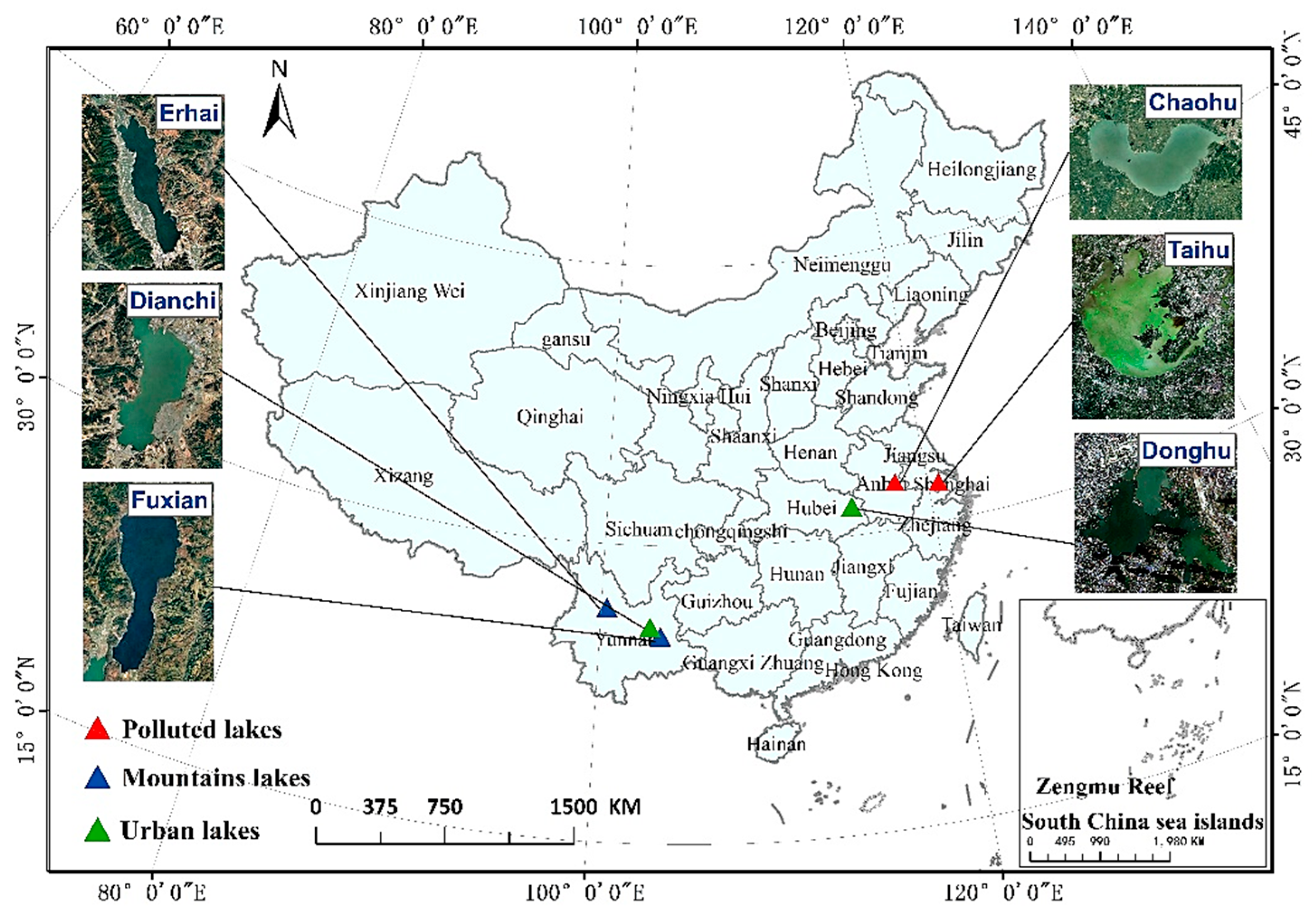
In this study, six inland lakes in China—Dianchi, Donghu, Chaohu, Taihu, Fuxian, and Erhai—covering diverse water body types and complex background environments were selected for assessing the accuracy and adaptability of LWB extraction using Sentinel-1/2 data fusion (Figure 1). Specifically, Lake Chaohu and Taihu are polluted with high chlorophyll concentrations, Lake Fuxian and Erhai are clean and located around the mountains, and Lake Dianchi and Donghu are urban lakes surrounded by cities in complex background environments. The selected lakes fully consider the influence of different geographical environment and water quality for extracting LWB, which can effectively evaluate the effectiveness and adaptability of the proposed method in this paper.
2.1.2. Data
RADAR Sentinel-1 (S1) ground range-detected (GRD) imagery acquired in the interferometric wide swath mode (IW) was fused with Sentinel-2 (S2) multispectral imagery (MSI). The GRD images display backscatter () coefficient values for both vertical (VV) and cross (VH) polarization in dB at a spatial resolution of 20 × 22 m in range and azimuth, respectively. However, the end-user products are provided at a resolution of 10 × 10 m. Sentinel-2 MSI are provided in the form of so-called granules, which cover a ground area of 100 km × 100 km, including 13 spectral bands, with four bands at 10 m, six bands at 20 m, and three bands at 60 m spatial resolution. Its Level-1C standard products provide orthorectified, top-of-atmosphere (TOA) reflectance at sub-pixel multispectral registration. SAR images from Sentinel-1 satellites and optical images from Sentinel-2 are freely downloaded from the Copernicus open access hub (https://scihub.copernicus.eu/, accessed from November to December 2019). Table 2 presents the specifications of the Sentinel-1/2 data.
For training the SVM classifier, 4000 and 3000 water and non-water pixels were selected for each lake, respectively. To evaluate LWB extraction accuracy, 2000 and 1500 test pixels were utilized for water and non-water regions of each lake.
Table 2.
Basic specifications of Sentinel-1/2 data.
| Satellite | Senor Type | Spatial Resolution (m) | Number of Channels | Acquisition Data |
|---|---|---|---|---|
| Sentinel-1 | Optical | 10 | 2 | November–December 2019 |
| Sentinel-2 | RADAR | 10, 20, and 60 | 13 | November–December 2019 |
2.2. Methods
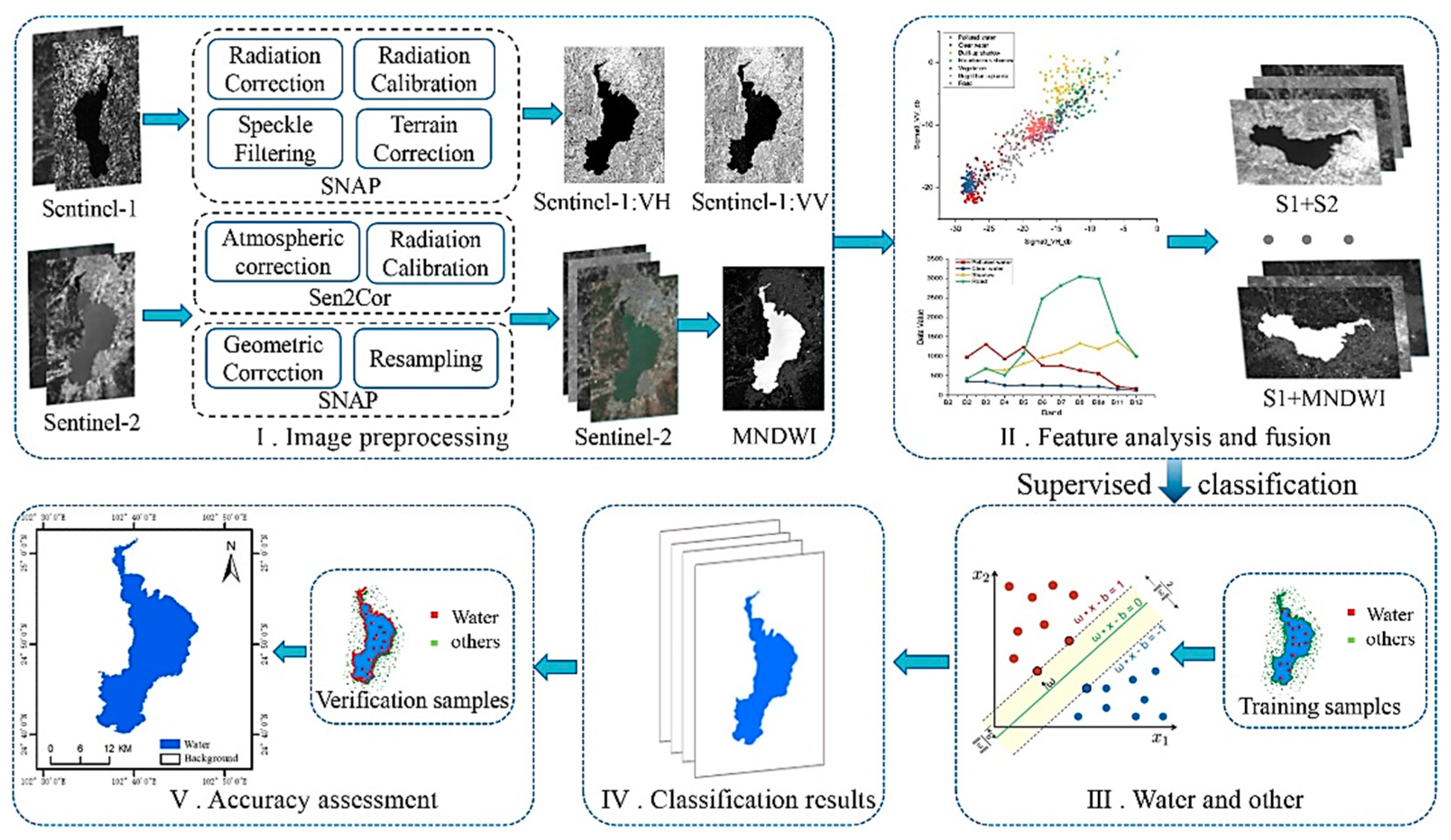
The conceptual diagram of the proposed LWB extraction methodology here is shown in Figure 2. Sentinel-1/2 data were adopted to provide complementary information in sufficient detail. The proposed method consists of three stages: feature analysis and fusion, classification, and accuracy assessment. In the feature analysis and fusion, firstly, the difference of the spectral, polarization, water index features between LWB and non-LWB is analyzed. Then, a combination of spectral polarization and water index are stacked as the inputs of classifier. In the classification, The SVM is applied to extract LWB. Finally, the quantitative accuracy assessment indictors (such as Overall Accuracy (OA), Kappa, Commission Error (CE), and Omission Error (OE)) are adopted to assess accuracy of LWB extraction.
2.2.1. Dataset Preprocessing
The Sentinel Application Platform (SNAP) toolbox developed by the European Space Agency (ESA) was adopted for S1 and S2 preprocessing. The preprocessing of S1 GRD data included border and thermal noise removal, radiometric calibration, and terrain correction implemented using SNAP Sentinel-1 Toolbox processing algorithms [28]. Following these preprocessing steps, geocoded backscatter intensity images were obtained, and the above unitless images were converted to normalized backscatter coefficients (). The two available polarization bands, and , were subsequently extracted at a 10-m spatial resolution [29]. The S2 Level-1C data are ortho-image TOA (top-of-atmosphere) reflectance products, which have been geometrically and radiometrically corrected [30]; therefore, preprocessing consisted of atmospheric correction using the Sen2Cor algorithm to obtain surface reflectance. All S2 spectral bands were then resampled to a 10-m resolution by resampling methods [31].
2.2.2. Water Index
Water indices enhance the spectral differences between LSWBs and non-LSWBs for enhanced water body extraction except for the green, red, and NIR bands because they are very sensitive to water. Several studies have proposed various water indices (NDWI, MNDWI, AWEI) [9,12,14]. The MNDWI can enhance the water features with built-up land in an urban background from LSWBs and was thus selected for optical imagery extraction. The MNDWI combines information from the green and shortwave infrared parts of the spectrum according to Equation (1):
where is the reflectance value of the green band (Band 3 in Sentinel-2 MSI), and is the reflectance value of the SWIR band (Band 11 in Sentinel-2 MSI resampled to a spatial resolution of 10 m).
2.2.3. Features Analysis for LWB Extraction
The LWB extraction from Sentinel-1 SAR data was based on the difference in backscatter coefficient values between water and non-water pixels [25]. Because open water is a smooth surface, C-band radar signals lead to mirror-like reflection and low backscatter values. In contrast, rough non-water surface regions scatter signals in various directions, appearing as high backscatter or bright zones [26]. However, smooth-surface regions (such as sand, roads, and other paved areas) can create specular reflections that cause ambiguity in identifying the LWBs. Wind along the lake surface and phytoplankton in polluted water can also increase roughness, leading to the misclassification of polluted LWBs.
For Sentinel-2 optical data, the spectral reflectance of clear waters, built-up shadow, and mountainous shadow were lower than that of vegetation, bright built-up, and polluted waters; however, the former maintain similar spectral reflectance values across Sentinel-2 bands. If spectral features of Sentinel-2 data are alone used as input, built-up mountainous shadows were easily misclassified to LWB, and clear water and polluted water were misclassified to different types of land-use class.
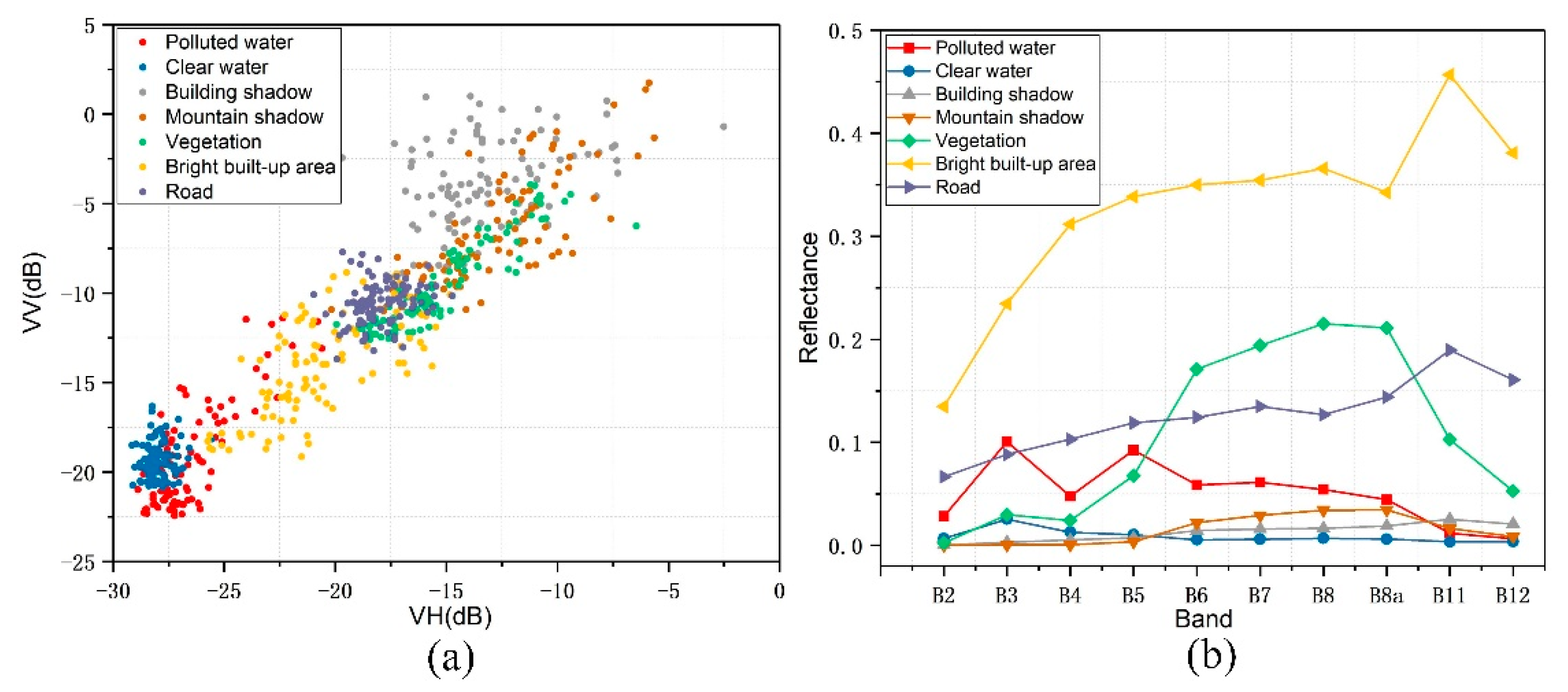
To assess the spectral and polarization feature differences, water and non-water samples were selected to represent the seven land-cover types examined—polluted water, clear water, built-up shadow, mountainous shadow, vegetation, bright built-up, and road—from Sentinel-1/2 imagery within the study regions (Figure 3). Notably, large spectral and polarization differences in feature space were seen between LWBs (clean and polluted water) and all other land-cover types (built-up shadow, mountainous shadow, vegetation, and road).
The backscatter coefficient value of the LWBs was low, with the backscatter coefficient value of VV polarization for polluted water being lower than that of clear water (Figure 3a). Bright buildings had lower backscatter coefficient values for VV polarization, which were similar to those for polluted water. The backscatter coefficient values of roads and vegetation maintained significant differences from LWBs in VV and VH feature space. However, there were significant differences between mountain shadows and building shadows with LWBs in both VV and VH backscatter coefficient values.
The reflectance of LWBs in the visible bands was lower than 10%, with higher reflectance values concentrated in the blue and green bands (Figure 3a). Meanwhile, the reflectance gradually decreases with the increase of the wavelength. The reflectance of clear water in near-infrared band is sharply decreased and is almost equal to zero. Due to the influence of chlorophyll in the polluted water body, the reflectance of the polluted water body in the green band is increased, while the reflectance in the short-wave infrared band is decreased, and the near-infrared band is not completely absorbed. Reflectance of the mountain and building shadows was predictably low, and less than those of clear water for bands 2, 3, and 4. In the bands 6, 7, 8, 8a, 11, and 12, the reflectance of mountain shadows and building shadows was slightly higher than clear water. A small peak in vegetation reflection can be seen in the visible bands, while NIR reflectance rapidly increased, and SWIR reflectance decreased. There spectral differences between roads, bright buildings, and clear water were significant.
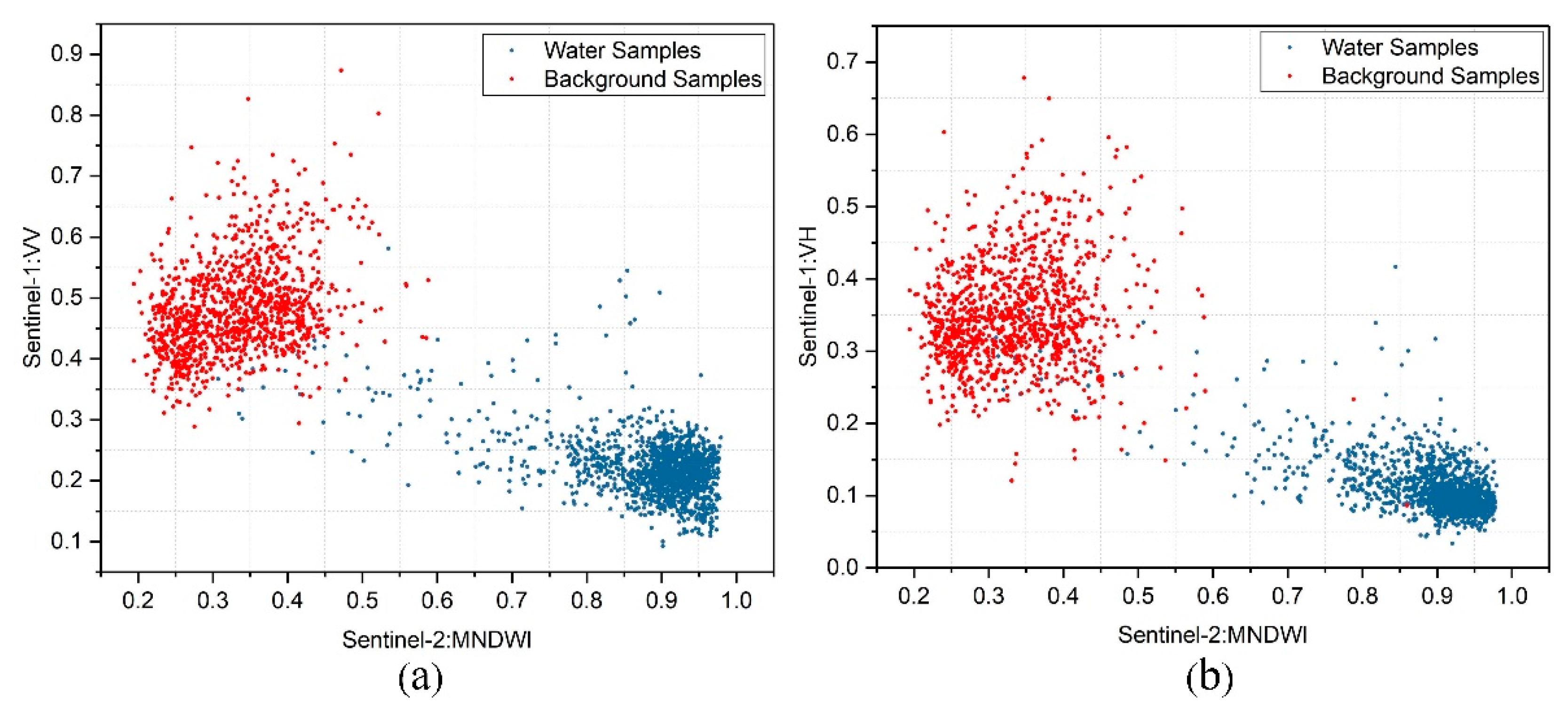
Although water indices have been widely applied in the literature to extract surface water bodies, methods used to determine an optimal threshold between water and non-water greatly influence the extraction accuracy; therefore, different optimal threshold values were chosen to extract water bodies from different geographical environments. Numerous studies have indicated that water only becomes clearly separable when the feature space (spectral feature, backscatter coefficient of VV and VH feature, water indices feature) is extended to two or three dimensions [27]. Accordingly, samples of water and non-water background were collected for Sentinel-1 SAR and MNDWI data within the experimental region, and scatter plots of VV/VH and MNDWI show a clear discrimination in two-dimensional feature space (Figure 4). Therefore, comprehensive use of the spectral, polarization, and MNDWI features by fusing the Sentinel-1/2 data to extract LWB can overcome the shortcomings of single optical or radar data and enhance the differences between LWB and background objects.
2.2.4. Feature Fusion for LWB Extraction
As mentioned in Section 2.2.3, increasing the dimensionality of the feature space can improve the separability of water body from the non-water background. Accordingly, the feature space here was extended to multiple dimensions by fusing the spectral features and MNDWI of Sentinel-2 with VV/VH backscatter features of Sentinel-1. As the dimensions are inconsistent between the three feature types, the data were first normalized into (0, 1) in such a way that they could then be fused into the classifier. The normalized method was adopted in the present study, which can be formulated according to Equation (2) [32]:
where denotes the original feature value of the pixel ; and represent the maximum and minimum values of that feature, respectively; and is the feature value of pixel after normalization.
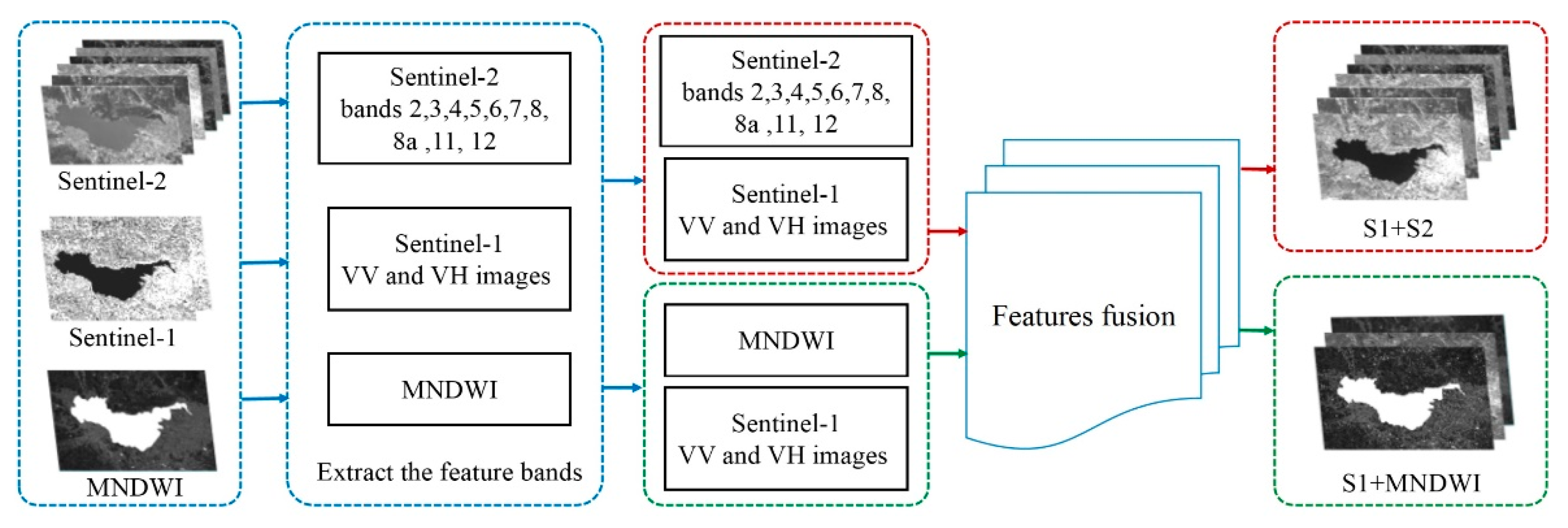
Image fusion methods can be classified into three different levels: pixel, feature, and decision [33]. The most relevant method of data fusion is to combine features in order to create value added features. In this study, feature stacking was employed for feature fusion. In the first fusion scheme, Sentinel-2 bands 2, 3, 4, 5, 6, 7, 8, 8a, 11, 12, and Sentinel-1 VV and VH were fused to a 12 dimensional features by feature stacking. In the second fusion scheme, MNWDI data and Sentinel-1 VV and VH were fused to three-dimensional features by feature stacking (the conceptual fusion frameworks are illustrated in Figure 5).
2.2.5. Classification Method
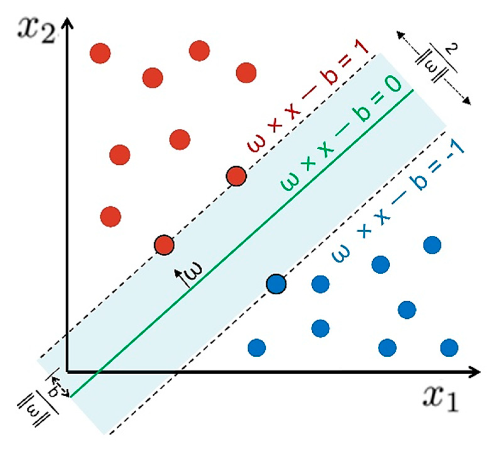
Support vector machine is a machine-learning algorithm based on statistical learning theory [34], and has been widely used for remote sensing image classification because of the small number of training samples required and high-dimensional space [35]. Accordingly, SVM was adopted to extract LWBs across the study area based on the inputs of the two fused datasets. Originally introduced to solve linear, binary classification problems, the general idea of SVMs is to classify training samples by tracing maximum margin hyperplanes in the feature space; however, multidimensional features created by fusing Sentinel-1 and 2 data are typically nonlinear. To increase the suitability of the SVM to multidimensional features, they can be generalized to a non-linear decision function by employing the kernel trick [36], where a kernel-based SVM is used to project the pixel vectors into a higher dimensional space and estimate the corresponding maximum margin hyperplanes in order to improve the linear separability of features. Among the different types of kernels, the Gaussian radial basis function (RBF) has been widely applied for remote sensing classification.
A binary SVM (water and non-water) was employed here. The form of SVM classifiers is defined by Equation (3), which is in turn learned from the data , where is an n-dimensional feature vector, and is a sample label [37]. The conceptual principle of SVM is illustrated in Figure 6:
where denotes a hyperplane that separates the sample label on each side, and and are the parameters of the hyperplane.
Subsequently, the hyperplane calculation can be expressed as a constrained optimization formula according to Equation (4) [32]:
where C is a regularization parameter, and denotes slack-variables subject to the constraints of Equation (5):
2.2.6. Accuracy Assessment
To quantitatively evaluate the performance of LWB extraction under the proposed methods, the four adopted evaluation metrics were calculated according to Equations (6)–(9) [3,38]:
where TP denotes true positives, i.e., the number of LWB pixels correctly detected; FP denotes false positives, i.e., the number of LWB pixels incorrectly detected; TN and FN denote true and false negatives, respectively; and .
2.2.7. Experiment Design
To evaluate performance, five sets of input features were used in the SVM classifier: Sentinel-2 spectral bands only, MNDWI only, Sentinel-1 VV and VH only, fusion of spectral bands and dual polarization, and the fusion of MNDWI and dual polarization (Table 3).
Generally, the robustness of the LSWB extraction method is predominantly affected by the spectral diversity of water bodies and the heterogeneity of adjacent surfaces across different geographical regions. Six test sites characterizing three lake types—clean, polluted, mountain, and urban—were selected to perform a comprehensive analysis of LWB extraction efficiency. In this study, the libSVM software package in MATLAB (2016a) was used to extract LWB, and the RBF was adopted as the SVM kernel function.
3. Results
3.1. LWB Extraction Performance
The classification results are shown in Figure 7. In Method I (MNDWI only), the reflectivity of buildings in the MIR band was stronger than that of the NIR band. Accordingly, employing the MIR band in the exponential model construction allowed the MNDWI to effectively suppress noise interference from buildings and shadows. In the extracted results, there was a small amount of shadow information interference from buildings and mountains. For Taihu and Chaohu Lake, the extraction of the lake water surface was incomplete due to the floating cyanobacteria along the surface.
When we applied the proposed Method II (S1 only), we did not obtain good extraction results. The low backscatter coefficients of bright buildings were similar to those of water bodies, leading to misclassification in the extraction results. In urban lakes, the background of the ground features was complicated and lead to an abundance of speckle noise and misclassified areas. Method III (S2 only), the reflectivity of shadows was similar to that of water bodies from the visible light band (b2) to the NIR band (b8). This resulted in incorrectly classifying shadows as water bodies. In addition, cyanobacteria floating on the surface of water bodies were classified as vegetation, resulting in the incomplete extraction of Taihu and Chaohu Lake.
Methods IV and V (Sentinel-1/2 data fusion) not only overcame the influence of shadows and low-reflectivity ground objects but effectively suppressed the interference of smooth ground objects as well; thus, optical and radar data functioned complimentarily, improving the overall LSWBs extraction effect. As shown in Figure 7, Table 4 and Table 5, the overall misclassification area of the six lakes was significantly reduced, the boundaries were clear, and the water body was complete in the results from the fusion techniques.
Figure 7.
Comparison of LWB extraction results for Methods I–V at each of the six test sites.

3.2. Accuracy Assessment
Figure 8 presents the visual comparisons of the results by different methods, and the first column shows the original images. Specifically, as shown in the first rows of Figure 8, the use of radar data in Method II can completely extract the tortuous boundaries of the islands in the lake, but the extraction of the land in the island is incomplete. In Methods I and III, the optical data cannot be used to describe the true water-land boundary due to the influence of vegetation on the waterside, but the island land is extracted completely. In Methods IV and V, the island land and the curved boundary are completely extracted. In the second and third rows of Figure 8, Methods I and III cannot extract water bodies covered with cyanobacteria and phytoplankton, and Methods IV and V can completely extract water bodies. In the fourth row of Figure 8, for the extraction of dark water bodies on optical images, Methods I and III do not perform well. As seen in the last row of Figure 8, Method II cannot extract the roads connecting islands in the lake, and the fusion data can completely extract the roads in the water. Thus, benefiting from the advantages of the complementarity of optical data and radar data, the fusion methods show good performance when extracting LSWBs in complex environments.
In order to better analyze the LSWBs extraction results of the six lakes, a series of quantitative accuracy indices was used (Table 4). Overall, Methods IV and V obtained the highest classification accuracy using Sentinel-1/2 data fusion. For Method IV, the overall accuracy for each of the six lake extractions was ≥94.72%, and the Kappa coefficient was ≥0.88. For Method V, the overall accuracy was ≥95.28%, and the Kappa coefficients were ≥0.89. The next most accurate were Methods I and II. In Method I, the overall accuracies of all lakes was 89.63–93.01; and Kappa coefficients were 0.80–0.87. In Method II, the overall accuracies of all lakes were 88.21–93.08; Kappa coefficients were 0.77–0.87. Method III maintained the lowest classification accuracies. For Method III, the overall accuracy of all lakes was between 88.15 and 93.17 and Kappa coefficients between 0.71–0.86.
Table 4.
Accuracy calculations across the six lakes.
| Scheme | Donghu | Dianchi | Fuxian | Erhai | Taihu | Chaohu | ||||||
|---|---|---|---|---|---|---|---|---|---|---|---|---|
| OA% | Kappa | OA% | Kappa | OA% | Kappa | OA% | Kappa | OA% | Kappa | OA% | Kappa | |
| I | 91.04 | 0.85 | 93.01 | 0.87 | 92.79 | 0.86 | 89.63 | 0.80 | 92.11 | 0.84 | 91.35 | 0.85 |
| II | 88.21 | 0.77 | 91.24 | 0.83 | 93.08 | 0.87 | 92.04 | 0.85 | 90.01 | 0.80 | 89.76 | 0.80 |
| III | 90.13 | 0.84 | 93.17 | 0.86 | 92.13 | 0.85 | 88.15 | 0.71 | 91.87 | 0.83 | 91.11 | 0.84 |
| IV | 95.29 | 0.91 | 96.53 | 0.92 | 96.32 | 0.95 | 97.06 | 0.94 | 95.42 | 0.91 | 94.72 | 0.88 |
| V | 95.87 | 0.91 | 96.77 | 0.93 | 97.07 | 0.95 | 97.93 | 0.96 | 95.51 | 0.91 | 95.28 | 0.89 |
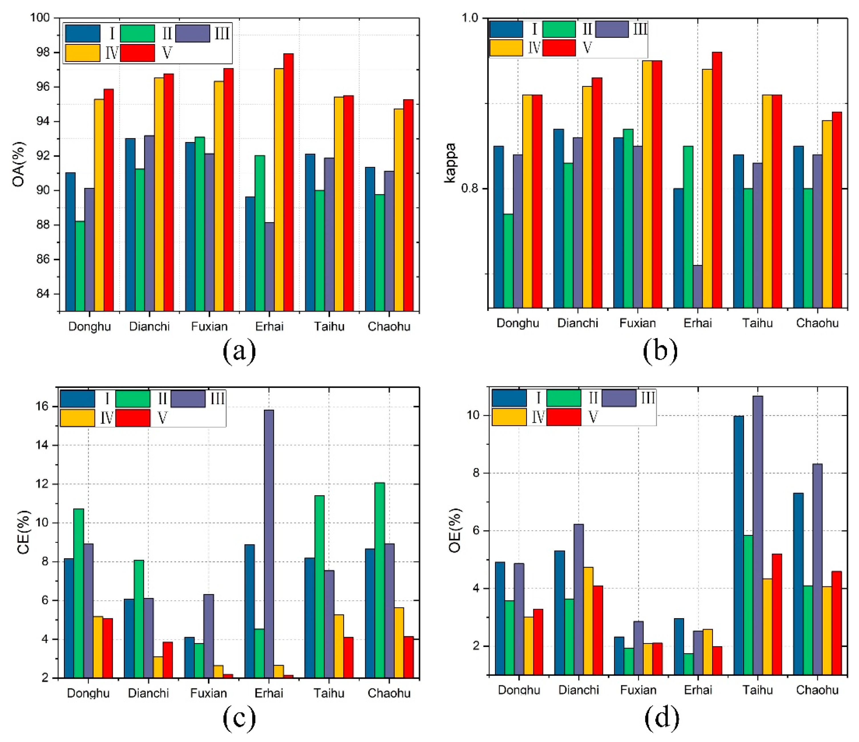
Additionally, Methods IV and V maintained the lowest levels of classification error (Table 5, Figure 9), indicating that both wrong and missed points were improved under the fusion techniques. Methods I and III held the highest commission error in mountainous lakes, with lower errors of misclassification and higher errors of omission in other lakes. Method II obtained higher error of misclassification and lower error of omission.
Table 5.
Error calculations across the six lakes.
| Scheme | Donghu | Dianchi | Fuxian | Erhai | Taihu | Chaohu | ||||||
|---|---|---|---|---|---|---|---|---|---|---|---|---|
| CE% | OE% | CE% | OE% | CE% | OE% | CE% | OE% | CE% | OE% | CE% | OE% | |
| I | 8.15 | 4.91 | 6.07 | 5.31 | 4.09 | 2.32 | 8.87 | 2.96 | 8.18 | 9.98 | 8.66 | 7.31 |
| II | 10.73 | 3.57 | 8.08 | 3.64 | 3.78 | 1.94 | 4.53 | 1.74 | 11.41 | 5.84 | 12.07 | 4.10 |
| III | 8.92 | 4.86 | 6.10 | 6.23 | 6.31 | 2.86 | 15.81 | 2.52 | 7.54 | 10.67 | 8.93 | 8.31 |
| IV | 5.17 | 3.02 | 3.09 | 4.73 | 2.64 | 2.09 | 2.65 | 2.59 | 5.26 | 4.34 | 5.63 | 4.07 |
| V | 5.08 | 3.29 | 3.85 | 4.09 | 2.19 | 2.11 | 2.15 | 1.98 | 4.09 | 5.19 | 4.14 | 4.59 |
4. Discussion
From the above results, it can be seen that the method of fusing Sentinel 1/2 data to extract LWB has the better performance. Compared with the traditional water index method, it has higher extraction accuracy and lower error. MNDWI is simple to calculate and can quickly generate water maps. However, the determination of the water index threshold will change with time and space, especially in complex environments, such as cities and mountainous areas. A large amount of background information has a strong interference in the determination of the threshold. Therefore, in order to better determine whether the fusion method proposed in this study is suitable for LWB extraction in a complex environment, lake environmental noise, lake water-body type, and computational complexity are discussed.
4.1. Lake Environmental Noise
Extracting water bodies in a complex geographic environment is susceptible to interference from a number of sources (e.g., shadows, buildings, forest vegetation) leading to poor extraction accuracy. However, in LSWBs extraction, such sources of environmental noise present can help categorize lakes into urban lakes and mountain LSWBs.
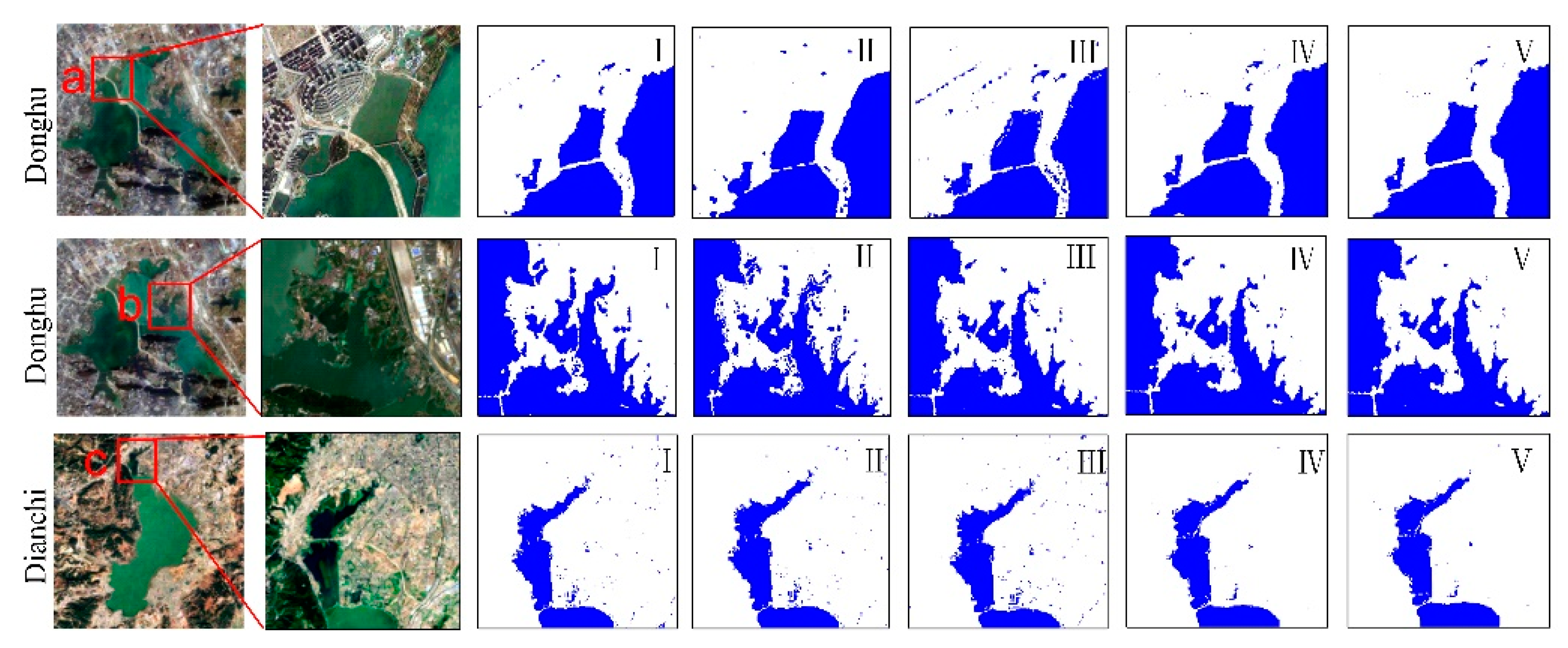
Urban lakes maintain a complex background environment. In the Sentinel-2 optical imagery, there is interference from building shadows and other low-reflectance features. Methods incorporating radar polarization information overcome the influence of the spectral heterogeneity of ground objects; however, they remain susceptible to smooth ground objects (e.g., bright buildings), creating false positives. Figure 10a,b is enlarged partial views of the Donghu Lake composite image according to the extraction results of the five methods. Area a, in the northwest part of the lake, was affected by buildings and shadows, creating low LSWBs extraction accuracy values for Methods I–III. Conversely, Methods IV and V reduced the interference of background objects and more completely extracted the LSWBs. Area b in the northeastern part of Donghu Lake suffered from the interference of buildings, mountain shadows, highly reflective surfaces, and roads. Accordingly, Methods I–III did not perform well, whereas Methods IV and V performed better. Area c in the northern part of Dianchi Lake is close to the urban area and contained complex background features. Affected by building shadows, vegetation, roads, etc., the extraction results of Methods I–III are not good, and there are a great deal of speckle noises around the lake. However, Methods IV and V could effectively distinguish the water and non-water pixels. These methods reduced the impact of ground object disturbance, more completely identifying LSWBs in the complex areas and producing a smooth and continuous water boundary with improved accuracy and reduced error rates.
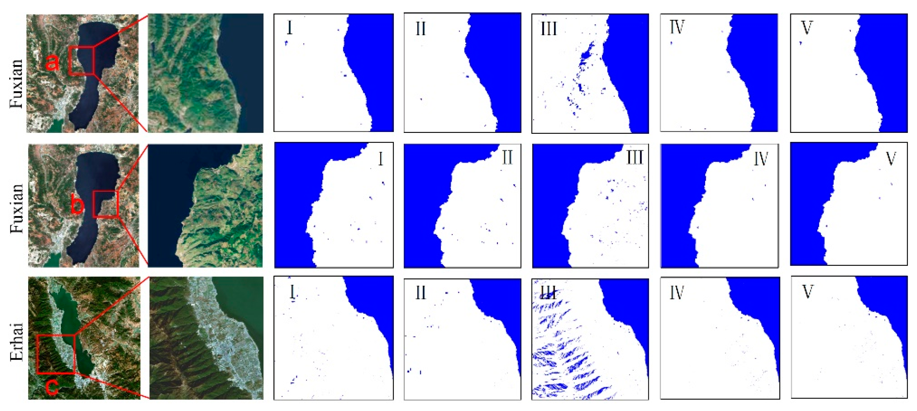
The extraction process for montane lakes in plateau areas was primarily affected by mountain shadows and vegetation. In view of the limitations of remote sensing spectral information in complex geographic environments, mountain shadows were often incorrectly identified as water bodies. LSWBs concealed under vegetation along the land boundary area were prone to mix. As showed in Figure 11, areas a and b are located in the montane areas on the west and east sides of Fuxian Lake, respectively. Figure 11c shows an area along the southwest bank of the plateau of Lake Erhai, close to the mountains. Affected by the shadows of the mountains, there were weak patches that were incorrectly identified as water in Method I, and a large number of background objects were incorrectly identified as water in Method III. Due to the influence of the so-called radar shadow (during the imaging process, the top of the mountain is closer to the sensor than the bottom of the mountain, which will cause the object to appear to “collapse” towards the sensor) of the radar sensor, some misclassifications also occurred in Method II. Fusion Methods IV and V, however, effectively improved extraction results.
4.2. Lake Water Body Types
The LWB extraction was also affected by water quality. To verify the adaptability of the proposed methods, lakes were divided into clean and polluted states. Overall, the water quality of clean lakes Erhai and Fuxian maintained low turbidity, chlorophyll concentrations, and clear lake boundaries. It can be seen from the extraction results that, in Method III, the surrounding mountain shadows are wrongly extracted as water bodies. In methods I and II, there were also a small amount of wrong extraction around the lake. In general, although there were some commission errors, for the extraction of LSWBs, all five methods can be completely extracted.
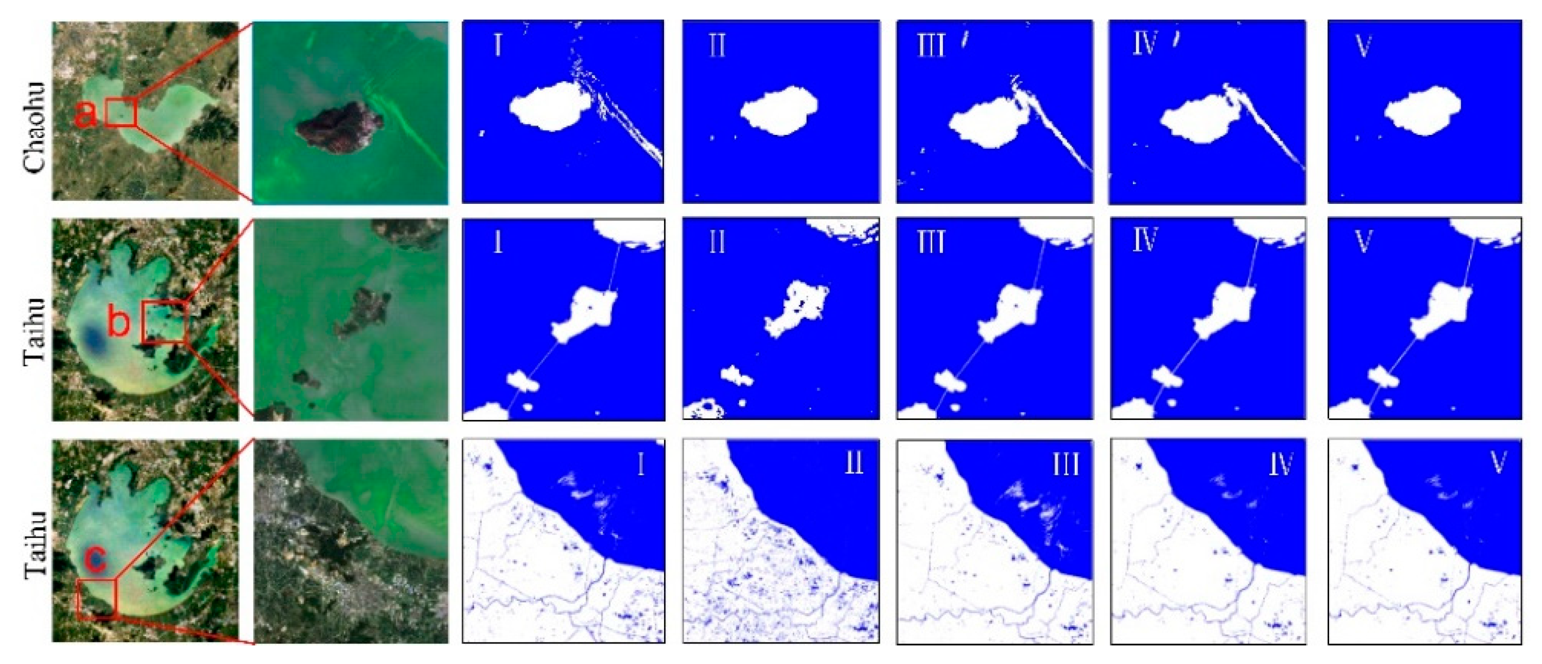
Alternatively, Chaohu and Taihu lakes were considered polluted. Figure 12a displays the island-containing area of Chaohu Lake, and the surrounding chlorophyll concentrations were relatively high. Methods I and III produced poor, incomplete extractions due to the influence of cyanobacteria. In Method II, the water body containing algae was more completely extracted. Method V maintained the highest extraction accuracy, overcoming the interference of cyanobacteria and more completely separating the islands. Method IV reduced the influence of algae to a certain extent albeit inferior to Method V. Area b contains small islands in Taihu Lake and roads connecting the islands. It can be seen from Figure 12b that Methods I and III extracted roads in lakes, but Method II cannot extract roads, and the extracted islands are incomplete and broken. The fusion Methods IV and V clearly extract the complete islands and roads. Area c presents the chlorophyll concentrated boundaries on the south side of Taihu Lake. Methods I and III suffered from interference by algae, leading to incomplete LWB extractions. In Method II, S1 radar data largely avoided interference of algae but were affected by the surrounding urban buildings, creating numerous misclassifications with discontinuous and incompletely extracted LSWBs in the boundary areas. Under Methods IV and V, the LSWBs were more completely extracted, and the effects of LSWBs containing cyanobacterial blooms were effectively eliminated. At the same time, it also reduced the interference of the surrounding environment noise, and the error extraction was reduced.
4.3. Computational Complexity
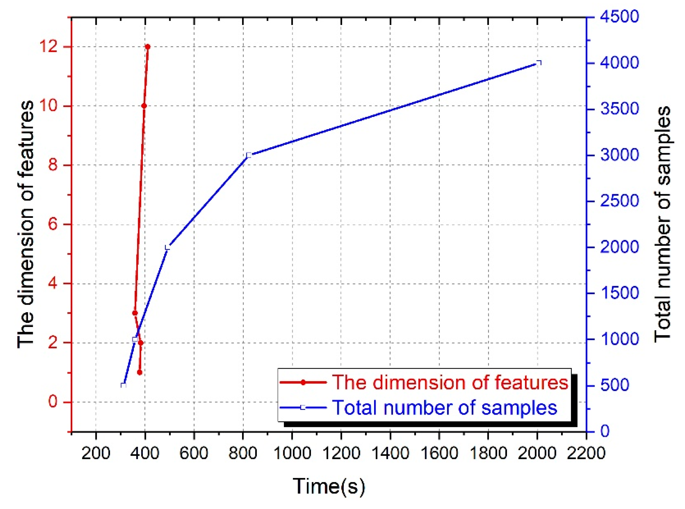
In this paper, the LWB extraction mainly includes three steps: feature analysis and extraction, feature fusion, and classification. In the feature analysis and extraction stage, the operation is simple, and the computational complexity is low. Feature fusion mainly uses the layer stacking to generate multidimensional data from Sentinel-1/2 data, and this process is also relatively low in computational complexity. Therefore, the computational complexity of the entire process mainly depends on the efficiency of SVM. The complexity of SVM is considered from the following two aspects: the dimensions of features and total number of samples. We set up two sets of experiments to verify: (1) The number of training samples remains unchanged at 1000; the feature dimensions of the input classifier are: 1, 2, 3, 10, and 12 (the same as the feature dimensions of the five methods proposed in this study); and the running time under different feature dimensions is recorded. (2) The feature dimension is 1 and remains unchanged; the numbers of input training samples are: 500, 1000, 2000, 3000, 4000; and the running time under different number of samples is recorded.
As shown in Figure 13, it can be found that the computational complexity of SVM has nothing to do with the dimensionality of features; rather, it is related to the total number of training samples and depends on the number of support vectors [39]. Therefore, the computational complexity will not increase as the dimension of features changes. Compared with water index method, the method by fusing Sentinel-1/2 data is still an efficient approach.
5. Conclusions
In this study, we developed a method for automated extraction lake surface water bodies in complex geographical environments by fusing Sentinel-1/2 data, which integrated the advantages of optical and radar remotely sensed products to accurately and automatically mapping LSWBs. The extraction results using data fusion methods and other three methods (Sentinel-1 only, Sentinel-2 only, and MNDWI) were tested for six different lakes of China having different types, and results showed that: (1) fusion of Sentinel-1/2 data to extract LWB achieved good results in various types of lakes and effectively suppressed the effects of shadows, water quality, and smooth-surface features. (2) The fusion method performed well with an overall accuracy of 94.48% to 97.93%. Compared with other methods, the accuracy was significantly improved while maintaining water-boundary continuity and lake-surface completion. (3) The classification error of fusion method was less than 6% in all lakes and could reduce the error significantly than other three methods.
Experiments on six different types of lakes under complex environments indicated that the proposed methods were applicable to various types of LWB extraction, showing an extremely robustness over the time. In future research, we will explore the possibility of the proposed method for large-scale surface-water mapping and conduct research on the classification of surface water bodies that takes into account local background information.
Author Contributions
Conceptualization, L.H.; data curation, M.L. and J.G.; formal analysis, M.L. and J.G.; methodology, M.L.; writing—original draft, M.L.; writing—review and editing, L.H. and A.Z. All authors have read and agreed to the published version of the manuscript.
Funding
This work was funded by the National Natural Science Foundation of China (Grant Nos. 42171392; 41861048; 41971369); and Yunnan Province Young Academic and Technical Leaders Reserve Talent Project (Grant No. 202105AC160059); and Yunnan Province Basic Research Special Key Project (No. 202001AS070032).
Institutional Review Board Statement
Not applicable for studies not involving humans or animals.
Informed Consent Statement
Not applicable.
Data Availability Statement
The data presented in this study are openly available in Copernicus open access hub at https://scihub.copernicus.eu (accessed on 9 November 2021).
Conflicts of Interest
The authors declare no conflict of interest.
Appendix A
Table A1.
List of acronyms.
| Acronyms | Full Name |
|---|---|
| LWB | Lake water body |
| LSWB | Land surface water body |
| SAR | Synthetic aperture radar |
| S1 | Sentinel-1 |
| S2 | Sentinel-2 |
| SVM | Support vector machine |
References
- Huang, L.; Xu, X.; Zhai, J.; Sun, C. Local background climate determining the dynamics of plateau lakes in China. Reg. Environ. Chang. 2016, 16, 2457–2470. [Google Scholar] [CrossRef]
- Wu, P.; Shen, H.; Cai, N.; Zeng, C.; Wu, Y.; Wang, B. Spatiotemporal analysis of water area annual variations using a Landsat time series: A case study of nine plateau lakes in Yunnan province, China. Int. J. Remote Sens. 2016, 37, 5826–5842. [Google Scholar] [CrossRef]
- Wang, Z.; Gao, X.; Zhang, Y.; Zhao, G. MSLWENet: A Novel Deep Learning Network for Lake Water Body Extraction of Google Remote Sensing Images. Remote Sens. 2020, 12, 4140. [Google Scholar] [CrossRef]
- Xu, Y.; Liu, W.; Song, J.; Yao, L.; Gu, S. Dynamic Monitoring of the Lake Area in the Middle and Lower Reaches of the Yangtze River Using MODIS Images Between 2000 and 2016. IEEE J. Sel. Top. Appl. Earth Obs. Remote Sens. 2018, 11, 4690–4700. [Google Scholar] [CrossRef]
- Jiang, H.; Feng, M.; Zhu, Y.; Lu, N.; Huang, J.; Xiao, T. An Automated Method for Extracting Rivers and Lakes from Landsat Imagery. Remote Sens. 2014, 6, 5067–5089. [Google Scholar] [CrossRef] [Green Version]
- Du, Y.; Zhang, Y.; Ling, F.; Wang, Q.; Li, W.; Li, X. Water Bodies’ Mapping from Sentinel-2 Imagery with Modified Normalized Difference Water Index at 10-m Spatial Resolution Produced by Sharpening the SWIR Band. Remote Sens. 2016, 8, 354. [Google Scholar] [CrossRef] [Green Version]
- Zhang, G.; Zheng, G.; Gao, Y.; Xiang, Y.; Lei, Y.; Li, J. Automated Water Classification in the Tibetan Plateau Using Chinese GF-1 WFV Data. Photogramm. Eng. Remote Sens. 2017, 83, 509–519. [Google Scholar] [CrossRef]
- Work, E.; Gilmer, D.S. Utilization of satellite data for inventorying prairie ponds and lakes. Photogramm. Eng. Remote Sens. 1976, 42, 685–694. [Google Scholar]
- McFeeters, S.K. The use of the Normalized Difference Water Index (NDWI) in the delineation of open water features. Int. J. Remote Sens. 1996, 17, 1425–1432. [Google Scholar] [CrossRef]
- Yang, X.; Qin, Q.; Grussenmeyer, P.; Koehl, M. Urban surface water body detection with suppressed built-up noise based on water indices from Sentinel-2 MSI imagery. Remote Sens. Environ. 2018, 219, 259–270. [Google Scholar] [CrossRef]
- Li, W.; Du, Z.; Ling, F.; Zhou, D.; Wang, H.; Gui, Y. A Comparison of Land Surface Water Mapping Using the Normalized Difference Water Index from TM, ETM+ and ALI. Remote Sens. 2013, 5, 5530–5549. [Google Scholar] [CrossRef] [Green Version]
- Xu, H. Modification of normalised difference water index (NDWI) to enhance open water features in remotely sensed imagery. Int. J. Remote Sens. 2006, 27, 3025–3033. [Google Scholar] [CrossRef]
- Li, L.; Su, H.; Du, Q.; Wu, T. A novel surface water index using local background information for long term and large-scale Landsat images. ISPRS J. Photogramm. Remote Sens. 2021, 172, 59–78. [Google Scholar] [CrossRef]
- Feyisa, G.L.; Meilby, H.; Fensholt, R.; Proud, S.R. Automated Water Extraction Index: A new technique for surface water mapping using Landsat imagery. Remote Sens. Environ. 2014, 140, 23–35. [Google Scholar] [CrossRef]
- Wang, X.; Xie, S.; Zhang, X.; Chen, C.; Guo, H.; Du, J. A robust Multi-Band Water Index (MBWI) for automated extraction of surface water from Landsat 8 OLI imagery. Int. J. Appl. Earth Obs. Geoinf. 2018, 68, 73–91. [Google Scholar] [CrossRef]
- Ciuonzo, D.; Carotenuto, V.; De Maio, A. On multiple covariance equality testing with application to SAR change detection. IEEE Trans. Signal Process. 2017, 65, 5078–5091. [Google Scholar] [CrossRef]
- Saha, S.; Bovolo, F.; Bruzzone, L. Building change detection in VHR SAR images via unsupervised deep transcoding. IEEE Trans. Geosci. Remote Sens. 2020, 59, 1917–1929. [Google Scholar] [CrossRef]
- Wang, Z.L.; Liao, M.S.; Zhang, L. Detecting and characterizing deformations of the left bank slope near the Jinping hydropower station with time series Sentinel-1 data. Remote Sens. Land Resour. 2019, 31, 204–209. [Google Scholar]
- Tian, H.; Li, W.; Wu, M.; Huang, N.; Li, G.; Li, X. Dynamic Monitoring of the Largest Freshwater Lake in China Using a New Water Index Derived from High Spatiotemporal Resolution Sentinel-1A Data. Remote Sens. 2017, 9, 521. [Google Scholar] [CrossRef] [Green Version]
- Zhang, Y.; Zhang, G.; Zhu, T. Seasonal cycles of lakes on the Tibetan Plateau detected by Sentinel-1 SAR data. Sci. Total Environ. 2019, 703, 135563. [Google Scholar] [CrossRef]
- Valdiviezo-Navarro, J.C.; Salazar-Garibay, A.; Téllez-Quiñones, A.; Orozco-del-Castillo, M.; López-Caloca, A.A. Inland water body extraction in complex reliefs from Sentinel-1 satellite data. J. Appl. Remote Sens. 2019, 13, 016524. [Google Scholar] [CrossRef]
- Saghafi, M.; Ahmadi, A.; Bigdeli, B. Sentinel-1 and Sentinel-2 data fusion system for surface water extraction. J. Appl. Remote Sens. 2021, 15, 014521. [Google Scholar] [CrossRef]
- Guo, H.D. Analysis of Radar Remote Sensing Imagery in China; Science Press: Beijing, China, 1999. [Google Scholar]
- Guo, H.D. Spaceborne Multifrequency, Polarametric and Interferometric Radar for Detection of the Targets on Earth Surface and Subsurface. J. Remote Sens. 1997, 1, 32–39. [Google Scholar]
- Bioresita, F.; Puissant, A.; Stumpf, A.; Malet, J.-P. Fusion of Sentinel-1 and Sentinel-2 image time series for permanent and temporary surface water mapping. Int. J. Remote Sens. 2019, 40, 9026–9049. [Google Scholar] [CrossRef]
- Slinski, K.M.; Hogue, T.S.; McCray, J.E. Active-Passive Surface Water Classification: A New Method for High-Resolution Monitoring of Surface Water Dynamics. Geophys. Res. Lett. 2019, 46, 4694–4704. [Google Scholar] [CrossRef]
- Schmitt, M. Potential of Large-Scale Inland Water Body Mapping from Sentinel-1/2 Data on the Example of Bavaria’s Lakes and Rivers. PFG J. Photogramm. Remote Sens. Geoinf. Sci. 2020, 88, 271–289. [Google Scholar] [CrossRef]
- Mahdianpari, M.; Salehi, B.; Mohammadimanesh, F.; Homayouni, S.; Gill, E. The first wetland inventory map of newfoundland at a spatial resolution of 10 m using sentinel-1 and sentinel-2 data on the google earth engine cloud computing platform. Remote Sens. 2019, 11, 43. [Google Scholar] [CrossRef] [Green Version]
- Poortinga, A.; Tenneson, K.; Shapiro, A.; Nquyen, Q.; San Aung, K.; Chishtie, F. Mapping plantations in Myanmar by fusing landsat-8, sentinel-2 and sentinel-1 data along with systematic error quantification. Remote Sens. 2019, 11, 831. [Google Scholar] [CrossRef] [Green Version]
- Li, C.; Shao, Z.; Zhang, L.; Huang, X.; Zhang, M. A comparative analysis of index-based methods for impervious surface extraction using multi-seasonal Sentinel-2 satellite data. IEEE J. Sel. Top. Appl. Earth Obs. Remote Sens. 2021, 14, 3682–3694. [Google Scholar] [CrossRef]
- Tavares, P.A.; Beltrão, N.E.S.; Guimarães, U.S.; Teodoro, A.C. Integration of Sentinel-1 and Sentinel-2 for Classification and LULC Mapping in the Urban Area of Belém, Eastern Brazilian Amazon. Sensors 2019, 19, 1140. [Google Scholar] [CrossRef] [Green Version]
- Liangpei, Z.; Xin, H.; Bo, H.; Pingxiang, L. A pixel shape index coupled with spectral information for classification of high spatial resolution remotely sensed imagery. IEEE Trans. Geosci. Remote Sens. 2006, 44, 2950–2961. [Google Scholar] [CrossRef]
- Liu, Z.; Blasch, E.; Bhatnagar, G.; John, V.; Wu, W.; Blum, R.S. Fusing synergistic information from multi-sensor images: An overview from implementation to performance assessment. Inf. Fusion 2018, 42, 127–145. [Google Scholar] [CrossRef]
- Cortes, C.; Vapnik, V. Support-vector networks. Mach. Learn. 1995, 20, 273–297. [Google Scholar] [CrossRef]
- Mountrakis, G.; Im, J.; Ogole, C. Support vector machines in remote sensing: A review. ISPRS J. Photogramm. Remote Sens. 2011, 66, 247–259. [Google Scholar] [CrossRef]
- Pullanagari, R.; Kereszturi, G.; Yule, I.J.; Ghamisi, P. Assessing the performance of multiple spectral–spatial features of a hyperspectral image for classification of urban land cover classes using support vector machines and artificial neural network. J. Appl. Remote Sens. 2017, 11, 026009. [Google Scholar] [CrossRef] [Green Version]
- Melgani, F.; Bruzzone, L. Classification of hyperspectral remote sensing images with support vector machines. IEEE Trans. Geosci. Remote Sens. 2004, 42, 1778–1790. [Google Scholar] [CrossRef] [Green Version]
- Zhang, Z.; Zhang, X.; Jiang, X.; Xin, Q.; Ao, Z.; Zuo, Q. Automated Surface Water Extraction Combining Sentinel-2 Imagery and OpenStreetMap Using Presence and Background Learning (PBL) Algorithm. IEEE J. Sel. Top. Appl. Earth Obs. Remote Sens. 2019, 12, 3784–3798. [Google Scholar] [CrossRef]
- Chen, L.; Chen, J.; Gao, X.; Wang, L. Research on classification algorithm based on Support vector machine and anti-K nearest Neighbor. Comput. Eng. Appl. 2010, 46, 135–138. [Google Scholar]
Figure 1.
Geographic locations and optical imagery of the six lakes examined. The images shown are a false-color composite (Bands 8, 4, and 3) of Sentinel-2 MSI data.
Figure 1.
Geographic locations and optical imagery of the six lakes examined. The images shown are a false-color composite (Bands 8, 4, and 3) of Sentinel-2 MSI data.

Figure 2.
Conceptual workflow of the proposed data fusion method.

Figure 3.
Feature space plots for seven land cover types sampled. (a) Polarization, S1 and (b) spectral, S2 differences.
Figure 3.
Feature space plots for seven land cover types sampled. (a) Polarization, S1 and (b) spectral, S2 differences.

Figure 4.
Water and non-water background samples plotted in feature space formed by Sentinel-1: (a) VV and (b) VH backscatter vs. Sentinel-2 MNDWI.
Figure 4.
Water and non-water background samples plotted in feature space formed by Sentinel-1: (a) VV and (b) VH backscatter vs. Sentinel-2 MNDWI.

Figure 5.
The conceptual fusion framework of Sentinel-1/2 spectral and polarization data.

Figure 6.
Conceptual principle of the SVM.

Figure 8.
Visual comparisons of the results by different Methods I–V.

Figure 9.
Accuracy analysis across the six lakes. (a) Overall accuracy. (b) Kappa coefficients. (c) Commission error. (d) Omission error.
Figure 9.
Accuracy analysis across the six lakes. (a) Overall accuracy. (b) Kappa coefficients. (c) Commission error. (d) Omission error.

Figure 10.
Comparison of LWB extraction in urban lakes across Methods I–V. The subs (a–c) of Figure 10 are used to show the differences among the extraction results.
Figure 10.
Comparison of LWB extraction in urban lakes across Methods I–V. The subs (a–c) of Figure 10 are used to show the differences among the extraction results.

Figure 11.
Comparison of LWB extraction in montane lakes for Methods I–V. The subfigures (a–c) of Figure 11 are used to show the differences among the extraction results.
Figure 11.
Comparison of LWB extraction in montane lakes for Methods I–V. The subfigures (a–c) of Figure 11 are used to show the differences among the extraction results.

Figure 12.
Comparison of LWB extraction in polluted lakes for Methods I–V. The subpictures (a–c) of Figure 12 are used to show the differences among the extraction results.
Figure 12.
Comparison of LWB extraction in polluted lakes for Methods I–V. The subpictures (a–c) of Figure 12 are used to show the differences among the extraction results.

Figure 13.
Time complexity of SVM.

Table 3.
Input feature combinations used in the experiment.
| Feature Combinations | Input Feature(s) | Description |
|---|---|---|
| I | MNDWI | Only water index |
| II | VV, VH | Only dual polarization |
| III | B2, B3, B4, B5, B6, B7, B8, B8a, B11, B12 | All LWB-related bands in Sentinel-2 data (resampled to 10-m spatial resolution) |
| IV | VV, VH, B2, B3, B4, B5, B6, B7, B8, B8a, B11, B12 | All LWB-related bands by fusing Sentinel-1/2 data (resampled to 10-m spatial resolution) |
| V | VV, VH, MNDWI | Fusion of water index with dual polarization |
Publisher’s Note: MDPI stays neutral with regard to jurisdictional claims in published maps and institutional affiliations. |
© 2021 by the authors. Licensee MDPI, Basel, Switzerland. This article is an open access article distributed under the terms and conditions of the Creative Commons Attribution (CC BY) license (https://creativecommons.org/licenses/by/4.0/).
Share and Cite
MDPI and ACS Style
Li, M.; Hong, L.; Guo, J.; Zhu, A. Automated Extraction of Lake Water Bodies in Complex Geographical Environments by Fusing Sentinel-1/2 Data. Water 2022, 14, 30. https://doi.org/10.3390/w14010030
AMA Style
Li M, Hong L, Guo J, Zhu A. Automated Extraction of Lake Water Bodies in Complex Geographical Environments by Fusing Sentinel-1/2 Data. Water. 2022; 14(1):30. https://doi.org/10.3390/w14010030
Chicago/Turabian StyleLi, Mengyun, Liang Hong, Jintao Guo, and Axing Zhu. 2022. "Automated Extraction of Lake Water Bodies in Complex Geographical Environments by Fusing Sentinel-1/2 Data" Water 14, no. 1: 30. https://doi.org/10.3390/w14010030
Note that from the first issue of 2016, this journal uses article numbers instead of page numbers. See further details here.