Mapping Diurnal Variability of the Wintertime Pearl River Plume Front from Himawari-8 Geostationary Satellite Observations

Abstract

The spatial pattern of the wintertime Pearl River plume front (PRPF), and its variability on diurnal and spring-neap time scales are characterized from the geostationary meteorological Himawari-8 satellite, taking advantage of the satellite’s unique 10-minutely sea surface temperature sequential images. Our findings suggest that the PRPF in winter consists of three subfronts: the northern one north of 22° N 20′, the southern one south of 21° N 40′, and the middle one between 22° N 20′ and 21° N 40′. The time-varying trend of the frontal intensity generally exhibits a strong-weak-strong pattern, with the weakest plume front occurring at about 06:00 UTC, which is closely associated with net surface heat flux over the region. The comparison in frontal variability between the spring and neap tides shows that the plume front during the spring tide generally tends to be more diffuse for the frontal probability, move further offshore for the frontal position, and be weaker for the frontal intensity than those found during the neap tide. These great differences largely depend on the tidally induced stronger turbulent mixing during the spring tide while the wind stress only plays a secondary role in the process. To best of our knowledge, the distinct diurnal variations in PRPF with wide coverage are observed for the first time. This study demonstrates that the Himawari-8 geostationary satellite has great potential in characterizing high-frequency surface thermal fronts in considerable detail.

1. Introduction

Surface fronts in the ocean are ubiquitous and characterized by pronounced horizontal gradients of physical, chemical and/or biological properties. The spatial scales of oceanic fronts range from O (1) to O (1000) km [1]. In frontal zones, the dynamics are very active and always accompanied by strong vertical mixing [2,3], which can significantly induce vertical fluxes of heat, salt, and nutrients, thereby stimulating high biological productivity [4,5]. Therefore, monitoring spatiotemporal variability of fronts is essential for understanding local circulations, heat and salt transport, ocean-atmosphere interaction, and associated biogeochemical processes [4,6,7,8]. Since direct measurements of oceanic fronts are costly and time-consuming, visible and infrared satellite imagery proved to be a powerful tool for remotely mapping and characterizing large-scale fronts around the world [6,9,10]. The most important fronts include estuarine plume [11,12], coastal current fronts [13,14], tidal mixing fronts [15,16], shelf-slope fronts [17,18], and fronts associated with western and eastern boundary currents [8,19,20].

There are various fronts in the northern South China Sea (NSCS), under the influence of complex topography, tides, the East Asian monsoon (strong northeasterly winter winds and weak southwesterly summer winds), Kuroshio intrusion, freshwater outflow, and coastal currents [8,17,18,21,22,23,24,25]. The frontal position and intensity in the NSCS at monthly to interannual time scales were well documented from remotely sensed data since 1980s. For example, Wang, Liu, Qi, and Shi [21] used 8-year AVHRR (Advanced Very High-Resolution Radiometer) sea surface temperature (SST) to identify the seasonality of the major thermal fronts over the NSCS shelf. Chang, Shieh, Lee, Chan, Lan and Weng [23] presented fine-scale structures and interseasonal evolution of wintertime NSCS thermal fronts from 7-year satellite SST images. Jing, Qi, Fox-Kemper, Du and Lian [17] described the NSCS seasonal thermal fronts associated with wind-driven coastal downwelling/upwelling based on multiyear daily SST satellite observations and in situ measurements. Wang, Yu, Zhang, Zhang, and Chai [18] investigated seasonal and interannual front variability in the entire SCS using 15-year MODIS (Moderate Resolution Imaging Spectroradiometer) SST imagery.

Due to the inherent limitation of polar-orbiting satellites that only acquire one or two images a day, very few studies have achieved in quantifying diurnal variability of highly variable thermal fronts, particularly in coastal waters where there are strong tidal currents, such as in the Pearl River Estuary. In fact, to the best of the present authors’ knowledge, no study of surface thermal fronts exists in the SCS. In addition, the atmospheric condition over the NSCS shelf in winter is often marked by frequent northeasterly wind bursts associated with cold air outbreaks, and subsequently results in severe surface cooling. What are characteristics of surface thermal fronts over the SCS innershelf at hourly and/or minute time scales? What are differences in frontal intensity and position between spring and neap tides? Whether rapidly changing surface winds, heating/cooling and/or tidal forcing are the controlling mechanism of frontal high-frequency variability remain to be resolved.

To observe rapidly varying surface thermal fronts, higher temporal resolution sampling is needed. The Advanced Himawari Imager (AHI) onboard the new generation geostationary meteorological Himawari-8 satellite can provide an SST snapshot every 10 min for the full disk and 2.5 min for the area adjacent to Japan [26]. The unique capacity suggests that it may have great potential for identifying high-frequency, variable thermal fronts and quantifying diurnal cycle in the occurrence of thermal fronts.

The objectives of this study are to characterize spatial and temporal pattern of the wintertime Pearl River plume front (PRPF) from the 10-minutely Himawari-8 satellite observations and to explore the diurnal cycle in the frontal occurrence and intensity during the spring-neap tide periods. The paper is organized as follows. Section 2 describes the used data and methods. Section 3 provides background on the diurnal cycle of SST in the region for two representative days, which corresponds to neap and spring tide and presents a description of the diurnal cycle in frontal position, intensity (i.e., gradient magnitude), and probability during spring and neap tides. The results are discussed in Section 4. Conclusions are drawn in the final Section.

2. Data and Methods

2.1. Study Area

The Pearl River Estuary (PRE) situated in the southern China (Figure 1) connects the second largest river of China, Pearl River (PR), with the NSCS continental shelf. The PRE has about 70 km in length and 25 km in width, with an average bathymetric depth of about 5 m. The river runoff flows into the NSCS largely through eight river inlets on the western boundary of PR. Its discharge varies from ~3600 m³/s in winter to ~20,000 m³/s in summer, with an annual discharge of about 10,000 m³/s. Moreover, an irregular semi-diurnal mixed tidal regime dominates the PRE and adjacent waters, with a mean tidal range of about 1.4 m [27]. Affected by tides and river discharge, monsoon, and coastal currents, seasonal variability of the PR plume over the inner shelf is very remarkable [28]. In summer, the plume water entirely occupies the whole surface area of PRE and extends southeastward under the upwelling-favorable winds. In winter, when the downwelling-favorable winds prevail, a pronounced, persistent thermal plume front only appears on the western side of PRE where cold, fresh estuarine outflow meets warm, saline ambient coastal waters [24].

2.2. Himawari-8 SST Data

The Himawari-8 is a new generation geostationary satellite launched by the Japan Meteorological Agency (JMA) in October 2014. The AHI onboard Himawari-8 has 16 spectral bands from visible to shortwave infrared. Its spatial coverage spans from 80° E to 160° W and from 60° S to 60° N. The AHI provides ~2 km skin SST measurements every 10 min in clear sky over the full dish [26]. The comparisons with drifting and tropical moored buoy data for June to September 2015 show a rms difference of ~0.59 K and a bias of ~−0.16 K [29]. In this study, the Level-2 gridded Himawari-8 skin SST with a temporal resolution of 10 min are downloaded from the P-Tree System (https://www.eorc.jaxa.jp/ptree/, accessed on 20 June 2021) operated by Japan Aerospace Exploration Agency (JAXA). The SST data on 23 January and 10 November 2019 with rare clouds in the PRE and ambient waters are used for later analysis. The two dates correspond to the spring (23 January) and neap (10 November) tides respectively.

2.3. Tidal Height, Surface Wind and Heat Flux Data

The tidal height at (21.7° N,113° E) are extracted from the Oregon State University (OSU) 1/30° regional barotropic tidal inversion (China Seas 2010) [30] (http://volkov.oce.orst.edu/tides/YS.html, accessed on 12 May 2019). We also obtained the CCMP (Cross-Calibrated Multi-Platform) 6-hourly gridded surface wind analysis products from the Remote Sensing Systems (http://www.remss.com/measurements/ccmp, accessed on 31 May 2021), and the hourly mean surface fluxes of the fifth-generation ECMWF (the European Centre for Medium-range Weather Forecasts) atmospheric reanalysis (ERA5) from the Copernicus Climate Change Service (https://cds.climate.copernicus.eu, accessed on 30 May 2021).

2.4. Surface Thermal Front Detection

Surface thermal fronts are identified from the selected Himawari-8 SST fields with the entropy-based algorithm developed by Shimada et al. [31]. This algorithm begins with an estimate of Jensen–Shannon divergence (JSD) within two 5 × 5 pixel SST subwindows in four different directions (horizontal, vertical, and two diagonals, Figure 3 shown in Shimada, Sakaida, Kawamura and Okumura [31]). The maximum value of the four JSD matrixes at each pixel is taken as the final divergence value. A higher value corresponds to a stronger front. In this study, a JSD threshold of 0.4 is adopted to designate front pixels. Compared with other traditional methods (e.g., gradient magnitude and histogram edge detection algorithms), Shimada et al.’s algorithm presents great potential for the detection of weak fronts and is non-sensitive to noise, with independence of temporal and spatial variations of geophysical parameters [31,32].

Two basic types of frontal maps are used in the analysis, namely, one-day probability map and frontal gradient composite map. The one-day frequency map at each pixel shows the pixel-based frontal probability (P):

$$\mathit{P}=\frac{\mathit{N}}{\mathit{C}},$$

(1)

where N is the number of the frontal pixels at each grid, and C is the number of the cloud-free pixels at the corresponding grid. The frontal gradient composite map quantitatively shows the intensity of surface thermal fronts. Gradient magnitude (GM, unit: °C/km) at each frontal pixel is calculated with the following formula:

$$\mathit{G}\mathit{M}=\sqrt{\left(\frac{\mathit{\partial }\mathit{S}\mathit{S}\mathit{T}}{\mathit{\partial }\mathit{x}}\right)+\left(\frac{\mathit{\partial }\mathit{S}\mathit{S}\mathit{T}}{\mathit{\partial }\mathit{y}}\right)}$$

(2)

where $\frac{\mathit{\partial }\mathit{S}\mathit{S}\mathit{T}}{\mathit{\partial }\mathit{x}}$ and $\frac{\mathit{\partial }\mathit{S}\mathit{S}\mathit{T}}{\mathit{\partial }\mathit{y}}$ corresponds to the gradient magnitude for x and y directions.

3. Results

3.1. Diurnal SST Variability

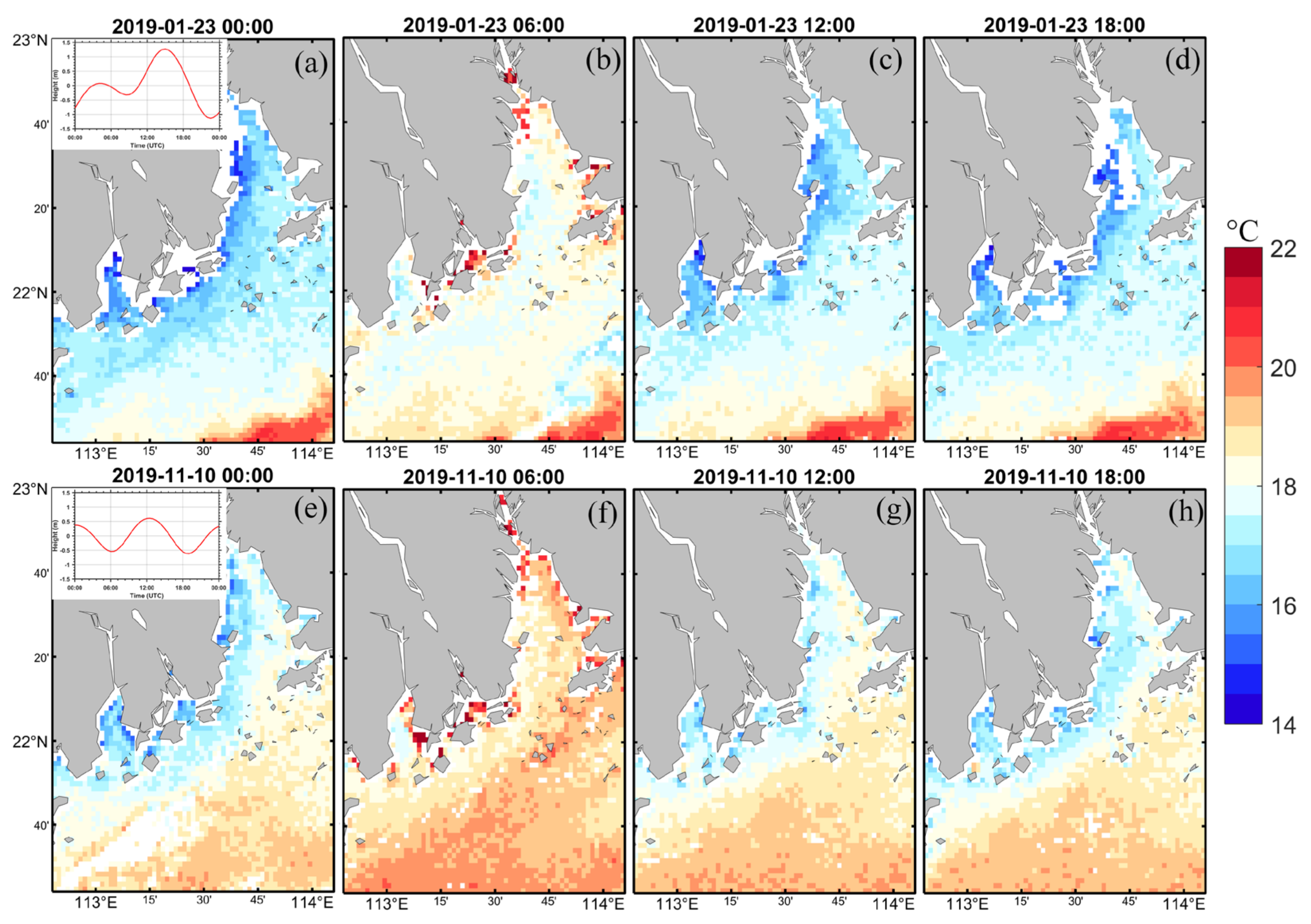
To set the stage for the discussion of the diurnal cycle in the thermal PR front occurrence, a description of diurnal SST variability in this study is warranted. Figure 2 shows several snapshots of 10-minutely SST for 23 January (spring tide) and 10 November 2019 (neap tide). The PR plume is very noticeable, with SST <16 °C for 23 January and <18 °C for 10 November. It is confined to shallow nearshore waters in the western PRE. The maximum SST contrast between onshore and offshore waters reaches about 8 °C. The SST on 23 January is much lower than on 10 November. On the other hand, the diurnal variability of SST in the PR plume is also more remarkable, relative to that for deep waters (>30 m). The two cases indicate that the spatially averaged SST in the plume zone increases about 2 °C from 00:00 to 06:00 UTC, and then gradually decreases to the initial level at 18:00 UTC.

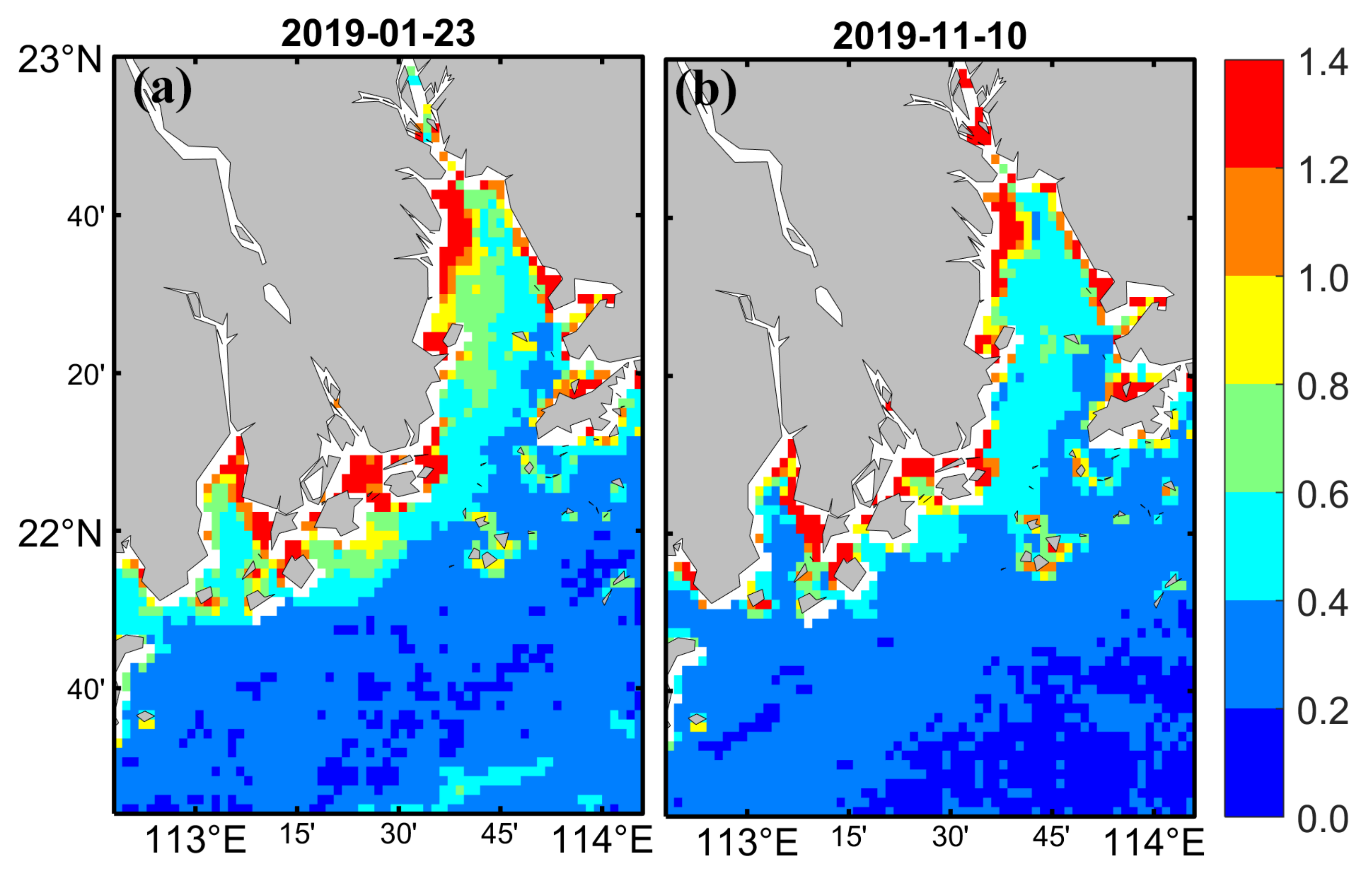
Figure 3 shows the SST standard deviations for the two days. They have similar patterns, with stronger amplitude along the western PR coast. The standard deviation decreases sharply with distance away from the coast. The standard deviation within the PR plume zone is >0.3 °C, with a maximum of 1.4 °C. In contrast, outside the plume, the SST standard deviation is much smaller. Overall, the relatively high standard deviation on 23 January extends seaward further than on 10 November, indicating larger changing range.

3.2. Diurnal Variability of the Pearl River Plume Front

To examine the spatial and temporal variability of the PRPF in more detail, we focus on the western region where the front is almost always persistent in winter.

3.2.1. Spatial Variability

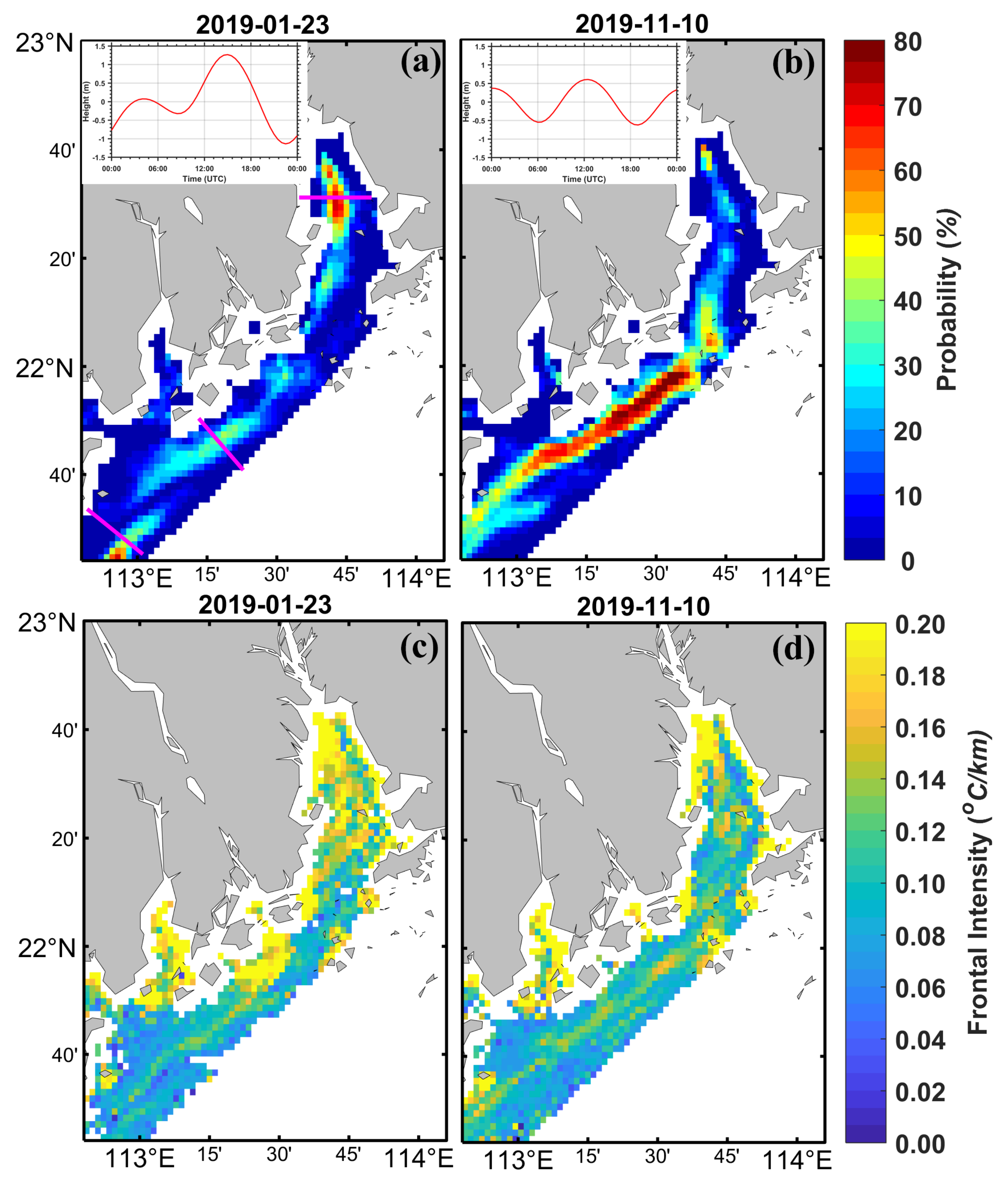
Figure 4 shows the frontal probability (upper) and mean GM images (bottom) by compositing 142 individual front images on 23 January (spring tide) and 10 November 2019 (neap tide). The distribution of the thermal plume front is nearly aligned to the coast and roughly follows the 5-m isobath, connecting cold, fresh water from the PR outflows with warm, saline water from offshore. It is equally evident that the thermal plume front is closer to the coast on 10 November. Due to spatial discontinuity of the plume front, we classify the plume front into three subfronts: the northern subfront north of 22° N 20′, the middle subfront between 22° N 20′ and 21° N 40′, and the southern subfront south of 21° N 40′. Each subfront shows discrepancy for the two cases. For the 23 January event, the northern and southern subfronts occur much more frequently (>60%) compared to that of the middle subfront (<45%). The mean frontal GM (Figure 4c) for the northern subfront (~0.2 °C/km) is the strongest while the weakest one is the southern subfront (~0.1 °C/km). For the 10 November event, the middle subfront has the highest probability (>70%) among the three (Figure 4b). The mean frontal GMs of the northern, middle, and southern subfronts are about 0.18, 0.13, and 0.16 °C/km, respectively (Figure 4d). These results indicate that the middle front on 23 January and the northern and southern subfronts on 10 November are highly variable.

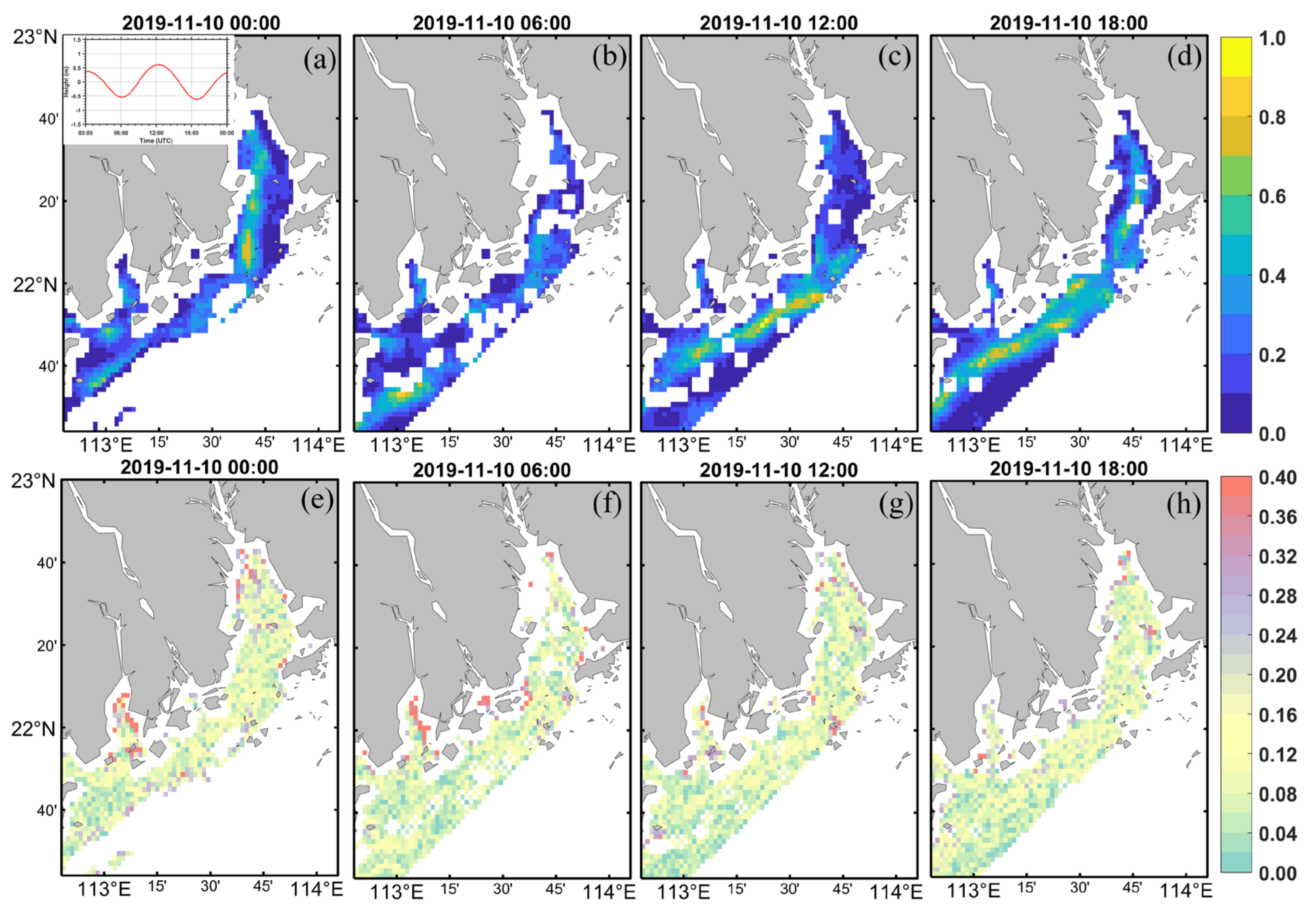
Figure 5 and Figure 6 show the spatial patterns of the 10-minutely JSDs and GMs for 23 January and 10 November 2019, respectively. The three plume subfronts (JS > 0.4) can be easily identified from the JSD snapshots (upper panel). Both JSDs and GMs indicate that the position and intensity of these subfronts exhibit strong variability at diurnal time scale. For the 23 January event, the positions for the northern, middle and southern subfronts tend to move northeastward, northwestward and southeastward, respectively. The maximum displacement is about 5 km from 00:00 to 18:00 UTC. On the other hand, the three subfronts are remarkable at 00:00 UTC. The northern and middle subfronts almost disappear at 06:00 UTC while the southern subfront becomes weak with a GM of ~0.12 °C/km. For the period of 12:00–18:00, the northern and middle subfronts gradually become strong again with a maximum GM of ~0.4 °C/km, while the southern subfront becomes weaker (~0.06 °C/km). For the 10 November event, diurnal variability differs considerably from that observed for the 23 January event. The positions of the three subfronts are closer to the coast. The northern subfront significantly oscillates in the east-west direction, with the maximum displacement of ~ 4 km and GM of ~ 0.35 °C/km. Nevertheless, the positions of the middle and southern subfronts show little variability. The corresponding maximum GMs reach about 0.2 and 0.3 °C/km, respectively.

3.2.2. Temporal Variability

To further explore the temporal variability of the thermal plume front quantitatively, three transects across the three subfronts are randomly selected (Figure 4a, in magenta color). The frontal intensity in terms of mean GM and the frontal position of the maximum JSD relative to an inshore point along the transects are calculated separately for each subfront.

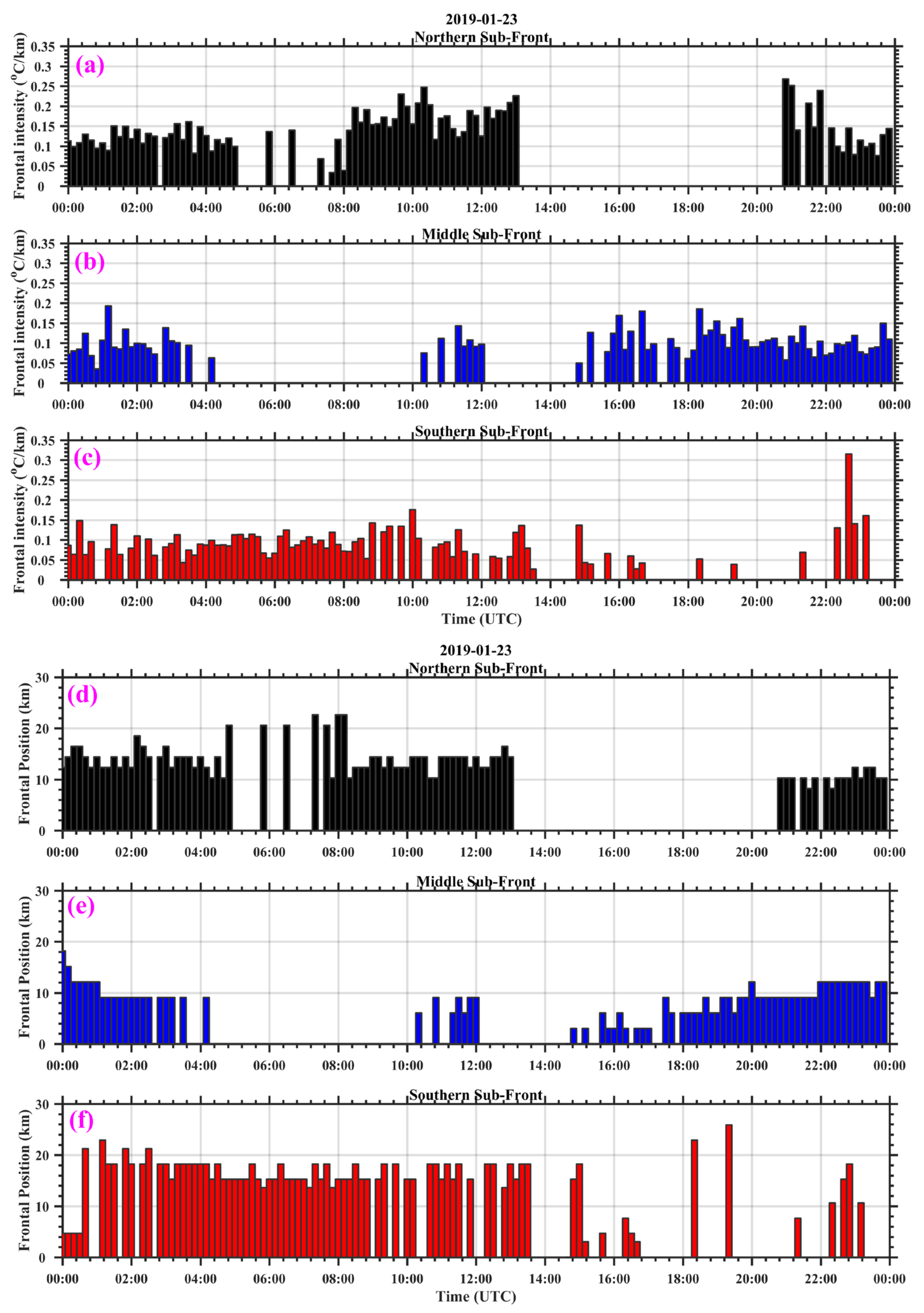
Figure 7 shows time series of the frontal intensity (a–c) and relative position (d–f) of the three subfronts for 23 January, which exhibits notable diurnal variability. The northern subfront (Figure 7a) remains weak intensity (GM < 0.15 °C/km) and sometimes disappears between 00:00 and 08:00 UTC when the frontal position tends to move offshore (Figure 7d). The frontal intensity then begins to increase, with the maximum spatially averaged intensity of about 0.26 °C/km. During this period, the subfront position has less variability. Between 22:00 and 24:00 UTC, the frontal intensity roughly decreases to the 00:00 UTC level, and the front moves towards onshore. The daily changing amplitudes in frontal intensity and position are about 0.05 °C/km and 7 km, respectively. There are no valid data approximately between 13:00 and 21:00 UTC due to cloud cover. For the middle subfront, the frontal intensity (Figure 7b) is averagely about 0.1 °C/km with a mean amplitude of 0.03 °C/km, while its position remains relatively stable (Figure 7e). A most noticeable feature is the disappearance of the subfront roughly between 04:00 and 10:00 UTC. For the southern subfront, the frontal intensity and position variability in general is less significant, though the subfront is intermittently absent between 14:00 and 24:00 UTC.

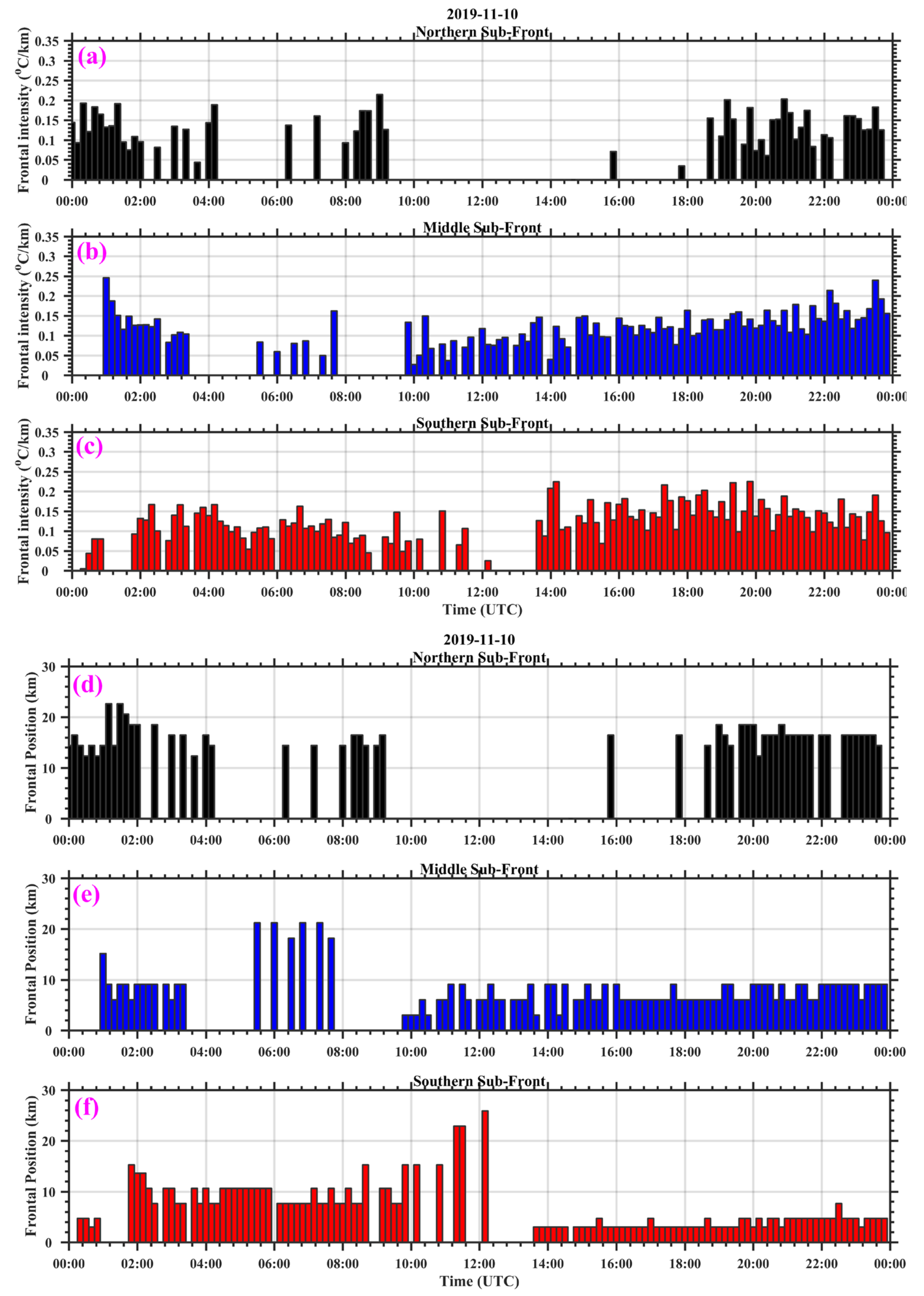
For the 10 November event (Figure 8), the frontal intensity in general exhibits strong-weak-strong fluctuations with the maximum amplitude of about 0.15 °C/km, while the frontal position tends to displace towards the coast, with a maximum displacement of about 15 km. For the three subfronts, the maximum diurnal variability is the middle subfront. Its intensity generally decreases between 01:00 and 10:00 UTC when the subfront displaces offshore (Figure 8b,e). The northern subfront has the lowest position variability (Figure 9d), the frontal intensity tends to decrease before 08:00, and is absent roughly between 09:00 and 19:00 UTC due to the front disappearance. Then, the subfront reproduces with an intensity of 0.15 °C/km (Figure 8a). For the southern subfront, the frontal intensity between 00:00 and 12:00 UTC is much weaker than between 14:00 and 24:00 UTC. The averaged GM ranges from 0.01 to 0.22 °C/km, with a mean amplitude of about 0.04 °C/km, while the averaged frontal position moves approximately 5 km towards the coast.

4. Discussion

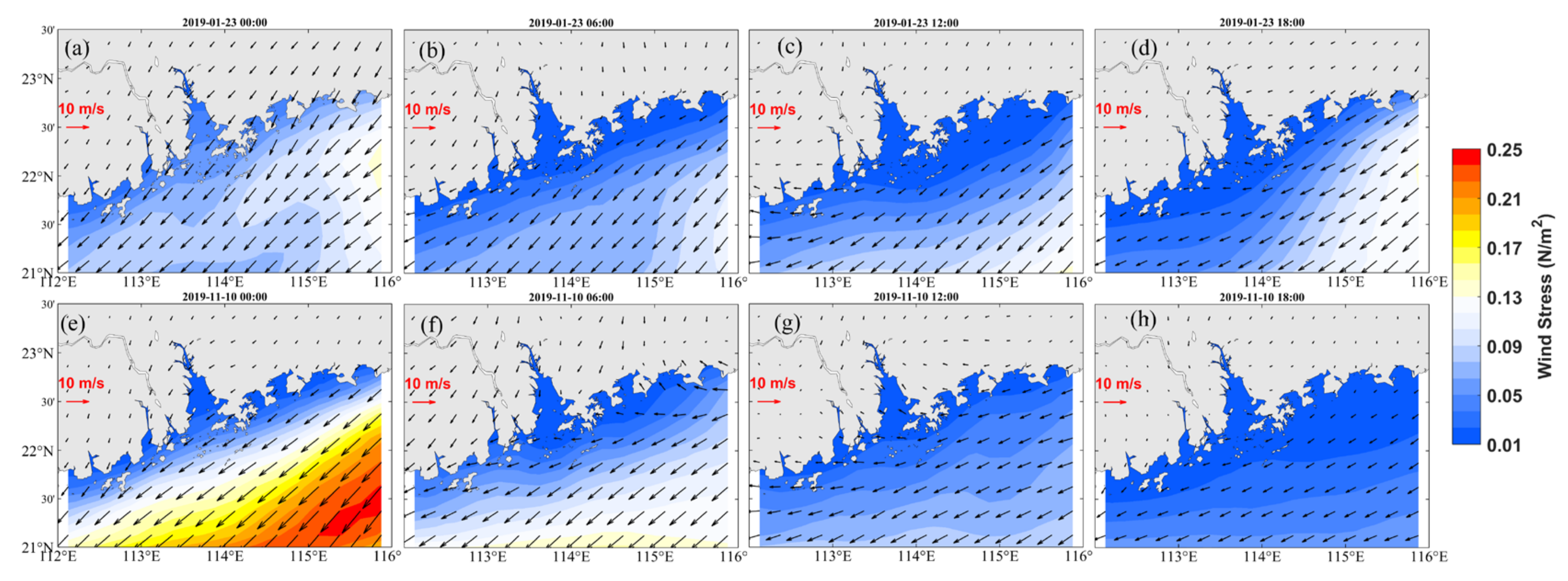
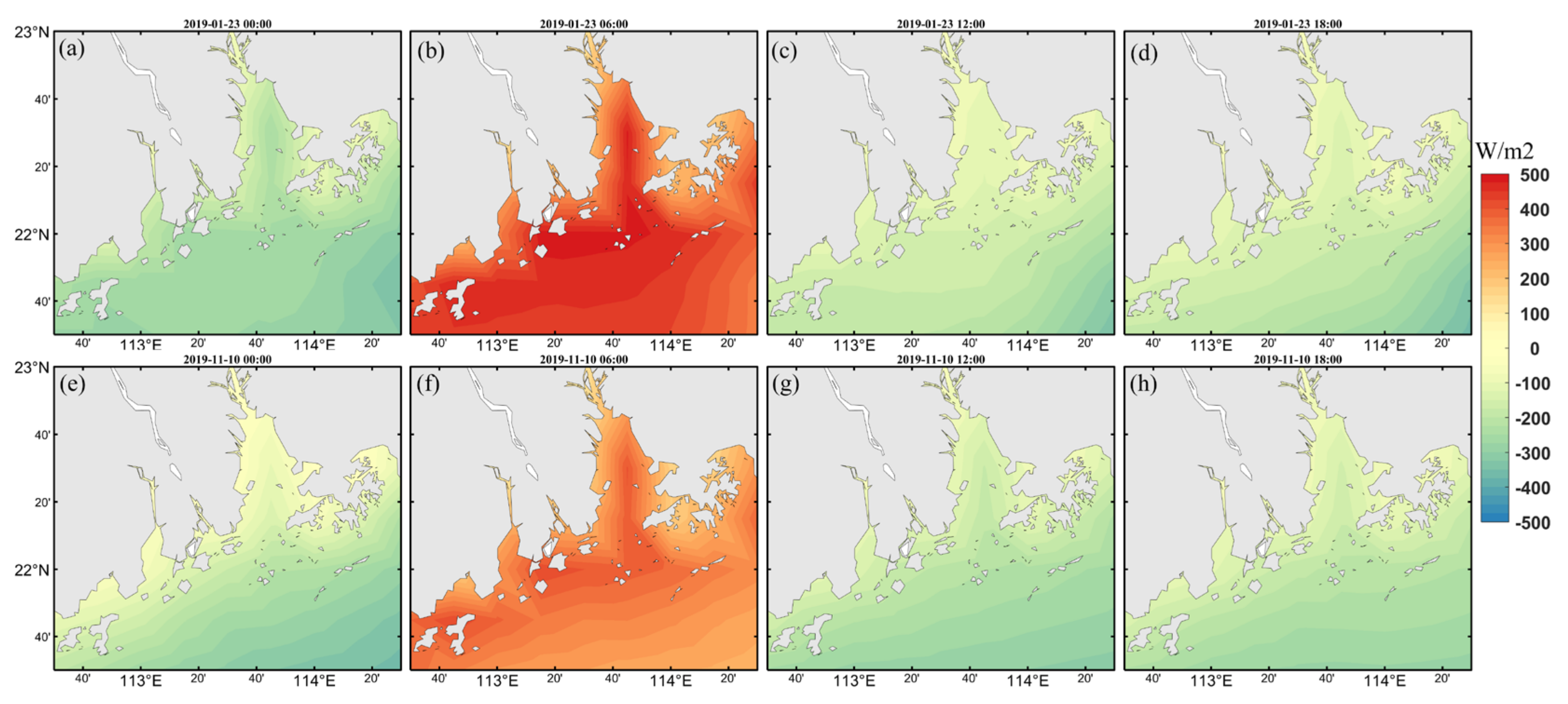
The satellite observations provide for the first time the diurnal variability of the thermal plume front associated with the PR outflow. A distinct feature for both spring and neap tides (Figure 5 and Figure 6) is that the plume front becomes less noticeable or even disappears at 06:00 UTC (14:00 in local time). Previous studies suggested that the plume is greatly controlled by river runoff, tide, and winds [24,33]. In addition, surface heating and cooling may be a contributing factor, as our study focuses on the thermal front. To see how the observed plume front can be accounted for by these factors. The six-hour surface winds and hourly net air-sea surface heat flux for the two cases are included for comparison. In this study, the runoff has very limited impact on the plume front variability, as it is well known that the river discharge remains stable in one day, especially during the dry season (October–May). We noted that the plume front experiences the flood-ebb tides for the 23 January event but is in the ebb tide for the 10 November event from 00:00 to 06:00 UTC when the plume frontal intensity gradually decreases for the two cases. This indicates that the tides cannot play a dominant role in the front variability at the hourly time scale. Figure 9 shows six-hour surface winds for the two events. The winds identically blow to the southwest and continue decreasing from 00:00 UTC, and the maximum speed around PRE region is less than 0.02 N/m². Figure 10 shows the corresponding snapshots of hourly air-sea net heat fluxes. Due to solar heating, the net air-sea surface heat flux increases significantly from 00:00 to 06:00 UTC, reaching maximum at 06:00 UTC (14:00, in local time) (Figure 10). In the situation, surface heating could result in faster heating of the thin fresh plume, thus decreasing the thermal contrast between the plume and the ambient shelf water and acting to weaken the front or even disappear.

The distinction of the front variability between the spring and neap tides is very remarkable. The plume front for the neap tide is generally closer to the coast while the frontal intensity is stronger, compared with those observed in the spring tide. This spring-neap variations in the frontal structure and position are supported by the detailed field measurements in Geyer [7], indicating that the plume front position shifts shoreward during neap tides of stronger stratification and moves seaward during spring tides of weaker stratification. Similar results are also found in numerical studies [28,34]. On the other hand, we noted that the northeasterly winds in neap tide are on average stronger than those in spring tide. Though the wind strength is much weak (<0.2 N/m²) for both events, it still may be possible to produce more onshore surface Ekman transport of warm coastal water for the 10 November event (neap tide), thereby enhancing the large SST difference between inshore and offshore water. This assumption is consistent to the findings of Zheng, Guan, Cai, Wei, and Huang [33], who indicated that the enhanced northeasterly winds are largely responsible for the westward movement of the plume front.

5. Conclusions

Using a robust edge-detection algorithm, the horizontal structure and diurnal variability of the wintertime PR thermal plume front during spring and neap tides are for the first time characterized from 10-min sequential SST images of Himawari-8 satellite observations. Our results indicate that the thermal plume front composes of three subfronts: the northern one north of 22° N 20′, the southern one south of 21° N 40′ and the middle one between them. The diurnal variability of the frontal intensity generally appears to be a strong-weak-strong pattern, with the weakest intensity observed at about 06:00 UTC. Further analysis suggests that the net surface heat flux over the region plays a dominant role in the frontal diurnal variability.

The comparison of diurnal variability of the thermal plume front between the spring and neap tides suggests that the front during the spring tide is more likely to be diffuse for the frontal structure, weak for the frontal intensity, and to move further seaward for the frontal position than those found during the neap tide. The significant differences may be largely attributed to the difference in tidally induced strong mixing during the spring tide, while the wind stress difference is probably a secondary controlling factor.

The Himawari-8 satellite remote sensing only provides information about skin surface temperature signature. The PR plume in winter is marked by colder and fresher than the offshore water, the surface thermal front normally coincides with the salinity front [24]. It is however not possible to tell if the subsurface thermal plume front has the same varying patterns. In other seasons when the plume is mostly characterized by strong salinity gradients, SST contrast on two sides of the plume front is more obscure. It is also not possible to directly relate the thermal front to the plume front. To better understand high-frequency variability of the plume front under different environmental conditions, future studies may attempt to complement the satellite-derived thermal fronts with multiple ocean color satellite observations and subsurface in situ data.

References

- Fedorov, K.N. The Physical Nature and Structure of Oceanic Fronts; Springer: New York, NY, USA, 1986. [Google Scholar]
- Ou, H.W.; Dong, C.M.; Chen, D. Tidal diffusivity: A mechanism for frontogenesis. J. Phys. Oceanogr. 2003, 33, 840–847. [Google Scholar] [CrossRef] [Green Version]
- Orton, P.M.; Jay, D.A. Observations at the tidal plume front of a high-volume river outflow. Geophys. Res. Lett. 2005, 32, 1–16. [Google Scholar] [CrossRef] [Green Version]
- Taylor, J.R.; Ferrari, R. Ocean fronts trigger high latitude phytoplankton blooms. Geophys. Res. Lett. 2011, 38, L23601. [Google Scholar] [CrossRef]
- Yuan, D.L.; Qiao, F.L.; Su, J. Cross-shelf penetrating fronts off the southeast coast of China observed by MODIS. Geophys. Res. Lett. 2005, 32, L19603. [Google Scholar] [CrossRef]
- Belkin, I.M.; Cornillon, P.C.; Sherman, K. Fronts in Large Marine Ecosystems. Prog. Oceanogr. 2009, 81, 223–236. [Google Scholar] [CrossRef]
- Geyer, W.R. Tide-induced mixing in the Amazon Frontal Zone. J. Geophys. Res. Ocean. 1995, 100, 2341–2353. [Google Scholar] [CrossRef]
- Guo, L.; Xiu, P.; Chai, F.; Xue, H.; Wang, D.; Sun, J. Enhanced Chlorophyll Concentrations Induced by Kuroshio Intrusion Fronts in the Northern South China Sea. Geophys. Res. Lett. 2017, 44, 11565–11572. [Google Scholar] [CrossRef] [Green Version]
- Cotroneo, Y.; Budillon, G.; Fusco, G.; Spezie, G. Cold core eddies and fronts of the Antarctic Circumpolar Current south of New Zealand from in situ and satellite data. J. Geophys. Res. Ocean. 2013, 118, 2653–2666. [Google Scholar] [CrossRef]
- Miller, P.I. Detection and visualisation of oceanic fronts from satellite data, with applications for fisheries, marine megafauna and marine protected areas. In Handbook of Satellite Remote Sensing Image Interpretation: Applications for Marine Living Resources Conservation and Management; EU PRESPO and IOCCG: Dartmouth, NS, Canada, 2011; pp. 229–239. [Google Scholar]
- Mendes, R.; Vaz, N.; Fernández-Nóvoa, D.; da Silva, J.C.B.; de Castro, M.; Gómez-Gesteira, M.; Dias, J.M. Observation of a turbid plume using MODIS imagery: The case of Douro estuary (Portugal). Remote Sens. Environ. 2014, 154, 127–138. [Google Scholar] [CrossRef]
- Saldías, G.S.; Sobarzo, M.; Largier, J.; Moffat, C.; Letelier, R. Seasonal variability of turbid river plumes off central Chile based on high-resolution MODIS imagery. Remote Sens. Environ. 2012, 123, 220–233. [Google Scholar] [CrossRef]
- He, S.; Huang, D.; Zeng, D. Double SST fronts observed from MODIS data in the East China Sea off the Zhejiang-Fujian coast, China. J. Mar. Syst. 2015, 154, 93–102. [Google Scholar] [CrossRef]
- Zhang, Y.; Zeng, L.; Wang, Q.; Geng, B.; Liu, C.; Shi, R.; Liu, N.; Wang, W.; Wang, D. Seasonal variation in the three-dimensional structures of coastal thermal front off western Guangdong. Acta Oceanol. Sin. 2021, 40, 88–99. [Google Scholar] [CrossRef]
- Pisoni, J.P.; Rivas, A.L.; Piola, A.R. On the variability of tidal fronts on a macrotidal continental shelf, Northern Patagonia, Argentina. Deep. Sea Res. Part II Top. Stud. Oceanogr. 2014, 119, 61–68. [Google Scholar] [CrossRef]
- Ren, S.H.; Xie, J.P.; Zhu, J. The Roles of Different Mechanisms Related to the Tide-induced Fronts in the Yellow Sea in Summer. Adv. Atmos. Sci. 2014, 31, 1079–1089. [Google Scholar] [CrossRef]
- Jing, Z.; Qi, Y.; Fox-Kemper, B.; Du, Y.; Lian, S. Seasonal thermal fronts on the northern South China Sea shelf: Satellite measurements and three repeated field surveys. J. Geophys. Res. Ocean. 2016, 121, 1914–1930. [Google Scholar] [CrossRef] [Green Version]
- Wang, Y.; Yu, Y.; Zhang, Y.; Zhang, H.R.; Chai, F. Distribution and variability of sea surface temperature fronts in the south China sea. Estuar. Coast. Shelf Sci. 2020, 240, 106793. [Google Scholar] [CrossRef]
- Kahru, M.; Di Lorenzo, E.; Manzano-Sarabia, M.; Mitchell, B.G. Spatial and temporal statistics of sea surface temperature and chlorophyll fronts in the California Current. J. Plankton Res. 2012, 34, 749–760. [Google Scholar] [CrossRef] [Green Version]
- Castelao, R.M.; Wang, Y. Wind-driven variability in sea surface temperature front distribution in the California Current System. J. Geophys. Res. Ocean. 2014, 119, 1861–1875. [Google Scholar] [CrossRef]
- Wang, D.X.; Liu, Y.; Qi, Y.Q.; Shi, P. Seasonal variability of thermal fronts in the northern South China Sea from satellite data. Geophys. Res. Lett. 2001, 28, 3963–3966. [Google Scholar] [CrossRef]
- Chang, Y.; Shimada, T.; Lee, M.-A.; Lu, H.-J.; Sakaida, F.; Kawamura, H. Wintertime sea surface temperature fronts in the Taiwan Strait. Geophys. Res. Lett. 2006, 33, L23603. [Google Scholar] [CrossRef]
- Chang, Y.; Shieh, W.-J.; Lee, M.-A.; Chan, J.-W.; Lan, K.-W.; Weng, J.-S. Fine-scale sea surface temperature fronts in wintertime in the northern South China Sea. Int. J. Remote Sens. 2010, 31, 4807–4818. [Google Scholar] [CrossRef]
- Lai, Z.; Ma, R.; Gao, G.; Chen, C.; Beardsley, R.C. Impact of multichannel river network on the plume dynamics in the Pearl River estuary. J. Geophys. Res. Ocean. 2015, 120, 5766–5789. [Google Scholar] [CrossRef] [Green Version]
- Yu, Y.; Zhang, H.-R.; Jin, J.; Wang, Y. Trends of sea surface temperature and sea surface temperature fronts in the South China Sea during 2003–2017. Acta Oceanol. Sin. 2019, 38, 106–115. [Google Scholar] [CrossRef]
- Bessho, K.; Date, K.; Hayashi, M.; Ikeda, A.; Imai, T.; Inoue, H.; Kumagai, Y.; Miyakawa, T.; Murata, H.; Ohno, T.; et al. An introduction to Himawari-8/9—Japan’s new-generation geostationary meteorological satellites. J. Meteorol. Soc. Japan. Ser. II 2016, 94, 151–183. [Google Scholar] [CrossRef] [Green Version]
- Mao, Q.; Shi, P.; Yin, K.; Gan, J.; Qi, Y. Tides and tidal currents in the Pearl River Estuary. Cont. Shelf Res. 2004, 24, 1797–1808. [Google Scholar] [CrossRef]
- Lai, Z.; Ma, R.; Huang, M.; Chen, C.; Chen, Y.; Xie, C.; Beardsley, R.C. Downwelling wind, tides, and estuarine plume dynamics. J. Geophys. Res. Ocean. 2016, 121, 4245–4263. [Google Scholar] [CrossRef] [Green Version]
- Kurihara, Y.; Murakami, H.; Kachi, M. Sea surface temperature from the new Japanese geostationary meteorological Himawari-8 satellite. Geophys. Res. Lett. 2016, 43, 1234–1240. [Google Scholar] [CrossRef] [Green Version]
- Egbert, G.D.; Erofeeva, S.Y. Efficient Inverse Modeling of Barotropic Ocean Tides. J. Atmos. Ocean. Technol. 2002, 19, 183–204. [Google Scholar] [CrossRef] [Green Version]
- Shimada, T.; Sakaida, F.; Kawamura, H.; Okumura, T. Application of an edge detection method to satellite images for distinguishing sea surface temperature fronts near the Japanese coast. Remote. Sens. Environ. 2005, 98, 21–34. [Google Scholar] [CrossRef]
- Chang, Y.; Cornillon, P. A comparison of satellite-derived sea surface temperature fronts using two edge detection algorithms. Deep. Sea Res. Part II Top. Stud. Oceanogr. 2015, 119, 40–47. [Google Scholar] [CrossRef] [Green Version]
- Zheng, S.; Guan, W.; Cai, S.; Wei, X.; Huang, D. A model study of the effects of river discharges and interannual variation of winds on the plume front in winter in Pearl River Estuary. Cont. Shelf Res. 2014, 73, 31–40. [Google Scholar] [CrossRef]
- Li, M.; Zhong, L. Flood–ebb and spring–neap variations of mixing, stratification and circulation in Chesapeake Bay. Cont. Shelf Res. 2009, 29, 4–14. [Google Scholar] [CrossRef]
Figure 1.
Bathymetry of Pearl River and adjacent coastal region. Gray contours indicate isobaths (in meter). A tide gauge site is marked by bule solid triangle. Area map is shown in upper-left corner.
Figure 2.
Ten-minutely sea surface temperature (SST) on 23 January (a–d) and 10 November 2019 (e–f). Corresponding tidal heights are shown in upper-left corners of (a,e). The subtitles in subplots (a–h) indicate the corresponding observation time (unit: UTC).
Figure 3.
SST standard deviations for 23 January (a) and 10 November 2019 (b).
Figure 4.
Ten-minutely frontal probability (unit: %, a,b) and mean frontal intensity (unit: °C/km, c,d) for 23 January (a) and 10 November 2019 (b). Magenta color lines in (a) denote three transects across the front. Corresponding tidal heights are shown in upper-left corners of (a,b).
Figure 5.
Spatial patterns of 10-minutely frontal intensity represented by both Jensen–Shannon divergence (JSD) (a–d) and gradient magnitude (GM) (e–h) on 23 January 2019. Corresponding tidal height is shown in upper-left corner of (a). The subtitles in subplots (a–h) indicate the corresponding observation time (unit: UTC).
Figure 6.
Same as Figure 5, but for 10 November 2019.
Figure 7.
Time series of spatially averaged GMs (a–c); frontal positions of maximum JS frontal values (d–f) across three transects (Figure 4a) for 23 January 2019.
Figure 8.
Same as Figure 7, but for 10 November 2019.
Figure 9.
Six-hourly surface winds overlaid with wind stress (color shading) for 23 January (a–d) and 10 November 2019 (e–h). The subtitles in subplots (a–h) indicate the corresponding observation time (unit: UTC).
Figure 10.
Six snapshots of hourly air-sea net heat fluxes for 23 January (a–d) and 10 November 2019 (e–h). Positive values represent seawater net heat gain. The subtitles in subplots (a–h) indicate the corresponding observation time (unit: UTC).
Publisher’s Note: MDPI stays neutral with regard to jurisdictional claims in published maps and institutional affiliations. |
© 2021 by the authors. Licensee MDPI, Basel, Switzerland. This article is an open access article distributed under the terms and conditions of the Creative Commons Attribution (CC BY) license (https://creativecommons.org/licenses/by/4.0/).
Share and Cite
MDPI and ACS Style
Hu, Z.; Xie, G.; Zhao, J.; Lei, Y.; Xie, J.; Pang, W. Mapping Diurnal Variability of the Wintertime Pearl River Plume Front from Himawari-8 Geostationary Satellite Observations. Water 2022, 14, 43. https://doi.org/10.3390/w14010043
AMA Style
Hu Z, Xie G, Zhao J, Lei Y, Xie J, Pang W. Mapping Diurnal Variability of the Wintertime Pearl River Plume Front from Himawari-8 Geostationary Satellite Observations. Water. 2022; 14(1):43. https://doi.org/10.3390/w14010043
Chicago/Turabian StyleHu, Zifeng, Guanghao Xie, Jun Zhao, Yaping Lei, Jinchi Xie, and Wenhong Pang. 2022. "Mapping Diurnal Variability of the Wintertime Pearl River Plume Front from Himawari-8 Geostationary Satellite Observations" Water 14, no. 1: 43. https://doi.org/10.3390/w14010043
Note that from the first issue of 2016, this journal uses article numbers instead of page numbers. See further details here.