
Environmental Background Values and Ecological Risk Assessment of Heavy Metals in Watershed Sediments: A Comparison of Assessment Methods

Center for Eco-Environmental Engineering, Dongguan University of Technology, Dongguan 523808, China
*
Author to whom correspondence should be addressed.
Water 2022, 14(1), 51; https://doi.org/10.3390/w14010051
Submission received: 23 November 2021
/
Revised: 18 December 2021
/
Accepted: 20 December 2021
/
Published: 27 December 2021
(This article belongs to the Special Issue New Insights on Pollution and Remediation of Trace Elements in Coastal and Estuarine Sediments)
Abstract
:The distribution and assessment of heavy metal pollution in sediments have been extensively studied worldwide. Risk assessment methods based on total content, background values, and sediment quality guidelines are widely applied but have never been compared. We systematically sorted out these evaluation methods, obtained evaluation results using actual monitoring data, and compared their applicability. The results showed that the background values of different metals are significantly different, which may depend on their mobility. Geoaccumulation index (Igeo) and enrichment factor (EF) values invariably decreased with the increase of background values for individual heavy metal enrichment risk assessment. Compared with EF, Igeo also showed a significant positive linear correlation with heavy metal content. Pollution load index (PLI), modified contamination degree (mCd), and potential ecological risk index (RI) showed significant differences in response to background values and evaluation levels for the comprehensive risk of heavy metal enrichment, but their distribution trends along with the sampling points were basically identical. Toxic risk index (TRI), mean ERM quotient (mERMQ), and contamination severity index (CSI) were used to evaluate the damage degree of complex heavy metals to aquatic organisms and shared a similar whole-process distribution trend. The modified hazard quotient (mHQ), which is used to evaluate the toxicity of a single heavy metal to aquatic organisms, showed a significant positive linear correlation with the total content of each heavy metal, indicating that the toxic effect on organisms can be predicted through the direct monitoring. The results of this study have important guiding significance for the selection of evaluation methods for heavy metal pollution in sediments.
1. Introduction
As one of the main pollutants in the water environment, heavy metals have raised concern regarding their effect on water ecosystem safety and human health. Heavy metals in water can migrate into sediments through physical, chemical, and biological reactions [1,2]. Meanwhile, heavy metals in sediments will be released upward with the change of environmental conditions, causing secondary pollution of the water environment [3]. The content of heavy metals in sediments is usually three to six orders of magnitude higher than that in water, which implies that sediment is the main storage reservoir of heavy metals in water environment and plays an important indicator role for water pollution [3,4]. Currently, various indexes have been developed to assess environmental risks for heavy metals in sediments based on their total contents, bioavailability, and toxicity [5,6,7]. Although many researches have highlighted that the morphological content can well reveal the migration and toxicity of heavy metals in sediments, total content can directly reflect the degree and source of contamination [8,9]. Therefore, risk assessment based on total concentration calculation remains an indispensable method in the study of heavy metal pollution in water environment and a key pathway to identify pollution sources.
Heavy metal risk assessment methods based on total concentration calculation have been widely proposed [10,11], mainly including two categories: one is related to background values, the other is related to sediment quality guidelines. Background values mainly include three types: soil background value in each investigated area (Bv), control value of surface sediment (Cvs, samples collected from the study area that are uncontaminated), and control value of deep sediment (Cvd, samples collected from the bottom of sedimentary column). However, the selection of background values in previous studies was not uniform, resulting in large differences in evaluation results and low comparability.
Sediment quality guidelines (SQGs) are the actual allowable values of a specific chemical substance in sediments that does not harm benthic aquatic organisms or other relevant water functions [7,12]. Although there is still no internationally agreed methodology, the SQGs have been useful in numerous applications, such as designing monitoring programs, interpreting historical data, ecological risk assessment, and developing sediment quality remediation objectives [13]. The current SQGs are mainly derived from various states in North America for both freshwater and marine ecosystems and are composed of a variety of calculations [14]. However, few studies have concentrated on the comparison of different methods, which may lead to the possible confusion of these evaluation indicators.
The pollution assessment method compares the concentration of heavy metals with background values and SQGs, which helps to evaluate the accumulation of heavy metals in sediments. Thus, it is essential to consider the intensity of metal pollution by inventorying the concentrations and their distribution in a riverine ecosystem. In addition, the various bases of assessment indices predict inconsistent risks of heavy metals in sediments of different regions [5]. In order to avoid biases in the risk assessment of heavy metals in sediments, a combination of different indicators should be used. However, the existing researches mainly focus on the superposition application of each single method [7,10] and thus lack mutual comparison, leading to confusion, especially when the effects of background values and SQGs have not been highlighted.
Therefore, we assume that each assessment method is sufficiently independent, and that the distribution and migration of heavy metals are mainly affected by pollution sources and environmental factors, so the risk of heavy metals depends on the content of heavy metals and background values. This study comprehensively compared and analyzed various evaluation methods based on the calculation of actual detection data, aiming to reveal the importance of the selection of evaluation methods, background values and SQGs. The main objectives were (a) to analyze the vertical distribution of heavy metals in sediments and to obtain three types of background values, (b) to compare the results of selected evaluation methods with the application of background values, and (c) to reveal the relationship between evaluation methods and background values and SQGs.
2. Materials and Methods
2.1. Study Area and Data Source
The Beijiang River is situated in Guangdong Province, China, and flows through Shaoguan City, Yingde City, Qingyuan City, and Foshan City from upstream to downstream, and then converges in the Pearl River Estuary. It is a major source of drinking water and an ecological safety barrier in Guangdong Province. With the adjustment of Guangdong’s industrial layout, a large number of small- and medium-sized enterprises, taking advantage of the “golden waterway”, move to the cities along the Beijiang River. The development of cement, ceramics, smelting, and other manufacturing industries has led to the continuous deterioration of water quality of the Beijiang River, which poses a serious threat to regional ecological and environmental security [15,16]. The data of this study were derived from the sampling survey of sediments throughout the Beijiang River. In April 2018, 23 columnar sediment samples were collected by drilling. The depth of each sample column was 3 m and was divided into 9 sections: 0–0.2 m, 0.2–0.4 m, 0.4–0.6 m, 0.6–0.8 m, 0.8–1.0 m, 1.0–1.5 m, 1.5–2.0 m, 2.0–2.5 m, and 2.5–3.0 m, respectively. Each part of the intercepted sediment sample was thoroughly mixed, and three small portions were taken out for pretreatment, such as drying, grinding, and digestion. After volumetric determination, heavy metals, Cr, Ni, Cu, Zn, As, Cd, Tl, Pb, and Hg, as well as common metallic element Fe were measured by atomic absorption spectrometry. The detailed detection methods and quality assurance were shown in a previous study [17]. Moreover, in order to obtain control values of surface sediments suitable to the actual environment, three samples were collected from tributaries nearby that were not affected by point sources.
In particular, the data here were used only to analyze vertical distribution trends, with the purpose of obtaining control values for deep sediments, rather than analyzing pollution mechanisms. On the basis of obtaining background values, we uniformly used the total concentration data of heavy metals in the surface layer of 0–0.2 m to conduct pollution assessment and focused on analyzing the differences in the results obtained by different types of assessment methods.
2.2. Assessment Methods
The selected evaluation methods are all calculated based on total concentrations of heavy metals, background values and SQGs, which are introduced as follows.
2.2.1. Geoaccumulation Index (Igeo)
The geoaccumulation index (Igeo) has been widely used in the assessment of heavy metal pollution and reveals the relationship between heavy metals in sediments and geochemical background values, which was originally proposed by Muller [18]. The Igeo value is defined as
where Cn represents the measured concentration of metal (n) (mg/kg), Bn represents the geochemical background value of metal (n) (mg/kg), and 1.5 is a factor used to minimize the impact of background value caused by lithological variation [19]. The Igeo consists of 7 levels, as shown in Table S1.
2.2.2. Enrichment Factor (EF)
Enrichment factor (EF) is considered to be an effective tool to evaluate the enrichment of pollutants in the environment. To ascertain the impact of anthropogenic activities on sediment, the measured heavy metal concentrations are compared with conservative elements (such as Al and Fe) that are not affected by weathering [20,21]. Here, Fe is selected as the conservative metal, and the EF value is defined as
where (Cn/CFe)sample represents the ratio between the measured heavy metal concentration and Fe concentration in the contaminated sediment sample, and (Bn/BFe)background represents the ratio between the measured heavy metal concentration and Fe concentration in the background sediment sample. EF > 1.5 indicates that heavy metals are derived from anthropogenic origin, while EF < 1.5 indicates that heavy metals are completely derived from natural weathering [22]. The EF consists of 7 levels, as shown in Table S2.
2.2.3. Contamination Factor (Cf) and Pollution Load Index (PLI)
Contamination factor (Cf) is used to show the contamination degree with a single metal and is the ratio of the content of each metal to its background value. Pollution load index (PLI) is an empirical index which provides a simple and comparative means for assessing metal pollution levels and is a geometric evaluation of the individual Cf [23]. The calculation methods of Cf and PLI are as follows:
where Cn is the measured concentration of the target heavy metal (mg/kg), Bn is the selected background concentration of the target heavy metal (mg/kg), and n is the quantity of the target heavy metal. The recommended pollution levels for PLI classification are as follows: no pollution (PLI ≤ 1) and polluted (PLI > 1) [24].
2.2.4. Modified Contamination Degree (mCd)
Contamination degree (Cd) is defined as the sum of all contamination factors (Cf). As it is not always feasible to analyze all the components used in this indicator, Abrahim and Parker proposed an improved method, which was defined as modified contamination degree (mCd) [25], and it was calculated as
where Cfi represents the contamination factor, and n represents the number of target heavy metals. The classifications of contamination levels are shown in Table S3.
2.2.5. Potential Ecological Risk Index (RI)
Potential ecological risk of individual factor (Eri) and potential ecological risk index (RI) were proposed by Hakanson to determine the ecological impact and potential risk of heavy metals exposure [23]. It illustrates ecological sensitivity and vulnerability towards toxic heavy metals and evaluates the comprehensive ecological risk. Four factors are considered: the type of target heavy metals, measured concentration, toxicity coefficient, and sensitivity of water body to heavy metals. The equation is
where Cfi represents the contamination factor, and n represents the number of target heavy metals. Tri represents the toxicity coefficient of a single heavy metal [6], and the toxicity coefficients of target heavy metals are shown in Table S4. The classifications of ecological risk levels are shown in Table S5.
2.2.6. Toxic Risk Index (TRI)
Toxic risk index (TRIi) is known as a newly validated method for evaluating the ecotoxicity of system in view of the TEL (threshold effect level) and PEL (probable effect level) effects, which is applied to normalize the toxicities caused by different heavy metals and then facilitated the comparison of their relative effects [26]. The TEL and PEL values of target heavy metals are shown in Table S4. The potential acute toxicity of the heavy metals in a sediment sample can be assessed as the sum of TRIi. The TRIi and TRI can be calculated as
where Ci represents the measured concentration of heavy metal i, and n represents the number of target heavy metals, TELi is the TEL value of the target heavy metal i, and PELi is the PEL value of the target heavy metal i. The pollution levels of the TRI are classified as shown in Table S6.
2.2.7. Modified Hazard Quotient (mHQ)
The modified hazard quotient (mHQ) is used to evaluate sediment contamination by comparing heavy metal contents in the sediment with effect level standards (PEL, SEL (severe effect level), and TEL) [27]. It is considered a significant tool because it exemplifies the extent of risk each heavy metal poses to the biota and aquatic habitat [7]. TEL, PEL, and SEL values of target heavy metals are shown in Table S4. The mHQ is evaluated following the mathematical expression below:
where Ci represents the measured concentration of heavy metal i, TELi is the TEL value of the target heavy metal i, PELi is the PEL value of the target heavy metal i, and SELi is the SEL value of the target heavy metal i. The contamination levels of the mHQ are classified as shown in Table S7.
2.2.8. Mean ERM Quotient (mERMQ)
Mean ERM quotient (mERMQ) is proposed for assessing the potential effects of multiple heavy metal contamination in sediment. The sediment quality guidelines were developed from biological toxicity test of the benthic environment and classified into three levels by ERL (effect range low) and ERM (effect range medium) as rarely (<ERL), occasionally (ERL-ERM), or frequently (≥ERM) associated with adverse biological effects [28,29]. ERL and ERM values of target heavy metals are shown in Table S4. The mERMQ is calculated as follows:
where mERMQ is the effect-range median quotient of multiple metal contamination, ERMQi is the effect-range quotient of heavy metal i, Ci is the measured content of the target heavy metal i, ERMi is the ERM value of the target heavy metal i, and n is the number of metals. The contamination levels of mERMQ are classified as shown in Table S8.
2.2.9. Contamination Severity Index (CSI)
The contamination severity index (CSI) is a new index based on ERL and ERM values to study the severity of heavy metal contamination in sediments, which was first proposed by Pejman [30], for the toxicity boundaries and adverse effect on the biota as well as weighted values for each heavy metal attributed by the ratio of the PCA/FA as site-specific factor [6]. The CSI is calculated as follows:
where wi is the weight of the heavy metal i, Ci is the measured content of the target heavy metal i, ERLi is the ERL value of the target heavy metal i, ERMi is the ERM value of the target heavy metal i, and n is the number of selected metals. The pollution levels of the CSI are classified as shown in Table S9.
The ratio PCA/FA is used to obtain the weight (wi) of each heavy metal. This method only considered the factors with human influence to calculate the weighted value. The weight of each heavy metal is calculated as follows:
2.3. Statistical Analysis
All statistical analyses were performed using SPSS 19.0 software packages. Results were expressed as mean ± standard deviation. Differences were considered significant when p < 0.05. Principal component analysis (PCA) and factor analysis (FA) were performed to analyze the occurrence relationship between heavy metals to obtain the weight value wi.
3. Results and Discussion
3.1. Vertical Distribution and Background Values of Heavy Metals
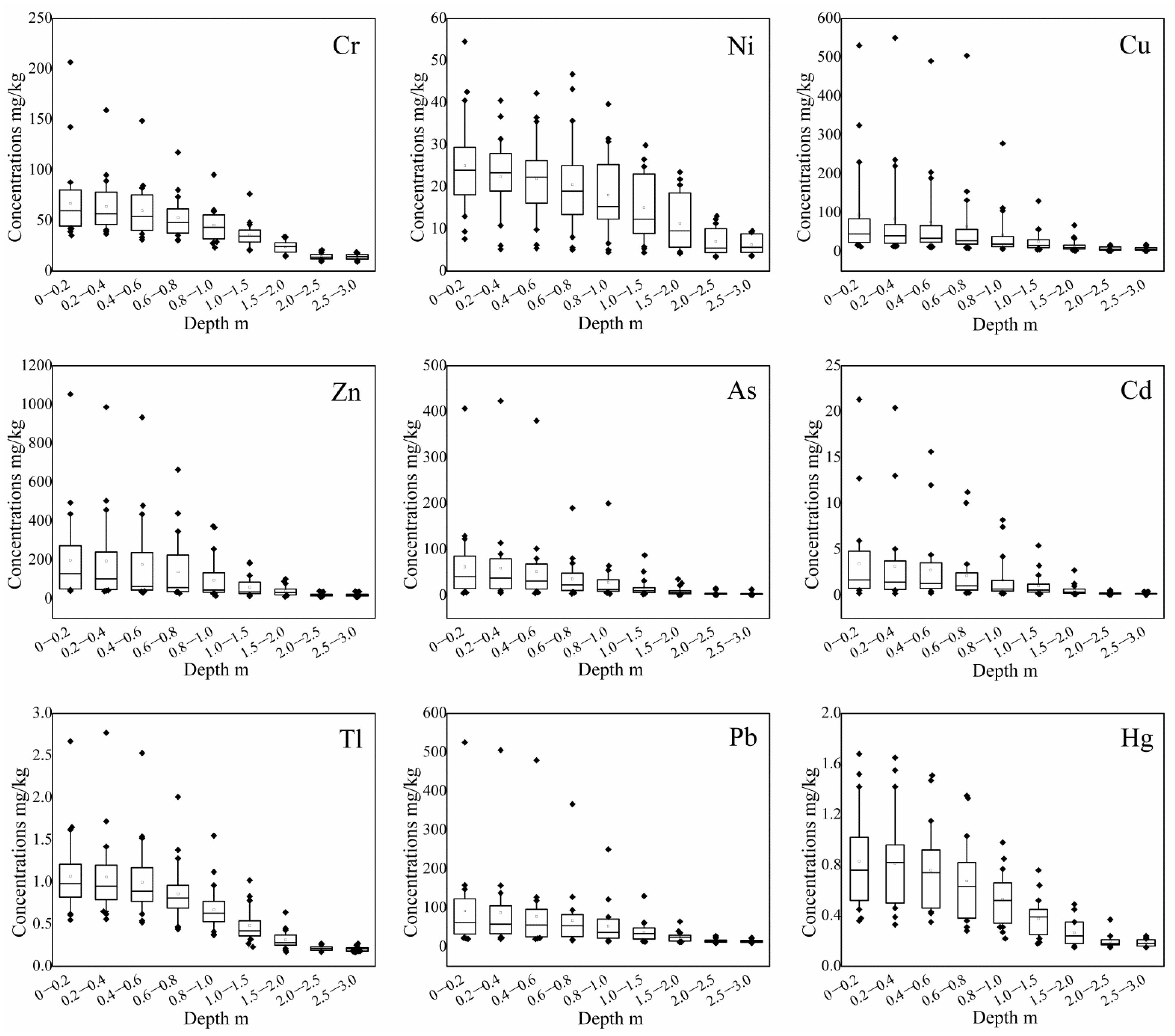
Figure 1 illustrates the concentration distribution of Cr, Ni, Cu, Zn, As, Cd, Tl, Pb, and Hg with depth in sediment cores from 23 sampling sites along the Beijiang River. Except for Ni and Cu, all other heavy metals fluctuated in the depth range of 0–0.6 m and showed a slightly decreasing trend. The results are comparable to those of previous studies, suggesting that the large fluctuation of heavy metals in surface sediments is mainly caused by human activities and hydraulic disturbance [31,32,33]. Given the prevalence of diagenesis, heavy metal concentrations declined rapidly in the subsequent depth of 0.6–2.5 m, indicating that heavy metals were gradually deposited into deep sediments under the action of sediment adsorption and gravity [34,35]. However, the deposition rate decreased with the increase of depth, and the rate of different metals varied slightly. After 2.5 m, heavy metal concentrations basically remained stable, indicating that sediments beyond this depth were barely disturbed by human activities and the diagenesis also decreased, which can be verified by isotope dating [36,37]. Therefore, the heavy metal concentrations in subsequent deep sediments can be defined as background values, which are defined as the deep control values (Cvd).
As a conservative metal element, the content of Fe is not affected by weathering and is significantly related to the distribution of heavy metals, which can effectively reflect the accumulation of heavy metals in sediments caused by human activities [4,7]. As shown in Figure S1, the distribution trend of Fe was basically consistent with that of the target heavy metals, which can be used to interpret the enrichment of heavy metals. In addition, we collected three surface sediment samples from tributaries not affected by point sources near the Beijiang River and detected the contents of target heavy metals and Fe, the results are presented in Table S11. Given the difference of geological conditions and the inevitable influence of anthropogenic sources, noticeable concentration gradients could be observed in these samples. Therefore, average values could be calculated separately and defined as the control values of surface sediments (Cvs).
Synthetically, the three types of background values were compared, and the results are shown in Table 1, where Bv represents the native soil background value [38]. The Bv, Cvs, and Cvd values of Cr, Ni, Cu, Zn, As, and Pb showed a decreasing trend of Bv > Cvs > Cvd with the maximum multiple reached 3.53, indicating that the accumulation of these heavy metals in soils was significantly higher than that in the unpolluted sediments. By contrast, Bv values of Cd, Hg, and Fe were significantly lower than those of Cvs and Cvd, which might be attributed to their rapid mobility under the influence of environment [39,40,41]. Therefore, there are significant differences among the three kinds of background values of each heavy metal and their variation trends are completely different, which inevitably leads to great differences in the risk assessment results. In this light, it is particularly important to select the appropriate background value when conducting risk assessment.
3.2. Effect of Background Values on Risk Assessment
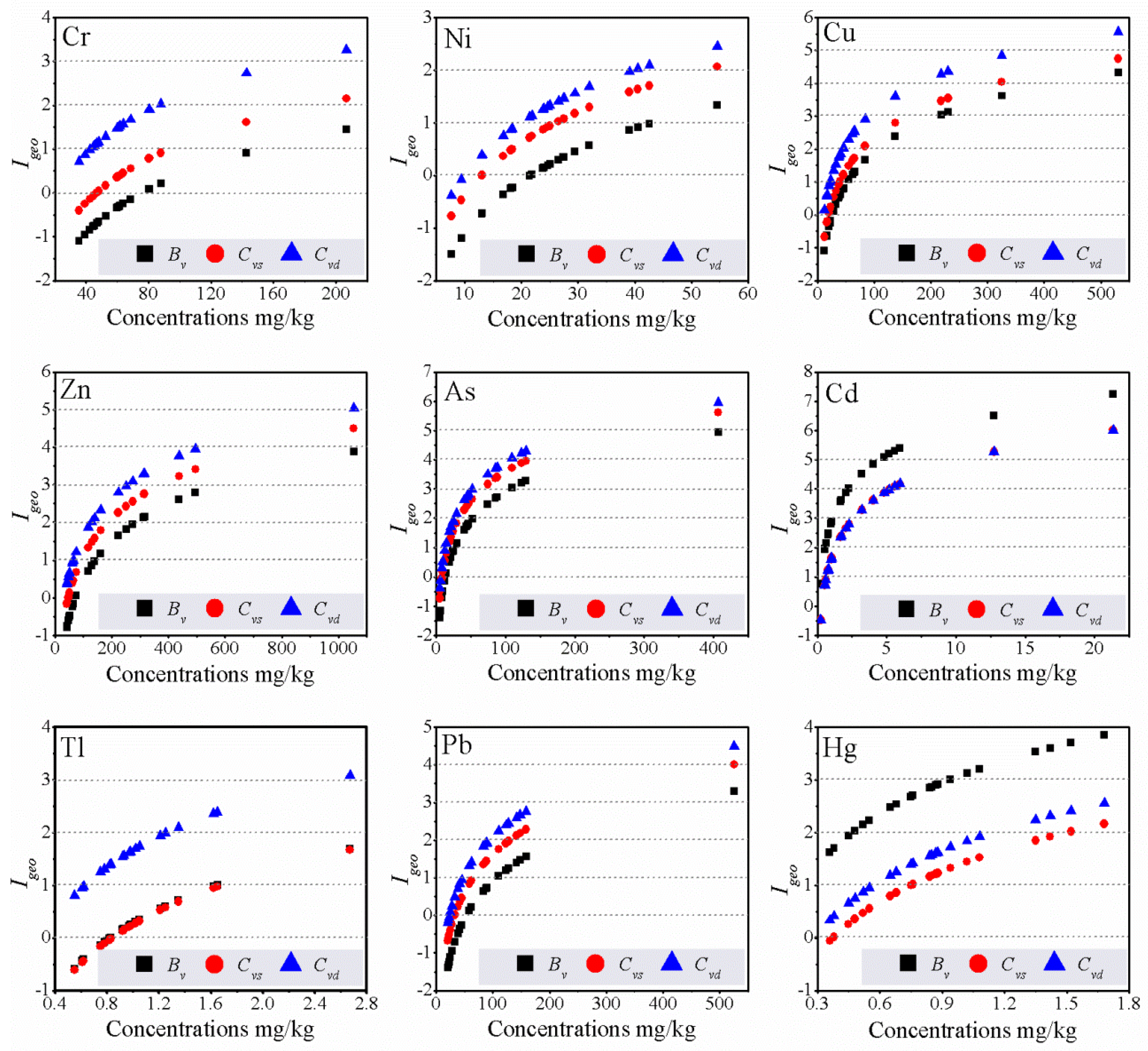
Igeo and EF are risk assessment indexes based on the total concentration and the background value of a single heavy metal, which plays a crucial role in indicating the pollution degree of heavy metal enrichment caused by anthropogenic sources. As shown in Figure 2, it was surprising that the Igeo value of each target heavy metal increased toward its total concentration with a significant decrease was observable toward the background value. Given that the background values of Cr, Ni, Cu, Zn, As, and Pb are in the order of Bv > Cvs > Cvd, the calculated Igeo values showed an opposite decreasing trend. As an example, the range of Igeo values for Cr based on Bv, Cvs and Cvd were −1.09 to 1.45, −0.40 to 2.14, and 0.72–3.27, respectively, and the corresponding evaluation levels also changed significantly, with the highest level showed moderately polluted (Bv) to heavily polluted (Cvd). These results indicate that Igeo values are only related to the total concentration of heavy metals based on selected background values and did not be affected by sediment properties [42]. However, sediment properties and composition can influence the availability of heavy metals in sediments and thus affect the risk assessment [43]. In addition, the risk values of heavy metals with the same content may differ due to the different background values for each type [44]. In contrast, given the EF value is not only affected by total concentrations and background values of heavy metals, also related to the distribution of conservative elements in the matrix. Figure 3 revealed that there was hardly any correlation between EF values of target heavy metals and total heavy metal contents, especially Tl and Hg, indicating that the EF value is susceptible to environmental geological factors [44,45]. This kind of comparison has not been mentioned in previous studies, but it is certain that comparability between these indicators clearly exists.
Traditionally, Igeo and EF values have been compared on the basis of different sampling sites with the purpose of identifying hazardous areas and sources of heavy metals. Figures S2 and S3 visually indicated the differences in Igeo and EF values among sampling sites. In view of the influence of pollution sources and human activities, heavy metal risks invariably fluctuated dynamically, e.g., the Igeo and EF of Cd fluctuated significantly in the whole investigated region, indicating a higher risk at the Maba confluence, especially with an EF value greater than 20 times, which is consistent with our previous findings [2,17]. Given the presence of Bv < Cvs = Cvd, Igeo curves based on the latter two background values were coincident along the path, while EF values were somewhat atypical. In addition, consistent results showed that both the Igeo and EF of a single sample decrease with the increase of background values. These results are expressed in a manner similar to those reported before and are indispensable information for the identification of significant pollution areas and sources in the watershed [10,46].
Synthetically, the selection of background value has significant effect on the enrichment risk of individual sample and individual heavy metal. A more interesting and widely applicable finding is that Igeo values seem to be independent of geological background differences, which can compare the risk of the same heavy metal in different regions, whereas EF values are recommended to be more suitable for comparison of different heavy metals in the same sampling region.
In contrast, PLI, mCd, and RI are indicators to evaluate polymetallic composite pollution based on background values, which can reflect the comprehensive risk of heavy metal enrichment in each sampling area. As shown in Figure 4, although the three indicators are all calculated according to Cf value, their subsequent change trends varied greatly under different background values. PLI showed an increasing trend of Bv < Cvs < Cvd, and mCd followed an order of Cvd > Bv > Cvs, while RI was in the order of Bv > Cvd > Cvs. These differences have rarely been addressed in previous studies [5]. The main reason may be that the three kinds of background values of each heavy metal are always different, and the total concentration of heavy metals at each sampling site also varies significantly, which in turn varies with the heavy metals [31,47]. What counts is that such a great variation in toxicity coefficients inevitably lead to the reverse effect of individual heavy metal risks on the combined risk [6]. Given the difference of total concentrations of Cd reached a maximum of 88.9 times, and the Bv value of Cd was smaller than that of Cvs and Cvd, the mCd and RI values were comparable to or significantly higher than those of the other two. Therefore, it can be inferred that the difference of background value and high risk of a single heavy metal has relatively little influence on PLI, while RI, influenced by the combination of background value and toxicity coefficient, should be closer to the real risk effect.
From the perspective of comprehensive risk assessment in the whole investigated region, the distribution trends observed of PLI, mCd, and RI were basically similar, which was consistent with the results of previous studies [7,48]. The three indicators comprehensively reflected the regional differences in levels of heavy metal pollutants, pollution sources, and metal mobility [49], but there were some subtle differences in the corresponding evaluation levels. The relationship between the distribution of PLI, mCd, RI and the individual heavy metal concentration was further analyzed, and the results are shown in Figures S4–S6. Incredibly, the effects of individual heavy metal concentrations on the comprehensive risk assessment indicators were almost identical. However, the absence of a significant linear correlation between any of the two indicated that the factors influencing these indicators are not unique. This is consistent with the previous results, indicated that the total content does not include information of sediment composition and availability of heavy metals [49], which affects the risk distribution to a certain extent.
In general, the application of PLI, mCd, and RI can reflect the comprehensive risk of heavy metal enrichment in the investigated region and provide similar essential information to indicate the heavily polluted area, but they are not affected by the background value to the same extent. Given the comprehensive consideration of background value and toxicity coefficient, RI seems to be a better choice in the comprehensive risk assessment of heavy metals in sediments.
3.3. Effect of SQG Values on Risk Assessment
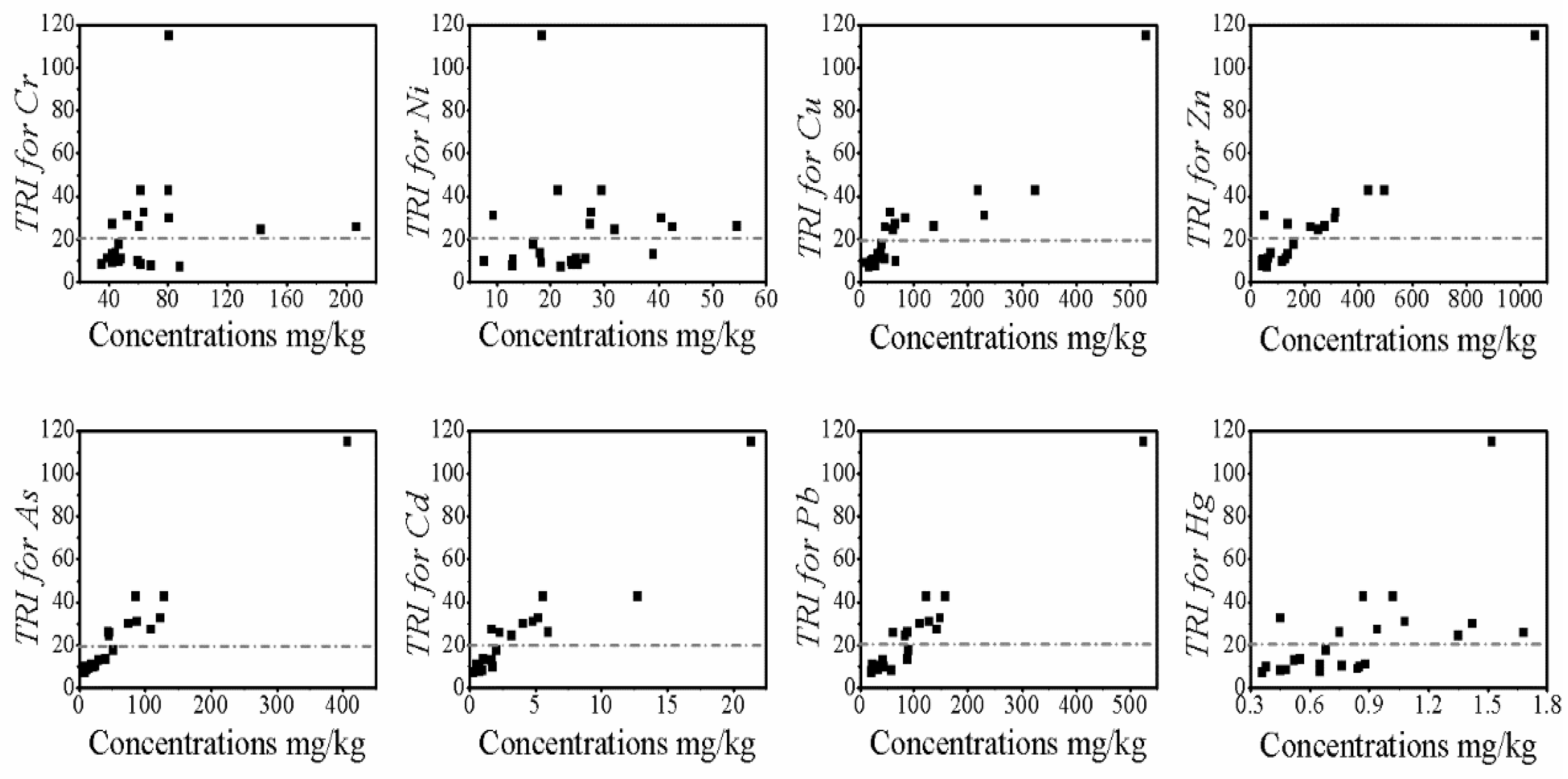
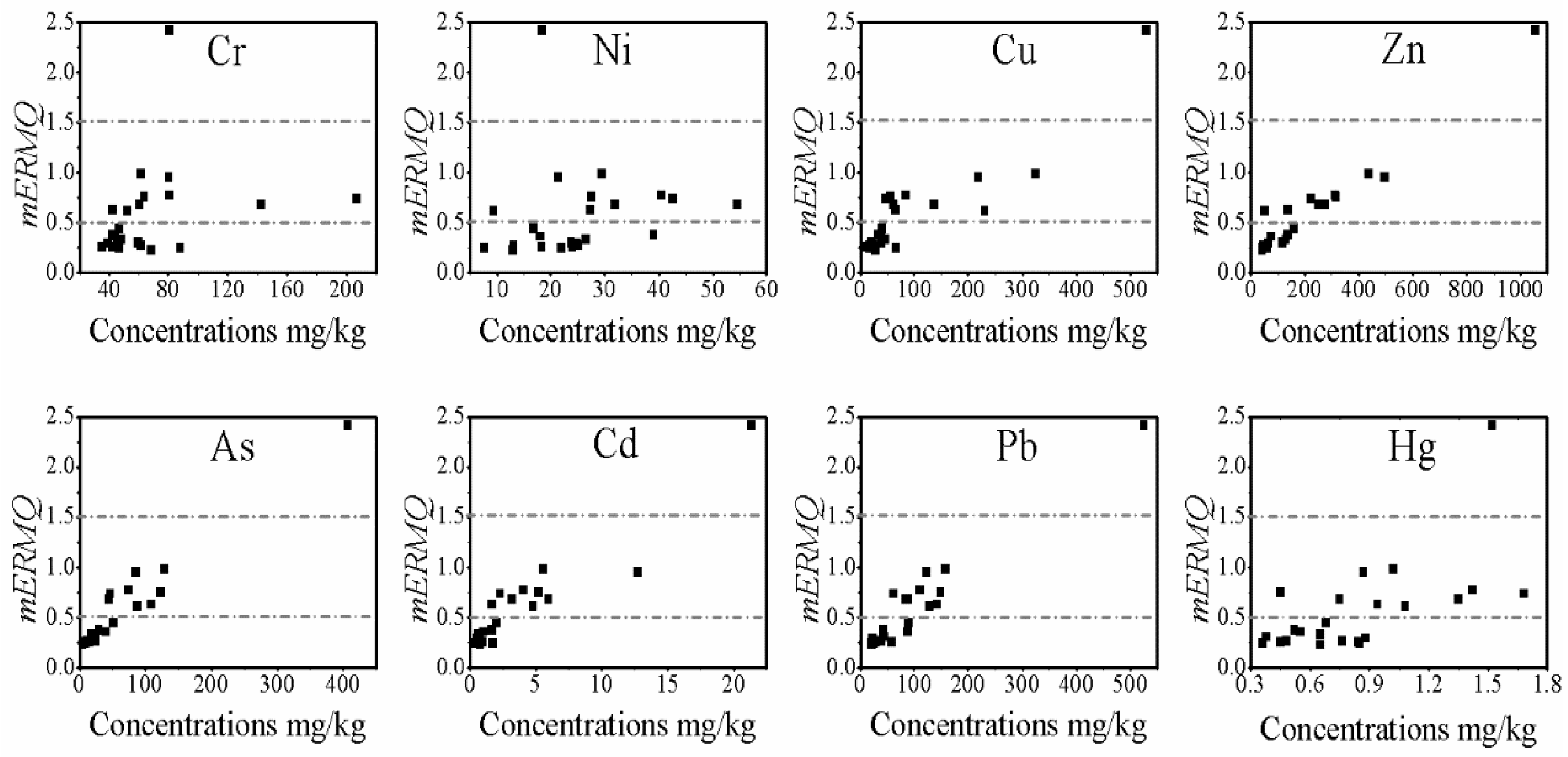
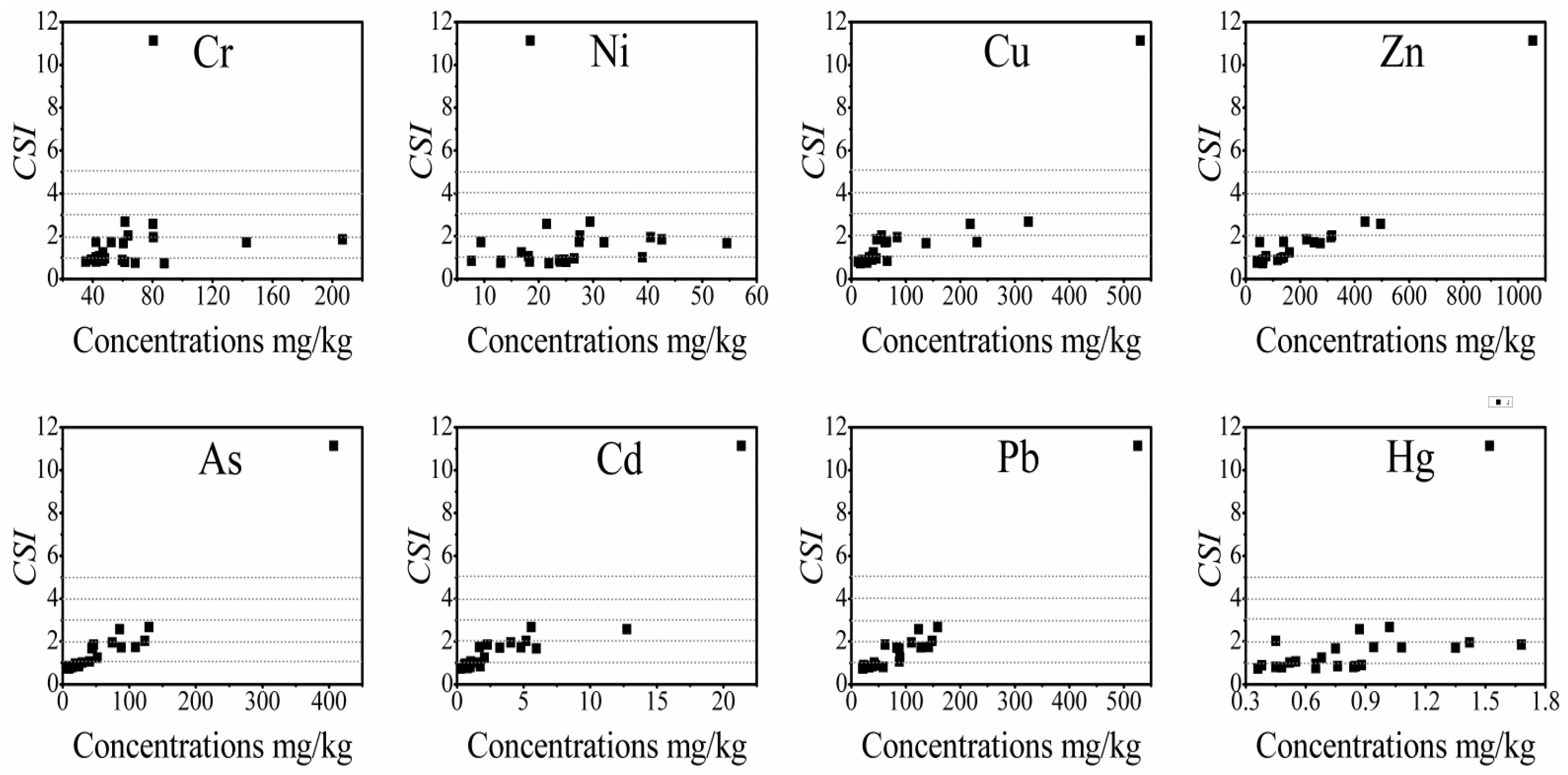
The SQGs are derived from empirically toxic experiments, giving a toxicity indicator for specific aquatic amphipods without considering sediment properties and heavy metal background values [13,27]. TRI, mERMQ, and CSI are comprehensive ecological risk assessment methods of heavy metals in sediments based on SQGs and total contents, which can provide biotoxicity levels of combined heavy metal pollution on aquatic organisms. As shown in Figure 5, Figure 6 and Figure 7, although these three indicators were calculated based on different SQGs [6], the influence of single heavy metal concentration on TRI, mERMQ, and CSI was completely the same as observed from the comprehensive distribution trend. Inevitably, there were subtle differences between the target heavy metals. TRI, mERMQ and CSI were not in conformity with the total contents of Cr, Ni, and Hg, while a significant linear correlation could be observed with the contents of Cu, Zn, As, Cd and Pb. However, the relationship shown does not completely increase in the direction of increasing concentrations. The reason may be that Cu, Zn, As, Cd, and Pb mainly come from anthropogenic sources, such as the discharge of industrial wastewater and domestic sewage, which leads to serious heavy metal pollution with extremely high toxicity to local organisms [2,50]. On the contrary, Cr, Ni, and Hg mainly come from natural sources, and the influence of sediment characteristics cannot be ignored [43,51]. Meanwhile, the results also indicated that the three indicators have similar effects. Regardless of the fact that the results of different indicators for matching objects may be mutually complementary, it seems that choosing one of them is sufficient.
Figure S7 showed the distribution of TRI, mERMQ, and CSI along each sampling site in the whole investigated region, and it could be observed that the trend was almost identical, which further confirms the conclusion as indicated earlier. However, they do not indicate the same level of risk. In this light, TRI indicated that 43.48% of sampling sites had a very high toxicity risk (TRI > 20). mERMQ showed that 4.35% of samples were greater than 1.5 and 39.13% of samples were between 0.5 to 1.5, indicating that 43.48% of samples had a 49% probability of toxicity. Except for the CSI value of one sampling site being as high as 11.14 (ultra-high severity), the other values were all below 3, indicating that 88.86% of sampling areas were below medium-high severity [6,7]. Given the use of different SQGs, although it is impossible to get exactly the same results by applying these three indicators, the evaluation results for the same object are surprisingly consistent.
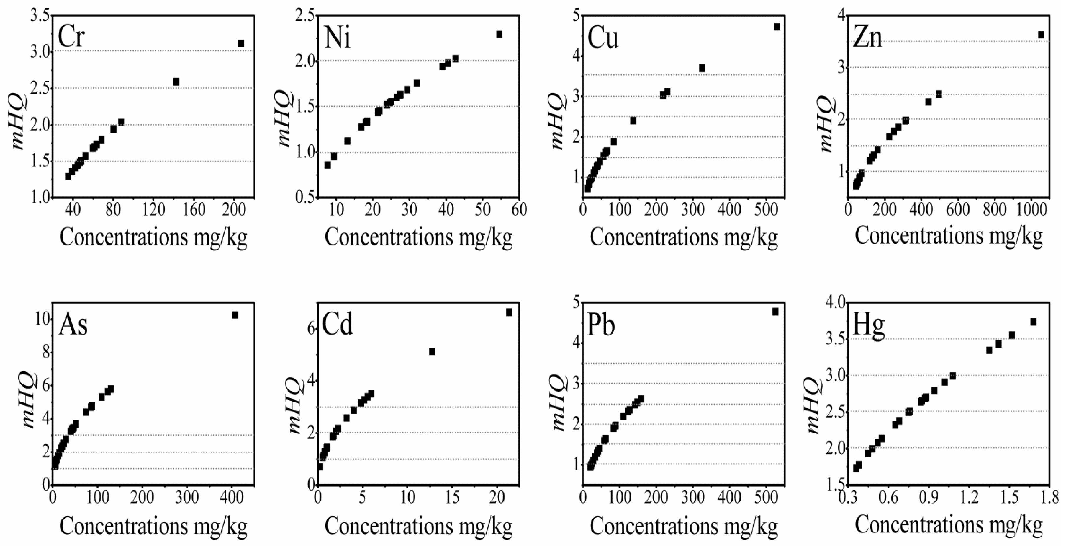
The mHQ assesses levels of contamination by describing each metal concentration observed in sediments with SQGs. The evaluation of mHQ is of utmost importance since it evaluates the risk of individual metal to the biota and the aquatic environment [52]. With respect to the mHQ values obtained, it was completely unexpected that they showed a significant positive linear relationship with individual heavy metal content, and increased towards the increasing of the content of heavy metals (Figure 8), indicating that the mHQ value is only related to the total concentration of heavy metals and has nothing to do with sediment properties [7]. Moreover, Figure 8 also showed the content distribution and corresponding risk of each target heavy metal in the investigated area. Therefore, the corresponding risk can be effectively predicted by measuring the content of heavy metals.
By contrast, it can be obviously observed from Figure S8 that the mHQ distribution of each heavy metal varies with the sampling sites, and it is particularly different from the trend shown by the above comprehensive risk indicators. In this light, no significant anthropogenic pollution sources of Cr, Ni, and Hg were observed, while Cu, Zn, As, Cd, and Pb showed extreme severity of contamination [50]. This firmly confirms that anthropogenic inputs had a key contribution for the enrichment of heavy metals in surface sediments [53,54,55]. Further, more attention should be paid to As, Cd, and Pb at the entrance of the Maba River because of their high contributing ratio to the mHQ values. Undeniably, this representation with the distribution of sampling points is widely adopted, which can be better used to reveal the major pollution sources and the locations of serious pollution in the investigated area.
Synthetically, TRI, mERMQ, and CSI are mainly used for comprehensive ecological risk assessment of composite heavy metal pollution. Although the evaluation degrees of these three indicators are not completely consistent, their effects are basically the same, indicating that any of them can be utilized to meet the requirements rather than all of them. mHQ is used to evaluate the toxicity degree of each heavy metal to aquatic organisms, showing a significant positive linear correlation with the total content of each heavy metal, indicating that this index is not affected by sediment properties and has a wide range of applications.
4. Conclusions
Herein, risk assessment methods of sediment heavy metals calculated based on total content, background values, and SQGs were compared from the perspective of application by substituted of actual monitoring data. The results showed that both Igeo and EF values for the risk assessment of single heavy metal enrichment decreased with the increase of background values. Compared with EF, Igeo also showed a significant positive linear correlation with heavy metal content, indicating that Igeo is not affected by geological factors and is suitable for the comparison of the same heavy metal in different regions. Considering the influence of sediment texture, EF is more suitable for the comparison of different heavy metals in the same sampling interval. PLI, mCd, and RI showed significant differences in response to background values for the comprehensive risk of heavy metal enrichment, and the trends were Bv < Cvs < Cvd, Cvd > Bv > Cvs and Bv > Cvd > Cvs, respectively. Although the evaluation levels of these factors were not identical, their distribution trends were basically the same along with the sampling points, indicating that they have equal evaluation effects. TRI, mERMQ, and CSI showed similar overall distribution trends, but their evaluation levels were not exactly the same, indicating that choosing any one of them can better reflect the toxicity of complex heavy metal pollution to aquatic organisms. Similar to Igeo, mHQ showed a significant positive linear correlation with the content of each heavy metal, indicating that it should not be affected by sediment properties and can be widely used to determine the toxicity of single heavy metals to aquatic organisms. The results of this study have important guiding significance for the selection of evaluation methods for heavy metal pollution in sediments. Further studies regarding the comparison with the method based on speciation content are needed to comprehensively identify the pollution status of heavy metals in sediments.
Supplementary Materials
The following are available online at https://www.mdpi.com/article/10.3390/w14010051/s1, Table S1. Classifications for index of geoaccumulation (Igeo). Table S2. Classifications for enrichment factor (EF). Table S3. Classifications for modified contamination degree (mCd). Table S4. Sediment quality guidelines for metals in freshwater ecosystems that reflect TECs (below which harmful effects are unlikely to be observed) and PECs (above which harmful effects are likely to be observed), and toxicity coefficients (Tri) of heavy metals. Table S5. Classifications for potential ecological risk index (RI). Table S6. Classifications for toxic risk index (TRI). Table S7. Classifications for modified hazard quotient (mHQ). Table S8. Classifications for mean ERM quotient (mERMQ). Table S9. Classifications for contamination severity index (CSI). Table S10. The loading value, eigen value and wi based on principal component analysis and factor analysis. Table S11. Heavy metal concentrations in surface sediments used as control values, all data in mean concentrations, dry weight, mg/kg. Figure S1. Vertical variations of Fe in sediments, all data in mean concentrations, dry weight, mg/kg. The boxes represent 25th and 75th percentiles, the middle horizontal lines represent the 50th percentile, the vertical line ends represent 1th and 99th percentiles, the small squares in the middle represent the mean value, and the diamond black dots represent outliers. Figure S2. The distribution of Igeo values for Cr, Ni, Cu, Zn, As, Cd, Tl, Pb and Hg in the whole investigated region based on different types of background values. Figure S3. The distribution of EF values for Cr, Ni, Cu, Zn, As, Cd, Tl, Pb and Hg in the whole investigated region based on different types of background values. Figure S4. The PLI values of Cr, Ni, Cu, Zn, As, Cd, Tl, Pb and Hg in sediments were calculated based on different types of background values and total concentrations. Figure S5. The mCd values of Cr, Ni, Cu, Zn, As, Cd, Tl, Pb and Hg in sediments were calculated based on different types of background values and total concentrations. Figure S6. The RI values of Cr, Ni, Cu, Zn, As, Cd, Pb and Hg in sediments were calculated based on different types of background values and total concentrations. Figure S7. The distribution of the TRI, mERMQ and CSI values for Cr, Ni, Cu, Zn, As, Cd, Pb and Hg in sediments in the whole investigated region based on different types of SQG values. Figure S8. The distribution of the mHQ values for Cr, Ni, Cu, Zn, As, Cd, Pb and Hg in sediments in the whole investigated region based on different types of SQG values.
Author Contributions
J.L.: Conceptualization, Methodology, Data curation, Roles/Writing—original draft, Writing—review & editing. X.C.: Investigation, Software. H.F.: Roles/Writing—original draft. S.Y.: Roles/Writing—original draft. All authors have read and agreed to the published version of the manuscript.
Funding
This research was funded by the National Natural Science Foundation of China (Grant No. 42007326), the Joint Key Funds of the National and Natural Science Foundation of Guangdong Province, China (Grant No. U1201234), and the Basic and Applied Basic Research Foundation of Guangdong Province (Grant No. 2020A1515110417).
Institutional Review Board Statement
Not applicable.
Informed Consent Statement
Not applicable.
Data Availability Statement
Not applicable.
Conflicts of Interest
The authors declare no conflict of interest.
References
- Cai, L.; Xu, Z.; Qi, J.; Feng, Z.; Xiang, T. Assessment of exposure to heavy metals and health risks among residents near Tonglushan mine in Hubei, China. Chemosphere 2015, 127, 127–135. [Google Scholar] [CrossRef]
- Liao, J.; Chen, J.; Ru, X.; Chen, J.; Wu, H.; Wei, C. Heavy metals in river surface sediments affected with multiple pollution sources, South China: Distribution, enrichment and source apportionment. J. Geochem. Explor. 2017, 176, 9–19. [Google Scholar] [CrossRef]
- Zhai, B.; Zhang, X.; Wang, L.; Zhang, Z.; Zou, L.; Sun, Z.; Jiang, Y. Concentration distribution and assessment of heavy metals in surface sediments in the Zhoushan Islands coastal sea, East China Sea. Mar. Pollut. Bull. 2021, 164, 112096. [Google Scholar] [CrossRef]
- Siddique, M.A.M.; Rahman, M.; Rahman, S.M.A.; Hassan, M.R.; Fardous, Z.; Chowdhury, M.A.Z.; Hossain, M.B. Assessment of heavy metal contamination in the surficial sediments from the lower Meghna River estuary, Noakhali coast, Bangladesh. Int. J. Sediment. Res. 2021, 36, 384–391. [Google Scholar] [CrossRef]
- Yu, G.B.; Liu, Y.; Yu, S.; Wu, S.C.; Leung, A.O.W.; Luo, X.S.; Xu, B.; Li, H.B.; Wong, M.H. Inconsistency and comprehensiveness of risk assessments for heavy metals in urban surface sediments. Chemosphere 2011, 85, 1080–1087. [Google Scholar] [CrossRef]
- Jafarabadi, A.R.; Bakhtiyari, A.R.; Toosi, A.S.; Jadot, C. Spatial distribution, ecological and health risk assessment of heavy metals in marine surface sediments and coastal seawaters of fringing coral reefs of the Persian Gulf, Iran. Chemosphere 2017, 185, 1090–1111. [Google Scholar] [CrossRef]
- Emenike, P.C.; Tenebe, I.T.; Neris, J.B.; Omole, D.O.; Afolayan, O.; Okeke, C.U.; Emenike, I.K. An integrated assessment of land-use change impact, seasonal variation of pollution indices and human health risk of selected toxic elements in sediments of River Atuwara, Nigeria. Environ. Pollut. 2020, 265, 114795. [Google Scholar] [CrossRef]
- Tang, W.; Zhang, W.; Zhao, Y.; Zhang, H.; Shan, B. Basin-scale comprehensive assessment of cadmium pollution, risk, and toxicity in riverine sediments of the Haihe Basin in north China. Ecol. Indic. 2017, 81, 295–301. [Google Scholar] [CrossRef]
- Song, Z.; Song, G.; Tang, W.; Yan, D.; Han, M.; Shan, B. Determining cadmium bioavailability in sediment profiles using diffusive gradients in thin films. J. Environ. Sci.-China 2020, 91, 160–167. [Google Scholar] [CrossRef]
- Islam, M.S.; Ahmed, M.K.; Raknuzzaman, M.; Habibullah-Al-Mamun, M.; Islam, M.K. Heavy metal pollution in surface water and sediment: A preliminary assessment of an urban river in a developing country. Ecol. Indic. 2015, 48, 282–291. [Google Scholar] [CrossRef]
- Xia, P.; Ma, L.; Sun, R.; Yang, Y.; Tang, X.; Yan, D.; Lin, T.; Zhang, Y.; Yi, Y. Evaluation of potential ecological risk, possible sources and controlling factors of heavy metals in surface sediment of Caohai Wetland, China. Sci. Total Environ. 2020, 740, 140231. [Google Scholar] [CrossRef] [PubMed]
- Madzin, Z.; Shai-in, M.F.; Kusin, F.M. Comparing heavy metal mobility in active and abandoned mining sites at Bestari Jaya, Selangor. Procedia Environ. Sci. 2015, 30, 232–237. [Google Scholar] [CrossRef] [Green Version]
- Zhang, Y.; Li, H.; Yin, J.; Zhu, L. Risk assessment for sediment associated heavy metals using sediment quality guidelines modified by sediment properties. Environ. Pollut. 2021, 275, 115844. [Google Scholar] [CrossRef]
- Moreira, L.B.; Bellini Dantas Leite, P.R.; Dias, M.D.L.; Martins, C.D.C.; de Souza Abessa, D.M. Sediment quality assessment as potential tool for the management of tropical estuarine protected areas in SW Atlantic, Brazil. Ecol. Indic. 2019, 101, 238–248. [Google Scholar] [CrossRef]
- Li, R.; Tang, C.; Cao, Y.; Jiang, T.; Chen, J. The distribution and partitioning of trace metals (Pb, Cd, Cu, and Zn) and metalloid (As) in the Beijiang River. Environ. Monit. Assess. 2018, 190, 399. [Google Scholar] [CrossRef]
- Wang, S.; Zhang, C.; Pan, Z.; Sun, D.; Zhou, A.; Xie, S.; Wang, J.; Zou, J. Microplastics in wild freshwater fish of different feeding habits from Beijiang and Pearl River Delta regions, south China. Chemosphere 2020, 258, 127345. [Google Scholar] [CrossRef]
- Liao, J.; Ru, X.; Xie, B.; Zhang, W.; Wu, H.; Wu, C.; Wei, C. Multi-phase distribution and comprehensive ecological risk assessment of heavy metal pollutants in a river affected by acid mine drainage. Ecotoxicol. Environ. Saf. 2017, 141, 75–84. [Google Scholar] [CrossRef]
- Muller, G. Index of geoaccumulation in sediments of the Rhine river. Geojournal 1969, 2, 108–118. [Google Scholar]
- Khan, M.H.R.; Liu, J.; Liu, S.; Li, J.; Cao, L.; Rahman, A. Anthropogenic effect on heavy metal contents in surface sediments of the Bengal Basin river system, Bangladesh. Environ. Sci. Pollut. R. 2020, 27, 19688–19702. [Google Scholar] [CrossRef] [PubMed]
- Sakan, S.M.; Dordevic, D.S.; Manojlovic, D.D.; Predrag, P.S. Assessment of heavy metal pollutants accumulation in the Tisza river sediments. J. Environ. Manag. 2009, 90, 3382–3390. [Google Scholar] [CrossRef]
- Li, Y.; Duanp, Z.; Liu, G.; Kalla, P.; Scheidt, D.; Cai, Y. Evaluation of the Possible Sources and Controlling Factors of Toxic Metals/Metalloids in the Florida Everglades and Their Potential Risk of Exposure. Environ. Sci. Technol. 2015, 49, 9714–9723. [Google Scholar] [CrossRef]
- Birch, G.F.; Olmos, M.A. Sediment-bound heavy metals as indicators of human influence and biological risk in coastal water bodies. ICES J. Mar. Sci. 2008, 65, 1407–1413. [Google Scholar] [CrossRef]
- Hakanson, L. An ecological risk index for aquatic pollution control. A sedi-mentological approach. Water Res. 1980, 14, 975–1001. [Google Scholar] [CrossRef]
- Rajkumar, H.; Naik, P.K.; Rishi, M.S. Evaluation of heavy metal contamination in soil using geochemical indexing approaches and chemometric techniques. Int. J. Environ. Sci. Technol. 2019, 16, 7467–7486. [Google Scholar] [CrossRef]
- Brady, J.P.; Ayoko, G.A.; Martens, W.N.; Goonetilleke, A. Enrichment, distribution and sources of heavy metals in the sediments of Deception Bay, Queensland, Australia. Environ. Mar. Pollut. Bull. 2018, 81, 248–255. [Google Scholar] [CrossRef] [Green Version]
- Zhang, G.; Bai, J.; Zhao, Q.; Lu, Q.; Jia, J.; Wen, X. Heavy metals in wetland soils along a wetland-forming chronosequence in the Yellow River Delta of China: Levels, sources and toxic risks. Ecol. Indic. 2016, 69, 331–339. [Google Scholar] [CrossRef] [Green Version]
- MacDonald, D.D.; Ingersoll, C.G.; Berger, T.A. Development and evaluation of consensus-based sediment quality guidelines for freshwater ecosystems. Environ. Contam. Toxicol. 2020, 39, 20–31. [Google Scholar] [CrossRef] [PubMed]
- Long, E.R.; Ingersoll, C.G.; MacDonald, D.D. Calculation and uses of mean sediment quality guideline quotients: A critical review. Environ. Sci. Technol. 2005, 40, 1726–1736. [Google Scholar] [CrossRef]
- USEPA. Predicting Toxicity to Amphipods from Sediment Chemistry; EPA/600/R–04/030; Office of Emergency and Remedial Response: Washington, DC, USA, 2005.
- Pejman, A.; Bidhendi, G.N.; Ardestani, M.; Saeedi, M.; Baghvand, A. A new index for assessing heavy metals contamination in sediments: A case study. Ecol. Indic. 2015, 58, 365–373. [Google Scholar] [CrossRef]
- Jiao, W.; Ouyang, W.; Hao, F.; Huang, H.; Shan, Y.; Geng, X. Combine the soil water assessment tool (SWAT) with sediment geochemistry to evaluate diffuse heavy metal loadings at watershed scale. J. Hazard. Mater. 2014, 280, 252–259. [Google Scholar] [CrossRef]
- Torres, E.; Ayora, C.; Canovas, C.R.; Garcia-Robledo, E.; Galvan, L.; Sarmiento, A.M. Metal cycling during sediment early diagenesis in a water reservoir affected by acid mine drainage. Sci. Total Environ. 2013, 461, 416–429. [Google Scholar] [CrossRef]
- Zoppini, A.; Ademollo, N.; Amalfitano, S.; Casella, P.; Patrolecco, L.; Polesello, S. Organic priority substances and microbial processes in river sediments subject to contrasting hydrological conditions. Sci. Total Environ. 2014, 484, 74–83. [Google Scholar] [CrossRef]
- Charriau, A.; Lesven, L.; Gao, Y.; Leermakers, M.; Baeyens, W.; Ouddane, B.; Billon, G. Trace metal behaviour in riverine sediments: Role of organic matter and sulfides. Appl. Geochem. 2011, 26, 80–90. [Google Scholar] [CrossRef] [Green Version]
- Fu, J.; Zhao, C.; Luo, Y.; Liu, C.; Kyzas, G.Z.; Luo, Y.; Zhao, D.; An, S.; Zhu, H. Heavy metals in surface sediments of the Jialu River, China: Their relations to environmental factors. J. Hazard. Mater. 2014, 270, 102–109. [Google Scholar] [CrossRef] [PubMed]
- Zhang, R.; Zhou, L.; Zhang, F.; Ding, Y.; Gao, J.; Chen, J.; Yan, H.; Shao, W. Heavy metal pollution and assessment in the tidal flat sediments of Haizhou Bay, China. Mar. Pollut. Bull. 2013, 74, 403–412. [Google Scholar] [CrossRef]
- Deng, Q.; Wei, Y.; Yin, J.; Chen, L.; Peng, C.; Wang, X.; Zhu, K. Ecological risk of human health in sediments in a karstic river basin with high longevity population. Environ. Pollut. 2020, 265, 114418. [Google Scholar] [CrossRef] [PubMed]
- Liao, J.; Wen, Z.; Ru, X.; Chen, J.; Wu, H.; Wei, C. Distribution and migration of heavy metals in soil and crops affected by acid mine drainage: Public health implications in Guangdong Province, China. Ecotoxicol. Environ. Saf. 2016, 124, 460–469. [Google Scholar] [CrossRef] [PubMed]
- Kuriata-Potasznik, A.; Szymczyk, S.; Skwierawski, A.; Glinska-Lewczuk, K.; Cymes, I. Heavy metal contamination in the surface layer of bottom sediments in a flow-through lake: A case study of Lake Symsar in Northern Poland. Water 2016, 8, 358. [Google Scholar] [CrossRef]
- Huu, H.H.; Swennen, R.; Cappuyns, V.; Vassilieva, E.; van Gerven, T.; Tan, V.T. Potential release of selected trace elements (As, Cd, Cu, Mn, Pb and Zn) from sediments in Cam River-mouth (Vietnam) under influence of pH and oxidation. Sci. Total Environ. 2012, 435, 487–498. [Google Scholar]
- Nawrot, N.; Wojciechowska, E.; Pazdro, K.; Szmaglinski, J.; Pempkowiak, J. Uptake, accumulation, and translocation of Zn, Cu, Pb, Cd, Ni, and Cr by P. australis seedlings in an urban dredged sediment mesocosm: Impact of seedling origin and initial trace metal content. Sci. Total Environ. 2021, 768, 144983. [Google Scholar] [CrossRef]
- Zhang, W.; Wu, J.; Zhan, S.; Pan, B.; Cai, Y. Environmental geochemical characteristics and the provenance of sediments in the catchment of lower reach of Yarlung Tsangpo River, southeast Tibetan Plateau. Catena 2021, 200, 105150. [Google Scholar] [CrossRef]
- Liao, J.; Deng, S.; Liu, X.; Lin, H.; Yu, C.; Wei, C. Influence of soil evolution on the heavy metal risk in three kinds of intertidal zone of the Pearl River Estuary. Land Degrad. Dev. 2021, 32, 583–596. [Google Scholar] [CrossRef]
- Diop, C.; Dewaele, D.; Cazier, F.; Diouf, A.; Ouddane, B. Assessment of trace metals contamination level, bioavailability and toxicity in sediments from Dakar coast and Saint Louis estuary in Senegal, West Africa. Chemosphere 2015, 138, 980–987. [Google Scholar] [CrossRef]
- Webster, A.B.; Rossouw, R.; Javier Callealta, F.; Bennett, N.C.; Ganswindt, A. Assessment of trace element concentrations in sediment and vegetation of mesic and arid African savannahs as indicators of ecosystem health. Sci. Total Environ. 2021, 760, 143358. [Google Scholar] [CrossRef]
- Kavehei, A.; Gore, D.B.; Wilson, S.P.; Hosseini, M.; Hose, G.C. Assessment of legacy mine metal contamination using ants as indicators of contamination. Environ. Pollut. 2021, 274, 116537. [Google Scholar] [CrossRef]
- Ma, X.; Zuo, H.; Tian, M.; Zhang, L.; Meng, J.; Zhou, X.; Min, N.; Chang, X.; Liu, Y. Assessment of heavy metals contamination in sediments from three adjacent regions of the Yellow River using metal chemical fractions and multivariate analysis techniques. Chemosphere 2016, 144, 264–272. [Google Scholar] [CrossRef] [PubMed]
- Tunde, O.L.; Oluwagbenga, A.P. Assessment of heavy metals contamination and sediment quality in Ondo coastal marine area, Nigeria. J. Afr. Earth Sci. 2020, 170, 103903. [Google Scholar] [CrossRef]
- Yan, C.; Li, Q.; Zhang, X.; Li, G. Mobility and ecological risk assessment of heavy metals in surface sediments of Xiamen Bay and its adjacent areas, China. Environ. Earth Sci. 2010, 60, 1469–1479. [Google Scholar] [CrossRef]
- Deng, W.; Liu, W.; Li, X.; Yang, Y. Source apportionment of and potential health risks posed by trace elements in agricultural soils: A case study of the Guanzhong Plain, northwest China. Chemosphere 2020, 258, 127317. [Google Scholar] [CrossRef] [PubMed]
- Fdez-Ortiz de Vallejuelo, S.; Gredilla, A.; de Diego, A.; Arana, G.; Manuel Madariaga, J. Methodology to assess the mobility of trace elements between water and contaminated estuarine sediments as a function of the site physico-chemical characteristics. Sci. Total Environ. 2014, 473, 359–371. [Google Scholar] [CrossRef]
- Harikrishnan, N.; Ravisankar, R.; Chandrasekaran, A.; Gandhi, M.S.; Vijayagopal, P.; Mehra, R. Assessment of gamma radiation and associated radiation hazards in coastal sediments of south east coast of Tamilnadu, India with statistical approach. Ecotoxicol. Environ. Saf. 2018, 162, 521–528. [Google Scholar] [CrossRef] [PubMed]
- Duodu, G.O.; Goonetilleke, A.; Ayoko, G.A. Potential bioavailability assessment, source apportionment and ecological risk of heavy metals in the sediment of Brisbane River estuary, Australia. Mar. Pollut. Bull. 2017, 117, 523–531. [Google Scholar] [CrossRef] [PubMed]
- Ustaoglu, F.; Islam, M.S. Potential toxic elements in sediment of some rivers at Giresun, Northeast Turkey: A preliminary assessment for ecotoxicological status and health risk. Ecol. Indic. 2020, 113, 106237. [Google Scholar] [CrossRef]
- Xiao, H.; Shahab, A.; Xi, B.; Chang, Q.; You, S.; Li, J.; Sun, X.; Huang, H.; Li, X. Heavy metal pollution, ecological risk, spatial distribution, and source identification in sediments of the Lijiang River, China. Environ. Pollut. 2021, 269, 116189. [Google Scholar] [CrossRef]
Figure 1.
Vertical variations of heavy metals in sediments, all data in mean concentrations, dry weight, mg/kg. The boxes represent 25th and 75th percentiles, the middle horizontal lines represent the 50th percentile, the vertical line ends represent 1st and 99th percentiles, the small squares in the middle represent the mean value, and the diamond black dots represent outliers.

Figure 2.
The Igeo values of Cr, Ni, Cu, Zn, As, Cd, Tl, Pb, and Hg in sediments were calculated based on different types of background values and total concentrations.
Figure 2.
The Igeo values of Cr, Ni, Cu, Zn, As, Cd, Tl, Pb, and Hg in sediments were calculated based on different types of background values and total concentrations.

Figure 3.
The EF values of Cr, Ni, Cu, Zn, As, Cd, Tl, Pb, and Hg in sediments were calculated based on different types of background values and total concentrations.
Figure 3.
The EF values of Cr, Ni, Cu, Zn, As, Cd, Tl, Pb, and Hg in sediments were calculated based on different types of background values and total concentrations.

Figure 4.
The distribution of the PLI, mCd, RI values for Cr, Ni, Cu, Zn, As, Cd, Tl, Pb, and Hg in sediments in the whole investigated region based on different types of background values.
Figure 4.
The distribution of the PLI, mCd, RI values for Cr, Ni, Cu, Zn, As, Cd, Tl, Pb, and Hg in sediments in the whole investigated region based on different types of background values.

Figure 5.
The TRI values of Cr, Ni, Cu, Zn, As, Cd, Pb, and Hg in sediments based on SQG values (TEL, PEL) and total heavy metal concentrations.
Figure 5.
The TRI values of Cr, Ni, Cu, Zn, As, Cd, Pb, and Hg in sediments based on SQG values (TEL, PEL) and total heavy metal concentrations.

Figure 6.
The mERMQ values of Cr, Ni, Cu, Zn, As, Cd, Pb and Hg in sediments based on SQG values (ERM) and total heavy metal concentrations.
Figure 6.
The mERMQ values of Cr, Ni, Cu, Zn, As, Cd, Pb and Hg in sediments based on SQG values (ERM) and total heavy metal concentrations.

Figure 7.
The CSI values of Cr, Ni, Cu, Zn, As, Cd, Pb, and Hg in sediments based on SQG values (ERL, ERM) and total heavy metal concentrations.
Figure 7.
The CSI values of Cr, Ni, Cu, Zn, As, Cd, Pb, and Hg in sediments based on SQG values (ERL, ERM) and total heavy metal concentrations.

Figure 8.
The mHQ values of Cr, Ni, Cu, Zn, As, Cd, Pb, and Hg in sediments based on SQG values (TEL, PEL, SEL) and total heavy metal concentrations.
Figure 8.
The mHQ values of Cr, Ni, Cu, Zn, As, Cd, Pb, and Hg in sediments based on SQG values (TEL, PEL, SEL) and total heavy metal concentrations.


Table 1.
Comparison of three types of background values of heavy metals and Fe in sediments, including soil background value (Bv), control value of surface sediment (Cvs), and control value of deep sediment (Cvd) in Guangdong Province, dry weight, mg/kg.
Table 1.
Comparison of three types of background values of heavy metals and Fe in sediments, including soil background value (Bv), control value of surface sediment (Cvs), and control value of deep sediment (Cvd) in Guangdong Province, dry weight, mg/kg.
| Metals | Cr | Ni | Cu | Zn | As | Cd | Tl | Pb | Hg | Fe |
|---|---|---|---|---|---|---|---|---|---|---|
| Bv | 50.53 | 14.4 | 17.65 | 47.71 | 8.9 | 0.094 | 0.55 | 35.78 | 0.078 | 26,400 |
| Cvs | 31.16 | 8.7 | 13.22 | 31.15 | 5.56 | 0.22 | 0.56 | 21.79 | 0.25 | 33,846 |
| Cvd | 14.31 | 6.64 | 7.49 | 21.44 | 4.39 | 0.22 | 0.21 | 15.58 | 0.19 | 31,065 |
Publisher’s Note: MDPI stays neutral with regard to jurisdictional claims in published maps and institutional affiliations. |
© 2021 by the authors. Licensee MDPI, Basel, Switzerland. This article is an open access article distributed under the terms and conditions of the Creative Commons Attribution (CC BY) license (https://creativecommons.org/licenses/by/4.0/).
Share and Cite
MDPI and ACS Style
Liao, J.; Cui, X.; Feng, H.; Yan, S. Environmental Background Values and Ecological Risk Assessment of Heavy Metals in Watershed Sediments: A Comparison of Assessment Methods. Water 2022, 14, 51. https://doi.org/10.3390/w14010051
AMA Style
Liao J, Cui X, Feng H, Yan S. Environmental Background Values and Ecological Risk Assessment of Heavy Metals in Watershed Sediments: A Comparison of Assessment Methods. Water. 2022; 14(1):51. https://doi.org/10.3390/w14010051
Chicago/Turabian StyleLiao, Jianbo, Xinyue Cui, Hai Feng, and Shangkun Yan. 2022. "Environmental Background Values and Ecological Risk Assessment of Heavy Metals in Watershed Sediments: A Comparison of Assessment Methods" Water 14, no. 1: 51. https://doi.org/10.3390/w14010051
Note that from the first issue of 2016, this journal uses article numbers instead of page numbers. See further details here.