
Development and Assessment of Water-Level Prediction Models for Small Reservoirs Using a Deep Learning Algorithm


Department of Environmental Management, Faculty of Agriculture, Kindai University, 3327-204 Nakamachi, Nara 631-8505, Japan
*
Authors to whom correspondence should be addressed.
Water 2022, 14(1), 55; https://doi.org/10.3390/w14010055
Submission received: 29 November 2021
/
Revised: 22 December 2021
/
Accepted: 23 December 2021
/
Published: 28 December 2021
(This article belongs to the Section Urban Water Management)
Abstract
:In this study, we aimed to develop and assess a hydrological model using a deep learning algorithm for improved water management. Single-output long short-term memory (LSTM SO) and encoder-decoder long short-term memory (LSTM ED) models were developed, and their performances were compared using different input variables. We used water-level and rainfall data from 2018 to 2020 in the Takayama Reservoir (Nara Prefecture, Japan) to train, test, and assess both models. The root-mean-squared error and Nash–Sutcliffe efficiency were estimated to compare the model performances. The results showed that the LSTM ED model had better accuracy. Analysis of water levels and water-level changes presented better results than the analysis of water levels. However, the accuracy of the model was significantly lower when predicting water levels outside the range of the training datasets. Within this range, the developed model could be used for water management to reduce the risk of downstream flooding, while ensuring sufficient water storage for irrigation, because of its ability to determine an appropriate amount of water for release from the reservoir before rainfall events.
1. Introduction
Over 150,000 small-to-medium-sized irrigation reservoirs exist in Japan. Many of them are small, ranging from several hundred to 100,000 m cubed. Approximately 70% of them were built before modern times, or over 150 years ago, for irrigation purposes, and the oldest recorded pond was built over 1500 years ago. Many of the irrigation reservoirs have deteriorated, and the number of suitable reservoirs is continuously decreasing. In recent years, natural disasters such as torrential rains and earthquakes have resulted in floods and the collapse of dikes in several reservoirs. Reservoir floods and collapses induced by such disasters have led to increased secondary disasters in downstream areas. Thus, there has been growing interest in monitoring the hydrological parameters of reservoirs and predicting the risk of flooding using modern sensing and simulation technologies [1,2].
Increasing studies have focused on the development and application of prediction models for large dams or major rivers, considering the size of the associated areas of interest. However, small reservoirs are of relatively low interest for administrators and researchers when considering the lack of available data and the relatively low number of beneficiaries. Recent developments in modeling techniques and low-cost information and communication technologies have enabled the development of hydrological models for small reservoirs.
Models for water-level predictions are based on two approaches, namely, conceptual models and physical and data-driven models [3]. The conceptual or physical-based models utilize hydrological variables such as evaporation, infiltration rate, and soil moisture content in the model architectures. The data-driven models identify relationships between precipitation and water level directly from the obtained hydrological data [4].
Currently, machine learning is often used as a data-driven model in hydrology. For instance, data-driven models have been used to assess groundwater quality [5,6,7] and to predict drought [8,9,10,11] and evapotranspiration [12,13,14]. Hydrological models using artificial neural networks have seen vigorous increases in machine learning [6,9,10,11,12,13,14].
The artificial neural network (ANN) technique is a typical data-driven or black-box-type method that has received attention for applications in hydrological modeling owing to its ability to reproduce nonlinear processes with relatively few requirements for physical input variables. The recent development of graphical processor units has accelerated the development of deep learning applications. Deep learning allows computational models that are composed of multiple processing layers to learn representations of data with multiple levels of abstraction [15].
A recurrent neural network (RNN) is a type of ANN that includes a recurrent layer. The difference between a recurrent layer and a regular fully connected hidden layer is that neurons within a recurrent layer can be connected to each other [16]. However, a limitation of RNN applications is their inability to learn and process “long-term dependency” tasks automatically, resulting in a decline in prediction accuracy. Long short-term memory (LSTM) networks [17] solved this problem by having a longer short-term memory life over the input, thereby paving the way for more efficient and intensive training with time-series datasets. A lower error rate was found with an LSTM network than with a simple RNN and gated recurrent units (GRUs) [18], which employ simpler long-short dependences than LSTM networks during natural language processing [19].
A commonly used LSTM network is the multi-input, single-output type. The explanatory variables are entered in the input layer via the LSTM unit as time-series data for serial processing. The single output layer produces a single output for explanatory variables. This is the most common and simplest structure for LSTM networks and is variably called the single-output model, the sequence-to-vector model, or the many-to-one model. This model is often used for document-to-genre classification [20,21], tagging [22], and other applications for natural language-processing tasks.
The encoder–decoder or sequence-to-sequence model is a multi-input, multi-output structured model that is built by combining each input layer and output layer. Using this model, the series data for each time step are first entered into the input layer. Thereafter, unlike the simple LSTM model, only the weighting of the intermediate layer is transmitted to the output LSTM unit. Subsequently, the output LSTM unit acquires the internal weighting from the input layer for the output layer. The output layer, in turn, uses the results obtained from the first step as the input for the next time step. By repeating this sequence, a continuous output is made possible using the LSTM unit [23]. This type of mechanism is suitable for handling natural language tasks, machine translation, and speech recognition [24].
Considering the advantage of time-series analysis, the LSTM applications have been increasing in the fields of hydrology and water-resource engineering [25]. As an example, Hu et al. [26] developed hydrological models using ANN and LSTM algorithms, and studies have compared LSTM with other hydrological models for stream-flow analysis [27,28,29]. The results of these studies demonstrate the superiority of predictions made using LSTM models. In addition, the efficiency of LSTM analysis has been shown in a runoff simulation model during snowfalls [30] and management models for reservoir operations [31,32]. Development in this field also includes “hybrid models” that combine physical theories in hydrology with the LSTM algorithm [14,32] and models that combine several deep learning algorithms [33,34] or statistical techniques [27,35].
A recent application of LSTM was reported by Li et al. [36], which focused on the input/output structures of the LSTM. Furthermore, an LSTM encoder–decoder (LSTM ED) approach was recently applied for runoff analysis [37,38]. Compared to the conventional single-output LSTM (LSTM SO) model, these models are expected to reduce errors even with relatively long steps with higher stability [37]. In addition, a few LSTM ED applications have been developed in various fields, although these models require verification [37]. Therefore, in this study, we attempted to construct a simple and practical water-level prediction model using the LSTM ED model for small-to-medium-sized agricultural reservoirs where observations are limited.
We aimed to develop and assess hydrological models using the deep learning algorithm, LSTM ED, for predicting water levels applicable to agricultural reservoirs. An LSTM SO model was also developed, and its performance was compared with that of the LSTM ED model. Thereafter, using the LSTM ED model, we examined outputs from different learning and testing periods with different hydrological data periods. The water level, rainfall data, and discharge events from 2018 to 2020 in the Takayama Reservoir (Nara Prefecture, Japan) were used in our analysis.
2. Materials and Methods
2.1. Data Collection
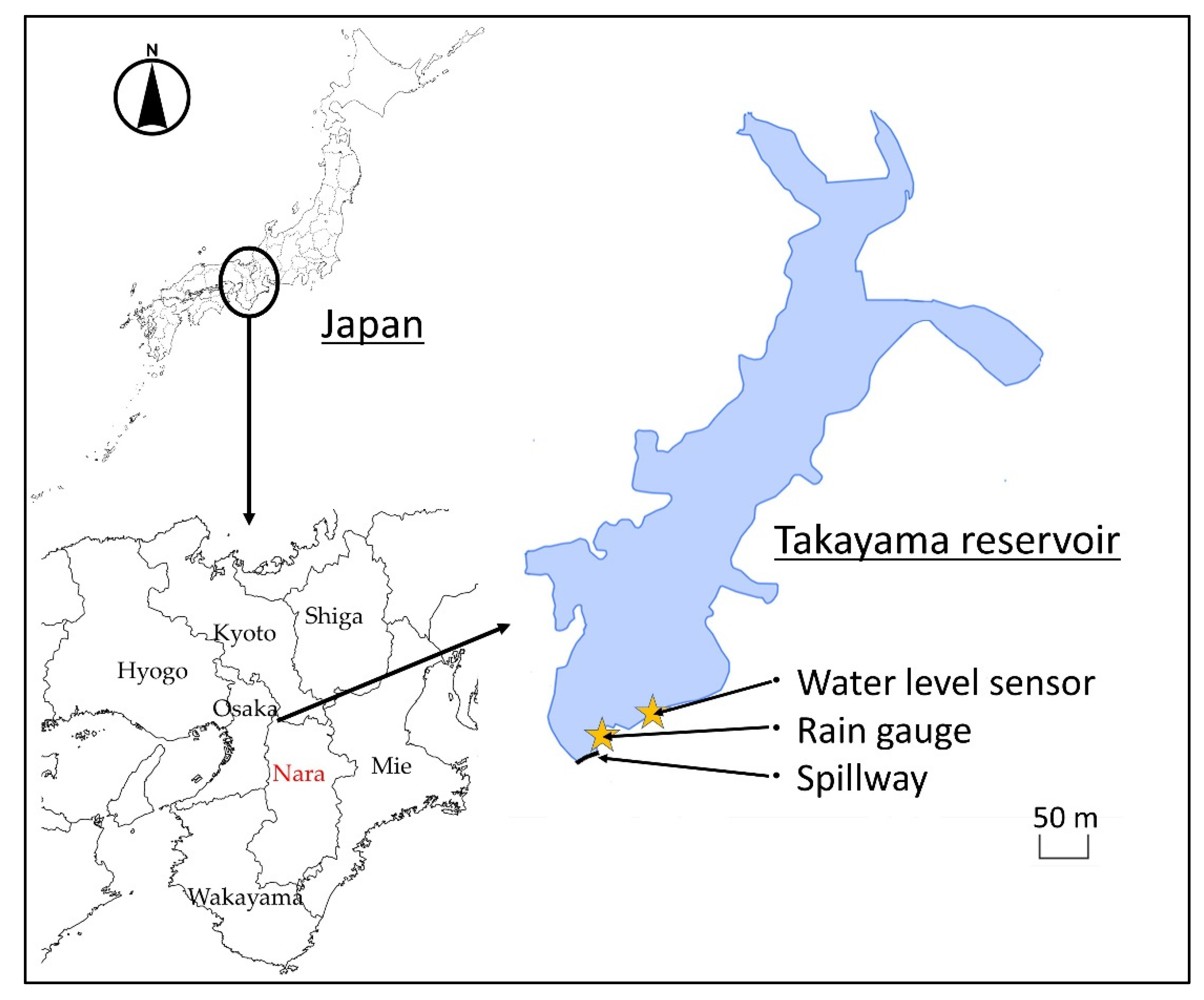
To develop the model, data were obtained from the Takayama Reservoir, located in Takayama Town, Ikoma City, Nara Prefecture, Japan (Figure 1). The outflow from the Takayama Reservoir joins the Tomio River, which is a tributary of the Yamato River Basin. The specifications of the Takayama Reservoir are presented in Table 1. The Takayama Reservoir is one of the largest agricultural reservoirs among approximately 4000 reservoirs in Nara Prefecture. It was constructed in 1956 by the prefectural government and managed by Kitayamato Land Improvement District, which is a water-user association with a membership of approximately 900 farm households. Reservoir water is used for paddy rice cultivation and is normally distributed from May (during the land-preparation period) to September, which is approximately 2 weeks before harvesting. All drainage water from the paddy flows into the Tomio River, mostly through a downstream residential area. Therefore, the Takayama Reservoir plays a hydrologically important role in preventing flooding in the downstream area.
A water-level sensor and a rain gauge were installed at the periphery of the reservoir (Figure 1) to monitor hourly water levels and precipitation. Information regarding water discharge from the reservoir was provided by the Kita Yamato Land Improvement District. These data were collected from 1 July 2018 to 24 July 2020.
2.2. LSTM Model Development
LSTM cells can be described with the following equations:
where, it is the input gate, ft is the forget gate, ct is the cell state at time step (t), ot is the forget gate, ht is the output, σ is the sigmoid function, W is the weight of the respective (x) neurons, b is the bias, and i is the input gate. Long-term memory is made possible by adding (i) the long-term ct−1 and (ii) the short-term feature value ht−1, to i.
The LSTM SO model can be described with the following equation:
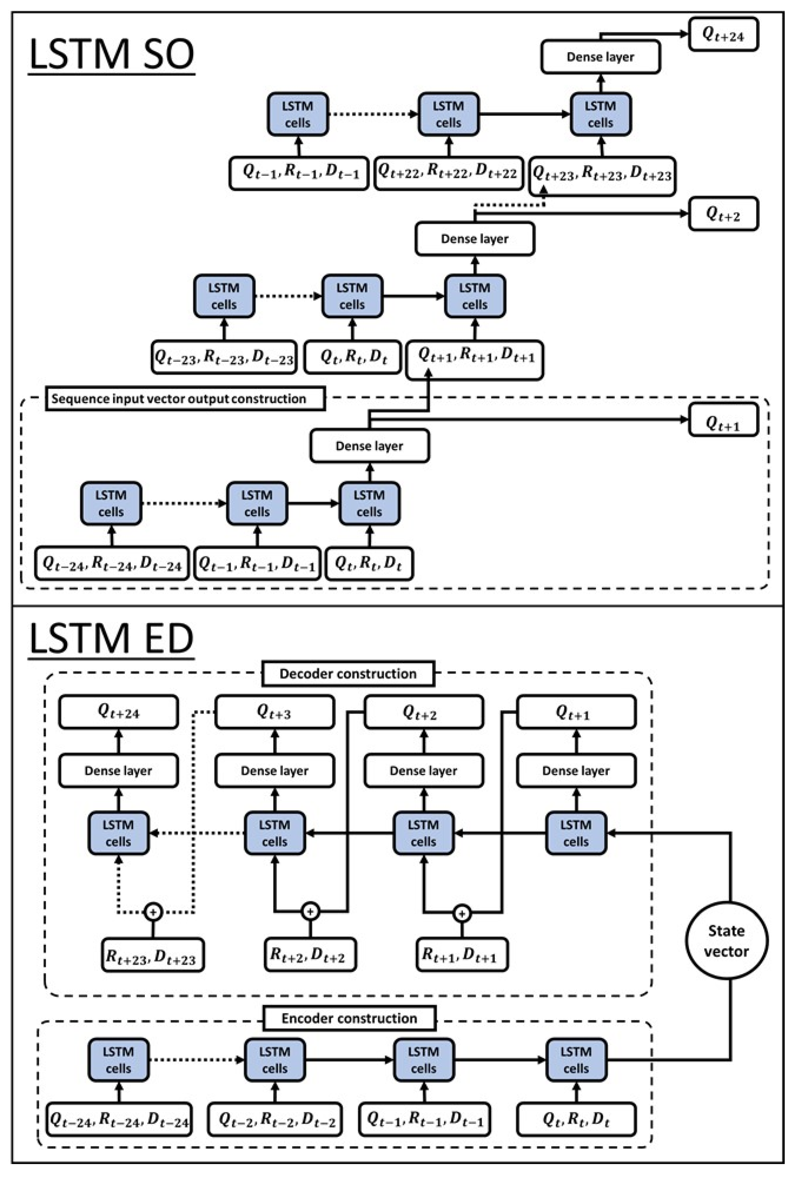
where, is the predicted water level after 1 h. The right side of the equation indicates LSTM cells that perform the single output, and , , and indicate the observed water level, precipitation, and discharge from time t−24 to t, respectively. The calculation was repeated 24 times to make continuous predictions for up to 24 h. The left diagram in Figure 2 shows the structure of the LSTM SO model. As shown in Figure 2, past rainfall and water-level changes were inserted in the input layer, and the predicted water level at the time following the time of the last input value was inserted in the output layer. With this basic structure, the output obtained was used as the next input. By repeating this, the prediction was performed for up to 24 h.
Similarly, the LSTM ED model can be expressed with the following equation:
where, is the predicted water level from t + 1 to t + 24, and , , and indicate the predicted water level, precipitation, and discharge from t + 1 to t + 23, respectively. The right side of the equation indicates the LSTM cells performing the decoder function. S indicates the feature value (state vector) extracted from past information and can be expressed as:
The right side of Equation (8) describes the mathematical relationship when LSTM cells function as the encoder. The bottom diagram in Figure 2 shows the structure of the LSTM ED model. , , and are the observed water level, precipitation, and discharge from time t−24 to time t, respectively. With the LSTM ED model, the rainfall and water-level data for the past 24 h are entered into the encoder for each hour. The state vector extracted from the input layer is entered into the decoder. The first LSTM cells generate the weighting of the intermediate layer and return the output value as the input value for the next time step. This process is repeated for up to 24 h to make predictions. In addition, the predicted rainfall and discharge events are entered in the decoder as input variables.
The difference between the two models is that, for the LSTM ED model, the output is linked to the middle layers, whereas the LSTM SO model does not have such a linkage. A model that predicts the water level 1 h later using the observed data for current and past timepoints functions as a single unit, and continuous prediction is possible by inputting the predicted value to the next unit.
2.3. LSTM Model Assessment
We examined the LSTM SO and LSTM ED models with different input and output variables, as shown in Table 2.
In many cases, the catchment area and the relationship between the storage capacity and water levels are not acquired for small reservoirs. Without this information, it is not possible to accurately estimate the relationship between the water level and inflow to the reservoir. Furthermore, from a management perspective, it is desirable, as much as possible, to predict the water level directly from simple observation data. Therefore, we attempted to predict the water level from simple input variables, such as the changes in the water level, rainfall intensity at a single observation point, and the occurrence of a discharge event. Water level fluctuates considerably throughout the year; thus, if the water level is simply used as an output, then it may show negligible changes in the water level due to rainfall. Therefore, the amount of change in the water level was used as the input variable. However, in this case, the relationship between the inflow amount and the water level may not be reflected well because of the influence of the geometry of the reservoir, which is normally a reverse cone shape. Therefore, we considered solving both problems by factoring in both water level and changes in the water as input variables, and water-level changes as an output variable.
To this end, we prepared the LSTM SO1 and ED1 models that used both water level and water-level change as input variables. In addition, the LSTM SO2 and ED2 models were constructed, which used only the water level as both input and output variables, whereas the LSTM SO2 and ED3 models used only the water-level change as an input variable for comparison purposes.
Table 3 shows the input parameters used in the models. The same parameters were used for all models except for epochs. Epochs indicated the number of cycles through the training dataset and were set to different values because they were determined using the early stopping method to avoid overfitting. Validation, conducted by attempting 1 to 24 h input lags, revealed there was no effect on the accuracy, even after 15 h. Therefore, the input length for the LSTM ED model and the LSTM SO model was set to 24 h, as small-scale reservoirs have short time lags in rainfall runoff. The output length for the LSTM ED models was set to 24 h, and that for the LSTM SO models was set to 1 h, and this length was repeated for up to 24 h. The hidden unit, which indicates the number of LSTM cells, was set to 20. The batch size (i.e., the number of batches parallelized during batch processing in order to perform parallel processing and increase the training efficiently) was validated with 1 to 512; it was set to 64, because it presented the best performance among them. The Adam optimizer [39], which is based on the stochastic gradient-descent method, was used as the optimization function. The Adam is computationally efficient and is also appropriate for non-stationary objectives and problems with very noisy and/or sparse gradients [39]. The loss function employed the mean squared error, which is generally used for loss functions.
2.4. Ensemble Learning Method
In this study, we used the ensemble learning method. An ensemble consists of a set of individually trained models whose outputs are combined when predicting novel instances [40]. In deep learning, each neuron is weighted during learning, and the differences in the initial weighting value affect the weighting after the final learning step. Ensemble learning using different initial weightings is a simple and effective method for neural networks [40]. We used the ensemble-learning method in such a way that the initial weighting was randomly determined to construct 20 individually trained post-learning models.
2.5. Comparing the Performances of Different Models
The root-mean-squared error (RMSE) was used to evaluate the models. The RMSE can be used to estimate the absolute error between the predicted and measured values and can be expressed as follows:
where, Yobs and Ypre are the observed and predicted water-level changes at time step i, respectively, and N is the total number of time steps.
The Nash–Sutcliffe efficiency (NSE) is an index that evaluates models for estimating the size of variation. Its range is −∞ to 1, and values closer to 1 reflect greater accuracy. If the NSE index is 0.7, then the reproducibility of the model is considered high. The NSE is expressed using the following equation:
where, Yave is the average water level observed at all time points.
In this study, we first compared the LSTM ED and LSTM SO models with different input and output variables using the above two evaluation equations and clarified how the structural differences affected the predictions. Next, the water-level input methods were compared using the LSTM ED1, LSTM ED2, and LSTM ED3 models, assuming that the water level was predicted in a situation where there was a record of the spill event, but there was no quantitative spill data. The performance of the models when using water-level changes and water levels as input variables was also compared.
To confirm that a given model could reproduce the relationship between the water level and reservoir capacity, an analysis was performed to simulate water-level changes after a rainfall event with different initial water levels.
The above analyses were conducted to evaluate the comparative advantages of the LSTM ED models and assess the performance of the developed model with minimal hydrological information.
3. Results and Discussion
3.1. Field Data
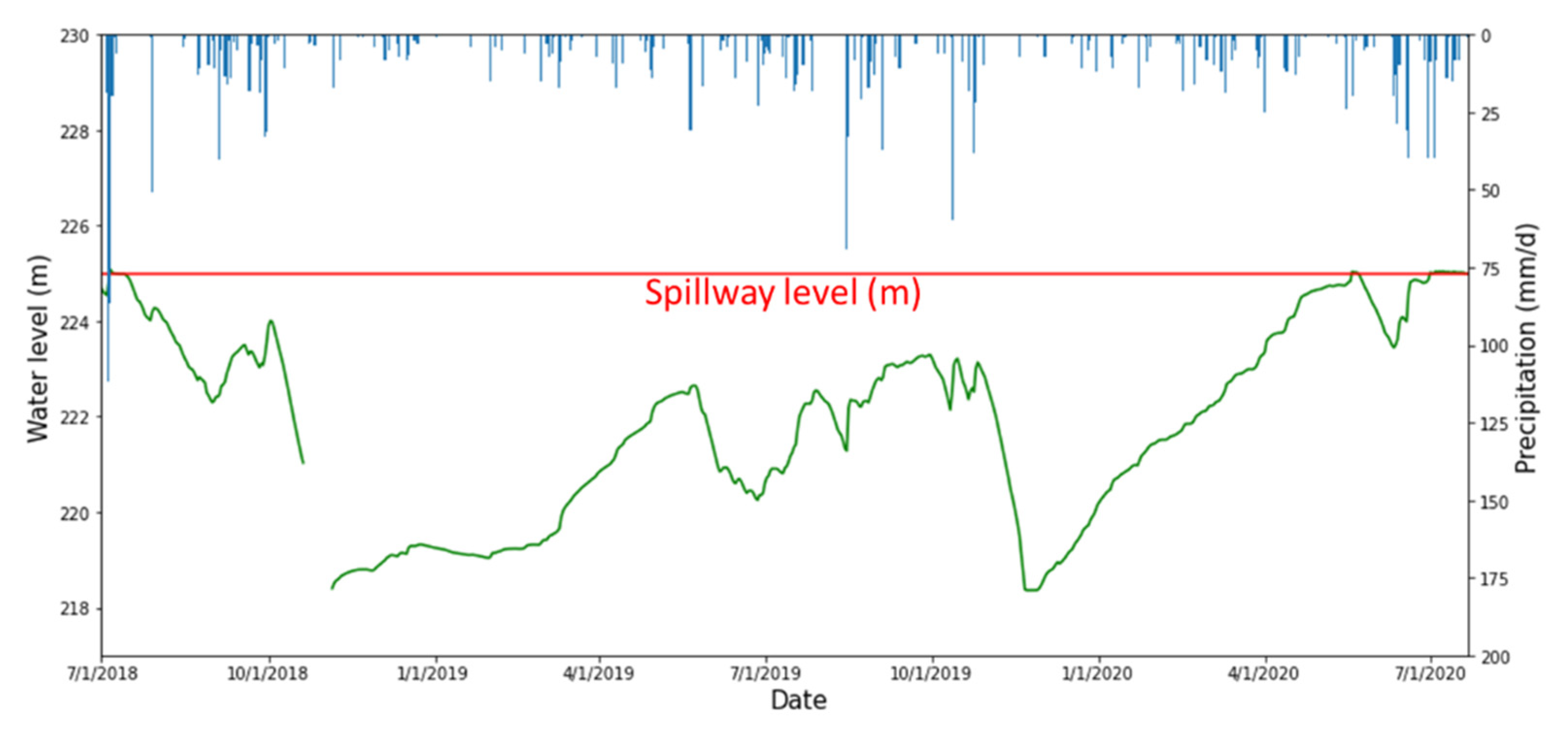
An overview of the data obtained in this study is presented in Figure 3. The maximum water level was equal to the height of the spillway, which is 225 m above sea level. Spill water was observed in both 2018 and 2020. The water-level data could not be obtained from 20 October to 5 November 2018, because of a problem with the data-transmission device. Table 4 summarizes the data obtained during the study.
3.2. Comparison of the LSTM Models
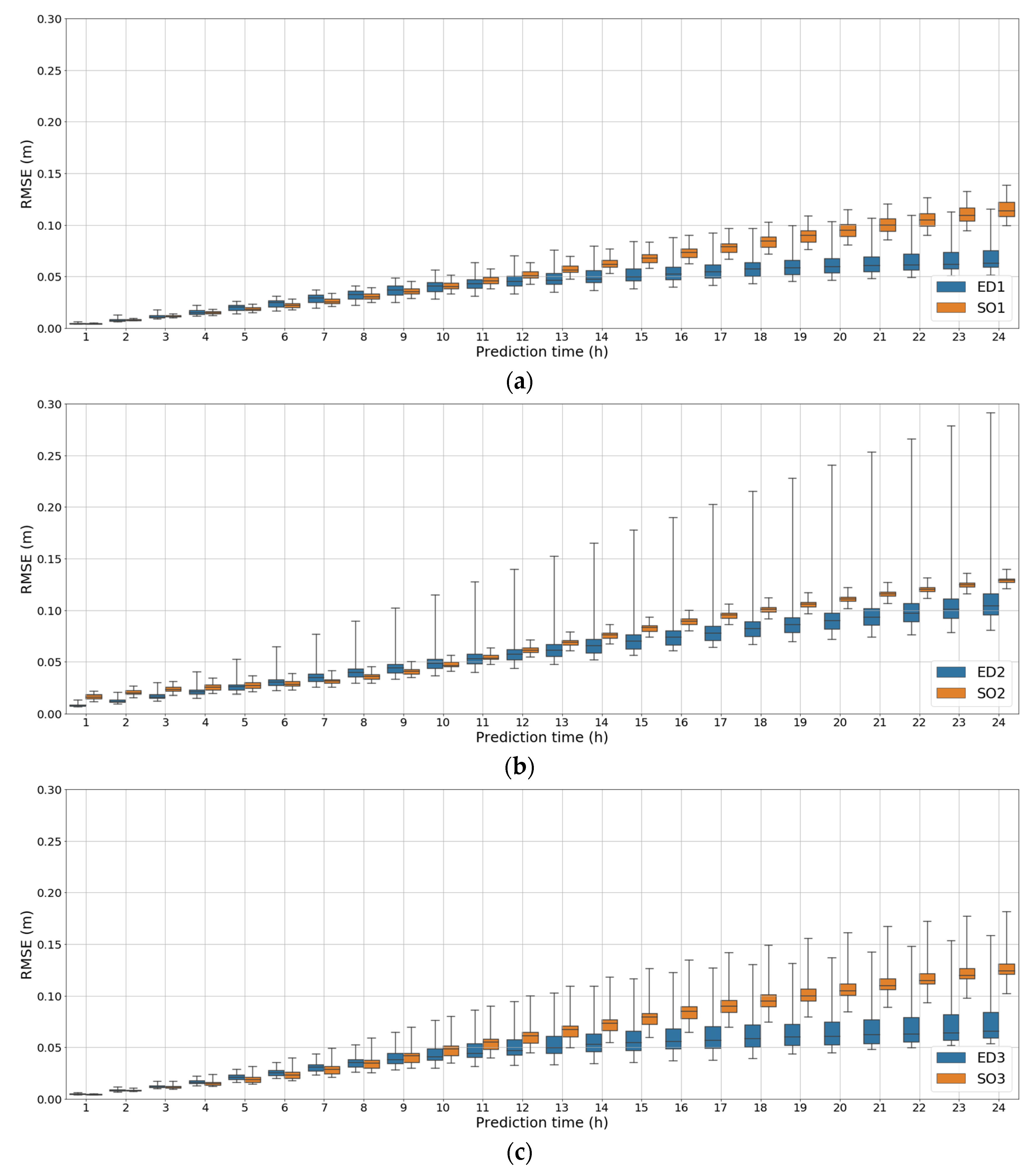
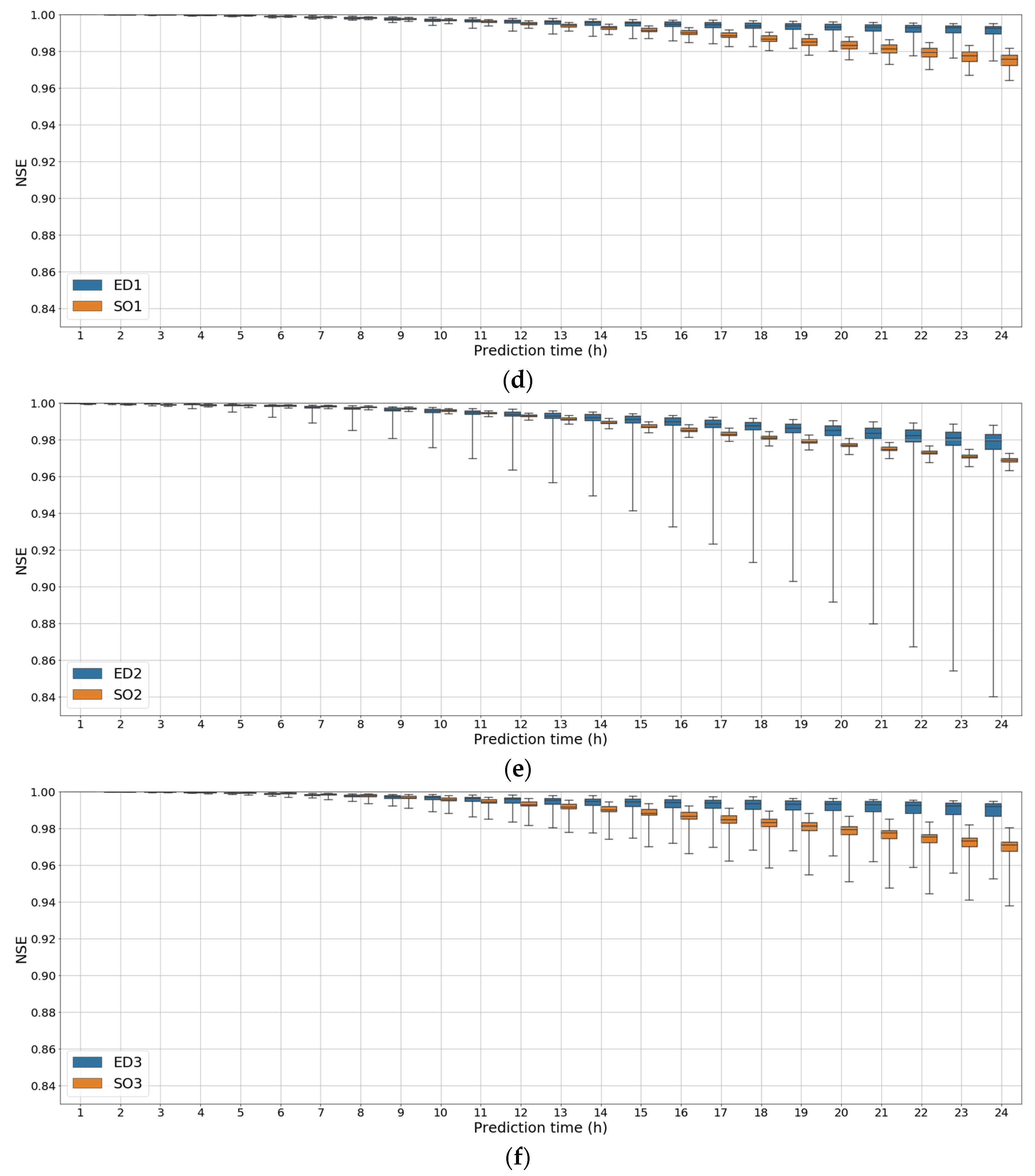
Figure 4 shows boxplots representing the results of each set of 20 ensemble learnings (obtained for making predictions) over a 24 h observation period. The figure shows the RMSE and NSE values for the LSTM SO1–SO3 and LSTM ED1-ED3 models using data obtained from 2 July to 23 September 2019. With the short-term predictions (approximately 10 h), no significant difference in the RMSE was observed, but the RMSE of the SO models increased as the predictions were generated over longer periods. This result was similar to that of a previous study [37].
Figure 4a–c shows that, especially with the LSTM SO model, changing the input variables did not lead to a significant reduction in errors. The LSTM ED1 model showed the smallest prediction error at 24 h, with an RMSE of 0.07. Compared with the SO2 and ED2 models, the errors were considerably lower with the SO3 and ED3 models, where the water-level difference was set as an input variable and the output was directly set as the water level. In addition, the smallest errors were found with the ED1 model (RMSE at 24 h of 0.07), where both water level and amount of change in water level were used as input variables. The SO1 and ED1 models had the lowest errors among three models of each type, SO and ED. The error between the models was 41%. The percentage decline in the RMSE values was larger in the ED models than in the SO models. In addition, the mean absolute error, which is used in the evaluation of hydrological models, was also evaluated, and the results were similar to the RMSE. Figure 4d–f presents boxplots for the computed NSE indexes, which were generated using the test data. The ED1 model presented the best results, with a maximum average NSE index of 0.99. The ED2 model showed large variations in the NSE values.
Therefore, the ED models were considered to provide higher accuracy, with both water level and water-level change, set as input variables instead of using either the water level or the water-level change as a single variable.
3.3. Relationship between Water-Level Changes and the Reservoir Capacity
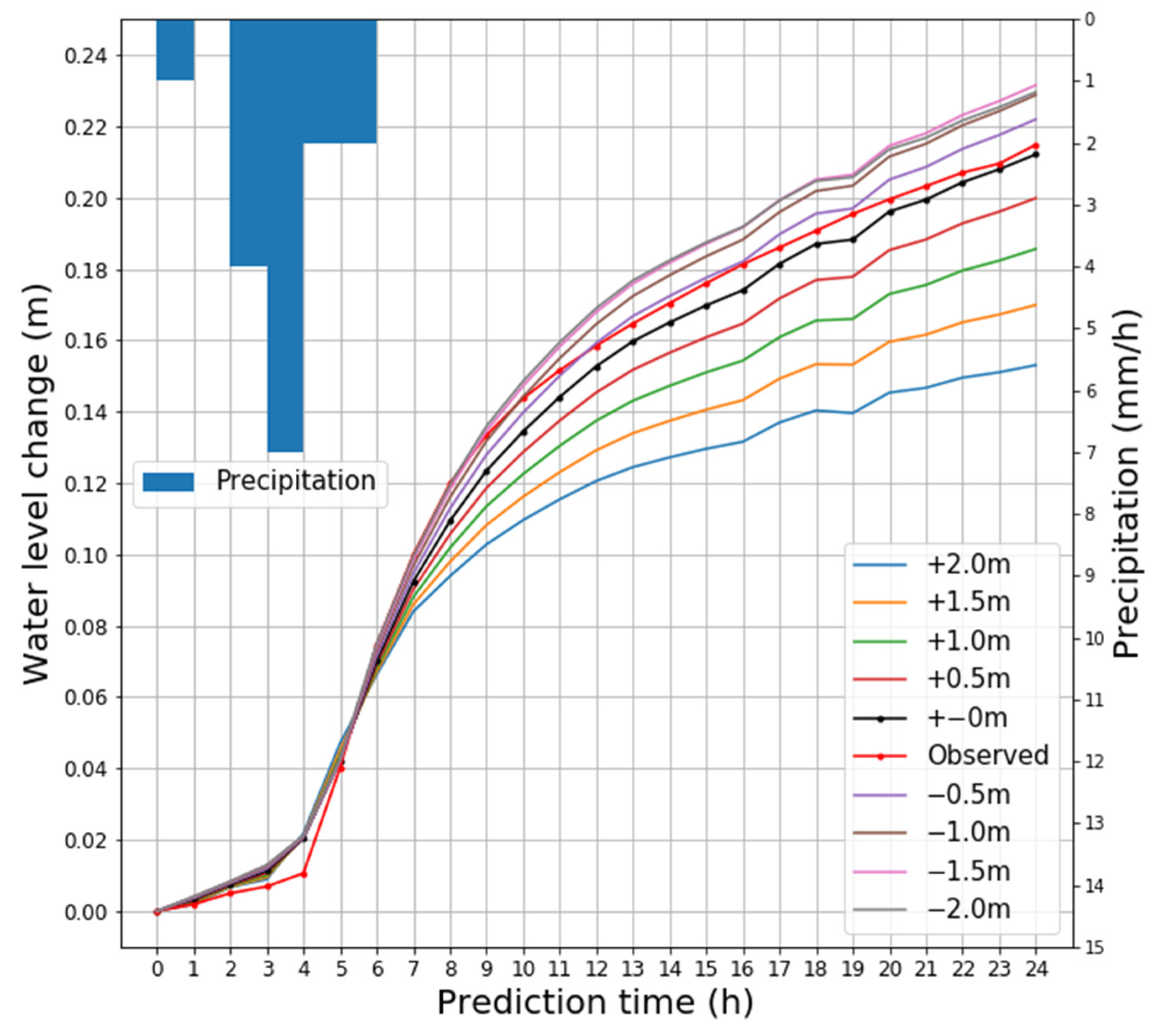
To examine the capability of our model to characterize the relationship between the simulated water level and the reservoir geometry, the changes in the water level from different initial water levels were computed. The rainfall data from 26 to 27 July 2019 (total rainfall of 16 mm, which is considered typical for the region) were used and computed using 0.5 m differences in the initial water level (Figure 5). The red and black lines represent the observed and simulated water-level changes, respectively. The other colored lines are the simulated water-level changes starting from the different initial water levels. The simulated water-level changes agreed with the observed water-level changes when the simulated and observed water levels were initially the same, and the results showed good reproducibility and accuracy. However, a small water-level change was predicted if the inflow started at a high water level, and a large water-level change was predicted if the inflow started at a low water level. The findings reveal that the LSTM ED models learned the relationship between the water level and water-level change and that, by knowing the cross-sectional geometry, they could estimate the inflow volume to the reservoir more accurately.
3.4. Assessment of the LSTM ED1 Model
An analysis was performed to further assess the predictions made using the LSTM ED1 model. The observed data were divided into 10 periods (Table 5). All data, except for one period assigned to the test data, were used for training and validation.
As the time lag between the start of rainfall events and water-level changes was approximately 3 h, a rainfall event shown in Table 5 was defined as one where the cumulative rainfall was 5 mm or more, and there was no rainfall for 4 h between the events. Overflows were observed from the spillway during periods 1, 9, and 10. The largest rainfall event (event 1) was observed from 4 to 6 July 2019 in period 1. The second-largest rainfall event occurred from 15 to 16 August 2019, in period 6. No overflow occurred during this period, and event 2 (occurring during period 6) was the largest rainfall event without overflow. The third-largest rainfall event occurred from 18 to 19 June 2020 in period 10 (event 3). No overflow occurred during the rainfall event.
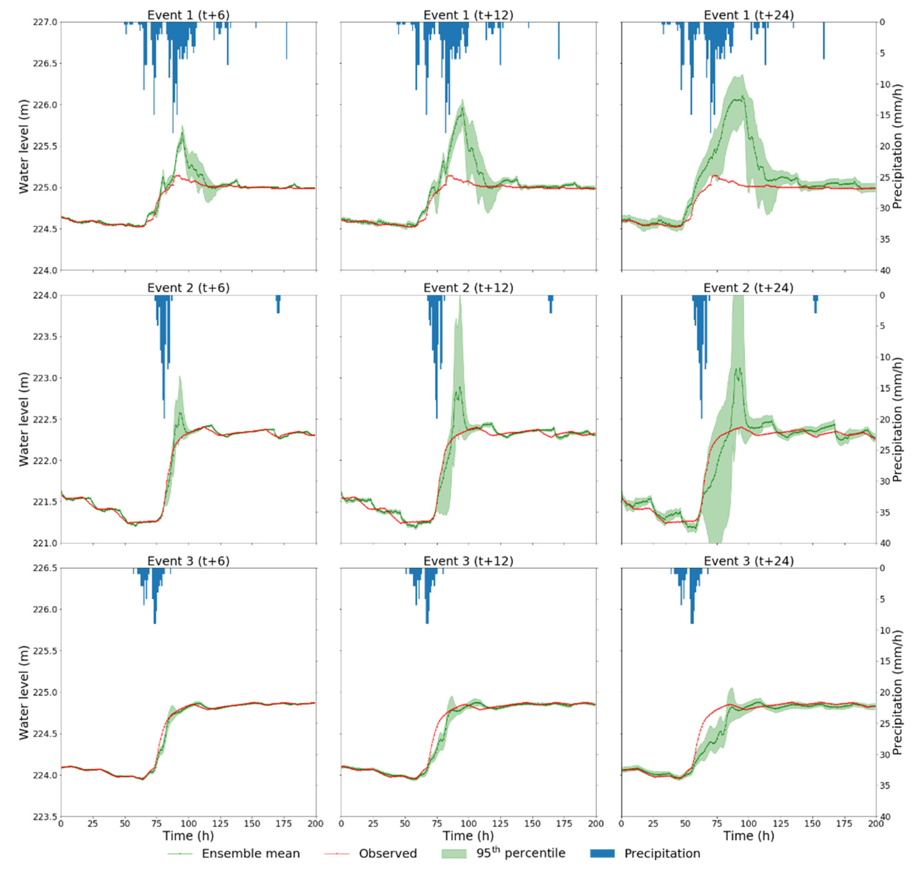
Figure 6 shows the three largest cumulative rainfall observations among the test data. The red dotted lines show the observed water levels, the green dotted lines show the averages of the predicted values after each ensemble learning, and the green shaded areas represent the ranges of the 95% confidence intervals of the predicted values after each learning of the ensemble member. Event 1 was a simulation of the largest rainfall event when the water reached full capacity and overflow occurred from the spillway. The range of the 95% confidence interval was larger when the water level fluctuated after rainfall, indicating the influence of the initial weighting in the LSTM model. This presented a prediction limitation when the rainfall intensity was larger than the range of the training data sets. In general, ensemble learning provides variable outputs, which indicates overfitting against the training dataset in deep learning [41]. This variation was caused by predictions made using an untrained rainfall event. Therefore, ensemble learning is a valuable technique for ascertaining the range of possible predicted water levels. Even when overflowing was above the spill level of 225 m, the observed water levels did not increase significantly, but the simulated results showed significant increases in the water levels. Only two overflow events were observed, which indicates that water-level fluctuations in the case of overflow could not be predicted well. This implies the need for more training data during overflow events.
Similarly, event 2 was the largest rainfall event without overflow. Although the prediction accuracy was better than that for event 1, the variation in the predicted value was larger when the water level fluctuated. In contrast, with event 3, the variation of the predicted value was considerably smaller than those of events 1 and 2, even during a large rainfall event with a small number of observations within the learning period, and the average predicted value after the ensemble was also close to the measured value.
Therefore, the LSTM ED models performed reasonably well when predicting water levels within the range of the training dataset. In the case of a rainfall event or overflow that fell outside the range of the training data values, the variation in prediction was significant. In any case, ensemble learning to assess the variation of outputs can feasibly improve the reliability of hydrological models by presenting a range of outputs.
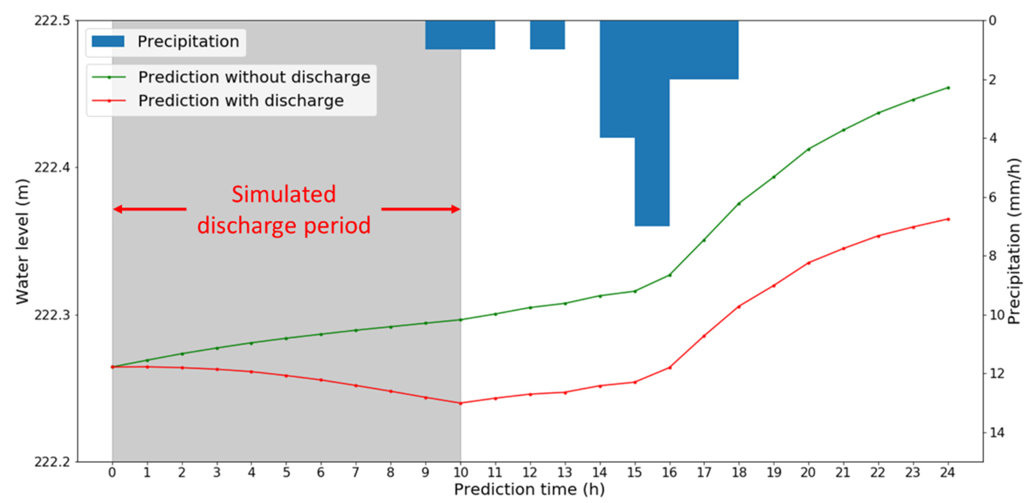
Figure 7 shows an example of the application of the LSTM ED model for different water levels, with or without a prior discharge before the rainfall event. The model provides helpful information regarding the timing and duration of discharge to enable rainwater collection without overflow from the reservoir. The model can quantitatively identify the effect of water discharge to increase the storage capacity before rainfall events occur.
4. Conclusions
To manage reservoir operations, it is important to store enough water for irrigation, while reducing the risk of flooding in the downstream area. The latter is especially important in the context of climate change, which may be associated with an increasing frequency of heavy rainfall. The application of deep learning models can be used for water-level predictions in reservoir management. These models are preferable over simple hydrological models. The LSTM model can potentially be used as a tool for predicting the water levels of small reservoirs with limited available hydrological variables for training, such as water level and rainfall and discharge events without the inflow and outflow data. Therefore, it may be possible to estimate the storage capacity and the area-volume-elevation curve without field surveys, based on the computed relationship between the water level and water-level change.
In this study, the output of a model with the encoder–decoder structure was compared with that of a common single-output LSTM model. The encoder–decoder structure in the LSTM model provided better simulation results, especially for predictions made over longer durations. In predicting the water level, our results showed similar trends to those of the previous study on runoff analysis using encoder–decoder [37]. After further analysis, the model accounted for the geometry of the reservoirs cross-section, based on time-dependent water-level information. Furthermore, the ensemble learning technique demonstrated a range of simulation errors that could be useful for understanding the ability of model predictions.
On the contrary, the LSTM ED model required more than two times more computation time than the LSTM SO model. As the LSTM ED has a more complex model structure than the LSTM SO, it is likely that more time was needed to train per time (1 Epoch) and converge the loss error. To reduce the learning cost, the extreme learning machine model has been studied in hydrological models [10,11,42], which could be applied in this study.
Furthermore, the ensemble learning technique demonstrated a range of simulation errors that could be useful for understanding the ability of model predictions. In addition, ensemble learning can assess the reliability of hydrological models by demonstrating the variation in simulated outputs. The errors can also be significant when the forecasted rainfall intensity is outside the range of the training data. To improve the accuracy, the accumulation of more training data for deep learning architectures or the application of transfer learning [43] should be considered for further studies. Management conditions of small reservoirs are rarely studied and are different from those of dams and large reservoirs. Therefore, further technological development and research focused on small reservoirs will be important.
Author Contributions
Conceptualization, T.K. and Y.M.; methodology, T.K., Y.M. and M.K.; software, T.K.; validation, T.K., M.K. and Y.M.; formal analysis, T.K.; resources, Y.M. and M.K.; data curation, Y.M. and M.K.; writing—original draft preparation, T.K.; writing—review and editing, Y.M. and A.Y.; visualization, T.K.; supervision, Y.M. and M.K.; project administration, Y.M.; funding acquisition, Y.M. and M.K. All authors have read and agreed to the published version of the manuscript.
Funding
This research was funded by the Rural Promotion Division of Nara Prefecture and KAKENHI, grant number 21H02309, from the Japan Society for the Promotion of Science.
Data Availability Statement
The data that support the findings of this study are available from the corresponding author upon reasonable request.
Acknowledgments
The authors acknowledge the support provided by Kitayamato Land Improvement District, especially Katsuda and Ariyama, who provided detailed information on the study area.
Conflicts of Interest
The authors declare no conflict of interest. The funders had no role in the design of the study; in the collection, analyses, or interpretation of data; in the writing of the manuscript, or in the decision to publish the results.
References
- Baup, F.; Frappart, F.; Maubant, J. Combining High-Resolution Satellite Images and Altimetry to Estimate the Volume of Small Lakes. Hydrol. Earth Syst. Sci. 2014, 18, 2007–2020. [Google Scholar] [CrossRef] [Green Version]
- Ogilvie, A.; Belaud, G.; Massuel, S.; Mulligan, M.; Le Goulven, P.; Malaterre, P.O.; Calvez, R. Combining Landsat Observations with Hydrological Modelling for Improved Surface Water Monitoring of Small Lakes. J. Hydrol. 2018, 566, 109–121. [Google Scholar] [CrossRef]
- Li, K.; Wan, D.; Zhu, Y.; Yao, C.; Yu, Y.; Si, C.; Ruan, X. The Applicability of ASCS_LSTM_ATT Model for Water Level Prediction in Small- and Medium-Sized Basins in China. J. Hydroinform. 2020, 22, 1693–1717. [Google Scholar] [CrossRef]
- Liu, M.; Huang, Y.; Li, Z.; Tong, B.; Liu, Z.; Sun, M.; Jiang, F.; Zhang, H. The Applicability of LSTM-KNN Model for Real-Time Flood Forecasting in Different Climate Zones in China. Water 2020, 12, 440. [Google Scholar] [CrossRef] [Green Version]
- Sajedi-Hosseini, F.; Malekian, A.; Choubin, B.; Rahmati, O.; Cipullo, S.; Coulon, F.; Pradhan, B. A Novel Machine Learning-Based Approach for the Risk Assessment of Nitrate Groundwater Contamination. Sci. Total Environ. 2018, 644, 954–962. [Google Scholar] [CrossRef] [Green Version]
- Kuo, Y.M.; Liu, C.W.; Lin, K.H. Evaluation of the Ability of an Artificial Neural Network Model to Assess the Variation of Groundwater Quality in an Area of Blackfoot Disease in Taiwan. Water Res. 2004, 38, 148–158. [Google Scholar] [CrossRef]
- Najafzadeh, M.; Homaei, F.; Mohamadi, S. Reliability Evaluation of Groundwater Quality Index Using Data-Driven Models. Environ. Sci. Pollut. Res. Int. 2021. [Google Scholar] [CrossRef]
- Barzkar, A.; Najafzadeh, M.; Homaei, F. Evaluation of Drought Events in Various Climatic Conditions Using Data-Driven Models and a Reliability-Based Probabilistic Model. Nat. Hazards 2021. [Google Scholar] [CrossRef]
- Belayneh, A.; Adamowski, J.; Khalil, B.; Ozga-Zielinski, B. Long-Term SPI Drought Forecasting in the Awash River Basin in Ethiopia Using Wavelet Neural Network and Wavelet Support Vector Regression Models. J. Hydrol. 2014, 508, 418–429. [Google Scholar] [CrossRef]
- Deo, R.C.; Şahin, M. Application of the Extreme Learning Machine Algorithm for the Prediction of Monthly Effective Drought Index in Eastern Australia. Atmos. Res. 2015, 153, 512–525. [Google Scholar] [CrossRef] [Green Version]
- Deo, R.C.; Tiwari, M.K.; Adamowski, J.F.; Quilty, J.M. Forecasting Effective Drought Index Using a Wavelet Extreme Learning Machine (W-ELM) Model. Stoch. Environ. Res. Risk Assess. 2017, 31, 1211–1240. [Google Scholar] [CrossRef]
- Deo, R.C.; Şahin, M. Application of the Artificial Neural Network model for prediction of monthly Standardized Precipitation and Evapotranspiration Index using hydrometeorological parameters and climate indices in eastern Australia. Atmos. Res. 2015, 161–162, 65–81. [Google Scholar] [CrossRef]
- Granata, F.; Di Nunno, F. Forecasting Evapotranspiration in Different Climates Using Ensembles of Recurrent Neural Networks. Agric. Water Manag. 2021, 255, 107040. [Google Scholar] [CrossRef]
- Yin, J.; Deng, Z.; Ines, A.V.M.; Wu, J.; Rasu, E. Forecast of Short-Term Daily Reference Evapotranspiration Under Limited Meteorological Variables Using a Hybrid Bi-Directional Long Short-Term Memory Model (Bi-LSTM). Agric. Water Manag. 2020, 242, 106386. [Google Scholar] [CrossRef]
- LeCun, Y.; Bengio, Y.; Hinton, G. Deep Learning. Nature 2015, 521, 436–444. [Google Scholar] [CrossRef] [PubMed]
- Pollack, J.B. Recursive Distributed Representations. Artif. Intell. 1990, 46, 77–105. [Google Scholar] [CrossRef]
- Hochreiter, S.; Schmidhuber, J. Long Short-Term Memory. Neural Comput. 1997, 9, 1735–1780. [Google Scholar] [CrossRef] [PubMed]
- Cho, K.; van Merrienboer, B.; Gülçehre, Ç.; Bougares, F.; Schwenk, H.; Bengio, Y. Learning Phrase Representations Using RNN Encoder-Decoder for Statistical Machine Translation. arXiv 2014, arXiv:1406.1078. [Google Scholar]
- Shewalkar, A.; Nyavanandi, D.; Ludwig, S.A. Performance Evaluation of Deep Neural Networks Applied to Speech Recognition: Rnn, LSTM and GRU. J. Artif. Intell. Soft Comput. Res. 2019, 9, 235–245. [Google Scholar] [CrossRef] [Green Version]
- Liu, P.; Qiu, X.; Huang, X. Recurrent Neural Network for Text Classification with Multi-Task Learning. In Proceedings of the 25th International Joint Conference on Artificial Intelligence, New York, NY, USA, 9–15 July 2016; pp. 2873–2879. [Google Scholar]
- Xu, J.; Chen, D.; Qiu, X.; Huang, X. Cached Long Short-Term Memory Neural Networks for Document-Level Sentiment Classification. In Proceedings of the Conference on Empirical Methods in Natural Language Processing, Austin, TX, USA, 1–5 November 2016. [Google Scholar]
- Huang, Z.; Xu, W.; Yu, K. Bidirectional LSTM-CRF Models for Sequence Tagging. arXiv 2015, arXiv:1508.01991. [Google Scholar]
- Schuster, M.; Paliwal, K.K. Bidirectional Recurrent Neural Networks. IEEE Trans. Signal Process. 1997, 45, 2673–2681. [Google Scholar] [CrossRef] [Green Version]
- Sutskever, I.; Vinyals, O.; Le, Q.V. Sequence to Sequence Learning with Neural Networks. In Proceedings of the 27th International Conference on Neural Information Processing Systems, Montreal, QC, Canada, 8–13 December 2014; Volume 2, pp. 3104–3112. [Google Scholar]
- Sit, M.; Demiray, B.Z.; Xiang, Z.; Ewing, G.J.; Sermet, Y.; Demir, I. A Comprehensive Review of Deep Learning Applications in Hydrology and Water Resources. Water Sci. Technol. 2020, 82, 2635–2670. [Google Scholar] [CrossRef] [PubMed]
- Hu, C.; Wu, Q.; Li, H.; Jian, S.; Li, N.; Lou, Z. Deep learning with a long short-term memory networks approach for rainfall-runoff simulation. Water 2018, 10, 1543. [Google Scholar] [CrossRef] [Green Version]
- Fu, M.; Fan, T.; Ding, Z.; Salih, S.Q.; Al-Ansari, N.; Yaseen, Z.M. Deep Learning Data-Intelligence Model Based on Adjusted Forecasting Window Scale: Application in Daily Streamflow Simulation. IEEE Access 2020, 8, 32632–32651. [Google Scholar] [CrossRef]
- Li, W.; Kiaghadi, A.; Dawson, C. High Temporal Resolution Rainfall–Runoff Modeling Using Long-Short-Term-Memory (LSTM) Networks. Neural Comput. Appl. 2021, 33, 1261–1278. [Google Scholar] [CrossRef]
- Xu, W.; Jiang, Y.; Zhang, X.; Li, Y.; Zhang, R.; Fu, G. Using Long Short-Term Memory Networks for River Flow Prediction. Hydrol. Res. 2020, 51, 1358–1376. [Google Scholar] [CrossRef]
- Kratzert, F.; Klotz, D.; Brenner, C.; Schulz, K.; Herrnegger, M. Rainfall-Runoff Modelling Using Long Short-Term Memory (LSTM) Networks. Hydrol. Earth Syst. Sci. 2018, 22, 6005–6022. [Google Scholar] [CrossRef] [Green Version]
- Zhang, D.; Lin, J.; Peng, Q.; Wang, D.; Yang, T.; Sorooshian, S.; Liu, X.; Zhuang, J. Modeling and Simulating of Reservoir Operation Using the Artificial Neural Network, Support Vector Regression, Deep Learning Algorithm. J. Hydrol. 2018, 565, 720–736. [Google Scholar] [CrossRef] [Green Version]
- Yang, S.; Yang, D.; Chen, J.; Zhao, B. Real-Time Reservoir Operation Using Recurrent Neural Networks and Inflow Forecast from a Distributed Hydrological Model. J. Hydrol. 2019, 579, 124229. [Google Scholar] [CrossRef]
- Hrnjica, B.; Bonacci, O. Lake Level Prediction Using Feed Forward and Recurrent Neural Networks. Water Resour. Manag. 2019, 33, 2471–2484. [Google Scholar] [CrossRef]
- Barzegar, R.; Aalami, M.T.; Adamowski, J. Short-Term Water Quality Variable Prediction Using a Hybrid CNN–LSTM Deep Learning Model. Stoch. Environ. Res. Risk Assess. 2020, 34, 415–433. [Google Scholar] [CrossRef]
- Zhu, S.; Luo, X.; Yuan, X.; Xu, Z. An Improved Long Short-Term Memory Network for Streamflow Forecasting in the Upper Yangtze River. Stoch. Environ. Res. Risk Assess. 2020, 34, 1313–1329. [Google Scholar] [CrossRef]
- Li, W.; Kiaghadi, A.; Dawson, C. Exploring the Best Sequence LSTM Modeling Architecture for Flood Prediction. Neural Comput. Appl. 2021, 33, 5571–5580. [Google Scholar] [CrossRef]
- Xiang, Z.; Yan, J.; Demir, I. A Rainfall-Runoff Model with LSTM-Based Sequence-to-Sequence Learning. Water Resour. Res. 2020, 56, e2019WR025326. [Google Scholar] [CrossRef]
- Kao, I.F.; Zhou, Y.; Chang, L.C.; Chang, F.J. Exploring a Long Short-Term Memory Based Encoder-Decoder Framework for Multi-Step-Ahead Flood Forecasting. J. Hydrol. 2020, 583, 124631. [Google Scholar] [CrossRef]
- Kingma, B.D.; Ba, L.J. Adam: A Method for Stochastic Optimization. arXiv 2014, arXiv:1412.6980v9. [Google Scholar]
- Opitz, D.; Maclin, R. Popular Ensemble Methods: An Empirical Study. J. Artif. Intell. Res. 1999, 11, 169–198. [Google Scholar] [CrossRef]
- Geron, A. Hands-On Machine Learning with Scikit-Learn, Keras & TensorFlow, 2nd ed.; O’Reilly Media, Inc.: Sebastopol, ON, Canada, 2019; p. 134. [Google Scholar]
- Saberi-Movahed, F.; Najafzadeh, M.; Mehrpooya, A. Receiving More Accurate Predictions for Longitudinal Dispersion Coefficients in Water Pipelines: Training Group Method of Data Handling Using Extreme Learning Machine Conceptions. Water Resour. Manag. 2020, 34, 529–561. [Google Scholar] [CrossRef]
- Pan, S.J.; Yang, Q. A Survey on Transfer Learning. IEEE Trans. Knowl. Data Eng. 2010, 22, 1345–1359. [Google Scholar] [CrossRef]
Figure 1.
Location of the Takayama Reservoir.

Figure 2.
Structures of the LSTM SO (top diagram) and LSTM ED (bottom diagram) models for reservoir water level prediction.
Figure 2.
Structures of the LSTM SO (top diagram) and LSTM ED (bottom diagram) models for reservoir water level prediction.

Figure 3.
Water levels during the study.

Figure 4.
Comparison of the RMSE and NSE values using different output methods for ensemble learning when performing 24 h simulations. (a–c) show RMSEs of the output values following simulations with three different models (types 1, 2, and 3, respectively) for both LSTM SO and LSTM ED models. Panels (d–f) show NSE indexes obtained using outputs with the same model types.


Figure 5.
Water-level changes with different initial water levels (from −2.0 m to 2.0 m), using the LSTM ED1 model.
Figure 5.
Water-level changes with different initial water levels (from −2.0 m to 2.0 m), using the LSTM ED1 model.

Figure 6.
Observed and predicted water levels for the LSTM ED1 simulations at 6, 12, or 24 h in events 1 to 3. The 95th percentiles for the ensemble member predictions are shown with light green shading.
Figure 6.
Observed and predicted water levels for the LSTM ED1 simulations at 6, 12, or 24 h in events 1 to 3. The 95th percentiles for the ensemble member predictions are shown with light green shading.

Figure 7.
Example application of the developed model for predicting water-level changes when water was released before a forecasted rainfall event.
Figure 7.
Example application of the developed model for predicting water-level changes when water was released before a forecasted rainfall event.


Table 1.
Basic specifications of the Takayama Reservoir.
| Capacity | Surface Area | Catchment Area |
| 580,000 m3 | 90,000 m2 | 2.3 km2 |
| Beneficiary Area | Embankment Height | Embankment Length |
| 530 ha | 23 m | 135 m |
Table 2.
Types of models developed and their input and output variables.
| Model Type | Model Name | Input Variable | Output Variable |
|---|---|---|---|
| LSTM Single-output | SO1 | Precipitation (mm/h) Discharge event (0 or 1) Water level (m) Water-level change (m/h) | Water-level change (m) |
| SO2 | Precipitation (mm/h) Discharge event (0 or 1) Water level (m) | Water level (m) | |
| SO3 | Precipitation (mm/h) Discharge event (0 or 1) Water-level change (m/h) | Water-level change (m) | |
| LSTME ncoder-decoder | ED1 | Precipitation (mm/h) Discharge event (0 or 1) Water level (m) Water-level change (m/h) | Water-level change (m) |
| ED2 | Precipitation (mm/h) Discharge event (0 or 1) Water level (m) | Water level (m) | |
| ED3 | Precipitation (mm/h) Discharge event (0 or 1) Water-level change (m/h) | Water-level change (m) |
Table 3.
Parameters of the developed models.
| Type Name | Hidden Unit | Batch Size | Optimizer | Loss Function | Epochs (Early Stopping) | Input Length (h) | Output Length (h) |
|---|---|---|---|---|---|---|---|
| LSTM SO1 to SO3 | 20 | 64 | Adam | Mean squared error | 150 | 25 | 1 |
| LSTM ED1 to ED3 | 20 | 64 | Adam | Mean squared error | 200 | 25 | 24 |
Table 4.
Summary of data obtained from Takayama Reservoir during the study.
| Item | Counts | Mean | Standard Deviation | Max | Min | Total Discharge Time |
|---|---|---|---|---|---|---|
| Water level (m) | 17,690 | 221.86 | 1.95 | 225.14 | 218.35 | - |
| Precipitation (mm/h) | 18,072 | 0.12 | 0.76 | 28.00 | 0.00 | - |
| Discharge | 17,690 | - | - | - | - | 6171 |
Table 5.
Summary of rainfall and water level during the divided periods used for testing the LSTM ED1 model.
Table 5.
Summary of rainfall and water level during the divided periods used for testing the LSTM ED1 model.
| Period Number | Period | Rainfall Event | Water Level | ||||
|---|---|---|---|---|---|---|---|
| Number of Events | Max Rainfall (mm/event) | Mean Rainfall (mm/event) | Max (m) | Min (m) | Mean (m) | ||
| 1 | 1 Jul. 2018–16 Sep. 2018 | 11 | 213.0 | 37.9 | 225.14 | 222.25 | 223.74 |
| 2 | 16 Sep. 2018–3 Dec. 2018 | 9 | 33.0 | 18.8 | 224.01 | 218.40 | 221.05 |
| 3 | 3 Dec. 2018–19 Feb. 2019 | 7 | 15.0 | 8.6 | 219.33 | 218.97 | 219.17 |
| 4 | 19 Feb. 2019–8 May 2019 | 10 | 26.0 | 12.9 | 222.40 | 219.28 | 220.75 |
| 5 | 8 May 2019–25 Jul. 2019 | 14 | 33.0 | 14.0 | 222.65 | 220.21 | 221.39 |
| 6 | 25 Jul. 2019–11 Oct. 2019 | 13 | 102.0 | 18.7 | 223.30 | 221.24 | 222.63 |
| 7 | 11 Oct. 2019–28 Dec. 2019 | 9 | 61.0 | 20.6 | 223.25 | 218.35 | 220.47 |
| 8 | 28 Dec. 2019–15 Mar. 2020 | 13 | 19.0 | 11.8 | 222.82 | 219.89 | 221.45 |
| 9 | 15 Mar. 2020–1 Jun. 2020 | 11 | 25.0 | 12.6 | 225.09 | 222.82 | 224.57 |
| 10 | 1 Jun. 2020–22 Jul. 2020 | 11 | 70.0 | 25.9 | 225.09 | 223.43 | 224.57 |
Publisher’s Note: MDPI stays neutral with regard to jurisdictional claims in published maps and institutional affiliations. |
© 2021 by the authors. Licensee MDPI, Basel, Switzerland. This article is an open access article distributed under the terms and conditions of the Creative Commons Attribution (CC BY) license (https://creativecommons.org/licenses/by/4.0/).
Share and Cite
MDPI and ACS Style
Kusudo, T.; Yamamoto, A.; Kimura, M.; Matsuno, Y. Development and Assessment of Water-Level Prediction Models for Small Reservoirs Using a Deep Learning Algorithm. Water 2022, 14, 55. https://doi.org/10.3390/w14010055
AMA Style
Kusudo T, Yamamoto A, Kimura M, Matsuno Y. Development and Assessment of Water-Level Prediction Models for Small Reservoirs Using a Deep Learning Algorithm. Water. 2022; 14(1):55. https://doi.org/10.3390/w14010055
Chicago/Turabian StyleKusudo, Tsumugu, Atsushi Yamamoto, Masaomi Kimura, and Yutaka Matsuno. 2022. "Development and Assessment of Water-Level Prediction Models for Small Reservoirs Using a Deep Learning Algorithm" Water 14, no. 1: 55. https://doi.org/10.3390/w14010055
Note that from the first issue of 2016, this journal uses article numbers instead of page numbers. See further details here.