Nonstationary Bayesian Modeling of Extreme Flood Risk and Return Period Affected by Climate Variables for Xiangjiang River Basin, in South-Central China

Abstract

The accurate design flood of hydraulic engineering is an important precondition to ensure the safety of residents, and the high precision estimation of flood frequency is a vital perquisite. The Xiangjiang River basin, which is the largest river in Hunan Province of China, is highly inclined to floods. This paper aims to investigate the annual maximum flood peak (AMFP) risk of Xiangjiang River basin under the climate context employing the Bayesian nonstationary time-varying moment models. Two climate covariates, i.e., the average June-July-August Artic Oscillation and sea level pressure in the Northwest Pacific Ocean, are selected and found to exhibit significant positive correlation with AMFP through a rigorous statistical analysis. The proposed models are tested with three cases, namely, stationary, linear-temporal and climate-based conditions. The results both indicate that the climate-informed model demonstrates the best performance as well as sufficiently explain the variability of extreme flood risk. The nonstationary return periods estimated by the expected number of exceedances method are larger than traditional ones built on the stationary assumption. In addition, the design flood could vary with the climate drivers which has great implication when applied in the context of climate change. This study suggests that nonstationary Bayesian modelling with climatic covariates could provide useful information for flood risk management.

1. Introduction

Extreme flood events with immediate and widespread devastation on natural systems and society have been extensively studied over recent decades [1]. The flood frequency analysis is a critical and effective tool to estimate flood risk and is commonly accepted by hydrologists. In recent decades, with climate change and anthropogenic activities, the stationary flood frequency analysis method is frequently questionable relative to the heterogeneous flood population; meanwhile, the nonstationary extreme flood risk analysis with various methodological frameworks has been extensively explored over recent decades. Among these approaches, the extreme flood risk analysis considering environmental factors could assist decision makers and engineers to better understand the nonstationary behaviors of extreme flood events and to take flood control measures quickly.

In general, extreme flood events have occurred all around the world, with a wide variety of regional characteristics. Among the several nonstationary flood frequency approaches, the time-varying moment method is widely utilized. Through incorporating factors into the covariates of model parameters, the time-varying moment method could quantify and even forecast the variation of extreme flood risks under changing environments [2,3,4,5,6]. For instance, Lopez and Frances (2013) applied the generalized additive models for location, scale and shape (GAMLSS) on flood risk impacted by multiple climate indices such as Arctic Oscillation (AO), North Atlantic Oscillation (NAO), Mediterranean Oscillation and so on [7]. Ficchi et al. (2021) reported that the Indian Ocean Dipole (IOD) and Tropical South Atlantic climate mode are equally as important as El Nino-Southern Oscillation (ENSO) for driving changes in the frequency of impactful floods across Africa [8]. Zhou (2020) quantified the contributions of changing climate and reservoir storage on the nonstationarity in flood risks worldwide [9]. Zhang et al. (2015) estimated the annual maximum stream-flow quantiles linearly conditional on Pacific Decadal Oscillation (PDO) in South China [10]. Kundzewicz et al. (2019b) reviewed the linkages between climate variability and water-abundance like high river discharge, flood magnitude and flood loss across the world [11] and Kundzewicz et al. (2020) analyzed the non-stationarity of flood frequency over China [12]. Not only the standard climate indices with limited spatial climate information as climate forcing on extreme flood risk, but also the large-scale ocean-atmosphere fields play a critically important role in the interpretation of the nonstationary behavior on flood. Zeng et al. (2017) used sea surface temperature anomaly (SSTa) in Northern Indian Ocean and Western Pacific Ocean incorporated into the location and scale parameters of lognormal distribution and general extreme value distribution (GEV) to forecast the flood risk in North China using a Bayesian framework [13]. Renard and Lall (2014) employed the large-scale oceanic fields to effectively predict the flood risk in regional nonstationary flood frequency [14]. In this paper, the large-scale climate patterns including the standard climate variability indices and oceanic or atmospheric fields are considered to access the climatic drivers of nonstationary extreme flood frequency and design flood in Xiangjiang River basin in South-Central China.

Indeed, the time-varying moment method is widely proposed to implement the nonstationary flood frequency analysis under the changing environment. Nevertheless, the flood quantiles or return periods varying with covariates yearly is not convincing and convenient in real-world applications. For the sake of accommodating nonstationary conditions, several hydrologic design flood methods [15] have been proposed in recent years, such as the expected waiting time (EWT) [16,17], the expected number of exceedances (ENE) [18,19], design life level (DLL) [20] and equivalent reliability (ER) [21]. Yan et al. (2017) compared and applied the above four design flood methods on annual maximum flood series in several basins [15]. The results indicated that ENE, DLL and ER yielded very similar design flood values for both increasing and decreasing trends. Yan et al. (2020) focused on applying the EWT method to estimate the design flood quantiles and proposed the extrapolation time to guarantee the convergence of the EWT [22]. Given the advantages and disadvantages of these methods [23,24], we choose the ENE method to calculate design floods under a changing climate and the estimated stationary design floods serve as a benchmark for comparison.

The Xiangjiang River is the largestof Hunan Province in South-Central China and its basin is the dominating inflow basin of Dongting Lake, which is the second largest freshwater lake in China, located in the Yangtze River basin. Characterized by the subtropical monsoon climate, the Xiangjiang River basin is highly prone to floods during the summer season from June to August. Mao et al. (2000) reported that the middle and lower reaches of the Xiangjiang River basin have experienced 29 flooding disasters during the years from 1949 to 1998, which is about one flood per 1.7 years on average [25]. Extreme pluvial floods happened in the years of 1954, 1976, 1994, 1996 and 1998. In July 2006, the Southern Hunan Province suffered a 500-year rainstorm caused by the Severe Tropical Storm Bilis and the triggered torrential flood brought casualties and economic loss exceeding 78 hundred million China Yuan [26]. In the summer of 2017, the main stream of the Xiangjiang River basin reached a historic recorded water level due to the influence of a heavy rainfall combined with the flood control measures that were largely relying on the embankment on the riverside. Therefore, extreme flood risk analysis under changing climate is a vital and urgent issue for the Xiangjiang River basin. Although a great amount of research on the extreme flood occurrence probability and design flood under changing climate in the Yangtze River basin has been undertaken, very few studies have been conducted on extreme flood/rainfall frequency analysis triggered by large-scale climate patterns in the Xiangjiang River Basin.

In the Xiangjiang River basin, as floods are primarily driven by abundant precipitation in the wet seasons, we focus on identifying the significant climate covariates for extreme flood peaks and quantitatively estimating the climate contribution to the probability of extreme flood events and design flood using the nonstationary modeling framework. Moreover, in at-site extreme flood frequency analysis, there generally exists relatively large uncertainty. This is especially the case for the probability distribution with more parameters. Hence, the Bayesian statistical model is developed to access the uncertainty of flood risks and the updated return periods in stationary and nonstationary contexts. The results will provide a protocol for the selection of covariates in terms of nonstationary conditions and also show implications for controlling floods and reinforcing the projects of engineers and scientists.

The paper is organized as follows. In Section 2, we describe the study area, the data set and the screening process for selecting climatic factors. Section 3 presents the methodologies and theoretical analysis of the nonstationary model construction, along with a brief description of Bayesian modeling framework and nonstationary hydrologic design method. The results and discussions are demonstrated in Section 4. Finally, the article concludes in Section 5.

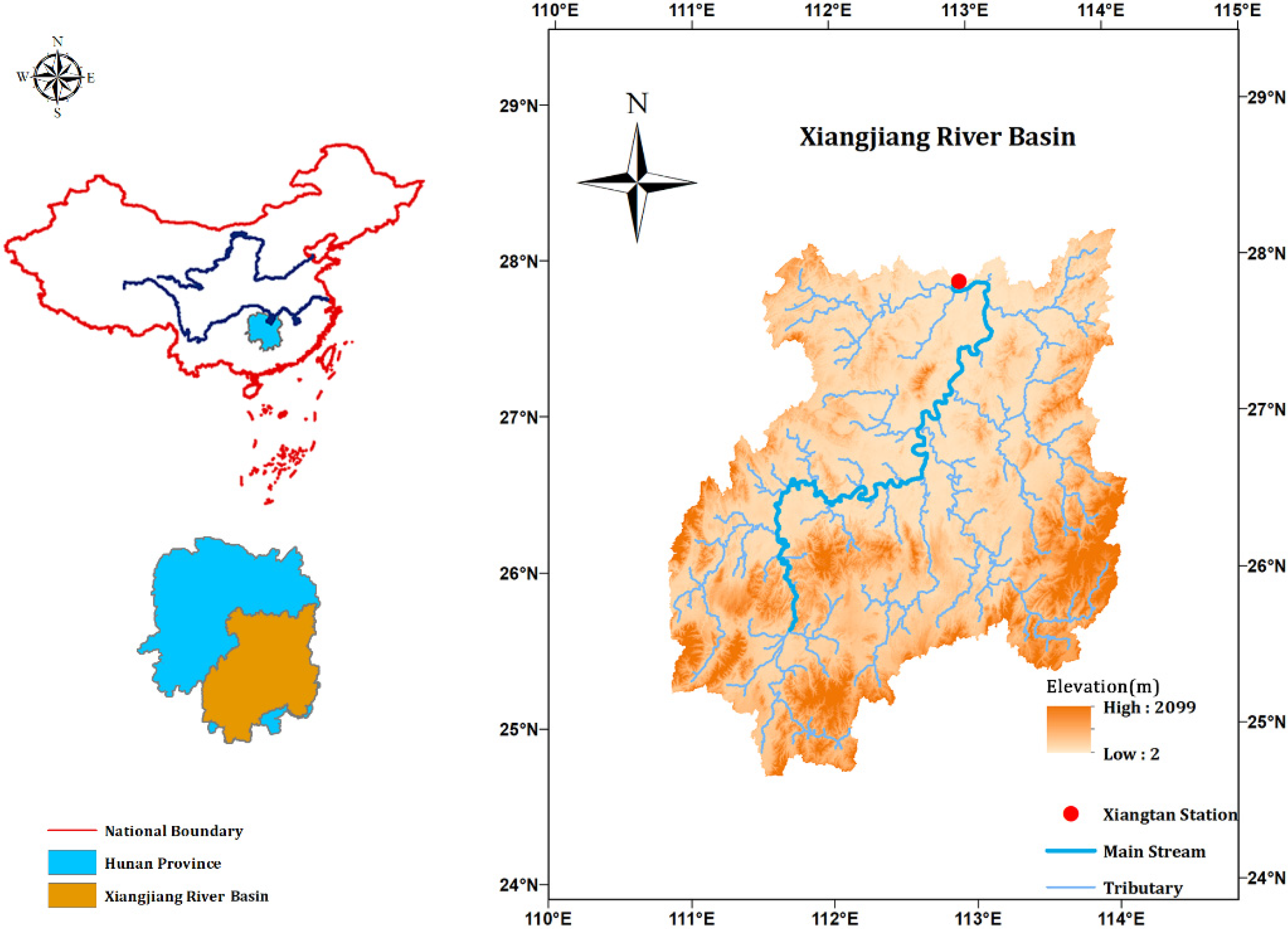
2. Study Area and Data

The Xiangjiang River basin (Figure 1) is bound by 24°–29° N and 110°30′–114° E in South-Central China with a drainage area of 94,660 km² and a total length of 856 km. Due to the southeast monsoon humid climate in summer, the basin is frequently exposed to extraordinary rainstorm with average annual precipitation ranging from 1200 to 1700 mm and large floods in the rainy season (April to September) leading to high water levels. Because of the low-lying terrain in the middle and lower reaches of the Xiangjiang River, the metropolitan area of Chang-Zhu-Tan, which is the most important economic belt in Hunan Province, does not have appropriate conditions for building a large dam and can, therefore, only rely on the construction of riverside dikes for flood control. In recent years, rainstorm flooding of the Xiangjiang River has continuously reached historic records, having a strong negative impact on the residents. Therefore, analysis of flood risk and uncertainty is extremely important for basin-wide flood risk reduction and management.

2.1. Extreme Flood

The annual maximum flood peak series (AMFP), spanning the period of 1959–2017 and measured by the Xiangtan hydrological station (Figure 1) as well as the outflow control station of the Xiangjiang River basin, were collected from the Hydrology and Water Resources Survey Bureau of Hunan Province.

In general, the time-varying characteristic of AMFP is investigated using the Mann–Kendall test and the results indicate that there is no significant trend. Nevertheless, the Xiangjiang River Basin has abundant flow as rainfall is the main source. Annual extreme flood events, taking place during the flood season (June-July-August-September, JJAS), are generally due to heavy rainstorms corresponding to various induced climatic factors. Hence, it is interesting and important to conduct an impact assessment of the climate variables on the flood peak risks in the Xiangjiang River basin.

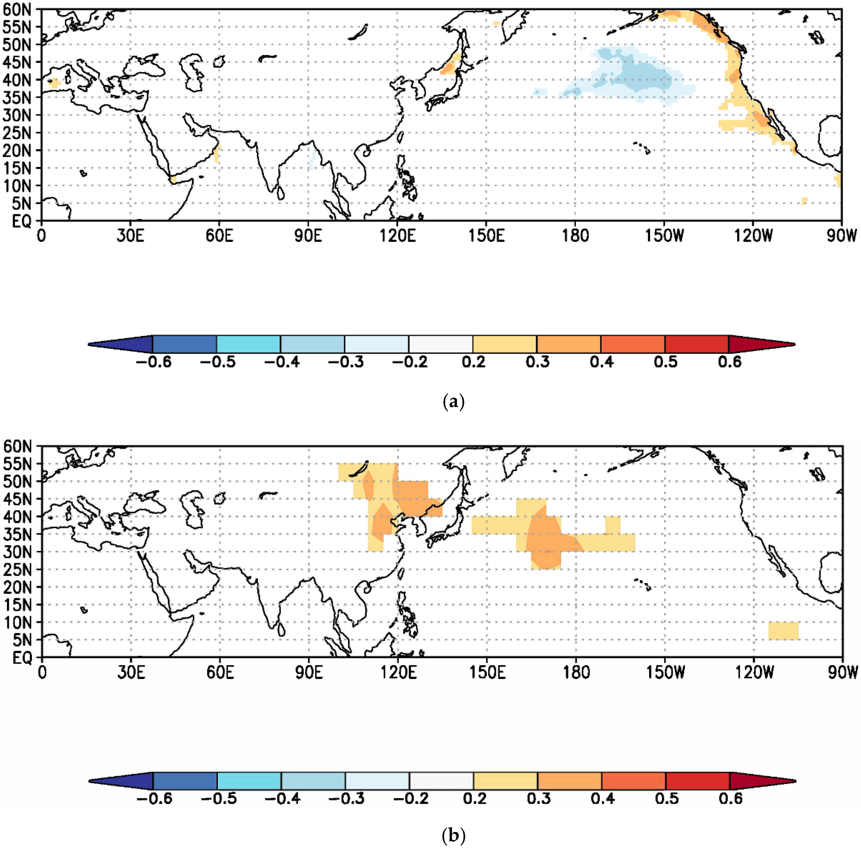
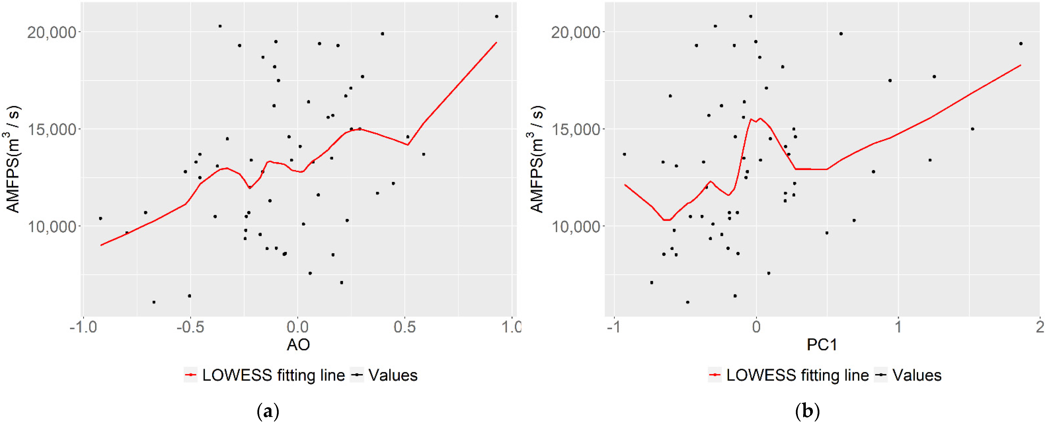
2.2. Identification of Significant Climate Factors

Identifying appropriate factors is a crucial step to better explain the variation in extreme flood frequency and to significantly improve the performance of nonstationary modeling. Slowly varying climate conditions associated with oceanic temperature may influence the development of the monsoon systems that affect the Xiangjiang River basin in the JJAS season. Thus, in this section, we explore the potential climate impact factors, involving various large-scale low-frequency climate indices: sea surface temperature anomaly (SSTa) conditions extracted from the Hadley Center SST dataset on a 1° × 1°grid [27]; and sea level pressure anomalies (SLPa) extracted from the Hadley Centre’s mean sea level pressure data set on a 5° × 5°grid [28]. Simultaneously, as suggested by Zeng et al. (2017) [13], we propose a stepwise selection method to screen the potential climate drivers employing rank correlation and a generalized linear model (GLM) to identify the orthogonal factors which have the best significant correlation with AMFP and the best flood risk modelling performance.

It is extensively recognized that the large-scale atmospheric circulation pattern climate indices, such as ENSO, including Southern Oscillation Index (SOI), Niño 3.4, Niño 12, Niño 3 and Niño 4, PDO, NAO and AO, can significantly influence hydrological variables (flood and precipitation) in China [29,30,31]. Then, the above climate indices, SLPa and SSTa, are selected as the possible influencing drivers. A three-month moving average from January to February of the next year of all the candidate factors are computed to access the rank correlation with AMFP using the Spearman rank correlation test. The results in

Table 1. Spearman rank correlation results between climate indices and AMFP ($\alpha =0.05$).

Climate Indices	Coefficient	JFM	FMA	MAM	AMJ	MJJ	JJA	JAS	ASO	SON	OND
Niño3	Rho	0.16	0.10	0.04	−0.05	−0.09	−0.12	−0.12	−0.11	−0.08	−0.06
	p-value	0.23	0.45	0.74	0.74	0.51	0.38	0.38	0.42	0.55	0.67
Niño4	Rho	0.09	0.09	0.05	0.02	−0.06	−0.11	−0.15	−0.15	−0.16	−0.15
	p-value	0.50	0.49	0.71	0.86	0.66	0.43	0.26	0.26	0.22	0.26
Niño3.4	Rho	0.14	0.11	0.07	0.04	−0.06	−0.11	−0.15	−0.15	−0.13	−0.11
	p-value	0.28	0.41	0.59	0.76	0.67	0.39	0.26	0.26	0.31	0.40
Niño12	Rho	0.10	0.04	−0.01	−0.03	−0.06	−0.05	−0.02	0.05	0.05	0.04
	p-value	0.47	0.74	0.94	0.82	0.64	0.73	0.86	0.72	0.71	0.77
SOI	Rho	−0.16	−0.18	−0.13	−0.02	0.08	0.04	0.03	0.05	0.10	0.17
	p-value	0.24	0.17	0.31	0.89	0.56	0.77	0.83	0.74	0.47	0.19
NAO	Rho	0.13	−0.02	−0.22	−0.05	0.04	0.10	−0.08	−0.24	−0.24	−0.17
	p-value	0.32	0.91	0.09	0.73	0.78	0.45	0.55	0.06	0.06	0.20
PDO	Rho	0.24	0.19	0.11	0.10	0.04	0.02	−0.07	−0.08	−0.06	−0.03
	p-value	0.07	0.16	0.41	0.47	0.74	0.87	0.61	0.55	0.64	0.82
AO	Rho	0.19	0.11	−0.02	0.04	0.19	0.32	0.15	−0.14	−0.23	−0.14
	p-value	0.16	0.41	0.87	0.78	0.16	0.01	0.26	0.28	0.08	0.29

Note: JFM, FMA, MAM, AMJ and so on, are the three-month moving average values, respectively. For example, JJA, means the average value of the climate variable during June, July and August. The value with underline “_” represents the p value less than 0.05.

illustrate that the Spearman rank correlations between flood peak series and the ENSO, PDO, NAO are typically low and statistically non-significant. In addition, it demonstrates that only AO during JJA has significant positive rank correlation with AMFP. Strong teleconnection between precipitation/flood anomalies in the Yangtze River Basin and AO has been found in previous studies [29,32,33]. In addition, the findings of Yang (2011) and Gong and Wang (2003) suggested that a statistically significant positive correlation was detected between the AO and the precipitation over South China [34,35]. The AO, a primary mode of internal atmospheric dynamics over the extratropical northern hemisphere with a quasi-barotropic structure from the surface to the lower stratosphere, exerts great influences on global climate processes [36,37]. Consequently, the average AO from June to August is used as the first candidate factor.

With respect to the SLPa and SSTa, we utilize the correlation map [14] to determine the climatic factors. Figure 2a,b demonstrates the Spearman rank correlation between AMFP and the SSTa fields during JFM, and SLPa fields during JJA, respectively. We find that the JFM SSTa blue region (35° N–45° N, 150° W–170° W) reveals significant negative rank correlation with AMFP. In contrast, the two JJA SLPa orange regions (one is the continent region for 35° N–50° N, 110° E–135° E called SLPa1, another is the ocean for 25° N–40° N, 165° E–180° E named SLPa2) show significant positive rank correlation with AMFP. A principal component analysis (PCA) is employed to acquire a set of orthogonal factors on the above JFM SSTa, JJA SLPa1 and JJA SLPa2, respectively, since the large-scale climate variables with fields may be mutually correlated.

Therefore, three sub-sets of the ten leading principal components named by SSTa-PCs, SLPa1-PCs and SLPa2-PCs, respectively, and the average seasonal (JJA) AO are then considered as potential factors. These factors are further investigated to search the best combination by a generalized linear model (GLM) [13] with an extended leave-one-out cross validation (LOOCV) method implemented by the R package ‘bestglm’ [38] to choose the candidate climatic factors. For the sake of obtaining the best combination, we propose four GLMs: (1) the first GLM with the SSTa-PCs and AO; (2) the second GLM with SLPa1-PCs and AO; (3) the third GLM with SLPa2-PCs and AO; and (4) the last GLM with AO and the five leading PCs of SLPa1 and SLPa2. The optimal combination, composited by JJA AO and the first principal component accounting for 73.52% of the total variance of JJA SLPa2 region (denoted by SLPa2-PC1), is selected as it has the minimum R square value (the method theory can be referred to [38]). The scatter plots between JJA AO, JJA SLPa2-PC1 and AMFP are displayed in Figure 3 and their Spearman correlations are exhibited in

Table 2. Spearman correlation coefficients between climatic factors and AMFP.

Climate Factors	AO	SLPa2-PC1
Coefficients	0.32	0.35
p-value	0.01	0.006

.

Flooding of the Xiangjiang river basin in Central and Southern China is greatly impacted by the East Asian summer monsoon, which is driven by the SLP contrast between the Asian low and the Pacific high [39]. The positive correlation teleconnection between JJA SLPa2 and the summer flood in the Xiangjiang river basin suggests that the high pressure in the Pacific Ocean would lead to more water vapor transporting to the Xiangjiang river basin [40]. In consequence, the abovementioned average seasonal JJA AO and SLPa2-PC1 are capable of describing the observed variability of extreme flood events in the Xiangjiang River basin and are selected to reflect the impact of climate change on flood risk.

3. Methodology

3.1. Choice of Distribution

After ascertaining the climate drivers for the flood peaks generation, the next step is to quantify the flood risk changes with climate change. According to the review of a suitable probability distribution function on flood frequency analysis by [41,42] and all the pdfs of the Interagency Advisory Committee on Water Data (1982) [43], the two-parameter log normal LN2 and log Pearson type III are the only two distributions which do not exhibit significant bias in observed flood frequencies. Since LN2 in nonstationary condition is more parsimonious and is one of the most widely used distributions in hydrology, we choose the LN2 to fit the observed AMFP. The probability density function (PDF) is given by:

$$f(x|\mu ,\sigma )=\frac{1}{x\sigma \sqrt{2\pi }}\exp \left[-\frac{{(\ln x-\mu )}^2}{2{\sigma }^2}\right],x>0;\sigma >0$$

(1)

where $\mu$ and $\sigma$ are the location and scale parameters, respectively. To capture the climate impact, we develop climate variables incorporated into the estimates of the location and scale parameters.

3.2. Nonstationary Models Construction

In the nonstationary condition, the parameters $\mu$ (mean, location) and $\sigma$ (standard deviation, scale) of LN2 are made time-dependent by incorporating time or climatic factors as covariates [44]. In this study, in consideration of the significant linear relationship shown in scatter plots in Figure 3 and the parsimonious nonstationary modelling requirement, the parameters are selected to be the linear functions of covariates. In addition, given the AMFP doesn’t exhibit a significant trend, the stationary condition (all parameters in the LN2 are constant) and the nonstationary model using time as the covariate are taken as the benchmarks to conduct the comparative analysis. Consequently, the stationary and nonstationary combinations of parameters are given as follows.

Case 1. Time-invariant model. All the parameters are kept constant, which is represented by

$${\mathrm{LN}}_{\mathrm{S}}:\mu ={\mu }_0,\ln (\sigma )={\sigma }_0$$

(2)

Case 2. Linear temporal model. Only the parameter location is modeling as a function of time, or both the location and scale linearly vary with time. The two models are given by

$$\mathrm{LNt}\text{-}1:\mu ={\mu }_0+{\mu }_{1}t,\ln (\sigma )={\sigma }_0$$

(3)

$$\mathrm{LNt}\text{-}2:\mu ={\mu }_0+{\mu }_{1}t,\ln (\sigma )={\sigma }_0+{\sigma }_{1}t$$

(4)

Case 3. Climate-informed model. Nonstationarity is incorporated by allowing the location, or both the location and scale parameters, to vary as a function of climatic factors (JJA AO and SLPa2-PC1). The models are illustrated as follows,

$${\mathrm{LN}}_{\mathrm{C}}\text{-}1:\mu ={\mu }_0+{\mu }_1\ast \mathrm{AO}+{\mu }_2\ast \mathrm{PC}1,\ln (\sigma )={\sigma }_0$$

(5)

$${\mathrm{LN}}_{\mathrm{C}}\text{-}2:\mu ={\mu }_0+{\mu }_1\times \mathrm{AO}+{\mu }_2\times \mathrm{PC}1,\ln (\sigma )={\sigma }_0+{\sigma }_1\times \mathrm{AO}+{\sigma }_2\times \mathrm{PC}1$$

(6)

where in the Case 1, Case 2 and Case 3, the letters s, t and c represent the stationary, time-varying and climate-based models respectively. The ${\mu }_i(i=0,1,2)$ and ${\sigma }_i(i=0,1,2)$ are the estimated regression parameters. For the sake of obtaining the positive values of $\sigma$, we use the natural logarithm $\ln \sigma$.

3.3. Bayesian Inference

In this study, we use a Bayesian inference framework to fit observed AMFP to the LN2 distribution. Bayesian-based Markov Chain Monte Carlo (MCMC) sampling with the No-U-Turn sampler variant of Hamiltonian Monte Carlo algorithm [45,46] in the RStan [47] is implemented to estimate the regression parameters associated with the covariates. The Bayesian-based MCMC approach provides full posterior distribution estimates of the parameters, which incorporate constructions from noninformative prior distributions and four chains of 10,000 iteration lengths in a statistically consistent way. The Bayesian theory rule is shown below,

$$f(\theta |X)\propto f(X|\theta )f(\theta )$$

(7)

where $f(\theta |X)$ is the posterior distribution of all parameters $\theta$ conditional on the flood peaks $X$. The $f(X|\theta )$ is the likelihood function and $f(\theta )$ is the prior distribution. In the RStan implement, the R-hat suggested by [48] is used to diagnose the convergence of chains, with the value for less than 1.05.

3.4. Models Selection Criteria

As suggested by [13], the Akaike Information Criteria (AIC) [49] and Bayesian Information Criteria (BIC) [50] are extensively used to access model performance and overfitting based on point-estimates of the parameters. In light of the full posterior distribution in Bayesian framework with more powerful and precise information, we adopt the Deviance Information Criterion (DIC) [51] to evaluate the Bayesian model goodness-of-fit and complexity, which won’t discard adequate information by AIC and BIC. The DIC [52] is defined below:

$$\mathrm{DIC}=\overline{D}+p_D$$

(8)

$$\overline{D}=E_{\theta }\left[D(\theta )\right]=E_{\theta }\left[-2\log p(x|\theta )\right]$$

(9)

$$p_D=\overline{D}-D(\overline{\theta })$$

(10)

where the first term $\overline{D}$ in Equation (8), interpreted as a Bayesian measure of model fit, is defined as the posterior expectation of the deviance in Equation (9) while the $p(x|\theta )$ is the likelihood function of the observations x. The second term $p_D$ in Equation (8), used to measure the model complexity, is defined as the difference between the posterior mean of the deviance and the deviance evaluated at the posterior mean ($\overline{\theta }$) of the parameters shown by Equation (10).

In summary, the better model fits the observations, which require the larger logarithmic likelihood value $p(x|\theta )$ corresponding to the smaller the value for $\overline{D}$ and the smaller penalty represented by $p_D$. Hence, the models with smaller DIC values are preferred. In order to comprehensively compare the models, the AIC test is also employed.

3.5. Nonstationary Return Period

Under the stationary condition, the return period $T=1/p$ is corresponding to a specific exceedance probability p. Nevertheless, the estimated parameters $\mu$ and $\sigma$ are time-varying vectors in the nonstationary flood frequency models. In recent years, four nonstationary design methods (namely ENE, EWT, DLL and ER), have been proposed to address the challenge of nonstationary return period (i.e., hydrologic design) in changing environments [15,23]. The last three methods have different limitations during application. The EWT method requires the time extended infinitely leading to failed convergence sometimes. In addition, both the DLL and ER method need to take into consideration the design life of the project. Consequently, for the nonstationary frequency analysis of the hydrological station in this study, we utilize the ENE method to estimate the nonstationary return period and corresponding design flood.

In the ENE method suggested by [53], assuming that X represents the AMFP, $X_T$ is the design flood in nonstationary condition, and $F_i(x)$ is the cumulative distribution function for the i year. Then, during the return period T years, the N is defined as the number of exceedances of the flood variable $X_i$ over the design flood $X_T$, which is given by

$$N={\displaystyle \sum _{i=1}^{T}I(X_i>X_T)},I(•)=\{\begin{array}{l}1,X_i>X_T\\ 0,X_i\le X_T\end{array}$$

(11)

where $I(•)$ is an indicator function. Since in the ENE method theory the expected number of exceedances in the T-year equals to one, then, the expected value of N is calculated by

$$E(N)={\displaystyle \sum _{i=1}^{T}E\left[I(X_i>X_T)\right]}={\displaystyle \sum _{i=1}^{T}P}(X_i>X_T)={\displaystyle \sum _{i=1}^T(1-F_i(X_T)})=1$$

(12)

Hence, the nonstationary T-year return period design flood values can be solved by Equation (12) and vice versa.

4. Results and Discussion

4.1. Stationary, Time-Covariate and Physical-Based Nonstationary Comparison

As for the aforementioned nonstationary models construction in Section 3.2, the stationary condition (Case 1) and the time-varying nonstationary model (Case 2) are used to carry out the comparative analysis with the climate-based nonstationary model (Case 3) for AMFP in the Xiangjiang River basin. The parameters of each model for three cases in Section 3.2 are estimated by maximizing the Bayesian posterior likelihood function and are tabulated in

Table 3. Models fitting results for AMFP in different assumptions.

Assumption	Models	${\mathit{\mu }}_0$	${\mathit{\mu }}_1$	${\mathit{\mu }}_2$	${\mathit{\sigma }}_0$	${\mathit{\sigma }}_1$	${\mathit{\sigma }}_2$	DIC	AIC
Case 1	LNs *	9.45			−1.17			1145.7	1148.9
Case 2	LNt-1	9.37	0.0026		−1.17			1145.5	1147.5
	LNt-2 *	9.36	0.0031		−0.94	−0.0087		1145.1	1145.2
Case 3	LNC-1	9.47	0.26	0.15	−1.29			1135.8	1135.6
	LNC-2	9.47	0.26	0.15	−1.31	−0.025	−0.34	1134.6	1135.2
	LNC-3 *	9.47	0.25	0.15	−1.31		−0.34	1133.3	1133.1

Note: The values with underline “_” represent the posterior PDF of the parameter, which is not significantly different from 0. The models with ‘*’ are the best models of each case.

. The parameters ${\mu }_1$, ${\sigma }_1$ and ${\mu }_2$, ${\sigma }_2$ before the covariates statistically and quantitatively describe the influence of JJA AO and SLPa2-PC1, respectively, on AMFP. Furthermore, the posterior PDF of the above parameters should be significantly larger or lower than zero value (no more than 10% of their mass crossing 0), which indicate that the covariates have a significant effect. Therefore, in LNc-2 model, as the ${\sigma }_1=-0.025$ is very close to 0 and the boxplot in Figure 4 shows a non-significant effect, the new model LNc-3 with removing the ${\sigma }_1$ is constructed.

In addition, goodness-of-fit test is performed for all the models by adopting the P-P plots (Probability-probability) and Kolmogorov–Smirnov (K–S) test [54] at the 5% level. The PP plots in Figure 5 demonstrate that the theoretical probabilities of all the optimal models fit well with the empirical probabilities. The statistic D values of the K–S test computed suggest that all the models are accepted at 95% confidence level and perform well in depicting probability distribution behaviors for observations. Meanwhile, such results indicate that the LN distribution fitting to AMFP is reasonable and appropriate. Also, the DIC and AIC are applied to compare the model performance for three cases and are summarized in Table 3. The results suggest that the LN_C-3 with climate variables covariates is the model with best fit.

To obtain the preferred model for each case, the DIC and AIC are compared in Table 3. The above results showed that the model LNt-2 and the model LN_C-3 performed the best in Case 2 and Case 3 which represent the time-varying and physical-based nonstationary conditions, respectively. Then the 0.99 quantiles and the corresponding uncertainty comparison of flood extremes based on the hypotheses of stationarity, temporal nonstationarity and climate-informed risk, denoted by the model of LN_S, LNt-2 and LN_C-3, respectively, are provided in Figure 6. The 100-year return period design flood under stationary assumption keeps invariant and 0.99th quantiles of the time-varying model LNt-2 with non-significant time-covariate exhibit only a slight increase, which is in accordance with the result that suggests no temporal trend in AMFP. The LN_C-3 model with the evidently smallest DIC and AIC values, whose 0.99th quantiles display obvious fluctuations, follow the change pattern of observations. Moreover, the 0.99 quantiles uncertainty results indicate that the stationary model kept unchanged doesn’t capture the variation of true flood risk, especially for large extreme flood events. The uncertainty boundary of the time-covariate model is the largest, which brings relatively complicated and indistinct flood risk range. Nevertheless, the climate-covariates nonstationary model, which is more robust than both the stationary model and time-varying model, demonstrates better uncertainty performance particularly for large extreme flood events with larger uncertainty range (e.g., year 1998 and 2017). The capability of portraying the variation of the observed flood risk is critically important for policymakers and engineers to avoid overestimating and underestimating the potential risk for flood control.

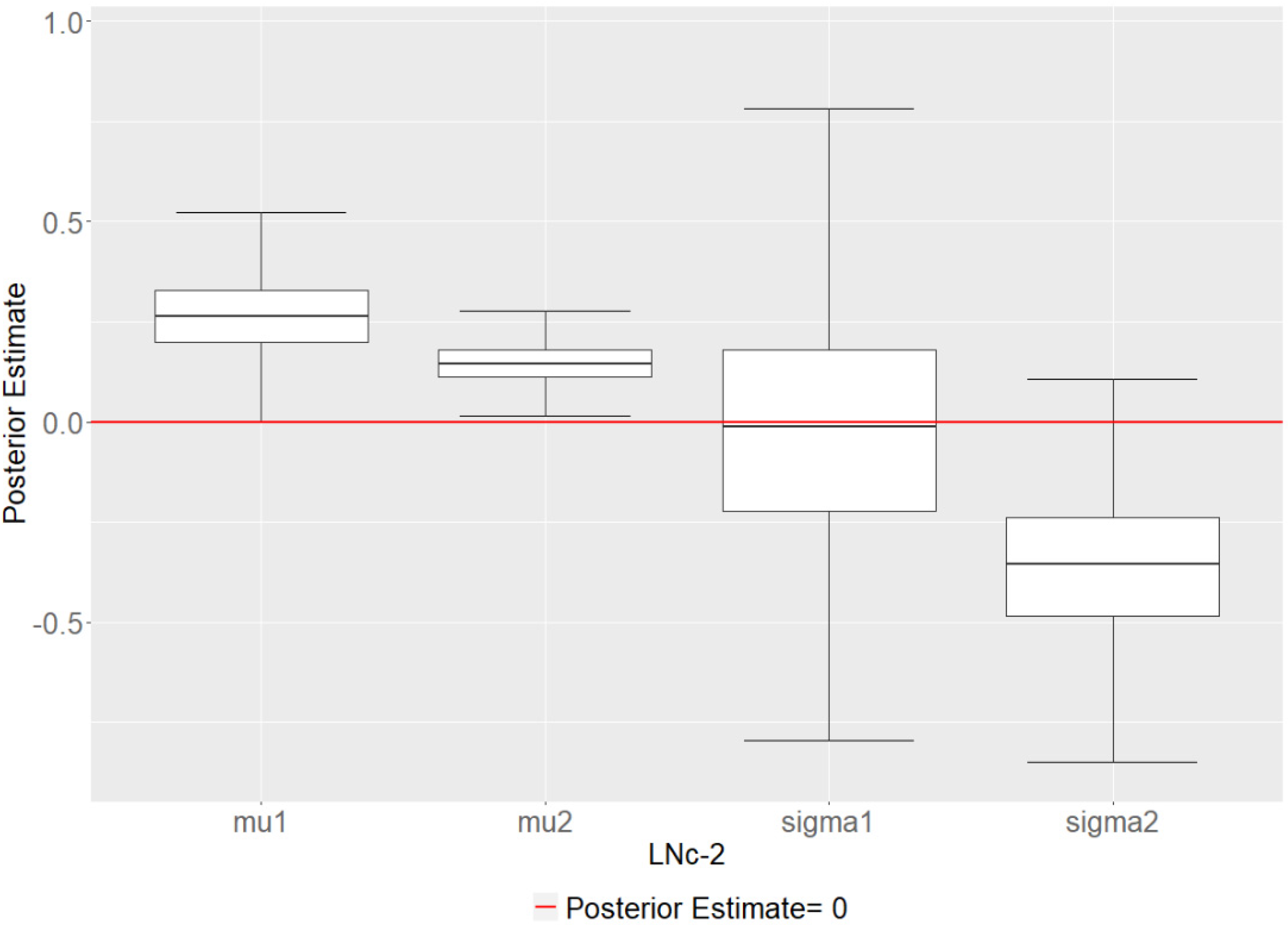
4.2. Variability and Uncertainty of Flood Risk

To distinguish nonstationary patterns in annual extreme flood events of the Xiangjiang River basin, we investigate the detailed linkage between climate variables and flood variability analyzed in Section 2.2. On the basis of the above analysis, the LN_C-3 nonstationary model, with the mean as linear function of JJA AO and SLPa2-PC1 and the log variance as linear function of JJA SLPa2-PC1, is selected as the optimal model among all candidate models. Furthermore, the centile curve is chosen to confirm whether the optimal model explains the physical variation in extreme flood events. The percentages of observation points below the 5th, 25th, 50th, 75th and 95th centile curves are 5.1%, 30.5%, 44.1%, 71.2% and 96.6% in LN_C-3 (Figure 7). The decent coverage rate illustrates that the climate-informed model performs satisfactorily in modeling the variability of the flood observations and their dependence structure over climate variables.

Figure 8 displays the median, 0.95 and 0.99 flood quantiles (i.e., 2-year, 20-year and 100-year events) in the physical-based condition with the LN_C-3 model against the large-scale climate variables JJA AO and SLPa2-PC1, respectively. As seen, the extreme flood risk increases with the climate covariates and the increasing degree with AO is greater than with SLPa2-PC1, which is suggested by the positive variation in mean with bigger coefficient of AO but relatively slight negative in variance on SLPa2-PC1 in LN_C-3 model. It is interesting to note that the flood quantiles evolve with the two important climatic factors with a similar pattern as that between AMFP and two drivers. Consequently, it indicates that the surface atmospheric pressure difference between the northern middle latitude and North Pole compared to the sea level pressure in the Northwest Pacific Ocean have strong teleconnection and influence on extreme flooding of the Xiangjiang River basin. To sum up, if the AO and sea level pressure in the Northwest Pacific Ocean are high, in the same season, the more extreme flooding of the Xiangjiang River will occur during summer. The climate-based optimal nonstationary modeling of results improves the quality of flood quantiles estimation compared to traditional frequency analysis and non-significant time-varying models. The significant inter-relations between the flood risk system and large-scale climate patterns will aid decision makers and scientists to better understand variability in extreme flood risk.

4.3. Return Period and Associated Uncertainty Analysis

The occurrence of extreme flood events is fully estimated by climate-covariates nonstationary frequency analysis. Then, the corresponding return periods are calculated by the appropriate nonstationary design method ENE for at-site flood (details refer to Section 3.5) based on the optimal model LN_C-3. Considering the limited sample size of climatic factors and flood, we investigate the 5-, 10-, 20- and 50-year return periods, which correspond to flood control standards cover most of the major cities in the Xiangjiang River basin and most regions in Changsha, the provincial capital city of Hunan Province. Figure 9 shows the return level differences between conventional stationary model LN_S and time-based nonstationary model LNt-2 compared to climate-based nonstationary model LN_C-3, respectively. Specifically, for LNt-2 and LN_S models, the differences are discernable but within 20% during the 10-year and 50-year return levels, and are minor in recurrence periods shorter than 10-year or longer than 50-year. However, there is a gradually increasing gap from 5-year to 59-year return periods between traditional and nonstationary climate-informed models.

Furthermore, we also explore the change rate (%) in the return periods of AMFP between climate-covariates nonstationary and stationary models, which is given by the following,

$$v=\frac{nrp-srp}{srp}$$

(13)

where $nrp$ and $srp$ are the return periods of the nonstationary and stationary model, respectively. The change rates of 5-, 10-, 20- and 50-year return levels between LN_C-3 and LN_S are 25.2%, 32.2%, 29.1% and 22.6%, respectively, which coincide with the variation trends (i.e., −6.34%, −6.94%, −5.16% and −3.26% respectively) of design flood values in

Table 4. The design flood values comparison between stationary and climate-based nonstationary conditions Unit: m³/s.

Models	5-Year	10-Year	20-Year	50-Year
LNS	16,431	18,806	21,023	23,833
LNC-3	15,356	17,501	19,938	23,056
Variation (%)	−6.34	−6.94	−5.16	−3.26

. Combing with the plot in Figure 9b, it is demonstrated that the occurrence probability of the extreme flood event with nonstationary climate model is obviously smaller than the stationary benchmark. This has great implication for flood control operation and design.

We also compare the statistical characteristics between the models LN_S and LN_C-3. Firstly, based on the fitting results of models LN_S and LN_C-3, the exceedance probabilities of annual extreme flood events during 1959–2017 are investigated. In the comparison of two models, the average exceedance probabilities value of 50.03% for model LN_C-3 is slightly larger than the value of 49.16% for model LN_S, which reveals that the occurrence probabilities of most annual extreme flood events during 1959–2017 have a small increasing trend influenced by climate factors. Secondly, however, on the basis of the expected number of exceedances (ENE) method, the return periods of model LN_C-3 are bigger than the ones for stationary conditions. Thus, based on the design flood values under 5-, 10-, 20-, and 50-year return periods of model LN_C-3 (Table 4), we investigate the exceedance probabilities of each design flood for the corresponding first 5-, 10-, 20-, and 50-years respectively during 1959–2017 (for instance, for the design flood value of 15,356 m³/s over a 5-year return period, we calculate the exceedance probabilities of the ‘15,356 m³/s’ flood event in first 5 years) using models LN_S and LN_C-3. The annual exceedance probabilities differences between the two models are illustrated in Figure 10. As can be seen, for each design flood, all the multi-year average exceedance probabilities of model LN_C-3 are smaller than the stationary model LN_S benchmark.

The above two conclusions are opposite, prompting us to explore the reasons why the annual maximum flood peak series in the Xiangjiang River Basin exhibit different results. Thus, as the parameters of model LN_C-3 are distinct every year from 1959 to 2017, the location and scale parameters for LN_C-3 are averaged, respectively, to investigate the climate-based model’s statistical characteristic in an average sense. In contrast to the model LN_S location parameter of 9.45 and scale parameter of −1.17, the model LN_C-3 average location parameter of 9.453 is slightly larger and the scale parameter of −1.29 is visibly smaller. Furthermore, the probability density distribution curves and exceedance probability distribution curves for two models are demonstrated in Figure 11. The figures clearly introduce that with the extreme flood event values larger than approximately 12,500 m³/s, the average exceedance probabilities of model LN_C-3 are less than the ones in LN_S.

Consequently, from the mathematical point of view, since medium and small extreme flood events are prone to occur, while large flood events are relatively infrequent during the period of 1959–2017, the average exceedance probability for model LN_C-3 is slightly larger than the value of model LN_S. Owing to the 5-year design flood with 15,356 m³/s over 12,500 m³/s, the return periods of model LN_C-3 are generally bigger than the ones under stationary conditions. On the physical aspect being attributed to the two climate factors’ effects, the extreme flood events during the period of 1959–2017 display a mild increasing trend in mean but comparatively descend significantly in variance. In summary, the relatively large decrease in variance contributes to the reduction of exceedance probabilities in model LN_C-3.

Regarding the uncertainty with 50% confidence intervals of nonstationary climate-covariate models for AMFP compared to traditional return levels illustrated in Figure 12, it is remarkably large and fully exceeds the 1:1 line. The phenomenon is highly generated by the ENE method because of its calculative restriction relying on covariate length. Hence, the computation will definitely bring about higher levels of uncertainties [22]. However, the abovementioned results indicate that the occurrence periods of AMFP estimated by a climate-informed model are longer than return periods under a stationary model, which will be conservative for decision makers in considering the significant climatic factors in current conditions. However, since the design floods or return periods rely on the climate covariates, it should not be overlooked that the flood risk would be abnormal if the climatic factors are unusual in future uncommon conditions. Consequently, it is worth noticing that the great uncertainty is a warning for engineers and planners in flood control.

5. Conclusions

The study contributes to describing the characteristics of extreme flood risks under a changing climate, using nonstationary flood frequency analysis models in the Xiangjiang River basin in South-Central China. The paper aims to determine the most significant correlated climatic factors with annual maximum flood peak series, to identify the best model for extreme flood frequency analysis considering different criteria, and to estimate the uncertainties of extreme flood quantiles and return periods based on a Bayesian modeling inference framework. The following main conclusions can be drawn from this study.

(1)

While the stationary frequency analysis is commonly used for hydraulic structure design, recent multiple studies highlighted the increase in the nonstationary pattern of extreme events. In this study, we performed stationary and nonstationary frequency based on the annual maximum flood peak series covering a period of 1959–2017 in the Xiangjiang River basin. Prior to implementing the nonstationary frequency analysis, the selection of physical covariates is an important step. Since most of the extreme floods conventionally occur during the summer season, from June to August, mainly caused by precipitation from the East Asian monsoon, we consider the physical impacts primarily on climatic factors including the eight large-scale low-frequency standard climate indices and two oceanic-atmospheric climate patterns SSTa and SLPa. The identification screening process of potential climate covariates is divided into two steps: the Spearman rank correlation test with AMFP and constructing GLMs to obtain the best combination of climatic impactors. Overall, two distinct climate covariates, which are Arctic Oscillation and the most informative factor, PC1, derived from the SLPa in the Northwest Pacific Ocean during the period of June to August, are identified as the statistically significant positive correlation with AMFP. The abovementioned best processes for screening significant climate drivers can serve as a protocol to apply on other basins.

(2)

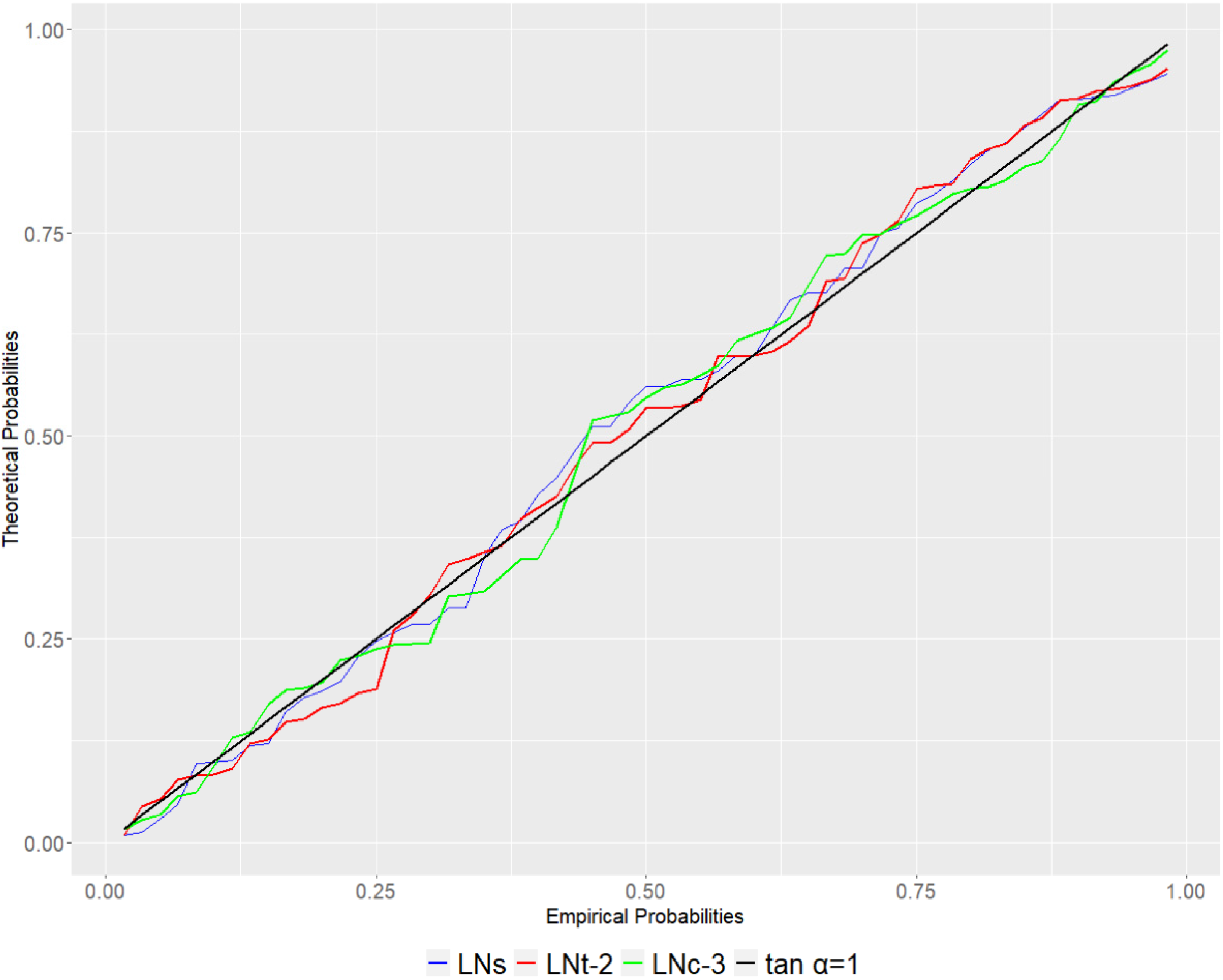
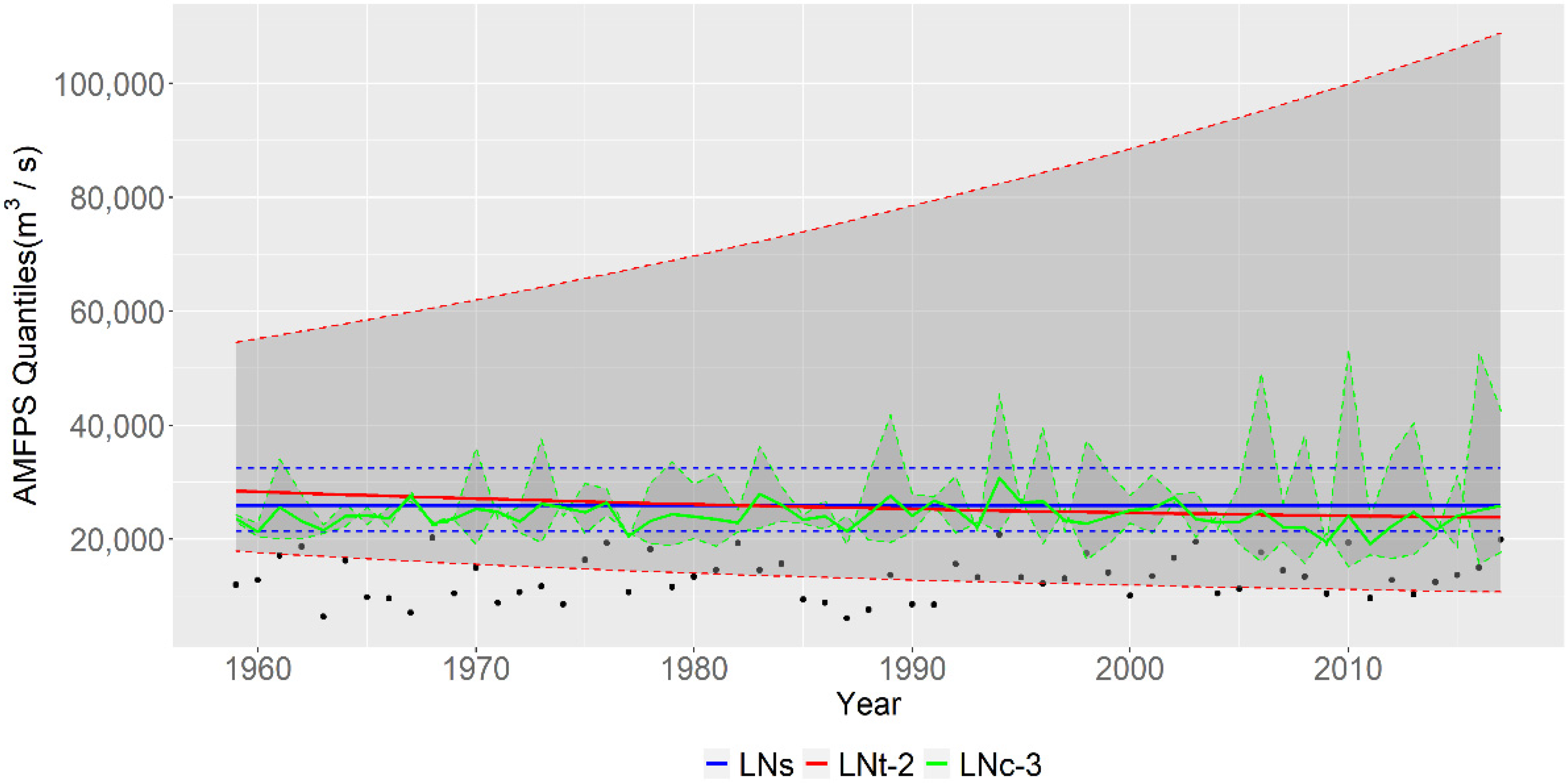
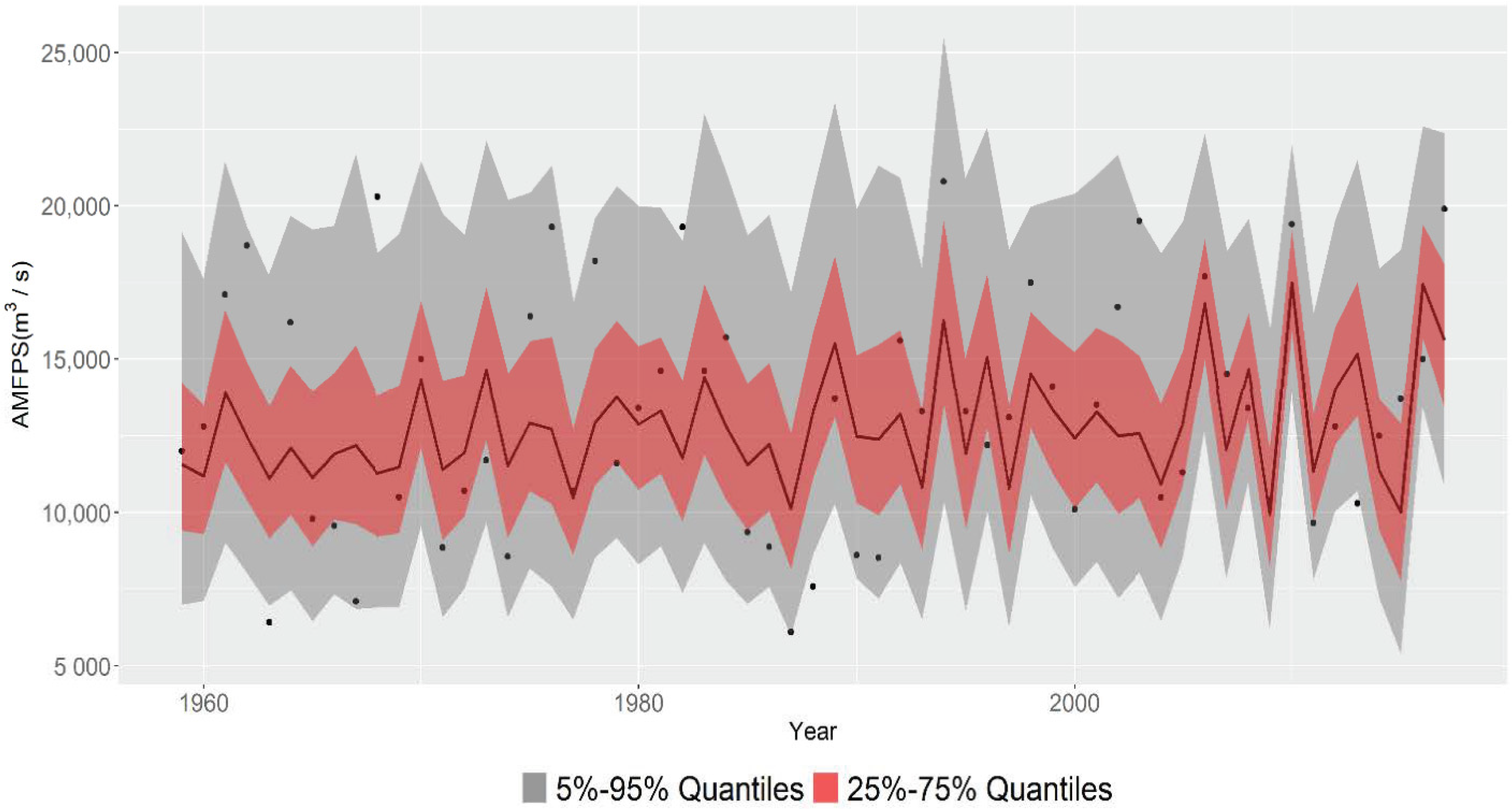
The stationary model and nonstationary flood frequency models with time or climate covariates are evaluated for AMFP employing the two-parameter lognormal distribution, which is an excellent and parsimonious model for representing the distribution of AMFP, and is consistent with the recommendation of other researchers [15]. The results show that extreme flood events follow the nonstationary climate pattern, namely, the optimal model is the nonstationary climate-covariates model with a linearly positive effect on location parameters of two climatic factors and a linearly negative coefficient on scale parameter only for SLPa2-PC1. In addition, the Bayesian modeling inference is used to explore the uncertainty in extreme flood risks. Comparing the three optimal models, namely, LN_S, LNt-2 and LN_C-3 in each case, the time trend in AMFP is so minor that the LNt-2 model parameter coefficients are very close to zero. However, the flood quantiles estimated by the LN_C-3 model, and that used JJA AO and SLPa2-PC1, oscillate over time along with the variation trend of true observed flood. It should be pointed out that the uncertainty boundary of flood quantiles for the LN_C-3 model is relatively high especially for large floods. However, the climate-based model LN_C-3 proved reasonable and improves the understanding and interpretation of changing properties of AMFP frequency, which is apparently influenced by the same season AO and SLPa in the Northwest Pacific Ocean. The linkage between the flood extremes and the climatic factors would be useful to provide reliable and valid information under a changing environment.

(3)

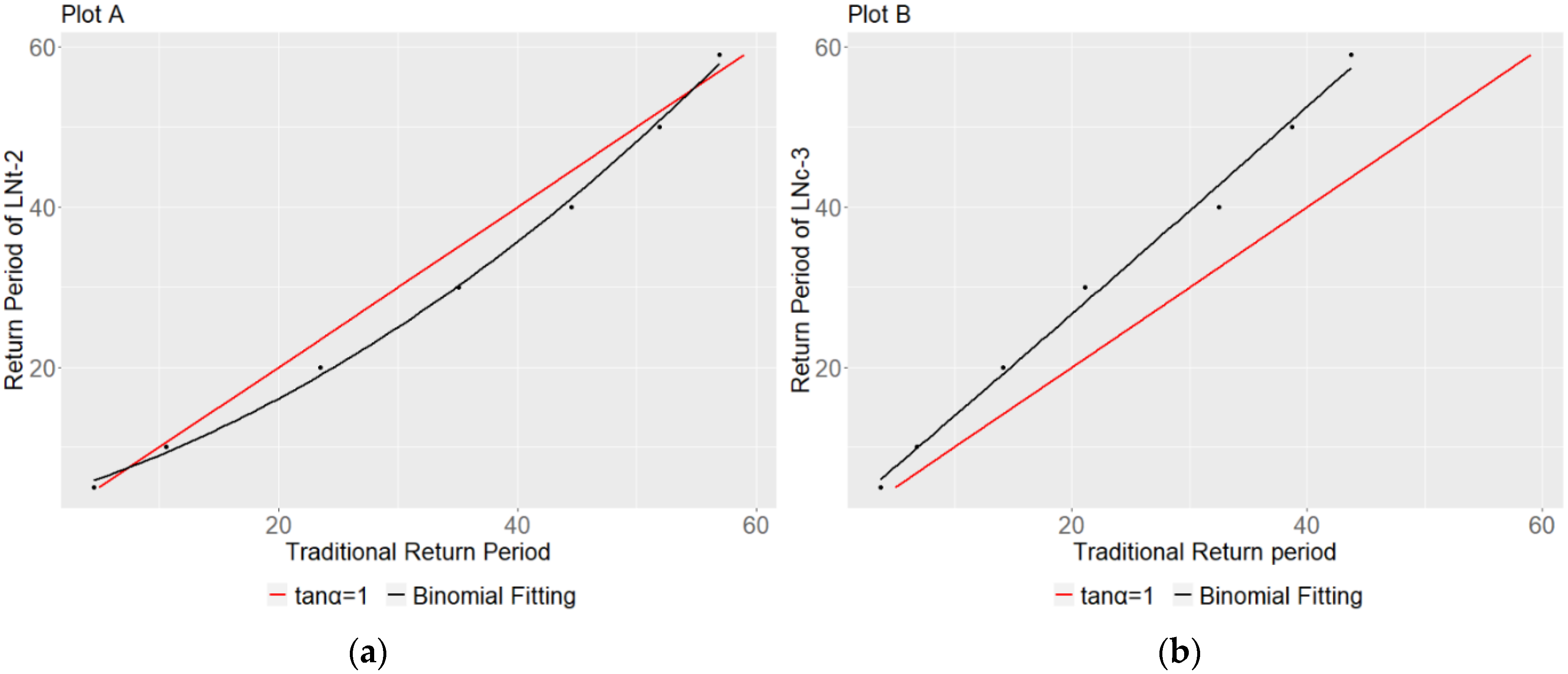
It is interesting to discover that, based on the nonstationary extreme flood analysis, the return periods associated with extreme flood events, computed by the ENE method restricted to the associated timespan of the covariates, are obviously enlarged compared to the stationary approach; the difference is gradually increasing according to the existing trends. In addition, assigning a return period, although the change rates between the LN_S and LN_C-3 model are not registering as high design flood values under current conditions, the larger discrepancies would be found once the climate covariates are located in future uncommon conditions. Nevertheless, the high levels of 50% confidence interval uncertainty boundaries for nonstationary return periods are indeed crossing the 1:1 line in contrast to traditional return levels, which is the major disadvantage of the ENE method. Actually, in order to reduce the uncertainties, the model structures of nonstationary lognormal distribution are set to be simple with a linear trend in distribution parameters. Nevertheless, the uncertainty boundary is still evidently large so that, in the future, new approaches should be pursued to manage or balance the uncertainties of the nonstationary modeling, e.g., by combing more extreme flood events from surrounding stations to collect regional information.

References

1. Zisopoulou, K.; Panagoulia, D. An In-Depth Analysis of Physical Blue and Green Water Scarcity in Agriculture in Terms of Causes and Events and Perceived Amenability to Economic Interpretation. Water 2021, 13, 1693. [Google Scholar] [CrossRef]
2. Panagoulia, D.; Mamassis, N.; Gkiokas, A. Deciphering the Floodplain Inundation Maps in Greece. In Proceedings of the 8th International Conference Water Resources Management in an Interdisciplinary and Changing Context, Porto, Portugal, 26–29 June 2013; pp. 323–330. [Google Scholar]
3. Barichivich, J.; Gloor, E.; Peylin, P.; Brienen, R.J.W.; Schöngart, J.; Espinoza, J.C.; Pattnayak, K.C. Recent intensification of Amazon flooding extremes driven by strengthened Walker circulation. Sci. Adv. 2018, 4, eaat8785. [Google Scholar] [CrossRef] [Green Version]
4. Mangini, W.; Viglione, A.; Hall, J.; Hundecha, Y.; Ceola, S.; Montanari, A.; Rogger, M.; Salinas, J.L.; Borzì, I.; Parajka, J. Detection of trends in magnitude and frequency of flood peaks across Europe. Hydrol. Sci. J. 2018, 63, 493–512. [Google Scholar] [CrossRef] [Green Version]
5. Willner, S.N.; Otto, C.; Levermann, A. Global economic response to river floods. Nat. Clim. Change 2018, 8, 594–598. [Google Scholar] [CrossRef]
6. He, C.; Chen, F.; Long, A.; Luo, C.; Qiao, C. Frequency Analysis of Snowmelt Flood Based on GAMLSS Model in Manas River Basin, China. Water 2021, 13, 2007. [Google Scholar] [CrossRef]
7. López, J.; Francés, F. Non-stationary flood frequency analysis in continental Spanish rivers, using climate and reservoir indices as external covariates. Hydrol. Earth Syst. Sci. 2013, 17, 3189–3203. [Google Scholar] [CrossRef] [Green Version]
8. Ficchì, A.; Cloke, H.; Neves, C.; Woolnough, S.; Coughlan de Perez, E.; Zsoter, E.; Pinto, I.; Meque, A.; Stephens, E. Beyond El Nio: Unsung climate modes drive African floods. Weather Clim. Extrem. 2021, 33, 100345. [Google Scholar] [CrossRef]
9. Zhou, Y. Exploring multidecadal changes in climate and reservoir storage for assessing nonstationarity in flood peaks and risks worldwide by an integrated frequency analysis approach. Water Res. 2020, 185, 116265. [Google Scholar] [CrossRef]
10. Zhang, Q.; Gu, X.; Singh, V.P.; Xiao, M.; Chen, X. Evaluation of flood frequency under non-stationarity resulting from climate indices and reservoir indices in the East River basin, China. J. Hydrol. 2015, 527, 565–575. [Google Scholar] [CrossRef]
11. Kundzewicz, Z.W.; Szwed, M.; Pińskwar, I. Climate Variability and Floods—A global Review. Water 2019, 11, 1399. [Google Scholar] [CrossRef] [Green Version]
12. Kundzewicz, Z.W.; Huang, J.; Pinskwar, I.; Su, B.; Szwed, M.; Jiang, T. Climate variability and floods in China—A review. Earth-Sci. Rev. 2020, 211, 103434. [Google Scholar] [CrossRef]
13. Zeng, H.; Sun, X.; Lall, U.; Feng, P. Nonstationary extreme flood/rainfall frequency analysis informed by large-scale oceanic fields for Xidayang Reservoir in North China. Int. J. Clim. 2017, 37, 3810–3820. [Google Scholar] [CrossRef]
14. Renard, B.; Lall, U. Regional frequency analysis conditioned on large-scale atmospheric or oceanic fields. Water Res. Res. 2014, 50, 9536–9554. [Google Scholar] [CrossRef] [Green Version]
15. Yan, L.; Xiong, L.; Guo, S.; Xu, C.Y.; Xia, J.; Du, T. Comparison of four nonstationary hydrologic design methods for changing environment. J. Hydrol. 2017, 551, 132–150. [Google Scholar] [CrossRef]
16. Olsen, R.; Lambert, J.H.; Haimes, Y.Y. Risk of extreme events under nonstationary conditions. Risk Anal. 1998, 18, 497–510. [Google Scholar] [CrossRef]
17. Salas, J.D.; Obeysekera, J. Revisiting the concepts of return period and risk for nonstationary hydrologic extreme events. J. Hydrol. Eng. 2014, 19, 554–568. [Google Scholar] [CrossRef] [Green Version]
18. Parey, S.; Hoang, T.T.H.; Dacunha Castelle, D. Different ways to compute temperature return levels in the climate change context. Environmetrics 2010, 21, 698–718. [Google Scholar] [CrossRef]
19. Parey, S.; Malek, F.; Laurent, C.; Dacunha-Castelle, D. Trends and climate evolution: Statistical approach for very high temperatures in France. Clim. Change 2007, 81, 331–352. [Google Scholar] [CrossRef] [Green Version]
20. Rootzén, H.; Katz, R.W. Design life level: Quantifying risk in a changing climate. Water Resour. Res. 2013, 49, 5964–5972. [Google Scholar] [CrossRef] [Green Version]
21. Liang, Z.; Hu, Y.; Huang, H.; Wang, J.; Li, B. Study on the estimation of design value under non-stationary environment. South-to-North Water Transf. Water Sci. Technol. 2016, 14, 50–53, (In Chinese with English abstract). [Google Scholar]
22. Yan, L.; Xiong, L.; Luan, Q.; Jiang, C.; Yu, K.; Xu, C.Y. On the Applicability of the Expected Waiting Time Method in Nonstationary Flood Design. Water Resour. Manag. 2020, 34, 2585–2601. [Google Scholar] [CrossRef]
23. Hu, Y.; Liang, Z.; Singh, V.P.; Zhang, X.; Wang, J.; Li, B.; Wang, H. Concept of equivalent reliability for estimating the design flood under non-stationary conditions. Water Resour. Manag. 2018, 32, 997–1011. [Google Scholar] [CrossRef]
24. Gu, X.; Zhang, Q.; Singh, V.P.; Xiao, M.; Cheng, J. Nonstationarity-based evaluation of flood risk in the Pearl River basin: Changing patterns, causes and implications. Hydrol. Sci. J. 2017, 62, 246–258. [Google Scholar] [CrossRef]
25. Mao, D.; Li, J.; Gong, C.; Peng, J. Study on the Flood-Waterlogging Disaster in Hunan Province; Hunan Normal University Press: Changsha, China, 2000. (In Chinese) [Google Scholar]
26. Du, J.; He, F.; Shi, P.J. Integrated flood risk assessment of Xiangjiang River Basin in China. J. Nat. Dis. 2006, 15, 8–44, (In Chinese with English abstract). [Google Scholar]
27. Rayner, N.A.; Parker, D.E.; Horton, E.B.; Folland, C.K.; Alexander, L.V.; Rowell, D.P.; Kent, E.C.; Kaplan, A. Global analyses of sea surface temperature, sea ice, and night marine air temperature since the late nineteenth century. J. Geophys. Res.-Atmos. 2003, 108, 1063–1082. [Google Scholar] [CrossRef]
28. Allan, R.; Ansell, T. A New Globally Complete Monthly Historical Gridded Mean Sea Level Pressure Dataset (HadSLP2): 1850–2004. J. Clim. 2006, 19, 5816–5842. [Google Scholar] [CrossRef] [Green Version]
29. Song, Z.; Xia, J.; She, D.; Zhang, L. The development of a Nonstationary Standardized Precipitation Index using climate covariates: A case study in the middle and lower reaches of Yangtze River Basin, China. J. Hydrol. 2020, 588, 125115. [Google Scholar] [CrossRef]
30. Li, S.; Feng, G.; Wei, H. Summer drought patterns in the middle-lower reaches of the yangtze river basin and their connections with atmospheric circulation before and after 1980. Adv. Meteorol. 2016, 2016, 8126852. [Google Scholar] [CrossRef]
31. Qian, C.; Yu, J.Y.; Chen, G. Decadal summer drought frequency in China: The increasing influence of the Atlantic Multi-decadal Oscillation. Environ. Res. Lett. 2014, 9, 124004. [Google Scholar] [CrossRef] [Green Version]
32. Gong, D.; Zhu, J.; Wang, S. Significant relationship between spring AO and the summer rainfall along the Yangtze River. Chin. Sci. Bull. 2002, 47, 948–952. [Google Scholar] [CrossRef]
33. Wei, F. Relationships between precipitation anomaly over the middle and lower reaches of the Changjiang River in summer and several forcing factors. Chin. J. Atmos. Sci. 2006, 30, 202–211, (In Chinese with English abstract). [Google Scholar]
34. Yang, H. The significant relationship between the Arctic Oscillation (AO) in December and the January climate over South China. Adv. Atmos. Sci. 2011, 28, 398–407. [Google Scholar] [CrossRef]
35. Gong, D.; Wang, S. Influence of Arctic Oscillation on winter climate over China. J. Geogr. Sci. 2003, 13, 208–216. [Google Scholar] [CrossRef]
36. Su, C.; Chen, X. Covariates for nonstationary modeling of extreme precipitation in the Pearl River Basin, China. Atmos. Res. 2019, 229, 224–239. [Google Scholar] [CrossRef]
37. Thompson, D.W.J.; Wallace, J.M. The arctic oscillation signature in the wintertime geopotential height and temperature fields. Geophys. Res. Lett. 1998, 25, 1297–1300. [Google Scholar] [CrossRef] [Green Version]
38. McLeod, A.I.; Xu, C.; Yanhao, L. Package ‘Bestglm’. Available online: http://cran.r-project.org/web/packages/bestglm/bestglm.pdf (accessed on 5 July 2021).
39. Zhao, P.; Zhou, Z. An East Asian subtripical summer monsoon index and its relationship to summer rainfall in China. Acta Meteor. Sin. 2009, 23, 18–28. [Google Scholar]
40. Yunyun, L.; Ping, L.; Ying, S. Basic features of the Asian summer monsoon system. In The Asian Summer Monsoon: Characteristics, Variability, Teleconnections and Projection, Part I; Elsevier: Amsterdam, The Netherlands, 2019; pp. 3–22. [Google Scholar]
41. Vogel, R.M.; Wilson, I. Probability distribution of annual maximum, mean, and minimum streamflows in the United States. J. Hydrol. Eng. 1996, 1, 69–76. [Google Scholar] [CrossRef]
42. Serago, J.M.; Vogel, R.M. Parsimonious Nonstationary Flood Frequency Analysis. Adv. Water Res. 2018, 112, 1–16. [Google Scholar] [CrossRef]
43. Interagency Advisory Committee on Water Data. Guidelines for Determining Flood Flow Frequency: Bulletin 17b (Revised and Corrected); Interagency Committee on Water Data: Washington, DC, USA, 1982; p. 28. [Google Scholar]
44. Aziz, R.; Yucel, I. Assessing nonstationarity impacts for historical and projected extreme precipitation in Turkey. Theor. Appl. Clim. 2021, 143, 1213–1226. [Google Scholar] [CrossRef]
45. Hoffman, M.D.; Gelman, A. The No-U-Turn Sampler: Adaptively Setting Path Lengths in Hamiltonian Monte Carlo. J. Mach. Learn. Res. 2014, 15, 1593–1623. [Google Scholar] [CrossRef]
46. Betancourt, M. A Conceptual Introduction to Hamiltonian Monte Carlo. arXiv 2017, arXiv:1701.02434. Available online: https://arxiv.org/pdf/1701.02434.pdf (accessed on 16 September 2021).
47. Stan Development Team. RStan: The R Interface to Stan, Version 2.21.2. Available online: http://mc-stan.org/rstan.html (accessed on 2 July 2021).
48. Vehtari, A.; Gelman, A.; Gabry, J. Practical Bayesian Model Evaluation Using Leave-One-Out Cross-Validation and WAIC. Stat. Comput. 2017, 27, 1413–1432. [Google Scholar] [CrossRef] [Green Version]
49. Akaike, H. New look at statistical-model identification. IEEE Trans. Autom. Control 1974, 19, 716–723. [Google Scholar] [CrossRef]
50. Schwarz, G. Estimating the dimension of a model. Ann. Stat. 1978, 6, 461–464. [Google Scholar] [CrossRef]
51. Spiegelhalter, D.J.; Linde, A.V.D. Bayesian measures of model complexity and fit. J. R. Stat. Soc. B 2002, 64, 583–616. [Google Scholar] [CrossRef] [Green Version]
52. Li, Y.; Yu, J.; Zeng, T. Deviance Information Criterion for Bayesian Model Selection: Justification and Variation. Econ. Stat. Work. Pap. 2017, 10, 1–25. [Google Scholar] [CrossRef]
53. Cooley, D. Return periods and return levels under climate change. In Extremes in a Changing Climate; AghaKouchak, A., Easterling, D., Hsu, K., Schubert, S., Sorooshian, S., Eds.; Springer: Dordrecht, The Netherlands, 2013; pp. 97–114. [Google Scholar]
54. Lilliefors, H.W. On the Kolmogorov-Smirnov test for normality with mean and variance unknown. J. Am. Stat. Assoc. 1967, 62, 399–402. [Google Scholar] [CrossRef]
Figure 1. The location of Xiangjiang River basin and Xiangtan hydrological station.
Water 14 00066 g001
Figure 2. (a) Rank correlation analysis between AMFP and JFM SSTa (a), JJA SLPa (b). The blue SSTa region and orange SLPa regions have significant negative and positive correlation with AMFP, respectively, at 90% confidence interval (i.e., p < 0.1 ).
Water 14 00066 g002
Figure 3. The scatter plots of AMFP versus JJA AO (a) and JJA SLPa2-PC1 (b) respectively.
Water 14 00066 g003
Figure 4. The boxplot of parameters in LNc-2 model.
Water 14 00066 g004
Figure 5. The PP-plot of the optimal models for each case.
Water 14 00066 g005
Figure 6. The 0.99 quantiles (solid lines) and uncertainty with 90% credibility intervals (areas inside the dashed line) of each model. Black dots are the observed AMFP in each year.
Water 14 00066 g006
Figure 7. The centiles curve plots of the optimal model LNC-3.
Water 14 00066 g007
Figure 8. The median, 0.95 and 0.99, quantiles of AMFP plotted against JJA AO (a) and JJA SLPa2-PC1 (b).
Water 14 00066 g008
Figure 9. The return periods comparison between stationary model LNS and time-based model LNt-2 (a) and climate-based model LNC-3 (b).
Water 14 00066 g009
Figure 10. The annual exceedance probabilities differences of model LN C-3 compared to the model LNS corresponding to each design flood. (a) 5-year design flood; (b) 10-year design flood; (c) 20-year design flood; (d) 50-year design flood.
Water 14 00066 g010aWater 14 00066 g010b
Figure 11. The probability density distribution curves and exceedance probability distribution curves for models LNS (the blue curves) and average LNC-3 (the orange curves). (a) Probability density distribution curve; (b) Exceedance probability distribution curve.
Water 14 00066 g011
Figure 12. The uncertainty with 50% credibility intervals between LNC-3 and LNs models.
Water 14 00066 g012