
Groundwater Radon Precursor Anomalies Identification by EMD-LSTM Model


China Earthquake Networks Center, Beijing 100045, China
*
Author to whom correspondence should be addressed.
Water 2022, 14(1), 69; https://doi.org/10.3390/w14010069
Submission received: 20 November 2021
/
Revised: 24 December 2021
/
Accepted: 26 December 2021
/
Published: 1 January 2022
(This article belongs to the Special Issue Earthquakes and Groundwater)
Abstract
:Groundwater radon concentrations can reflect the changes of crustal stress and strain. Scholars and scientific institutions have also recorded groundwater radon precursor anomalies before earthquakes. Therefore, groundwater radon monitoring is an effective means of predicting seismic activities. However, the variation of radon concentrations within groundwater is not only affected by structural factors, but also by environmental factors, such as air pressure, temperature, and rainfall. This causes difficulty in identifying the possible precursor anomalies. Therefore, the EMD-LSTM model is proposed to identify the radon anomalies. This study investigated the time series data of groundwater radon from well #32 located in Sichuan province. Three models (including the LSTM (Long Short-Term Memory) model with auxiliary data, the EMD-LSTM (Empirical Mode Decomposition Long Short-Term Memory) model with auxiliary data, and the EMD-LSTM model without auxiliary data) were developed in order to predict groundwater radon variations. The results indicated that the prediction accuracy of the EMD-LSTM model was much higher than that of the LSTM model, and the EMD-LSTM model without auxiliary data also can obtain an ideal prediction result. Furthermore, the different durations of seismic activities T (T = ±10, ±30, ±50, and ±100) were also investigated by comparing the identification results. The identification rate of the precursor anomalies was the highest when T = ±30. The EMD-LSTM model identified five possible radon anomalies among the seven selected earthquakes. Taking well #32 as an example, we provided a promising method, that was the EMD-LSTM model, to detect the groundwater radon anomalies. It also suggested that the EMD-LSTM model can be used to identify the possible precursor anomalies within future studies.
1. Introduction
Earthquake forecasting is a worldwide challenging problem, and it has a long history littered with failed attempts [1,2]. However, earthquake precursors are regarded as a key to predict earthquakes. Many scholars and researchers suggest geofluids precursors are one of the most potential and anticipated types [3,4]. Among geofluids anomalies induced by seismic activities, some are significantly detected in hydrogeochemical processes that vary in different scales [5,6,7].
Radon (222Rn) has a half-life of approximately 3.8 days and is continuously occurring within soil or rock fissures in nature; thus, making it suitable for studying geological movement processes that occur from hours to days. Many studies documented that groundwater radon concentrations are sensitive to stress/strain in crustal [8,9]. With the preparation and occurrence of earthquakes, the stress/strain can change the development degree of fractures within rocks as well as the flow of groundwater, leading to changes in radon concentrations [10]). Therefore, groundwater radon monitoring is one of the important means of predicting earthquakes [11].
However, previous studies have shown that radon concentrations in groundwater can be affected by numerous factors. Although the deformation and fracture of rocks can change the radon concentrations in groundwater [12,13], radon concentrations are easily influenced by environmental factors, such as rainfall, air pressure, and temperature. Zafrir et al. [14] and Garavaglia et al. [15] revealed that groundwater temperature and air pressure can influence groundwater radon concentrations. Yan et al. [16] demonstrated that radon concentrations in a hot spring may be changed due to the water temperature. Papachristodoulou et al. [17] reported that the radon diffusion in the soil is affected by water saturation. The variations in radon concentration present nonlinear and complex dynamic characteristics, due to the environmental factors. It is difficult to identify the groundwater radon precursor anomalies; therefore, new methods are needed to detect these anomalies.
Previous researchers have advanced some methods to extract hydrogeologic precursor information by conventional statistical and signal processing methods. For example, Yan et al. [18] used wavelet decomposition to remove barometric and earth tidal responses of groundwater levels; thus, obtaining the precursor anomalies. Furthermore, it is inconvenient to select appropriate wavelet bases within the wavelet transform. Chen et al. [19] used the Hilbert Huang transform (HHT) method to detect the transient anomalous signals in groundwater level data; however, HHT still requires auxiliary data. Pu et al. [20] used the first-order difference, variation rate, and trend rate methods in order to extract the precursor information of groundwater temperature in Southeast Gansu. However, some hydrological anomalies were too small to be detected by these methods.
In recent years, a machine learning approach, the Artificial Neural Network (ANN), has been used to identify radon anomalies within groundwater or soil [21]. Zhang et al. [22] used a decision tree method to identify the radon concentration anomalies in a hot spring; however, this method easily overfits the data. The Long Short-Term Memory neural network (LSTM) is suitable for handling long-term and nonlinear data, due to its unique memory system [23]). Zhang et al. [24] successfully used the LSTM neural network to predict groundwater levels within the Hetao Plain. Cai et al. [25] also used the LSTM neural network to predict groundwater levels, geomagnetism, and gravity precursor data; thus, effectively identifying precursor anomalies. Although the LSTM neural network effectively predicts time series data, this method is still challenging when obtaining ideal results for the strongly nonlinear data. Therefore, the nonlinear and nonstationary data can be decomposed into stationary data using the Empirical Mode Decomposition (EMD) method, then the LSTM neural network can be used to simulate the decomposed signals. Finally, all the simulated results are superimposed to improve the model’s prediction accuracy [26].
Sichuan province is the most active and intensive area of medium and strong earthquakes in China. Well #32 is located in Xichang city within the Sichuan province and has a series of high-quality groundwater radon data. Well #32 provided suitable conditions for the identification of radon anomalies by the EMD-LSTM model.
In this paper, we applied the EMD-LSTM method to identify the possible radon anomalies in well #32 from 1 February 2010 to 31 December 2020. This model is suitable for predicting the non-linear and non-stationary data. The main process of this paper is: (1) process the data and supplement the missing data; (2) select the earthquake that may cause the change of radon concentrations in well #32; (3) the data are divided into two parts, one part is the data during seismic activities period, and the other part is the data during non-seismic activities period; (4) establish the EMD-LSTM model, and the data during non-seismic activities period are used as the training set and validation set, then the data during seismic activities period are used as the prediction set; (5) compare the correlation coefficient R2 value between the prediction and the observation values during the period of non-seismic activities (validation set) and the period of seismic activities (prediction set). The difference of correlation coefficient R2 is used as the basis to identify earthquake precursors.
2. Geological Setting
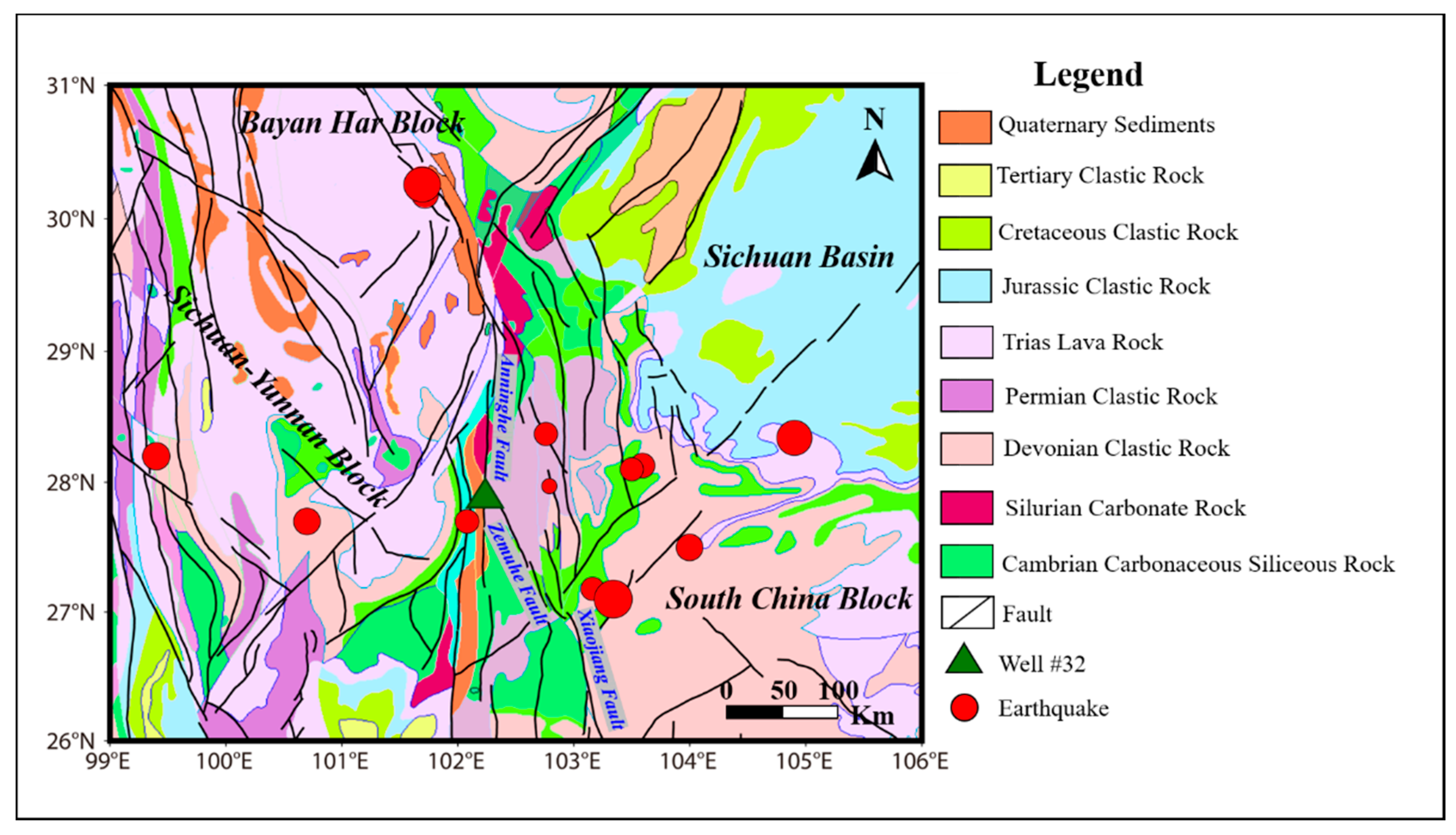
The study area is located on the eastern edge of the Tibet Plateau and is the junction of the Qinghai-Tibet and the Yunnan-Guizhou plateaus. This area is controlled by three strike-slip faults, which are Anninghe fault, Zemuhe fault, and Xiaojiang fault. The Anninghe fault is N-S trending, with a length of approximately 200 km and the Zemuhe fault is NNW-SSE trending, with a length of approximately 120 km. The Zemuhe fault is the connection zone of the Anninghe fault and Xiaojiang fault (Figure 1). Crustal structure can be partitioned into four geological units in this study area: the Sichuan-Yunnan Block of the west, the Bayan Har Block of the north, the South China Block of the southeast, and the Sichuan Basin of the northeast [27,28].
The drilling depth of well #32 is 390 m, and it flows well with confined aquifer. The lithology of observation aquifer (the depth is 259 m to 321 m) is sandstone and mudstone, and it is typical confined fissure water of a deep bedrock structure. The study area is one of the most active and intense areas containing moderate to strong earthquakes. The historical record has shown at least nine strong earthquakes of M ≥ 7 in the past 1200 years within this region [29].
3. Methods and Model
3.1. Data Processing and Seismic Setting
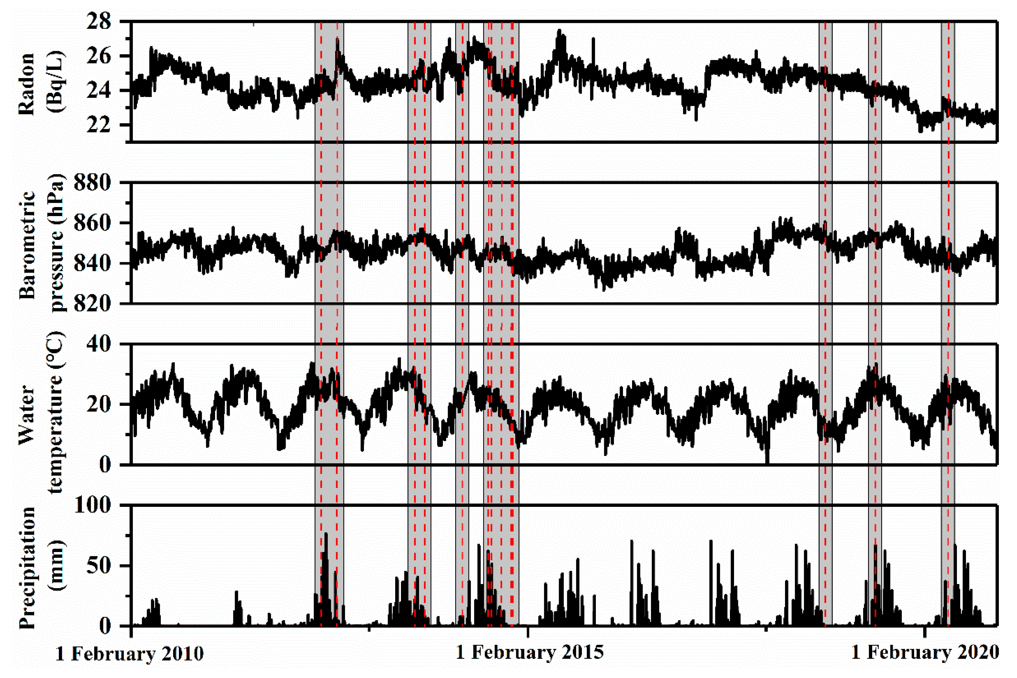
The average daily data of the groundwater radon, air pressure, temperature, and rainfall of well #32 were collected from 1 February 2010 to 31 December 2020. During the monitoring period, the data were only missing for a few days, and the difference method was used to supplement the missing data. However, the air pressure, temperature, and rainfall data were missing from March 19 to December 31 in 2017. The average values of the same two days in 2018 and 2019 were used to supplement the missing data during the same period.
In the process of radon anomalies identification, it is crucial to select the corresponding earthquake. Dobrovolsky [30] proposed a way to determine the precursory anomalies areas according to the earthquake magnitude:
where is the greatest distance that the precursor may appear, is the magnitude, and = 10−8 is the limit for distinguishing between an earthquake preparatory strain and the daily strain loading by earth loads.
In addition, these earthquakes occurred within 3 months and were regarded as one earthquake in order to distinguish the possible precursor and post-seismic effects of consistent earthquakes [22]. Simultaneously, the seismic energy density e (J/m3) was used to verify whether these earthquakes could change the hydrological changes. According to the published global hydrogeology phenomenon after earthquakes, the co-seismic response hydrological changes normally occurred when the seismic energy density was greater than 10−4 (J/m3) [31]. The calculation equation is as follows:
where r is the epicentral distance and e is the seismic energy density.
According to Equations (1) and (2), seven groups of earthquake events were selected (Table 1). Thirty days before and after each group of earthquakes (i.e., T = ±30) was also regarded as the seismic activities period, and the rest of the time was regarded as the non-seismic activities period (Figure 2), as it had the highest identification rate when the duration of seismic activity T = ±30.
3.2. Empirical Mode Decomposition (EMD)
Huang et al. [32] proposed the Empirical Mode Decomposition (EMD) method. EMD is based on direct energy extraction associated with various intrinsic timescales, and can decompose the non-stationary and the non-linear data sets into many intrinsic mode functions (IMFs).
EMD assumes that any signal could contain IMFs, and the IMFs are defined as: (1) the number of zero points that are equal to or have at most one difference from the number of extreme points within the data set; (2) at any point on the signal, the mean value between the upper envelope determined by the maximum point and the lower envelope determined by the minimum point is 0. Therefore, the signal is locally symmetrical about the time axis.
The process of EMD for the data set Xt is:
- (1)
- The maximum and minimum values of the data set are obtained, and the interpolation function is fitted to all extreme points to obtain the upper envelope Ut and the lower envelope Lt.
- (2)
- The average values between the upper and lower envelopes are calculated using the equation:
- (3)
- Let . If the is the IMF, then is equal to . Otherwise, as a new input, repeating the above steps until the IMF is obtained.
- (4)
- Let residual , then as a new input, repeating the steps (1) and (2). When the last residual satisfies monotonicity, the termination conditions are obtained. The original signal Xt can be reconstructed by a series of IMFs and Rt, that is, (Rt is the residual function).
3.3. Long Short-Term Memory (LSTM)
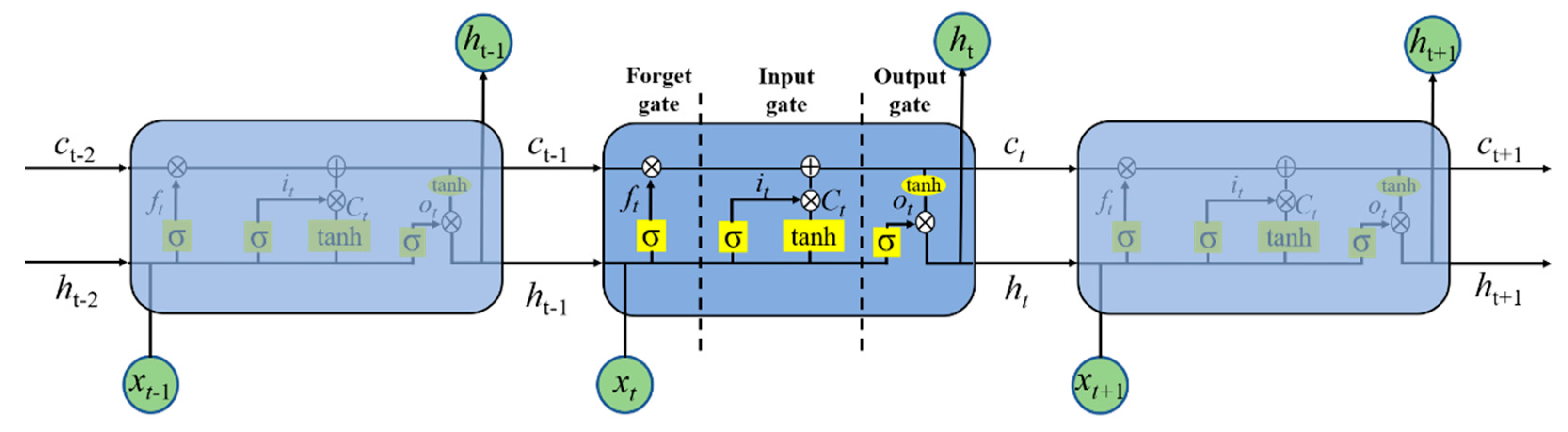
Hochreiter and Schmidhuber [33] first proposed the Long Short-term Memory neural network (LSTM). LSTM is a unique type of Recurrent Neural Network (RNN), and uses gate units and memory cells to effectively overcome the inherent problems of the traditional RNN, such as gradient vanishing and exploding [34,35]. The special structure of the LSTM neural network can effectively deal with long-time scale nonlinear time series data.
The LSTM neural network includes the input layer, hidden layer, and output layer. The hidden layer, that is the LSTM layer, is a special neuron structure designed using three gate units (including the input gate, forget gate, and output gate) and memory cells (Figure 3). , , represent the forget gate, input gate, and output gate, respectively. The unit state runs through the gate structure. In Figure 3, in addition to h flowing over time, unit state c also flows over time.
The forget gate determines which information should be ignored, and is determined by the previous output vector ht−1 and the input vector xt at the current time. The forget gate is defined as:
where is the sigmoid activation function and the output value ranges from 0 to 1 (0 represents that all the information is removed, while 1 represents that it is all retained). W and U are the weight matrices. b is the bias vector. W, U, and b are determined by the training data.
The input gate consists of sigmoid layer and tanh layer. The sigmoid layer determines which information should be updated, and is determined by the tanh layer. Then, the units state ct is updated by .
where is the tanh activation function and is the Hadamard product.
Finally, the output gate controls what information should be output. The output ht is determined by the output gate and the units state ct.
3.4. EMD-LSTM Model Development
According to previous studies, the EMD method has the advantage in signal decomposition, while the LSTM neural network method has the advantage in predicting the long-time series data. Therefore, the EMD-LSTM method presents significant advantages in predicting nonlinear and non-stationary series data sets. To identify radon anomalies, the EMD-LSTM model was developed as:
- (1)
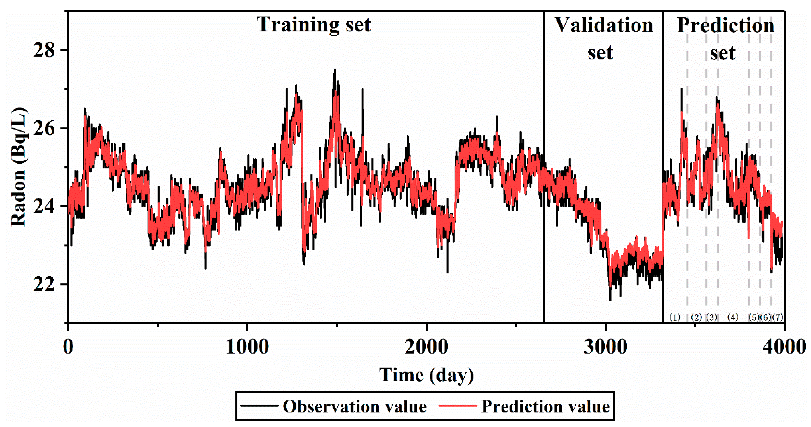
- Collated the data set. The data set (including groundwater radon, air pressure, temperature, and precipitation) during the non-seismic activities period was arranged chronologically. The collated data were then set as training set and validation sets. Next, the data set during the seismic activities period was set as the prediction set. The radon data set after collating is shown in Figure 4.
- (2)
- The EMD method was applied to the collated data set, then the IMFs functions and residual functions Rt were obtained.
- (3)
- The IMFs and Rt were predicted by the LSTM neural network. Eighty percent of the decomposed signal during the period without any earthquakes was set as the training set, and 20% of the decomposed signal during the period without earthquakes was set as the validation set. Then, the 7 seismic activity periods were set as the prediction set.
- (4)
- The EMD decomposition signal’s prediction results were superimposed to obtain the final prediction results.
The hyperparameters of the LSTM neural network (including the number of hidden layers, the number of neurons, and the learning rate) were determined using the control variable method. In this paper, the number of hidden layers was set as 1 layer, and the learning rate was adjusted 3 times. The number of neurons within the hidden layer was determined using the empirical Equation [36]:
where is the number of neurons in the hidden layer, is the number of neurons in the input layer, is the number of neurons in the output layer, and is an integer between 1 and 10.
According to Equation (9), the number of hidden neuron layers was 4–10, and the learning rate was set as {0.0001, 0.0003, 0.001, 0.003, 0.01}. When the hyperparameter was 6 and was 0.0001, the root mean square error (RMSE) was the smallest, and the correlation coefficient (R2) was the largest within the validation set.
In this paper, the loss function loss (LOSS) in the LSTM neural network is defined as follows:
where is the observation value, is the prediction value, and is the number of samples.
The Adam optimization function, which had the characteristics of fast convergence, was used [37]. For efficient learning, the min-max normalization approach was used to scale the range of input variables to (0, 1) before the training process:
where , , , and are the observation, normalized, maximum, and minimum data, respectively. Finally, the inverse normalization was used to obtain the final predicted results.
3.5. Model Performance Criteria
In order to evaluate the prediction results of the EMD-LSTM model, two conventional metrics were adopted in this paper, including the root mean square error (RMSE) and the correlation coefficient (R2). The equations are defined as follows:
where is the observation value, is the prediction value, is the average values of the observation value, and is the number of samples. RMSE is used to measure the degree of the standard deviation between the prediction and the observation values. The smaller the RMSE value, the closer the prediction values are to the observation values. The value of R2 reflects the linear correlation between the prediction and the observation values, and its value range between 0 and 1 (0 indicates no fit, and 1 indicates a perfect fit).
4. Results
4.1. The Result of EMD-LSTM Model Prediction
The prediction results of each decomposition function (including IMFs and Res) by the LSTM neural network were shown in Figure 5. The prediction accuracy of IMF1 to IMF4 was relatively low because the data of IMF1 to IMF4 presented the characteristics of strong nonlinearity. The high-frequency fluctuation signal (IMF1 to IMF4) contained a large number of irregular noises. However, the predicted results of IMF5 to IMF9 and Res were consistent with the observation values. The predicted results can reflect the medium and long-term trends within the time series data.
The prediction results of all decomposed functions were superimposed in order to obtain the final prediction result of the EMD-LSTM model. The prediction results of the training set, validation set, and prediction set are shown in Figure 6. The RMSE value was 0.264 and the R2 value was 0.895 within the training set; in addition, the RMSE value was 0.295 and the R2 value was 0.949 within the validation set. The results indicated that the EMD-LSTM model could effectively predict the time series data of the groundwater radon.
4.2. The Result of Seismic Anomaly Identification
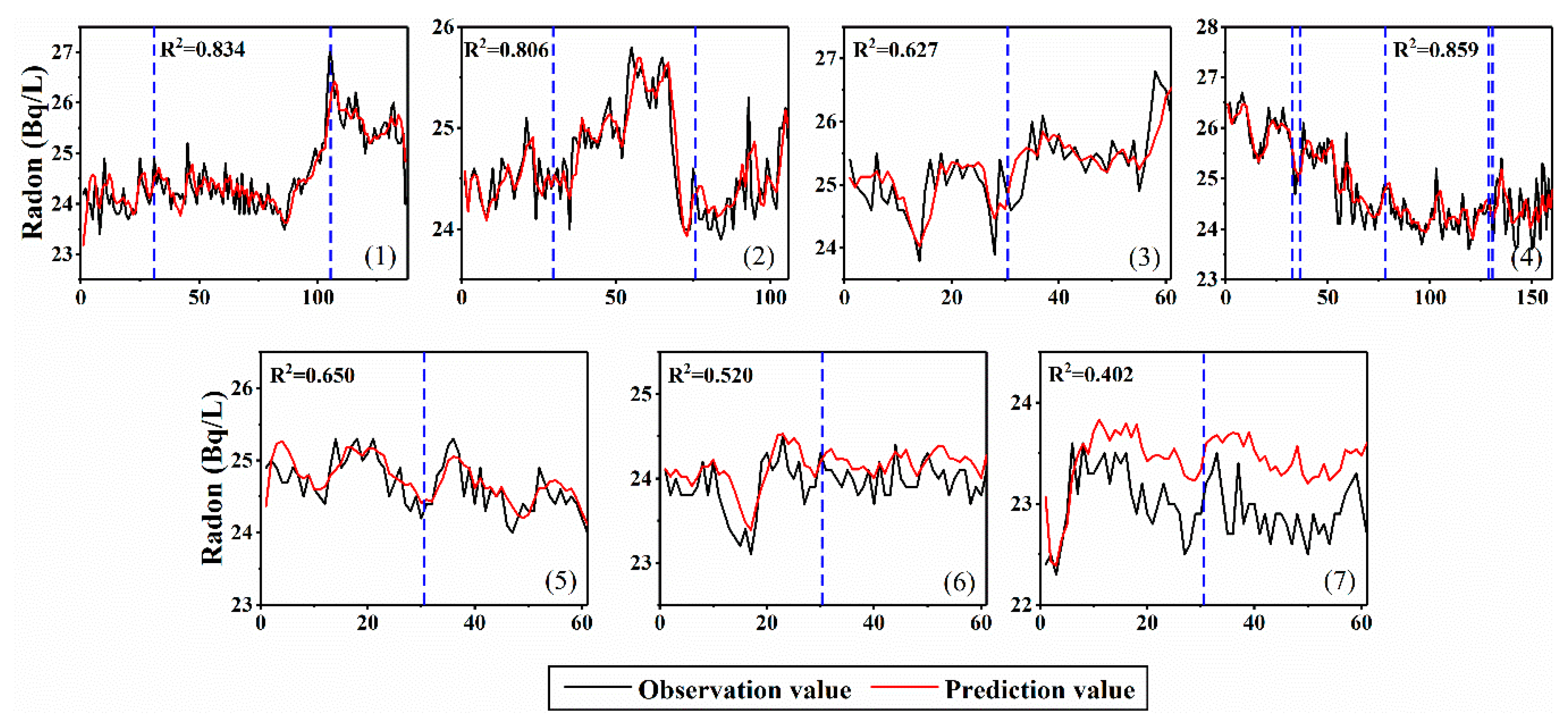
In order to identify the radon anomalies caused by earthquakes, the R2 value between the prediction and the observation values during the period of non-seismic activities (validation set) and the period of seismic activities (prediction set) were compared. If the R2 value during the period of seismic activities was lower than that during the period without earthquakes, it indicated that the earthquake may affect the radon concentrations. The R2 values between the prediction and the observation values during the seismic activity period were shown in Figure 7. The R2 value in the training set was less than the R2 value (R2 = 0.949) in the validation set, especially the R2 value during seismic activity events (3), (5), (6), and (7), their R2 values were 0.627, 0.650, 0.520, and 0.402, respectively.
The radon anomalies can be identified when the differences in the R2 values during non-seismic and seismic activities are greater than 15%. The differences in the R2 values of seven seismic activity events were 12.1%, 15.0%, 33.9%, 9.5%, 31.5%, 44.3%, and 57.6%, respectively. Therefore, the EMD-LSTM model effectively identified five seismic activity events. The results indicated that the EMD-LSTM model was suitable for the anomalies detection.
In order to evaluate the grade of reliability of data analysis approach, we compared this with other research results. Zhang et al. [22] used a decision tree method to identify the groundwater radon anomalies in a hot spring from 1980 to 2008. They identify 15 possible radon anomalies among the 24 chosen earthquakes. In addition, Zhao et al. [28] applied the residual signal processing technique, the Hurst exponent estimates, and statistical standard (the mean ± two standard deviation) to analyze the radon anomalies in well #32 from 1 January 2008 to 31 December 2018. They detected 12 radon anomalies within 20 chosen earthquakes. From the result, the groundwater radon anomalies identification rate by EMD-LSTM method is higher than that by other two methods.
5. Discussion
5.1. Duration of Seismic Activity Impact on Precursor Anomaly Identification
In order to evaluate the impact of complete earthquake events (including earthquake preparation, occurrence, and aftershock) on radon concentrations in groundwater, the identification results of four different seismic activity periods T (i.e., T days before and after the earthquake) were calculated. For example, T = ±10 represented the seismic activity period, which included 10 days before and 10 days after the earthquake. The average R2 value within the non-seismic activity periods (training set and validation set), as well as the average R2 value of the seismic activity period (prediction set) were shown in Table 2.
Although the difference between the validation set and the prediction set was the largest when T = ±10, it has the highest identification rate when T = ±10 and ±30. In order to avoid mixing the radon data that were affected by the seismic activities in the training data, T = ±30 was selected as the duration for the seismic activities within this paper.
5.2. Comparison with Other Models
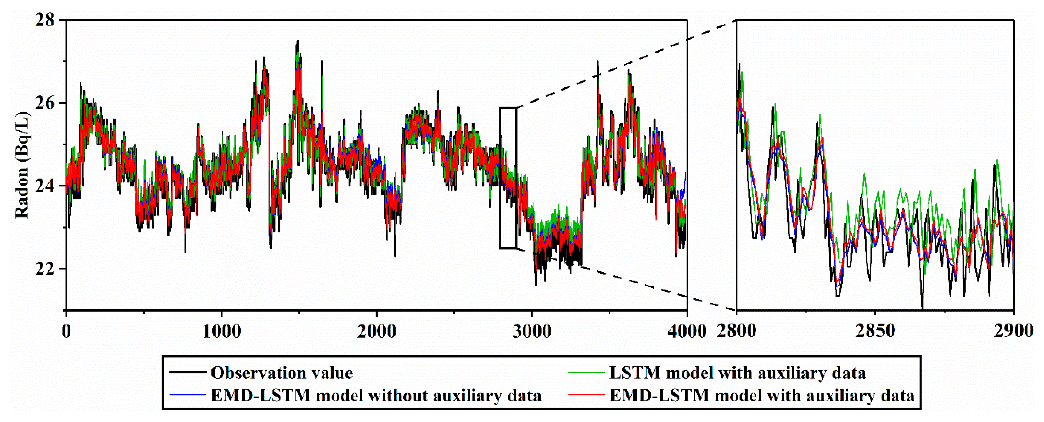
To evaluate the prediction accuracy of EMD-LSTM model, the model’s prediction results of the EMD-LSTM model with auxiliary data (including air pressure, temperature, and precipitation), the EMD-LSTM model without auxiliary data, and the LSTM model with auxiliary data were compared in this study (Figure 8). The R2 value and the RMSE value of the EMD-LSTM model with auxiliary data within the validation set were 0.949 and 0.295, respectively, while the R2 value and the RMSE value of the LSTM model within the validation set were 0.891 and 0.445, respectively. The different results indicated that the prediction accuracy of the EMD-LSTM model was better than that of the LSTM model. In addition, the prediction value of the LSTM model had hysteresis on the observation value. The results indicated that the LSTM model may not be perfect for the strong nonlinear and nonstationary data.
The R2 and the RMSE values of the EMD-LSTM model within the validation set without auxiliary data were 0.949 and 0.273, respectively. It demonstrated that the EMD-LSTM model still had good predicted results when only groundwater radon was used as the input data.
5.3. Mechanism in the Precursory Anomalies of Radon
Although groundwater radon precursor anomalies can be effectively identified using the EMD-LSTM model, the anomalies’ mechanism still needs to be investigated. The variation of the groundwater radon concentrations can be affected by the crustal stress and strain because radon within the rock fissures can be dissolved into the groundwater or volatilized from the groundwater to the fissures.
For example, seismic activity events (2) and (3) showed positive anomalies; that is, the radon concentrations increased before the earthquake. Mollo et al. [38] found that the radon emission rate increased within the rock after the cracks formed, leading to more radon being dissolved in the groundwater. Therefore, the formation of cracks within the rock mass and aquifer system played an important role in increasing the groundwater radon concentration.
As shown in Figure 7, seismic activity events (5)–(7) showed significant negative anomalies; that is, the radon concentration decreased before the earthquakes. The radon concentration can be affected by numerous factors, such as the characteristics of the earthquake fault and the hydrogeological setting. These factors caused different anomaly characteristics. When the radon concentration decreased before the earthquake, the volatilization model can be used to explain this mechanism. It was hypothesized that the rate of the rock masses dilation was faster than that of the groundwater flow into the newly formed cracks; therefore, the radon volatilized from the groundwater to the fissures [39]. Well #32 was located at the junction of the Zemuhe fault and Anninghe fault; therefore, this unique geological structure created favorable conditions for the volatilization model.
There were two contrasting radon anomaly types in same region and same geological condition. This phenomenon still needed to be explained. The same phenomenon also occurred in other observation wells. For example, Panjin observation well has recorded positive anomalies before the Xiuyan Mw 5.1 earthquake and negative anomalies before the Tohoku M 9.1 earthquake. Shao et al. [40] showed that the study area was in a state of compression before the Tohoku M 9.1 earthquake and in a state of tension afterward. It indicated that the endogenous factors that influence radon concentrations are primarily related to stress state [41] (Zhou et al. 2020). In this study, the change in stress state may be the main reason for the different anomalies.
Although the EMD-LSTM model can effectively identify most anomalies, the seismic activity events (1) and (4) still could not be detected. The occurrence of these precursors was primarily related to factors, such as epicentral distance, earthquake magnitude, and duration of the seismic activity [42]. These factors may be the main reasons for the disappearance of the anomalies.
6. Conclusions
Radon concentrations within groundwater or soil reflected the changes in crustal stress and strain levels, providing an effective method in predicting seismic activities. However, radon concentrations in groundwater were easily affected by some environmental factors. Therefore, it was challenging to identify the precursor anomalies. Based on the groundwater radon data of well #32, the precursor anomalies were identified by the EMD-LSTM model in this study. The results indicated: (1) the EMD-LSTM model efficiently identified the possible precursor anomalies. Compared with the LSTM model, the EMD-LSTM model can improve the prediction accuracy and eliminate the prediction hysteresis phenomenon of the LSTM model; (2) the prediction accuracy of the EMD-LSTM model during seismic activities had a significant deviation compared with the results during non-seismic activities; (3) the EMD-LSTM model effectively identified five possible radon anomalies among the seven selected seismic activity events. The results showed that the EMD-LSTM model was a feasible method in the identification of groundwater radon precursor anomalies.
Author Contributions
Conceptualization, X.F. and J.Z. (Jun Zhong); methodology, X.F.; software, X.F.; validation, J.Z. (Jun Zhong), Z.Z. and R.Y.; formal analysis, X.F.; investigation, X.F and L.T.; resources, J.Z. (Jing Zhao); data curation, Z.Y.; writing—original draft preparation, X.F.; writing—review and editing, X.F.; visualization, X.F.; supervision, J.Z (Jun Zhong), Z.Z., L.T. and R.Y.; project administration, J.Z. (Jing Zhao) and Z.Y.; funding acquisition, J.Z. (Jing Zhao). and Z.Y. All authors have read and agreed to the published version of the manuscript.
Funding
This research was financially supported by the National Key R&D Program of China [grant numbers 2018YFE0109700 and 2018YFC150330505], the Natural Science Foundation of China [grant number 11672258], and the Youth Science and Technology Fund of China earthquake Networks Center [grant number QNJJ-202108].
Data Availability Statement
All data during the study are available from the corresponding author by request.
Acknowledgments
We thank two reviewers for constructive for comments and suggestions.
Conflicts of Interest
The authors declare no conflict of interest.
References
- Yan, X.; Shi, Z.; Wang, G.; Zhang, H.; Bi, E. Detection Of Possible Hydrological Precursor Anomalies Using Long Short-Term Memory: A Case Study of the 1996 Lijiang Earthquake. J. Hydrol. 2021, 599, 126369. [Google Scholar] [CrossRef]
- Pritchard, M.; Allen, R.; Becker, T.; Behn, M.; Brodsky, E.; Bürgmann, R.; Ebinger, C.; Freymueller, J.; Gerstenberger, M.; Haines, B.; et al. New Opportunities to Study Earthquake Precursors. Seismol. Res. Lett. 2020, 91, 2444–2447. [Google Scholar] [CrossRef]
- Wang, C.; Manga, M. Groundwater and Stream Composition. In Water and Earthquakes. Lecture Notes in Earth System Sciences; Springer: Berlin/Heidelberg, Germany, 2021. [Google Scholar]
- Moralessimfors, N.; Wyss, R.; Bundschuh, J. Recent progress in radon-based monitoring as seismic and volcanic precursor: A critical review. Crit. Rev. Environ. Sci. Technol. 2020, 50, 979–1012. [Google Scholar] [CrossRef]
- Binda, G.; Pozzi, A.; Michetti, A.M.; Noble, P.J.; Rosen, M.R. Towards the understanding of hydrogeochemical seismic responses in karst aquifers: A retrospective meta-analysis focused on the Apennines (Italy). Minerals 2020, 10, 1058. [Google Scholar] [CrossRef]
- Claesson, L.; Skelton, A.; Graham, C.; Dietl, C.; Mörth, M.; Torssander, P.; Kockum, I. Hydrogeochemical changes before and after a major earthquake. Geology 2004, 68, A247. [Google Scholar] [CrossRef]
- Tsunogai, U.; Wakita, H. Precursory Chemical-Changes In-Ground Water-Kobe Earthquake, Japan. Science 1995, 269, 61–63. [Google Scholar] [CrossRef]
- Riggio, A.; Santulin, M. Earthquake forecasting: A review of radon as seismic precursor. Boll. Geofis. Teor. Appl. 2015, 56, 95–114. [Google Scholar]
- Igarashi, G.; Saeki, S.; Takahata, N.; Sumikawa, K.; Tasaka, S.; Sasaki, Y.; Takahashi, M.; Sano, Y. Groundwater Radon Anomaly Before the Kobe Earthquake in Japan. Science 1995, 269, 60–61. [Google Scholar] [CrossRef]
- Woith, H. Radon earthquake precursor: A short review. Eur. Phys. J. Spec. Top. 2015, 224, 611–627. [Google Scholar] [CrossRef]
- Martinelli, G. Previous, Current, and Future Trends in Research into Earthquake Precursors in Geofluids. Geosciences 2020, 10, 189. [Google Scholar] [CrossRef]
- Nicolas, A.; Girault, F.; Schubnel, A.; Pili, E.; Passelegue, F.; Fortin, J.; Deldicque, D. Radon emanation from brittle fracturing in granites under upper crustal conditions. Geophys. Res. Lett. 2014, 41, 5436–5443. [Google Scholar] [CrossRef]
- Koike, K.; Yoshinaga, T.; Suetsugu, K.; Kashiwaya, K.; Asaue, H. Controls on radon emission from granite as evidenced by compression testing to failure. Geophys. J. Int. 2015, 203, 428–436. [Google Scholar] [CrossRef]
- Zafrir, H.; Barbosa, S.M.; Malik, U. Differentiation between the effect of temperature and pressure on radon within the subsurface geological media. Radiat. Meas. 2013, 49, 39–56. [Google Scholar] [CrossRef]
- Garavaglia, M.; Moro, G.D.; Zadro, M. Radon and tilt measurements in a seismic area: Temperature effects. Phys. Chem. Earth Part A Solid Earth Geod. 2000, 25, 233–237. [Google Scholar] [CrossRef]
- Yan, R.; Woith, H.; Wang, R.; Wang, G. Decadal radon cycles in a hot spring. Sci. Rep. 2017, 7, 12120. [Google Scholar] [CrossRef] [PubMed] [Green Version]
- Papachristodoulou, C.; Ioannides, K.; Spathis, S. The Effect of Moisture Content on Radon Diffusion through Soil: Assessment in Laboratory and Field Experiments. Health Phys. 2007, 92, 257–264. [Google Scholar] [CrossRef]
- Yan, R.; Huang, F.; Chen, Y. Application of Wavelet Decomposition to Remove Barometric and Tidal Response in Borehole Water Level. Earthq. Res. China 2007, 23, 204–210, (In Chinese with English Abstract). [Google Scholar]
- Chen, C.; Wang, C.; Liu, J.; Liu, C.; Liang, W.; Yen, H.; Yeh, Y.; Chia, Y.; Wang, Y. Identification of earthquake signals from groundwater level records using the HHT method. Geophys. J. Int. 2010, 180, 1231–1241. [Google Scholar] [CrossRef] [Green Version]
- Pu, X.; Mei, D.; Chen, Y.; Ye, Y.; Wang, J.; Xu, K. Characteristics analysis on the abnormal changes of the water temperature before and after the Wenchuan Ms8.0 from 4 wells located in southeast of Gansu. Recent Dev. World Seismol. 2014, 2, 17–23, (In Chinese with English Abstract). [Google Scholar]
- Torkar, D.; Zmazek, B.; Vaupoti, J.; Kobal, I. Application of artificial neural networks in simulating radon levels in soil gas. Chem. Geol. 2010, 270, 1–8. [Google Scholar] [CrossRef]
- Zhang, S.; Shi, Z.; Wang, G.; Yan, R.; Zhang, Z. Groundwater radon precursor anomalies identification by decision tree method. Appl. Geochem. 2020, 121, 104696. [Google Scholar] [CrossRef]
- Liu, F.; Cai, M.; Wang, L.; Lu, Y. An Ensemble Model Based on Adaptive Noise Reducer and Over-Fitting Prevention LSTM for Multivariate Time Series Forecasting. IEEE Access 2019, 7, 26102–26115. [Google Scholar] [CrossRef]
- Zhang, J.; Zhu, Y.; Zhang, X.; Ye, M.; Yang, J. Developing a Long Short-Term Memory (LSTM) based model for predicting water table depth in agricultural areas. J. Hydrol. 2018, 561, 918–929. [Google Scholar] [CrossRef]
- Cai, Y.; Shyu, M.; Tu, Y.; Teng, Y.; Hu, X. Anomaly detection of earthquake precursor data using long short-term memory networks. Appl. Geophys. 2019, 16, 257–266. [Google Scholar] [CrossRef]
- Li, T.; Wang, B.; Zhou, M.; Watada, J. Short-Term Load Forecasting Using Optimized Lstm Networks Based on EMD. In Proceedings of the 2018 10th International Conference on Communications, Circuits and Systems (ICCCAS), Chengdu, China, 22–24 December 2018. [Google Scholar]
- Zheng, G.; Wang, H.; Wright, T.; Lou, Y.; Zhang, R.; Zhang, W.; Shi, C.; Huang, J. Crustal deformation in the India-Eurasia collision zone from 25 years of GPS measurements. J. Geophys. Res. Solid Earth 2017, 122, 9290–9312. [Google Scholar] [CrossRef]
- Zhao, Y.; Liu, Z.; Li, Y.; Hu, L.; Chen, Z.; Sun, F.; Lu, C. A Case Study of 10 Years Groundwater Radon Monitoring Along the Eastern Margin of The Tibetan Plateau and In Its Adjacent Regions: Implications for Earthquake Surveillance. Appl. Geochem. 2021, 131, 105014. [Google Scholar] [CrossRef]
- Ren, Z.; Lin, A. Deformation characteristics of co-seismic surface ruptures produced by the 1850M 7.5 Xichang earthquake on the eastern margin of the Tibetan Plateau. J. Asian Earth Sci. 2010, 38, 1–13. [Google Scholar] [CrossRef]
- Dobrovolsky, I.; Zubkov, S.; Miachkin, V. Estimation of the size of earthquake preparation zones. Pure Appl. Geophys. 1979, 117, 1025–1044. [Google Scholar] [CrossRef]
- Wang, C.Y.; Manga, M. Earthquakes and Water; Springer: Berlin/Heidelberg, Germany, 2010. [Google Scholar]
- Huang, N.; Shen, Z.; Long, S.; Wu, M.; Shih, H.; Zheng, Q.; Yen, N.; Tung, C.; Liu, H. The empirical mode decomposition and the Hilbert spectrum for nonlinear and non-stationary time series analysis. Proc. Math. Phys. Eng. Sci. 1998, 454, 903–995. [Google Scholar] [CrossRef]
- Hochreiter, S.; Schmidhuber, J. Long short-term memory. Neural Comput. 1997, 9, 1735–1780. [Google Scholar] [CrossRef]
- Vu, M.T.; Jardani, A.; Massei, N.; Fournier, M. Reconstruction of Missing Groundwater Level Data by Using Long Short-Term Memory (LSTM) Deep Neural Network. J. Hydrol. 2020, 597, 125776. [Google Scholar] [CrossRef]
- Sagheer, A.; Kotb, M. Time series forecasting of petroleum production using deep lstm recurrent networks. Neurocomputing 2019, 323, 203–213. [Google Scholar] [CrossRef]
- Ciftcioglu, O.; Turkcan, E. Selection of Hidden Layer Nodes in Neural Networks by Statistical Tests. Macromolecules. 1992, 40, 6217–6223. [Google Scholar]
- Bowes, B.; Sadler, J.; Morsy, M.; Behl, M.; Goodall, J. Forecasting groundwater table in a flood prone coastal city with long short-term memory and recurrent neural networks. Water 2019, 11, 1098. [Google Scholar] [CrossRef] [Green Version]
- Mollo, S.; Tuccimei, P.; Heap, M.J.; Vinciguerra, S.; Soligo, M.; Castelluccio, M.; Scarlato, P.; Dingwell, D. Increase in radon emission due to rock failure: An experimental study. Geophys. Res. Lett. 2011, 38. [Google Scholar] [CrossRef] [Green Version]
- Tsunomori, F.; Kuo, T. A mechanism for radon decline prior to the 1978 Izu-Oshima-Kinkai earthquake in Japan. Radiat. Meas. 2010, 45, 139–142. [Google Scholar] [CrossRef]
- Shao, Z.; Zhan, W.; Zhang, L.; Xu, J. Analysis of the far-field co-seismic and post-seismic responses caused by the 2011 M w 9.0 Tohoku-Oki earthquake. Pure Appl. Geophys. 2016, 173, 411–424. [Google Scholar] [CrossRef] [Green Version]
- Zhou, Z.; Tian, L.; Zhao, J.; Wang, H.; Liu, J. Stress-Related Pre-Seismic Water Radon Concentration Variations in The Panjin Observation Well, China (1994–2020). Front. Earth Sci. 2020, 8, 583. [Google Scholar] [CrossRef]
- Hartmann, J.; Levy, J. Hydrogeological and Gasgeochemical Earthquake Precursors—A Review for Application. Nat. Hazards 2005, 34, 279–304. [Google Scholar] [CrossRef]
Figure 1.
The location and geological setting of well #32.

Figure 2.
Radon, barometric pressure, water temperature, and precipitation data within well #32 from 1 February 2010 to 31 December 2020; the gray area represents the period during seismic activity, and the rest of area represents the period without earthquakes (these data are used to train the EMD-LSTM model); the red dotted lines indicate the time of earthquake occurrence.

Figure 3.
The LSTM architecture with f, i, o, which denote the three gates as the forget gate, input gate, and output gate, respectively. x, h, and c represent the input, output, and update state of each cell.
Figure 3.
The LSTM architecture with f, i, o, which denote the three gates as the forget gate, input gate, and output gate, respectively. x, h, and c represent the input, output, and update state of each cell.

Figure 4.
The collated data of the groundwater radon, including training set, validation set, and prediction set. Prediction sets (1)–(7) represented the 7 seismic activity periods.
Figure 4.
The collated data of the groundwater radon, including training set, validation set, and prediction set. Prediction sets (1)–(7) represented the 7 seismic activity periods.

Figure 5.
The predicted results of the EMD decomposition signal.

Figure 6.
The predicted results of groundwater radon by the EMD-LSTM model, including training set, validation set, and prediction set.
Figure 6.
The predicted results of groundwater radon by the EMD-LSTM model, including training set, validation set, and prediction set.

Figure 7.
The predicted results during the seismic activity period, and the correlation coefficient R2 between the observation and the prediction values. The number (1)–(7) represent the 7 seismic activity periods. The blue dotted line represents the time of the earthquake occurrence.
Figure 7.
The predicted results during the seismic activity period, and the correlation coefficient R2 between the observation and the prediction values. The number (1)–(7) represent the 7 seismic activity periods. The blue dotted line represents the time of the earthquake occurrence.

Figure 8.
The predicted results of different models, including the LSTM model with auxiliary data, the EMD-LSTM model without auxiliary data, and the EMD-LSTM model with auxiliary data.
Figure 8.
The predicted results of different models, including the LSTM model with auxiliary data, the EMD-LSTM model without auxiliary data, and the EMD-LSTM model with auxiliary data.


Table 1.
The specific information of selected earthquake events.
| Group | Magnitude of Earthquake (M) | Epicentral Distance (km) | Date | Seismic Energy Density (J/m3) |
|---|---|---|---|---|
| 1 | 5.7 | 155 | 24 June 2012 | 100.442 |
| 5.7 | 176 | 7 September 2012 | 100.272 | |
| 2 | 5.9 | 284 | 31 August 2013 | 10−0.021 |
| 4.3 | 54 | 14 October 2013 | 10−0.068 | |
| 3 | 5.3 | 134 | 5 April 2014 | 100.017 |
| 4 | 6.5 | 136 | 3 August 2014 | 101.584 |
| 5.0 | 125 | 7 August 2014 | 10−0.097 | |
| 5.0 | 76 | 1 October 2014 | 100.361 | |
| 6.3 | 274 | 22 November 2014. | 100.564 | |
| 5.8 | 265 | 25 November 2014 | 10−0.118 | |
| 5 | 5.1 | 24 | 31 October 2018 | 102.024 |
| 6 | 6.0 | 265 | 17 June 2019 | 100.173 |
| 7 | 5.0 | 116 | 18 May 2020 | 10−0.194 |
Table 2.
The duration of seismic activities (T) impact on the precursor anomaly identification.
| T | The Value Of R2 in the Training Set | The Value of R2 in the Validation Set | The Average Value of R2 in the Prediction Set | The Difference between the Validation Set and the Prediction Set |
|---|---|---|---|---|
| ±10 | 0.889 | 0.936 | 0.607 | 0.329 |
| ±30 | 0.895 | 0.949 | 0.671 | 0.278 |
| ±50 | 0.892 | 0.953 | 0.748 | 0.169 |
| ±100 | 0.890 | 0.961 | 0.756 | 0.205 |
Publisher’s Note: MDPI stays neutral with regard to jurisdictional claims in published maps and institutional affiliations. |
© 2022 by the authors. Licensee MDPI, Basel, Switzerland. This article is an open access article distributed under the terms and conditions of the Creative Commons Attribution (CC BY) license (https://creativecommons.org/licenses/by/4.0/).
Share and Cite
MDPI and ACS Style
Feng, X.; Zhong, J.; Yan, R.; Zhou, Z.; Tian, L.; Zhao, J.; Yuan, Z. Groundwater Radon Precursor Anomalies Identification by EMD-LSTM Model. Water 2022, 14, 69. https://doi.org/10.3390/w14010069
AMA Style
Feng X, Zhong J, Yan R, Zhou Z, Tian L, Zhao J, Yuan Z. Groundwater Radon Precursor Anomalies Identification by EMD-LSTM Model. Water. 2022; 14(1):69. https://doi.org/10.3390/w14010069
Chicago/Turabian StyleFeng, Xiaobo, Jun Zhong, Rui Yan, Zhihua Zhou, Lei Tian, Jing Zhao, and Zhengyi Yuan. 2022. "Groundwater Radon Precursor Anomalies Identification by EMD-LSTM Model" Water 14, no. 1: 69. https://doi.org/10.3390/w14010069
Note that from the first issue of 2016, this journal uses article numbers instead of page numbers. See further details here.