
Frequency Analysis of the Nonstationary Annual Runoff Series Using the Mechanism-Based Reconstruction Method


1
PowerChina Northwest Engineering Corporation Limited, Xi’an 710065, China
2
State Key Laboratory of Eco-Hydraulics in Northwest Arid Region of China, Xi’an University of Technology, Xi’an 710048, China
*
Author to whom correspondence should be addressed.
Water 2022, 14(1), 76; https://doi.org/10.3390/w14010076
Submission received: 28 November 2021
/
Revised: 26 December 2021
/
Accepted: 29 December 2021
/
Published: 2 January 2022
(This article belongs to the Special Issue Statistics in Hydrology)
Abstract
:Due to climate change and human activities, the statistical characteristics of annual runoff series of many rivers around the world exhibit complex nonstationary changes, which seriously impact the frequency analysis of annual runoff and are thus becoming a hotspot of research. A variety of nonstationary frequency analysis methods has been proposed by many scholars, but their reliability and accuracy in practical application are still controversial. The recently proposed Mechanism-based Reconstruction (Me-RS) method is a method to deal with nonstationary changes in hydrological series, which solves the frequency analysis problem of the nonstationary hydrological series by transforming nonstationary series into stationary Me-RS series. Based on the Me-RS method, a calculation method of design annual runoff under the nonstationary conditions is proposed in this paper and applied to the Jialu River Basin (JRB) in northern Shaanxi, China. From the aspects of rationality and uncertainty, the calculated design value of annual runoff is analyzed and evaluated. Then, compared with the design values calculated by traditional frequency analysis method regardless of whether the sample series is stationary, the correctness of the Me-RS theory and its application reliability is demonstrated. The results show that calculation of design annual runoff based on the Me-RS method is not only scientific in theory, but also the obtained design values are relatively consistent with the characteristics of the river basin, and the uncertainty is obviously smaller. Therefore, the Me-RS provides an effective tool for annual runoff frequency analysis under nonstationary conditions.
1. Introduction
River runoff, as the most important form and component of water resources, has changed significantly in a number of rivers worldwide due to the impact of climate change and human activities. The statistical characteristics of annual runoff series exhibit complex, nonstationary changes. This change not only poses a serious threat to regional water resources security [1,2,3,4] but also leads to the inability to analyze, predict, and manage water resources effectively, which is because the analysis method of the traditional design annual runoff based on the stationary assumption is no longer applicable. If the traditional frequency analysis method is forcibly used to calculate the design annual runoff and taken as the basis of hydraulic engineering design and water resources planning and management, the rationality and safety of design or planning will be questioned. In China, for example, the annual runoff of many rivers shows a decreasing trend. If this reduction is ignored, the calculated design value will be significantly larger. The larger design annual runoff is bound to lead to misjudgment of water resources shortage, which will further aggravate the current serious water safety problem.
Many scholars have realized the nonstationary problems and carried out corresponding research work. The most representative is the time-varying moments method [5,6,7], whose basic idea is to assume that the distribution type of hydrological variable is unchanged, but the statistical parameters of the distribution change over time or other covariates. Vogel et al. [8] analyzed the time-varying trend of flood peak discharge series and design flood in the United States using a time-varying moments model established by the exponential model combined with the two-parameter lognormal distribution. They concluded that the flood magnitude in many areas is increasing, and the 100-year flood may become more common. Zeng et al. [9] constructed the time-varying moments model of flood series of Xidayang reservoir based on P-III distribution and verified that the time-varying P-III distribution model fits better to the flood series than the traditional P-III curve. The generalized additive models for location, scale, and shape (GAMLSS) [10] provide a way for the time-varying moments method to link the physical causes, that is, to establish the relationship between statistical parameters and physical factor covariates, including the climate change and human activity factors [11,12].
Although the time-varying moments method can describe the nonstationary changes of hydrological series well, it is difficult to apply in practice because there might be different design values every year for the same design standard [13,14]. For example, Villarini et al. [15] found that the 100-year design flood in the Little Sugar Creek in the United States could range from the minimum of 2.1 m3 s−1 km−2 (1957) to the maximum of 5.1 m3 s−1 km−2 (2007). In order to solve this problem, many scholars have proposed the methods of expected waiting time (EWT) [16,17] and expected number of exceedance (ENE) [18,19] to redefine the return period concept. Some studies have also proposed equivalent reliability (ER) [20], design life level (DLL) [21], and average design life level (ADLL) [22] methods based on the concept of reliability. These methods effectively solve the multi-value problem of hydrological design, but some controversy remains. Some studies believed that the trend exhibited in an observed hydrological series, which is often regarded as a type of nonstationarity, may actually be periodic frequency swings in a stationary process [23]; even the word “trend” is not well defined [24]. In practice, the design quantile obtained for a given reliability over the design lifetime varies with the choice of initial time and the curve type used for fitting the relationship between the statistical parameters and the covariates. This means that the reliability of the future design values depends heavily on the time-varying characteristics of statistical parameters; however, the uncertainty about the prediction of statistical parameters is greatly increased due to the lack of ergodicity of the time series. As Serinaldi and Kilsby [25] pointed out, when the model structure cannot be inferred in a deductive manner, and nonstationary models are fitted by inductive inference, the model structure introduces an additional source of uncertainty so that the resulting nonstationary models can provide no practical enhancement of the credibility and accuracy of the predicted extreme quantiles, whereas possible model misspecification can easily lead to physically inconsistent results.
Obviously, the core problem of the nonstationary frequency analysis problem is the non-simplicity of the sample series. If the nonstationary sample series can be converted into a stationary one, all the aforementioned problems will no longer exist because there are already mature analytical theories and technical methods for this simple series. To retain the advantages of traditional frequency analysis method and avoid the weaknesses of current nonstationary frequency analysis methods, Qin and Li [26] proposed a Mechanism-based Reconstruction (Me-RS) method to reconstruct nonstationary series into stationary series according to the physical mechanism. In this paper, we propose a complete nonstationary frequency analysis method for annual runoff series based on the theory of Me-RS. We then took the nonstationary annual runoff series in the Jialu River Basin (JRB) in northern Shaanxi as an example and analyzed the uncertainty of the deduced design annual runoff by Bootstrap method to verify the practicability and reliability of the nonstationary frequency analysis method proposed in this paper.
2. Methodology
2.1. Me-RS Method
The core thought of the Me-RS method is based on the assumption that “the nonstationary changes of hydrological variable Y is caused by the nonstationary changes of its influencing factors.” For example, the trend variations in runoff may be due to the trends in some of its meteorological factors, such as precipitation, temperature, etc., while the abrupt changes in some specific stages may be caused by the intensification of some human activities, such as the sudden increase of water consumption due to the construction of irrigation projects, and the adjustment and utilization of runoff by reservoir projects. From the perspective of causality, these meteorological factors or human activity factors are the root of runoff change, and these influence factors always act on runoff in their specific ways. In the Me-RS method, the action function describes the mechanism of the influence factor on the research variable is defined as the Mechanism function.
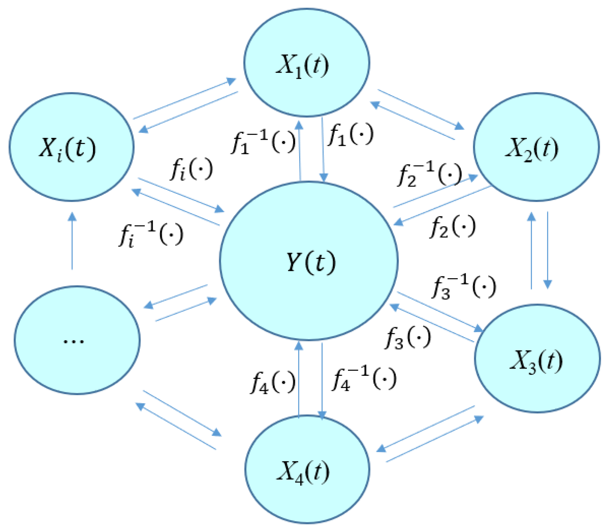
In general, the change in a hydrological variable Y is the result of the influence of multiple factors X1, X2, …, Xi, as shown in Figure 1. Under the condition that the influence of other factors remains unchanged, the effect of single influence factor Xi on the hydrological variable Y is described as a Mechanism function fi(Xi). The Mechanism function, which represents the physical mechanism of hydrological phenomena, will never change. For instance, in the flow discharge Q = AV, A is the cross-sectional area, and V is the flow velocity. When V or A or both change with time, Q(t) also changes with the values of A(t) or V(t) or both, but the Mechanism function or remains unchanged. In other words, V and A may change with time in the specific environment, but the mechanism that the flow discharge equal to the multiplication of these two Mechanism functions will never change. Therefore, the physical mechanism will remain unchanged no matter how the state of Xi changes with time.
According to the above concept of Mechanism function, the relationship model between Y and the Mechanism function of multiple influence factors can be established. Due to the complexity of hydrological systems and the analytical capability, statistical models are usually used to describe the relationship between Y and its explanatory variables. There are two general forms of statistical models: the superposition model and the multiplication model.
where N is the number of influencing factors of hydrological variable Y, and fi(Xi(t)) is the Mechanism function of influencing factor Xi. Assuming that n of N influence factors are known, the effect of the remaining N-n unrecognized influence factors shows randomness and is denoted by . Then, the Equations (1) and (2) can be written as:
Considering the universal interaction among the hydrological elements in the hydrological system, there is no absolute independence among the explanatory variables, and their interactions make the hydrological system exhibit a highly complex nonlinear state. Therefore, the multiplication model is more applicable to describe the hydrological system than the superposition model. Since the nonstationary change of Y(t) is caused by the nonstationary changes in some influencing factors, if the effects of all the nonstationary factors are removed from Y(t), as shown in Equation (5), the remainder will show stationarity.
where m is the number of nonstationary influencing factors. The right side of Equation (5) is the multiplication of the Mechanism functions of the remaining stationary factors and other unrecognized influence factors, which is denoted as , and is usually considered as a natural random variable with a probability distribution characterized by the mean and variance . If only a subset of the nonstationary factor X1, X2, …, Xl (l < m) is considered, it is still a nonstationary series. However, when the most important nonstationary factors are removed, the remaining series can achieve the statistical stationary state. According to the Me-RS idea, the Me-RS function of Y(t) is defined as
The new stationary series reconstructed by the Me-RS function is called the Me-RS series, denoted as RSt. Theoretically, when all the influencing factors causing nonstationary changes in Y are identified (i.e., l = m), and the Mechanism functions are constructed accurately, the Me-RS series (t = 1,2,…) calculated by the Me-RS function is stationary and can be used in any case where a stationary series is required. Although it is impossible to obtain an absolute stationary process due to the limitations of our understandings and existing methods, it is practical to achieve the statistical stationary state. As the correct explanatory variable Mechanism functions are continuously added to the Me-RS function, the Me-RS series will gradually tend to be statistically stationary and closer to a random noise.
Due to the causal relationship between the research variable Y and its influence factors, the nonstationarity (linear, nonlinear, or abrupt change) of the research variable Y is consistent with the corresponding nonstationarity of the influence factors. After removing the influence of the nonstationary factors according to the Me-RS method, the numerical characteristic of the Me-RS series is a constant, i.e.,
Therefore, the Me-RS method is not limited to a specific type of nonstationarity and is effective for any kind of nonstationary change.
2.2. Frequency Analysis of Nonstationary Annual Runoff Series
After obtaining the stationary Me-RS series, the traditional method can be used to conduct the frequency analysis, including the distribution and parameter estimation, and then obtain the design value RSp of the Me-RS series under a certain standard (frequency or return period). Based on the assumption that “the nonstationary change of the hydrological variable Y is caused by the nonstationary change of its influence factor,” as long as the value of the influence factor Xi at a certain time is determined, the design value of the nonstationary annual runoff series Y(t) can be obtained according to the definition of the Me-RS function as follows:
in which the Xi,design is the value of the influence factor at the design stage, which can be the current value or the predicted value.
2.3. Uncertainty Analysis Using the Bootstrap Method
In order to provide relatively robust design results to engineering design and water resources management, it is necessary to evaluate the rationality of the Me-RS method from the perspective of uncertainty of design value. We used the Bootstrap method [27] to quantitatively analyze the uncertainty of the design value, that is, resample the Me-RS series RSt N times to obtain N sample series, calculate the design value RSp,j (j = 1,2,…,N) of each sample series, obtain the design annual runoff Yp,j (j = 1,2,…,N) according to Equation (9), and then deduce the uncertainty confidence interval of design value under the significance level .
2.4. Nonstationary Analysis
Strictly speaking, the Mechanism function should be determined by theoretical derivation or experimental analysis. However, due to the complexity of hydrological behaviors and our limited understandings, it is difficult to obtain the absolutely accurate mathematical expressions of the Mechanism function that represents the physical mechanism of hydrological behaviors. Since the influence law between hydrological elements can be implied in the statistical law, the statistical relationship between Y and Xi can be used to estimate the Mechanism function. It is clear that the estimated Mechanism function has certain uncertainty, so the nonstationary test of RSt is necessary. The tests used in this paper include the Mann-Kendall (M-K) test [28,29] for the trend analysis of the first moment, the Pettitt test [30] for the change-point analysis, and the Breusch-Panan (B-P) test [31] for the trend analysis of the second moment. The significance level α of each test is 0.05.
3. Study Area and Data
3.1. Study Area
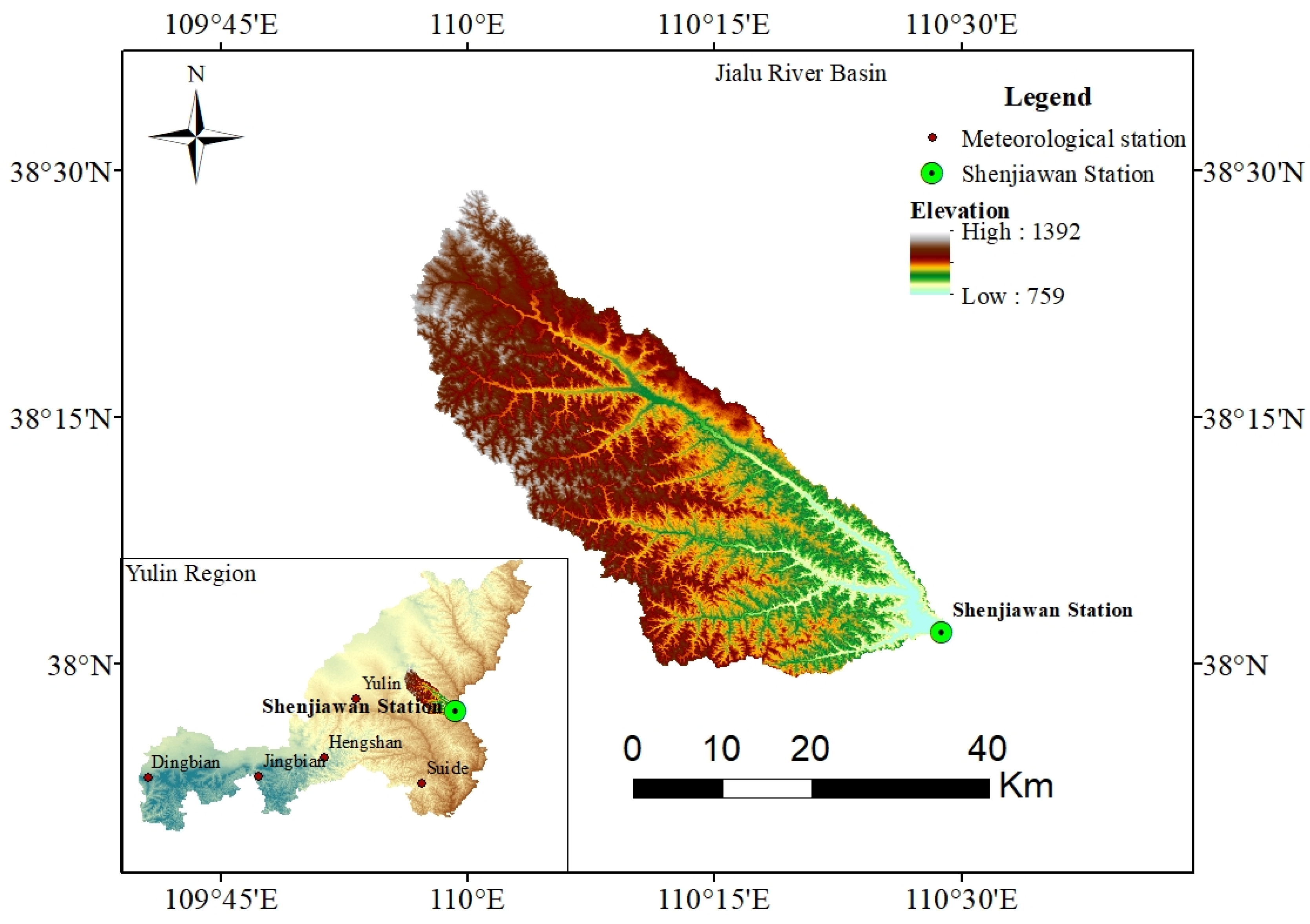
In this paper, we took the JRB in the Yulin region of Shaanxi Province in China as the study area and conducted nonstationary frequency analysis of the annual runoff series by the Me-RS method. The Jialu River is located along the Yellow River between Hekou and Longmen Station and the southern edge of the Mu Us Desert. The river originates from Duanqiao Village, Yulin City, Shaanxi Province, and flows from northwest to southeast and joins the Yellow River at Muchangwan in Jia County. The JRB has an approximate river length of 93 km and a drainage area of 1134 km2 and lies between the geographical coordinates of 37°58′–38°29′ N and 109°56′–110°32′ E (Figure 2). Shenjiawan Hydrological station is the control station for this area. The average annual precipitation in this basin is about 402.3 mm, 75% of which falls during the flood season. Most of the rainfall is in the form of short, intense rainstorms.
3.2. Data
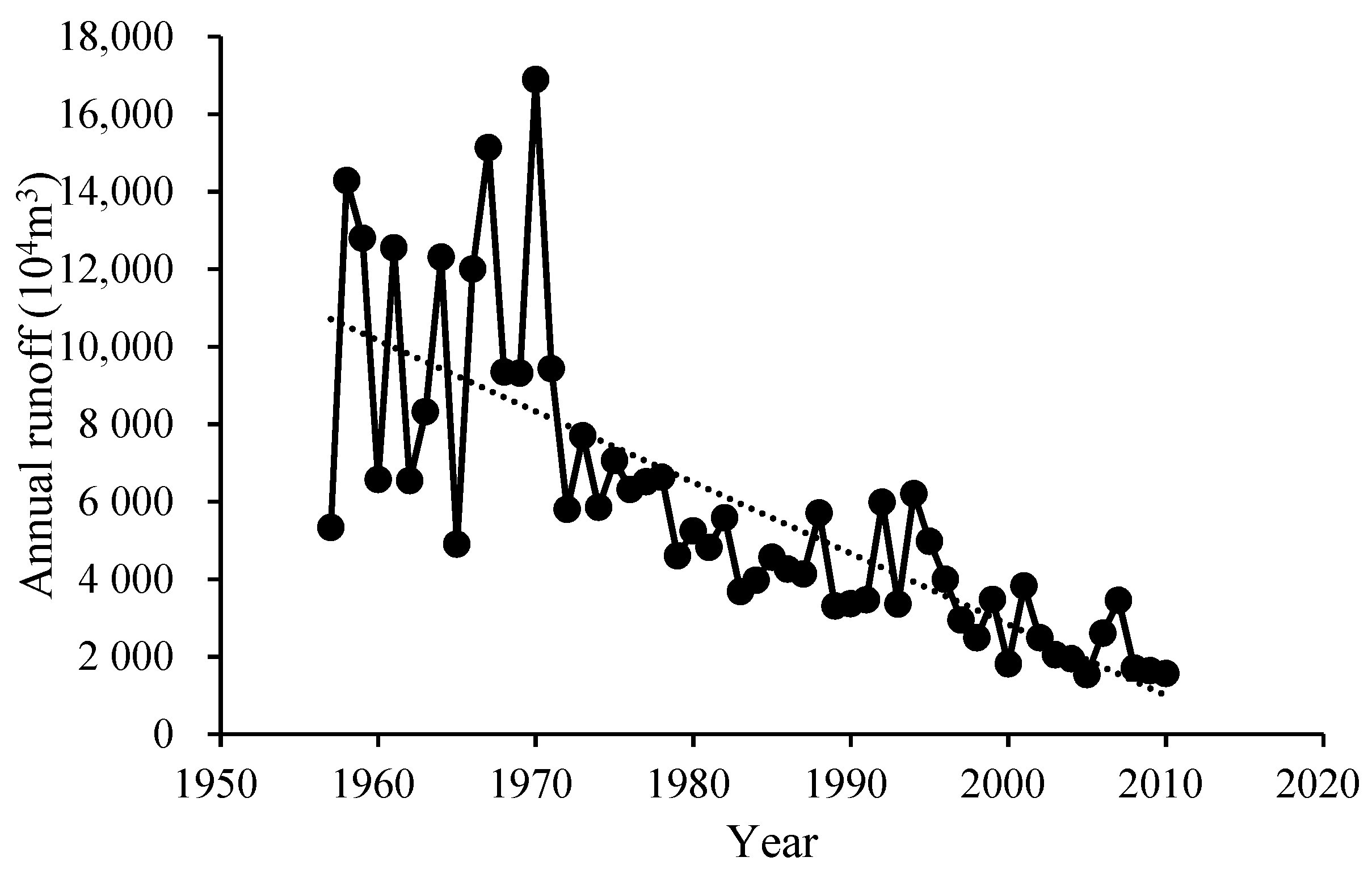
In the Loess Plateau area where the JRB is located, the serious water and soil loss are common. To control this phenomenon, dozens of check dams have been built in JRB. As an engineering measure of water and soil conservation, the check dams can intercept and deposit the sediment in front of the check dams, and the upstream water is slowly drained out by the horizontal pipe. However, in fact, the upstream water is often stored in front of the dam for daily use of residents; that is, the check dam is used as a small reservoir. The number of check dams is very large, with more than 20,000 in Yulin, Shaanxi Province and more than 700 in JRB alone. The continuous construction of the check dam projects results in a continuous downtrend of annual runoff series in JRB, as shown in Figure 3. The nonstationarity test methods in Section 2.4 were adopted to analyze the nonstationarity of the annual runoff series in JRB, as shown in Table 1.
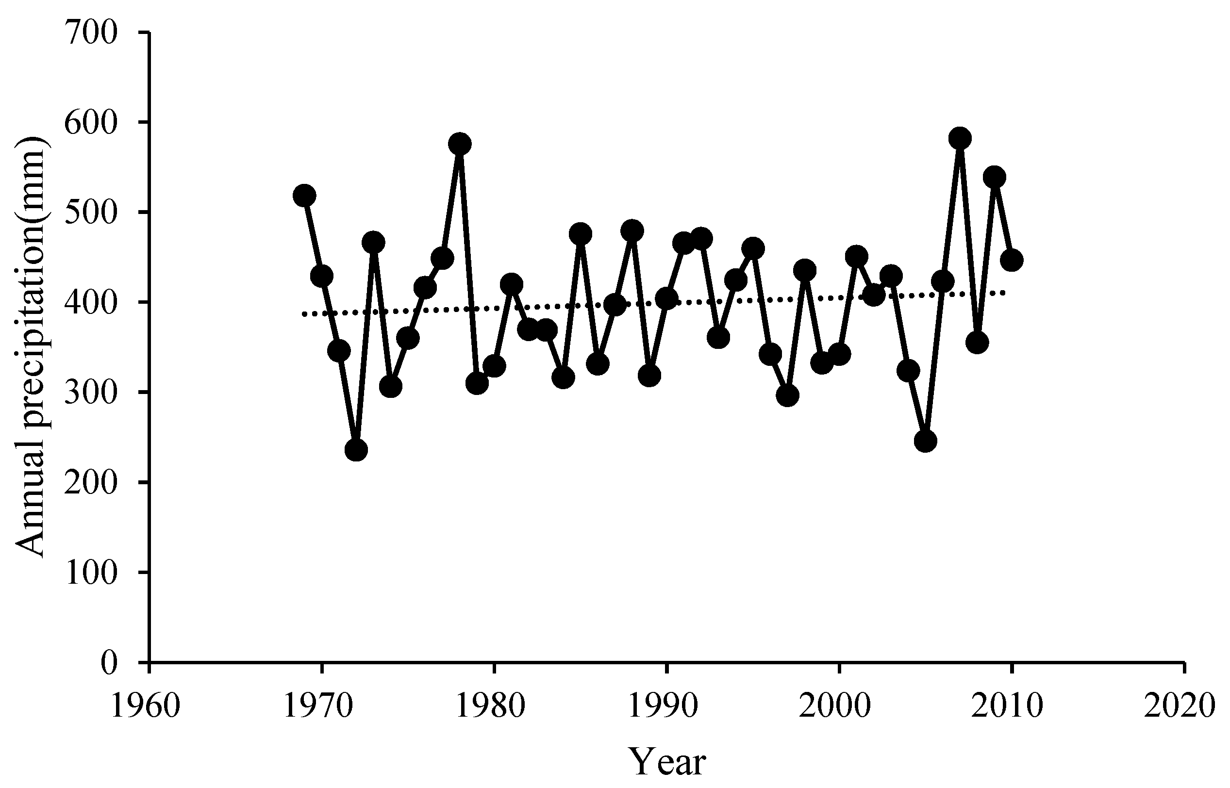
According to Figure 3 and Table 1, the annual runoff series of the JRB exhibits a strong nonstationary change. The first and second moments both show a significant trend, and an abrupt change occurred in 1982. Before the Me-RS analysis of annual runoff series, it is necessary to identify the main influence factors and determine the Mechanism functions. The influencing factors of runoff mainly include climatic factors and underlying surface factors. Among the climatic factors, precipitation is a direct factor affecting the runoff. The annual precipitation series from 1969 to 2010 was collected in this study and is shown in Figure 4. The same nonstationary analysis is shown in Table 1.
According to the test results in Table 1, there is no significant nonstationary change in annual precipitation in JRB, so precipitation is not the main influencing factor causing the nonstationary change in runoff in JRB. Therefore, we turned our attention to the underlying surface factor. Through the field survey, it is concluded that human activities, such as the soil and water conservation engineering measures represented by check dams constructed in JRB in recent years, are the cause of the nonstationarity in annual runoff. The influence of the check dams on the annual runoff is believed to be controlled by the storage capacity and the basin area of the check dams. Therefore, the reservoir index (RI) proposed by López and Francés [11] is used to quantify the impact of check dams.
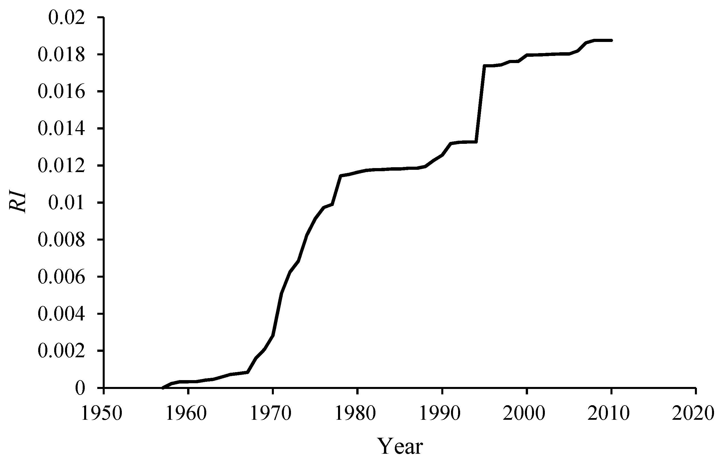
where Ai is the control area of each reservoir, AT is the basin area, Ci is the capacity of each reservoir, CT is the average annual runoff of the basin, and N is the number of reservoir in the basin. The RI series (Figure 5) exhibits a monotonic upward trend.
4. Reconstruction of the Annual Runoff Series
4.1. The Mechanism Function of RI
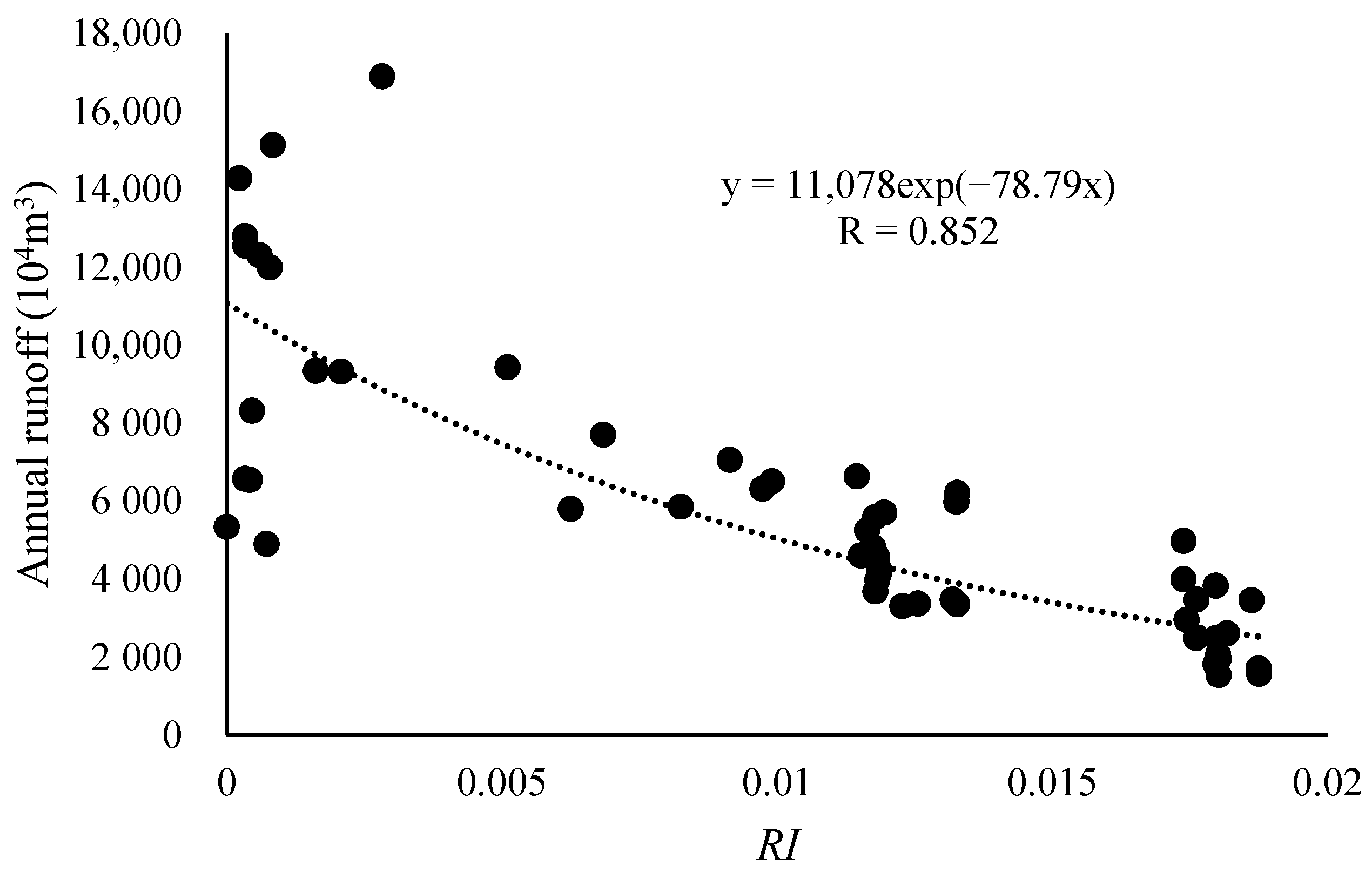
As pointed out in Section 2.4, there are almost no absolutely accurate Mechanism function determined by theoretical derivation or experimental analysis at present. Still, we can estimate the approximation of the Mechanism function one by one through regression approach. We first established the relationship between Y and X1, f1(X1(t)), as the Mechanism function of X1 and then removed the influence of the first factor, i.e., ; then, the Mechanism function f2(X2(t)) of the second factor X2 was established according to the relationship between the remained series and the second factor X2; this process was repeated iteratively until the reconstructed series achieved the stationarity. In the case of this study, RI was taken as the main factor causing the nonstationary change in annual runoff in JRB, and the Mechanism function of RI was estimated by regression analysis, as shown in Figure 6 and Equation (11).
4.2. The Me-RS Function and the Me-RS Series
After obtaining the Mechanism function f(RI), the Me-RS function of the annual runoff in JRB was determined according to Equation (6) as follows:
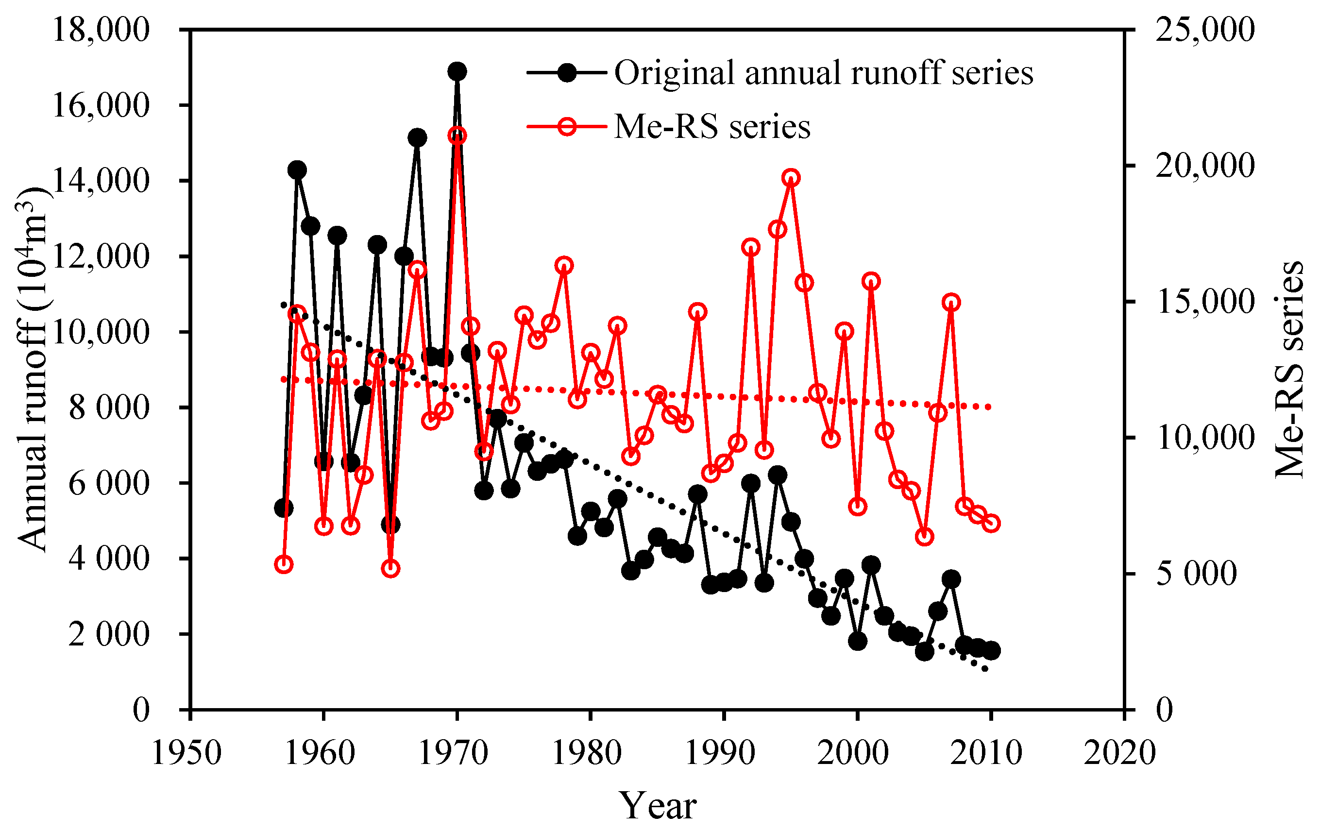
We input the values of annual runoff and RI into the Me-RS function to obtain the Me-RS series of annual runoff, as shown in Figure 7. Since the influence of nonstationary factor RI is removed, the Me-RS series of annual runoff should be stationary; otherwise, other nonstationary factors should continue to be considered. Therefore, the three nonstationary test methods introduced in Section 2.4 were used to analyze the stationarity characteristics of the Me-RS series. The test results are list in Table 2.
Compared with Table 1, after the reconstruction with RI, the original annual runoff series with significant first and second moment trends and significant change-point achieved the stationarity in all aspects, which verified that the Me-RS method is effective for any kind of nonstationary change. In this case, the Me-RS series reconstructed by single-factor RI has excellent stationarity, so no additional factors are added.
5. Frequency Analysis of the Annual Runoff Series
5.1. Calculation of the Design Value of the Me-RS Series
Once the Me-RS series was tested to be stationary, the design value of the Me-RS series could be calculated according to the traditional frequency analysis method. We selected four distributions, the Pearson type III (P-III), Weibull (WEI), Log-normal (LNO), and Gumbel (GU) distributions, as the alternative distributions of the Me-RS series (Table 3).
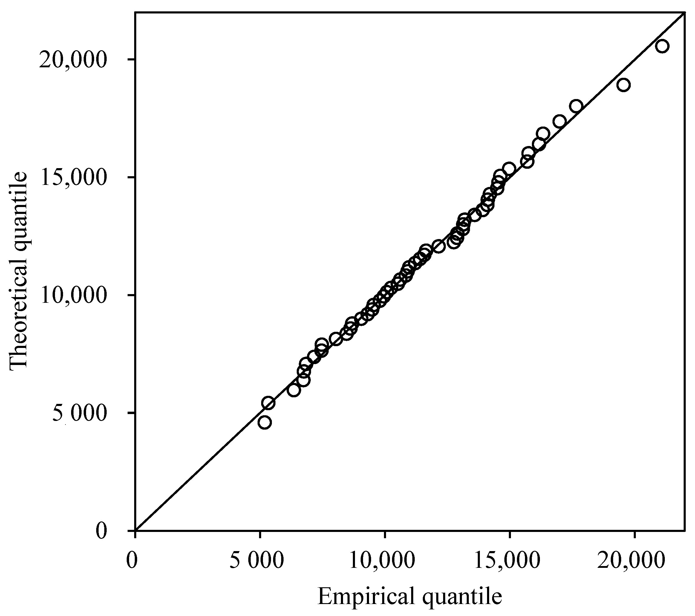
The distribution parameters were estimated by the L-moments method [32]. To evaluate the fitting accuracy of the four alternative distributions, the Kolmogorov-Smirnov test [33], the Nash-Sutcliffe efficiency [34], and the root mean square error were used to determine the optimal distribution. Based on our analysis, the optimal distribution of the Me-RS series of annual runoff in JRB is the WEI distribution (Table 4), and the Q-Q plot in Figure 8 also shows the good fitting effect of WEI distribution.
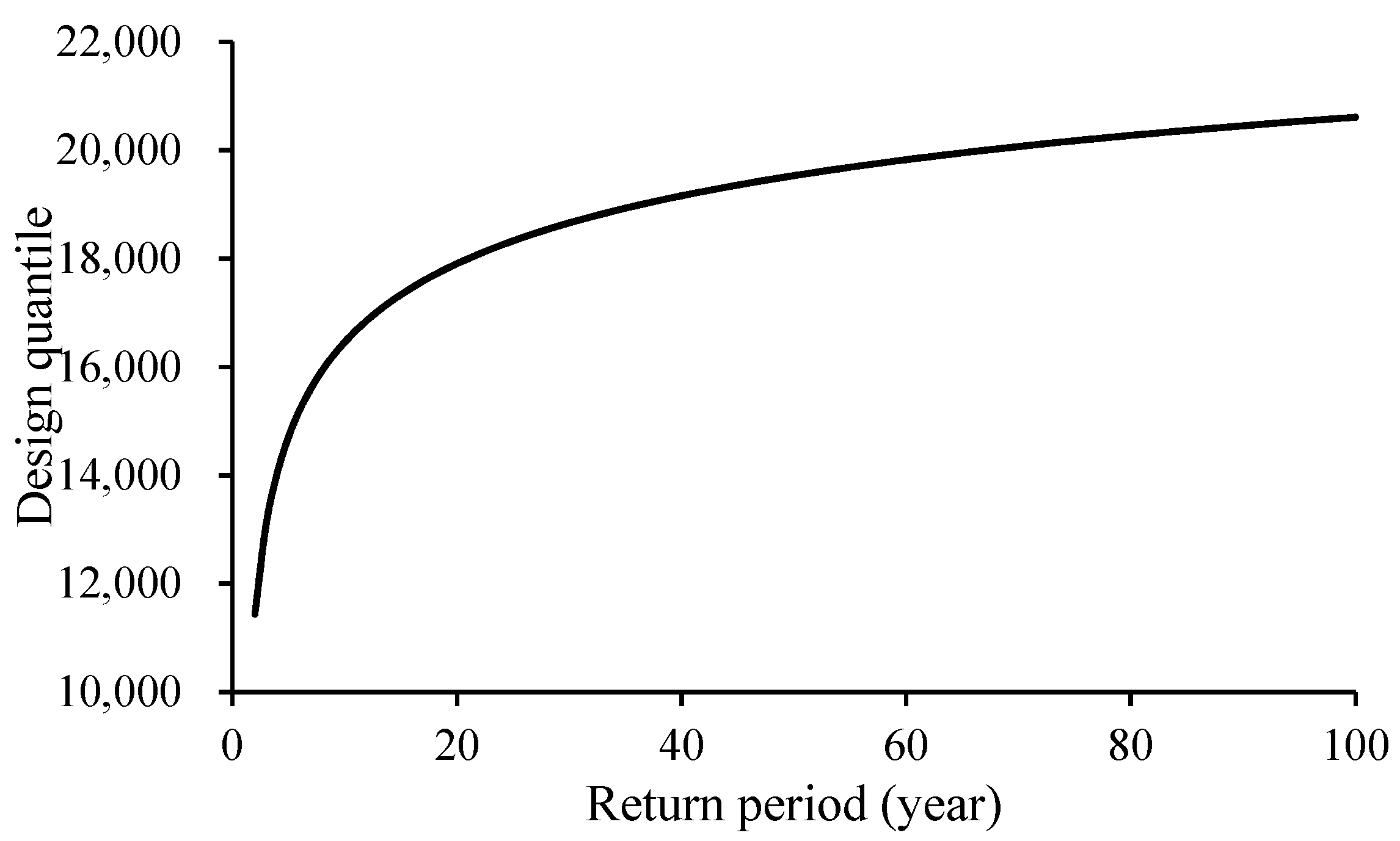
According to the optimal distribution and the estimated parameters, we can determine the design quantiles for various return periods in the Me-RS series (Figure 9).
5.2. Calculation of the Design Annual Runoff
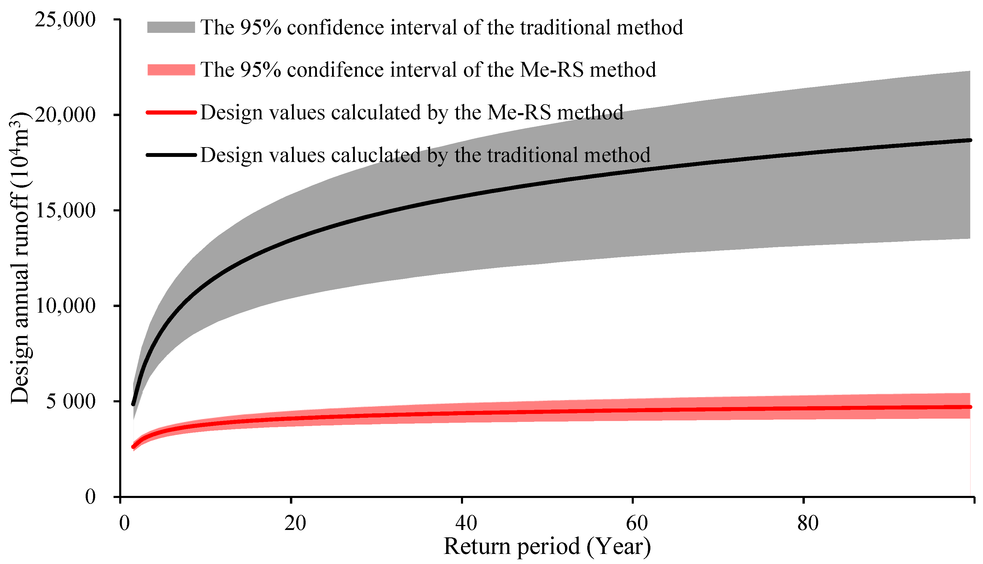
Once the design value of the stationary Me-RS series was calculated, and we could then determine the corresponding quantiles for the original nonstationary annual runoff series according to Equation (9). Therefore, it was necessary to determine the value of the RI at the design stage. Considering that a large number of check dams has been constructed in JRB, and the construction has been saturated in recent years, the RI calculated based on the control area and the storage capacity of the check dams should be basically maintained at the level of 2010, so the RI data in 2010, as shown in Figure 5, were taken as the value at the design stage. Then, according to Equation (9), the design annual runoff is shown in Figure 10.
6. Discussion
6.1. Rationality Analysis of the Design Annual Runoff
The rationality of the design value obtained by the Me-RS method can be analyzed from two aspects. One is from the theoretical perspective: compared with the traditional frequency analysis method, the Me-RS method only conducts the de-nonstationarity transformation on the sample series to ensure that the sample series used for frequency analysis is the simple sample. This method does not change the approaches of estimating the population and calculating the design values. Moreover, the physical meaning of the Me-RS function RS(t) is the research variable under the influence of unit Mechanism function value. Since the design value RSp is only a sample of the RSt population, by using the Equation (9), the RSp is expanded by the Mechanism function value of the design stage, and the obtained design value of the nonstationary annual runoff series is the result of the action of the influence factors under the design conditions. The second method is from the perspective of the design value: as shown in Figure 4 and Figure 5, the precipitation has stayed the same since 1982, but with the continuous construction of the check dams, the water storage volume and the water surface area has gradually increased, resulting in the increase of the total evaporation and the decrease of annual runoff. The average annual runoff measured in recent 30 years and 20 years are 33.7 million m3 and 30.9 million m3, respectively, which is basically equivalent to the 50%-frequency design value 26.1 million m3, indicating that the calculation results are basically consistent with the reality.
6.2. Comparison with the Traditional Frequency Analysis Method
As the current nonstationary frequency analysis theories are far from mature, many hydraulic engineering methods are still designed using the traditional frequency analysis method regardless of whether the sample series is stationary, which is called here the direct traditional frequency analysis method (DTFAM). In order to compare the difference between the Me-RS method and the DTFAM, we also used the DTFAM to calculate the design values of the annual runoff of JRB. The optimal distribution and distribution parameters of the annual runoff series are listed in Table 5. The design values of different return period are shown by the black line in Figure 10. In practice, it is usually necessary to analyze the design values of wet, medium, and dry years, so the results at the frequencies of 20%, 50%, and 80% are list in Table 6. The results of the two methods are greatly different, and the reasons mainly include two aspects. On the one hand, for the Me-RS method, the current RI value is used to calculate the annual runoff design value according to Equation (9). Therefore, the obtained design values reflect the state after the annual runoff series has been reduced. However, the sample series used by the traditional method covers the whole downtrend process of the annual runoff series, which cannot reflect the state of the present stage nor the state of any moment but the average state over the years. On the other hand, the ranking of each sample point has changed after the conversion of the original series to the Me-RS series according to Figure 7. For example, in 1967, from the second place in the original series to the fifth place in the Me-RS series, the change in ranking will also lead to a change in the design value. According to the measured annual runoff data, the design annual runoff at the 50% frequency obtained by the DTFAM is 48.5 million m3, which is 44% or 57% larger than the measure average annual runoff values over recent 30 or 20 years, respectively, and far away from the reality.
According to the Bootstrap method described in Section 2.3, we further analyzed and calculated the uncertainty interval of the design annual runoff deduced by the Me-RS method and the DTFAM, as shown in the shadow in Figure 10. As the return period increases, the uncertainty of the design value increases. However, the uncertainty change rate of the Me-RS method is significantly smaller than that of the DTFAM, and the uncertainty interval width is also far smaller. For the frequency of 50%, the 95% confidence intervals of design value calculated by the DTFAM vary from 40.3 million m3 to 58.9 million m3, and even the lower limit is 19% or 30% larger than the measure average annual runoff values over recent 30 or 20 years, respectively. If the calculation results of DTFAM are used for water resources planning and management, it will have a great impact on water security. It is not consistent with the statistical principle to analyze the nonstationary hydrological series by using the traditional method based on stationary samples, so the obtained design values cannot be guaranteed to conform to the reality. Therefore, the direct use of nonstationary sample series for traditional frequency analysis should be avoided.
6.3. Application Problem of the Me-RS Method
According to the above discussion, the Me-RS method is obviously superior to the DTFAM no matter the theory, the coincidence between the design value and the measured data, or the uncertainty of the design value. The main reason is that the Me-RS method considers the physical cause of nonstationary changes of annual runoff series and obtains the stationary sample series needed for the frequency analysis according to this so as to ensure the correct use of the traditional frequency analysis method. However, the design value is related to the state of the influence factor at the design stage, which brings two problems. First, if the state of the influencing factors changes in the future, then the project constructed at the current stage will inevitably encounter unsuitable problems; for example, the check dams may be continuously silted in the future. Second, changes in some new influencing factors, such as significant changes in rainfall, or in other factors may lead to the unsuitable problem of the projects in the future.
For the first problem, the solution is to recalculate the new Me-RS series according to the changed impact factor. Since the new Me-RS series still reflects the unit action of the original factors, the design value can be recalculated combined with the existing Me-RS series and then according to the new design value to analyze the countermeasures of the hydraulic projects. The second problem can be discussed in two ways. If the new nonstationary influencing factor is a hydrological element with observed data, we only need to reconstruct the annual runoff series by the observed data, then recalculate the design value and analyze the countermeasures of the hydraulic projects. However, if the new factor has never been observed in the past, such as the influence of some human activities that has never occurred, the Me-RS method fails because the influence has not been recorded in history.
Based on the above discussion, it can be concluded that under the nonstationary conditions, all the exiting hydraulic projects will encounter unsuitable problems, and the Me-RS method can provide a reasonable basis for solving this problem.
7. Conclusions
Human activities and climate change lead to nonstationary changes in the originally stationary hydrological series, which brings a theoretical bottleneck to hydrological frequency analysis based on simple samples. As there is no effective solution at present, engineers are still forced to use the traditional frequency analysis method to conduct frequency analysis on the nonstationary hydrological series. However, the results cannot be evaluated, so the safety and economy of the design scheme cannot be judged. The Me-RS proposed in this paper provides an effective tool for annual runoff frequency analysis under nonstationary conditions. The case study on the calculation of design annual runoff in JRB shows that compared with the directly frequency analysis of the nonstationary hydrological series, the Me-RS method not only has theoretical support, but also the obtained design values are consistent with the actual condition and has much smaller uncertainty. Furthermore, the Me-RS method can consider not only the current design conditions but also the future design conditions.
The traditional frequency analysis method is mature in theory and has been tested by engineering practice, while the Me-RS method can achieve good effect because it combines physical cause (Mechanism function) with statistical theory and establishes the Me-RS function according to the Mechanism function of the influence factor, obtains a stationary Me-RS series, and ensures the correct use of the traditional frequency analysis method. It is not consistent with the statistical principle to analyze the nonstationary hydrological series by using the traditional method based on stationary samples, so the obtained design values cannot be guaranteed to conform to the reality. Therefore, the direct use of nonstationary sample series for frequency analysis should be avoided.
Author Contributions
Conceptualization, Y.Q.; methodology, Y.Q. and S.L.; analysis and calculation, S.L.; writing—original draft preparation, S.L.; amending manuscripts, Y.Q.; visualization, S.L.; project administration, Y.Q.; funding acquisition, Y.Q. All authors have read and agreed to the published version of the manuscript.
Funding
This research was funded by National Natural Science Foundation of China, grant number 51679184.
Data Availability Statement
The data presented in this study are available on request from the corresponding author.
Acknowledgments
The field survey of this investigation was carried out as an activity of the Yulin Water Authority of Shaanxi Province, and Yulin Hydraulic engineering design Team for the hydrologic manual revision. Moreover, the observed data were obtained from the team. We would like to express our gratitude and thank all who supported us in this research.
Conflicts of Interest
The authors declare no conflict of interest.
References
- Li, S.; Qin, Y.; Song, X.; Bai, S.; Liu, Y. Nonstationary frequency analysis of the Weihe River annual runoff series using de-nonstationarity method. J. Hydrol. Eng. 2021, 26, 04021034. [Google Scholar] [CrossRef]
- Zhang, Q.; Singh, V.P.; Sun, P.; Chen, X.; Zhang, Z.; Li, J. Precipitation and streamflow changes in China: Changing patterns causes and implications. J. Hydrol. 2011, 410, 204–216. [Google Scholar] [CrossRef]
- Milly, P.C.D.; Dunne, K.A.; Vecchia, A.V. Global pattern of trends in streamflow and water availability in a changing climate. Nature 2005, 438, 347–350. [Google Scholar] [CrossRef] [PubMed]
- Milly, P.C.; Betancourt, J.; Falkenmark, M.; Hirsch, R.M.; Kundzewicz, Z.W.; Lettenmaier, D.P.; Stouffer, R.J. Stationarity is dead: Whither water management? Science 2008, 319, 573–574. [Google Scholar] [CrossRef]
- Strupczewski, W.G.; Singh, V.P.; Feluch, W. Non-stationary approach to at-site flood frequency modelling I. Maximum likelihood estimation. J. Hydrol. 2001, 248, 123–142. [Google Scholar] [CrossRef]
- Strupczewski, W.G.; Kaczmarek, Z.; Feluch, W. Non-stationary approach to at-site flood frequency modelling II. Weighted least squares estimation. J. Hydrol. 2001, 248, 143–151. [Google Scholar] [CrossRef]
- Strupczewski, W.G.; Singh, V.P.; Mitosek, H.T. Non-stationary approach to at-site flood frequency modelling III. Flood analysis of Polish rivers. J. Hydrol. 2001, 248, 152–167. [Google Scholar] [CrossRef]
- Vogel, R.M.; Yaindl, C.; Walter, M. Nonstationarity: Flood magnification and recurrence reduction factors in the United States. J. Am. Water Resour. Assoc. 2011, 47, 464–474. [Google Scholar] [CrossRef]
- Zeng, H.; Feng, P.; Li, X. Reservoir flood routing considering the non-stationarity of flood series in north China. Water Resour. Manag. 2014, 28, 4273–4287. [Google Scholar] [CrossRef]
- Rigby, R.A.; Stasinopoulos, D.M. Generalized additive models for location, scale and shape. J. R. Stat. Soc. Ser. C 2005, 54, 507–544. [Google Scholar] [CrossRef] [Green Version]
- López, J.; Francés, F. Non-stationary flood frequency analysis in continental Spanish rivers, using climate and reservoir indices as external covariates. Hydrol. Earth Syst. Sci. 2013, 17, 3189–3203. [Google Scholar] [CrossRef] [Green Version]
- Xiong, L.; Jiang, C.; Du, T. Statistical attribution analysis of the nonstationarity of the annual runoff series of the Weihe River. Water Sci. Technol. 2014, 70, 939–946. [Google Scholar] [CrossRef] [PubMed]
- Salas, J.D.; Obeyskekera, J. Revisiting the concepts of return period and risk for non-stationary hydrologic extreme events. J. Hydrol. Eng. 2014, 19, 554–568. [Google Scholar] [CrossRef] [Green Version]
- Yan, L.; Xiong, L.; Guo, S.; Xu, C.Y.; Xia, J.; Du, T. Comparison of four nonstationary hydrologic design methods for changing environment. J. Hydrol. 2017, 551, 132–150. [Google Scholar] [CrossRef]
- Villarini, G.; Smith, J.A.; Serinaldi, F.; Bales, J.; Bates, P.D.; Krajewski, W.F. Flood frequency analysis for nonstationary annual peak records in an urban drainage basin. Adv. Water Resour. 2009, 32, 1255–1266. [Google Scholar] [CrossRef]
- Olsen, J.R.; Lambert, J.H.; Haimes, Y.Y. Risk of extreme events under nonstationary conditions. Risk Anal. 1998, 18, 497–510. [Google Scholar] [CrossRef]
- Wigley, T.M.L. The effect of changing climate on the frequency of absolute extreme events. Clim. Change 2009, 97, 67–76. [Google Scholar] [CrossRef]
- Parey, S.; Malek, F.; Laurent, C.; Dacunha-Castelle, D. Trends and climate evolution: Statistical approach for very high temperatures in France. Clim. Change 2007, 81, 331–352. [Google Scholar] [CrossRef] [Green Version]
- Parey, S.; Hoang, T.T.H.; Dacunha-Castelle, D. Different ways to compute temperature return levels in the climate change context. Environmetrics 2010, 21, 698–718. [Google Scholar] [CrossRef]
- Hu, Y.; Liang, Z.; Singh, V.P.; Zhang, X.; Wang, J.; Li, B.; Wang, H. Concept of equivalent reliability for estimating the design flood under non-stationary conditions. Water Resour. Manag. 2018, 32, 997–1011. [Google Scholar] [CrossRef]
- Rootzén, H.; Katz, R.W. Design Life Level: Quantifying risk in a changing climate. Water Resour. Res. 2013, 49, 5964–5972. [Google Scholar] [CrossRef] [Green Version]
- Read, L.K.; Vogel, R.M. Reliability, return periods, and risk under nonstationarity. Water Resour. Res. 2015, 51, 6381–6398. [Google Scholar] [CrossRef]
- Mandelbrot, B.B.; Wallis, J.R. Computer experiments with fractional gaussian noises: Part 1, averages and variances. Water Resour. Res. 1969, 5, 228–241. [Google Scholar] [CrossRef]
- Lins, H.F.; Cohn, T.A. Stationarity: Wanted dead or alive. J. Am. Water Resour. Assoc. 2011, 47, 475–480. [Google Scholar] [CrossRef]
- Serinaldi, F.; Kilsby, C.G. Stationarity is undead: Uncertainty dominates the distribution of extremes. Adv. Water Resour. 2015, 77, 17–36. [Google Scholar] [CrossRef] [Green Version]
- Qin, Y.; Li, S. Study on mechanism-based reconstruction method to cope with the nonstationary change of hydrological series. J. Hydraul. Eng. 2021, 52, 807–818. (In Chinese) [Google Scholar] [CrossRef]
- Efron, B. Bootstrap methods: Another look at the jackknife. Ann. Stat. 1979, 7, 1–26. [Google Scholar] [CrossRef]
- Mann, H.B. Nonparametric tests against trend. Econom. J. Econom. Soc. 1945, 13, 245–259. [Google Scholar] [CrossRef]
- Kendall, M.G. Rank Correlation Methods; Charles Griffin: London, UK, 1975. [Google Scholar]
- Pettitt, A.N. A non-parametric approach to the change-point problem. Appl. Stat. 1979, 28, 126–135. [Google Scholar] [CrossRef]
- Breusch, T.S.; Pagan, A.R. A simple test for heteroscedasticity and random coefficient variation. Econometrica 1979, 47, 1287–1294. [Google Scholar] [CrossRef]
- Hosking, J.R.M. L-moments: Analysis and estimation of distributions using linear combinations of order statistics. J. R. Stat. Soc. Ser. B Methodol. 1990, 52, 105–124. [Google Scholar] [CrossRef]
- Kolmogorov-Smirnov, A.N.; Kolmogorov, A.; Kolmogorov, M. Sulla determinazione empírica di una legge di distribuzione. G. Institto Ital. Attuari 1933, 4, 83–91. [Google Scholar]
- Nash, J.E.; Sutcliffe, J.V. River flow forecasting through conceptual models part I-A discussion of principles. J. Hydrol. 1970, 10, 282–290. [Google Scholar] [CrossRef]
Figure 1.
The relationship between hydrological variable Y and its influencing factors.

Figure 2.
Geographic location of the JRB and meteorological and hydrological data.

Figure 3.
The annual runoff series of the JRB from 1959 to 2010.

Figure 4.
The annual precipitation series of the JRB from 1969 to 2010.

Figure 5.
Time-varying characteristic of the RI series in the JRB.

Figure 6.
The estimated Mechanism function of the RI on the annual runoff.

Figure 7.
Comparison of the Me-RS series and the original annual runoff series in JRB.

Figure 8.
Q-Q plot of the theoretical and empirical quantiles for the Me-RS series of the JRB annual runoff.
Figure 8.
Q-Q plot of the theoretical and empirical quantiles for the Me-RS series of the JRB annual runoff.

Figure 9.
The design quantiles of different return periods of the Me-RS series in JRB.

Figure 10.
The design values of different return periods of the Me-RS series in JRB with the 95% bootstrapped confidence intervals.
Figure 10.
The design values of different return periods of the Me-RS series in JRB with the 95% bootstrapped confidence intervals.


Table 1.
The nonstationary tests of the annual runoff series in JRB.
| Object | M-K Test for Mean | B-P Test for Variance | Pettitt Test for Change Point | |||
|---|---|---|---|---|---|---|
| Z | Change-Point | p-Value | ||||
| Annual runoff series | −7.49 | 1.96 | 23.27 | 3.84 | 1982 | 6.80 × 10⁻⁸ |
| Annual precipitation series | 0.50 | 1.96 | 0.01 | 3.84 | - | - |
Table 2.
The nonstationary tests of the Me-RS series of the annual runoff in JRB.
| Object | M-K Test for Mean | B-P Test for Variance | Pettitt Test for Change Point | |||
|---|---|---|---|---|---|---|
| Z | Change-Point | p-Value | ||||
| Annual runoff series | −7.49 | 1.96 | 23.27 | 3.84 | 1982 | 6.80 × 10⁻⁸ |
| Me-RS series | −0.97 | 1.96 | 0.12 | 3.84 | - | - |
Table 3.
Probability density functions of the alternative distributions.
| Distribution | Probability Density Function |
|---|---|
| P-III | |
| WEI | |
| LNO | |
| GU |
Table 4.
Parameter estimation of the optimal distribution for the Me-RS series of the JRB annual runoff.
Table 4.
Parameter estimation of the optimal distribution for the Me-RS series of the JRB annual runoff.
| Object | Optimal Distribution | Estimated Parameters |
|---|---|---|
| Me-RS series RSRI,t | WEI |
Table 5.
Parameter estimation of the optimal distribution for the original annual runoff series of JRB.
Table 5.
Parameter estimation of the optimal distribution for the original annual runoff series of JRB.
| Object | Optimal Distribution | Estimated Parameters |
|---|---|---|
| Annual runoff series Rt | WEI |
Table 6.
Nonstationary design values and their uncertainties at different frequencies.
| Method | Design Value (Width of 95% Confidence Intervals)/104 m3 | ||
|---|---|---|---|
| Frequency of 20% | Frequency of 50% | Frequency of 80% | |
| Me-RS method | 3357.52 (571.35) | 2610.38 (514.76) | 1920.62 (450.62) |
| Traditional method | 8442.30 (3124.45) | 4845.28 (1866.65) | 2734.43 (1133.84) |
Publisher’s Note: MDPI stays neutral with regard to jurisdictional claims in published maps and institutional affiliations. |
© 2022 by the authors. Licensee MDPI, Basel, Switzerland. This article is an open access article distributed under the terms and conditions of the Creative Commons Attribution (CC BY) license (https://creativecommons.org/licenses/by/4.0/).
Share and Cite
MDPI and ACS Style
Li, S.; Qin, Y. Frequency Analysis of the Nonstationary Annual Runoff Series Using the Mechanism-Based Reconstruction Method. Water 2022, 14, 76. https://doi.org/10.3390/w14010076
AMA Style
Li S, Qin Y. Frequency Analysis of the Nonstationary Annual Runoff Series Using the Mechanism-Based Reconstruction Method. Water. 2022; 14(1):76. https://doi.org/10.3390/w14010076
Chicago/Turabian StyleLi, Shi, and Yi Qin. 2022. "Frequency Analysis of the Nonstationary Annual Runoff Series Using the Mechanism-Based Reconstruction Method" Water 14, no. 1: 76. https://doi.org/10.3390/w14010076
Note that from the first issue of 2016, this journal uses article numbers instead of page numbers. See further details here.