
A Hybrid Model for Streamflow Forecasting in the Basin of Euphrates


1
Department of Civil Engineering, Istanbul Esenyurt University, Istanbul 34510, Turkey
2
Department of Computer Engineering, Gaziantep University, Gaziantep 27470, Turkey
*
Author to whom correspondence should be addressed.
Water 2022, 14(1), 80; https://doi.org/10.3390/w14010080
Submission received: 28 November 2021
/
Revised: 20 December 2021
/
Accepted: 31 December 2021
/
Published: 3 January 2022
(This article belongs to the Special Issue Advances in Water Use Efficiency in a Changing Environment)
Abstract
:River flow modeling plays a crucial role in water resource management and ensuring its sustainability. Therefore, in recent years, in addition to the prediction of hydrological processes through modeling, applicable and highly reliable methods have also been used to analyze the sustainability of water resources. Artificial neural networks and deep learning-based hybrid models have been used by scientists in river flow predictions. Therefore, in this study, we propose a hybrid approach, integrating long-short-term memory (LSTM) networks and a genetic algorithm (GA) for streamflow forecasting. The performance of the hybrid model and the benchmark model was taken into account using daily flow data. For this purpose, the daily river flow time series of the Beyderesi-Kılayak flow measurement station (FMS) from September 2000 to June 2019 and the data from Yazıköy from December 2000 to June 2018 were used for flow measurements on the Euphrates River in Turkey. To validate the performance of the model, the first 80% of the data were used for training, and the remaining 20% were used for the testing of the two FMSs. Statistical methods such as linear regression was used during the comparison process to assess the proposed method’s performance and to demonstrate its superior predictive ability. The estimation results of the models were evaluated with RMSE, MAE, MAPE, STD and R2 statistical metrics. The comparison of daily streamflow predictions results revealed that the LSTM-GA model provided promising accuracy results and mainly presented higher performance than the benchmark model and the linear regression model.
1. Introduction
Water is one of the most crucial resources for the survival of all living creatures on Earth. Since the amount of water on Earth is constant, the need for water increases in line with the population rate. Therefore, planning and managing water resources as accurately as possible has recently become one of the essential issues in hydrology.
Global warming, drought and their effects on the water level ultimately negatively impact humans’ lives. Therefore, the existence and quality of water, which is necessary in every aspect of human life, is crucial [1]. Increasing water demand due to drought, climate change, unplanned consumption, industrialization and agricultural use puts pressure on clean water resources. One of the critical measures required to ensure sustainability is forecasting river flows.
Due to the importance of accurate analysis and infrastructure planning in water and energy systems, the need for a higher temporal resolution in water supply and demand analysis and modeling has increased. In recent years, researchers have increased their work on artificial-intelligence-based models in order to determine stream flows stably. Therefore, developing a suitable method to predict the flow rate is crucial and can mitigate the consequences of water demand and supply [2].
In recent years, artificial neural networks (ANN) have been applied in various hydrological processes, such as hydrology, water resources and river engineering. A series of ANN-based studies have presented an efficient approach for flow prediction, precipitation and water quality predictions in terms of accuracy and applicability [3]. Studies have consistently proven that due to the participation of natural variables, predicting flow is a complex task, due to factors such as the complexity of the river system, non-linearity, randomness and non-stationarity [4,5]. Nowadays, we often see neural networks implemented to provide technological solutions in our daily life. ANNs have advantages, such as their ability to model non-linearity, as well as their application in the areas of learning, generalization, adaptation, data processing, and hardware. ANNs are able to process the most complex non-linear time series. Consequently, ANs prediction models could provide better yields than statistical and physical methods. High-level programming languages such as MATLAB, Python, NeuroSolutions, etc., are effective and successful used as a toolbox [6]. A literature review reveals that it is possible to model flow models using artificial intelligence (AI) models rather than physically-based models [7]. Models such as recurrent neural networks (RNNs), particle swarm optimization (PSO), genetic algorithms (GAs), and long short-term memory (LSTM) are among the universal computational models used for flow prediction in the field of hydrology [8,9,10]. In addition, there are many difficulties with these models, especially in river engineering applications [11]. Each method has a particular form that can be used to learn a streamflow design and provide forecasts. However, due to the complexity of flow data, accurate prediction has been a significant challenge for decades (particularly as the forecasting time horizon rises). The literature demonstrates that selecting a single model or method with an appropriate performance is tough, and these methods depend on the study area’s location and conditions. Given all the complexities associated with streamflow estimation, having sound knowledge of this variable and an accurate analysis of its variations is inevitably required in order to gain a hydrological understanding of catchment areas by combining models.
Different hybrid models combining ANNs with various optimization techniques have been developed with the aim of selecting the optimal parameters necessary for forecasting different processes related to hydrology and other field of studies. Many deep learning (DL) algorithms, such as RNNs, show great potential in streamflow forecasting. Specifically, in order to use time series, RNN networks have strong learning capabilities. Furthermore, RNNs contain loops that carry information from the previous stage to the next stage in the neural network, but the main problem with RNNs is the vanishing gradient and long sequences dependency. Hochreiter and Schmidhuber [12] developed the LSTM method to overcome the traditional problems of RNNs. LSTM can manage longer-term data than RNNs and can deal with disadvantages of RNNs such as exploding and vanishing gradients. Nowadays, LSTM-based methods have become popular in many fields. LSTM is generally preferred in many sequential models that also contain image captioning, natural language processing and motion detection [13,14,15,16]. Furthermore, unlike traditional ANN models, the LSTM model includes entrance, exit and forgetting doors. The presence of these gates prevents network crashes in the LSTM model and allows it to be reset at the appropriate time [17,18]. LSTM is a common method used to predict diverse time series such as groundwater grades, basin flow and meteorological problems [19,20].
Xu et al. [21] used an LSTM network targeting the time series data field for the flow estimation of rivers. LSTM predictions were compared with support vector regression (SVR) and multilayer perceptron (MLP) models. In addition, extended experiments were conducted on the LSTM model and the factors affecting its performance were investigated. It was observed that the LSTM demonstrated better performance. Kao et al. [22] developed a hybrid model based on an LSTM network for stream estimations in the Shihmen Reservoir basin in Taiwan. It appeared that both models generally provided appropriate multi-step forward estimates, and that the new hybrid model not only effectively mimicked the long-term dependence between precipitation and surface flow, but also gave more reliable and accurate flooding predictions.
Wang et al. [23] used daily rainfall and runoff data for the estimation of the impact on a river basin. Models with principal component analysis (PCA) inputs showed better robustness and accuracy performance than models with good manually filtered data. Bai et al. [24] proposed an LSTM model using the stepped-frame approach for daily surface flow estimation. It was observed that LSTM is a valuable approach and works well for daily flow estimation.
Liu et al. [25] created an LSTM network-connected separation model for estimating river flows. The performance of the model was evaluated using the Willmott index. Inputs generated with monthly flow data gave close results between forecasted and observed values. For long-term predictions, the model showed an increased performance.
Latifoğlu and Nuralan [26] used singular spectrum analysis (SSA) and LSTM analysis together, based on the literature, to make river flow estimates, using LSTM networks. A performance analysis of the new model created using SSA for the prediction data was conducted.
Ni et al. [27] are developing two hybrid models based on LSTM for monthly flow and precipitation forecasting in a basin. Wavelet-LSTM (WLSTM) uses three wavelet transformation algorithms for serial separation and implements a combined convolutional neural network to remove convolutional LSTM (CLSTM) timer properties. LSTM was found to be applicable to time series estimation. Fang et al. [28] recommended a local spatial sequential long-term memory neural network (LSS-LSTM) for flood sensitivity forecasting in Shangyou County, China. Using the flood sensitivity estimates of LSTM’s deep learning technique for the forecast model, two optimizations were applied—data boosting and bulk normalization—to further improve the performance of the suggested method. The LSS-LSTM method shows satisfactory predictive performance in terms of accuracy. Ibrahim et al. [29] categorized machine learning into three main categories, together with the optimization techniques, and will next explore the various AI model used for different hydrology fields, along with the most common optimization techniques. Some advantages and disadvantages found through literature reviews were summarized for ease of reference. Finally, future recommendations and overall conclusions drawn from the results of the researchers were included in that study. Al-Saati et al. [30] forecasted monthly streamflow at the downstream section of the Euphrates River by utilizing ARIMA time series models. The results of the study indicated that the traditional Box–Jenkins model was more accurate than the benchmark model in modeling the monthly streamflow of the studied case. Ghaderpour et al. [31] applied least-squares wavelet software (LSWAVE) to estimate the trends and seasonal components of sixty-year-long climate and discharge time series and to study the impact of climate change on streamflow over time. The results highlighted the potential of LSWAVE in analyzing climate and hydrological time series without any need for interpolation, gap-filling or de-spiking. Chong et al. [32] used a comparative method between wavelet transform (WT) and Fourier transform (FT) analyses to perform a time series frequency analysis and assessment for stream flow over the Johor River. The results indicated that the wavelet analysis was more suitable than the Fourier analysis as it exhibited good extraction of the time and frequency characteristics, especially for a nonstationary data series.
LSTM has many parameters that need to be optimized, such as the window size, neurons per layer and number of layers. However, computation and time limitations make it impossible to reach the optimum global region and find the optimum values of parameters. In addition, LSTM network performance sometimes gives unsatisfied results due to the random selection of initialization parameters. Finally, streamflow data that are chaotic and require complex learning algorithms are highly skewed, with several small and large values. In this context, the main contribution is to find the optimum parameters of the LSTM network in order to increase its learning capability. The operation of population-based algorithms with a set of solutions can usually allow to determine the global optimum region quickly. Therefore, in this study these aspects of the LSTM model, which significantly affect the streamflow forecasting model’s performance, are addressed using a population-based GA algorithm. The aim of this study is to suggest the LSTM method that could be used with correct initial weights for decreasing the prediction error of the stream flow. The GA technique is applied to obtain the best solution and optimize the prediction efficiency. The proposed method combined a GA, with its searching ability, and LSTM, with its learning ability through its hidden layers. While GA is responsible for choosing the optimal initial weights, LSTM is responsible for learning [33]. The article is arranged as follows.
In Section 1, general descriptions and a review of studies related to hybrid model predictions and single model mechanisms are provided. Section 2 describes the study region, the dataset, pre-processing design and methods. In this section, the structures of the LSTM model, the GA algorithm and the GA-LSTM model are defined. LSTM was applied to learn current streamflow data from the long-term data and GA was applied to optimize the parameters of LSTM. The experimental analysis results are discussed in Section 3. Conclusions are drawn and recommendations for future studies are made in the subsequent section.
2. Materials and Methods
2.1. Study Region
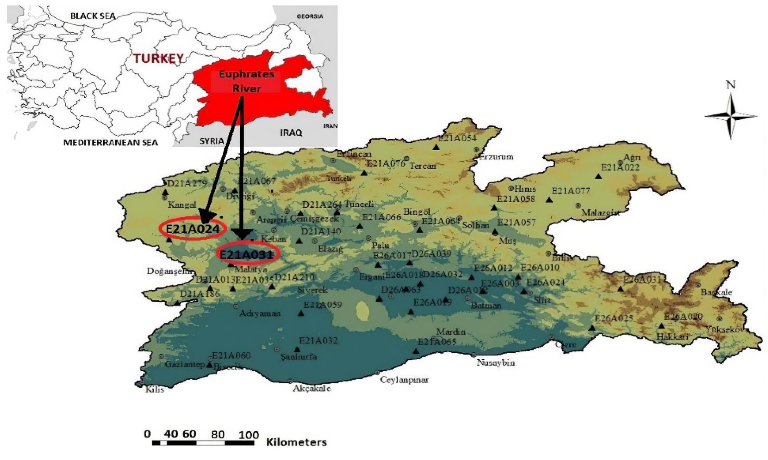
The Euphrates River is the longest in western Asia and has Turkey’s highest productivity and water potential. The majority of the river located in the Turkish territory determines the border of Adıyaman and Gaziantep provinces and passes through Syrian territory and joins in the Persian Gulf. The most critical water resources of the Euphrates are the Tohma, Peri, Karasu, Munzur, Çaltı and Murat streams. Its total length reaches 2800 km within the borders of Turkey (Figure 1). The river regime is more regular than the other streams in Turkey. It carries an average of 30 billion m3 of water annually. It receives 80% of the water it carries from above the Keban dam [34].
2.2. Datasets and Pre-Processing
Long-term 20-year streamflow data were obtained from daily flow measurement stations (FMSs) Beyderesi-Kilayak (E21A31) and Yazıköy (E21A24), shown in Figure 1, which were selected according to the conditions of being on different branches (further upstream) of the Euphrates. These differences are useful in the prediction of river flow regimes. The locations of the stations on the Euphrates River are given with geographical coordinates in Table 1.
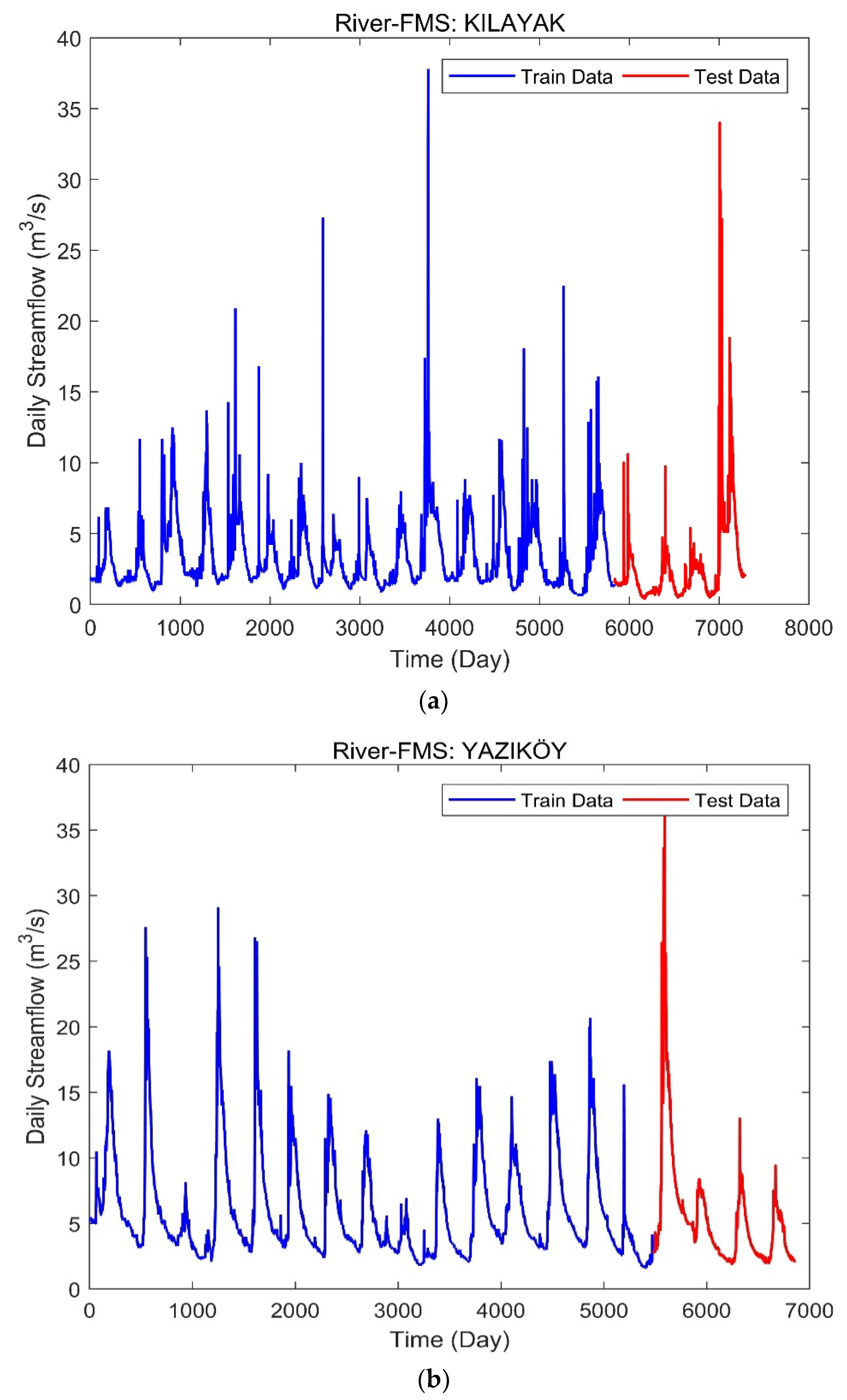
River flow increases significantly in the downstream direction due to surface, subsurface and karst groundwater contributions. As shown in Figure 2, during the observation period, the lowest and highest flows of both stations upstream of the river were 0.44 m3/s and 37.8 m3/s, respectively. Considering the streamflow at Yazıköy FMS, the lowest streamflow was observed to be 1.61 m3/s in 2014 and the highest streamflow was observed to be 37.6 m3/s in 2015. Considering the daily streamflow at the Kılayak FMS, the lowest streamflow was observed in 2016 at 0.44 m3/s and the highest streamflow was observed to be 37.8 m3/s in 2010. The highest streamflow was observed for both stations in the March–May period.
In order to analyze the performance of the hybrid model, initially, Spyder (Python 3.8) was used. In this study, we used the Keras library for training processes and the Deep library to estimate the GA selections. The dataset was directly related to streamflow values for each day. The training process for the proposed method involved 100 epochs for LSTM and a batch size of 8; the optimizer was ADAM and the loss function was MAE. For GA-based selection: the initial population size was 4, the crossover rate was 0.6 and the mutation rate was 0.4 and the number of generations was 10. The performance study used daily flow measurement station data obtained from EIEI (Electrical Works Survey Administration General Directorate). In total, the data consisted of 7304 training days. The data set consisted of a training dataset with 80% of the data and a test dataset with 20%. Furthermore, the hybrid model had two hidden layers. Each layer had 22 memory cells.
The training data were used to examine the indicators in the model and test data were applied for the performance analysis of the comparison and hybrid model. However, the problem of the lack of hydrological data, especially the river flow data, is one of the most crucial problems faced by hydrologists worldwide. These problems arise for many reasons, including technical reasons, and sometimes as a result of unstable situations in a region as a result of conflict or war. Consequently, some historical hydrological data may be available on a river, which may not provide a time series of sufficient flow for the purposes of modern hydrological studies for that river. For this reason, in the selection of data and stations, attention was paid to ensure that data observations were not short- or long-term, but continuous or as little interrupted as possible. In addition, as mentioned above, the features of being in different branches of the river are among the factors to be considered. With these features, E21A31 and E21A24 stations were used to create the datasets for this study. The timespan of the dataset was from September 2000 to June 2019 for Kılayak FMS and the timespan of the dataset was from December 2000 to June 2018. Each record in the dataset contained the streamflow values for daily streamflow.
2.3. Methods
2.3.1. Long-Short-Term-Memory Network
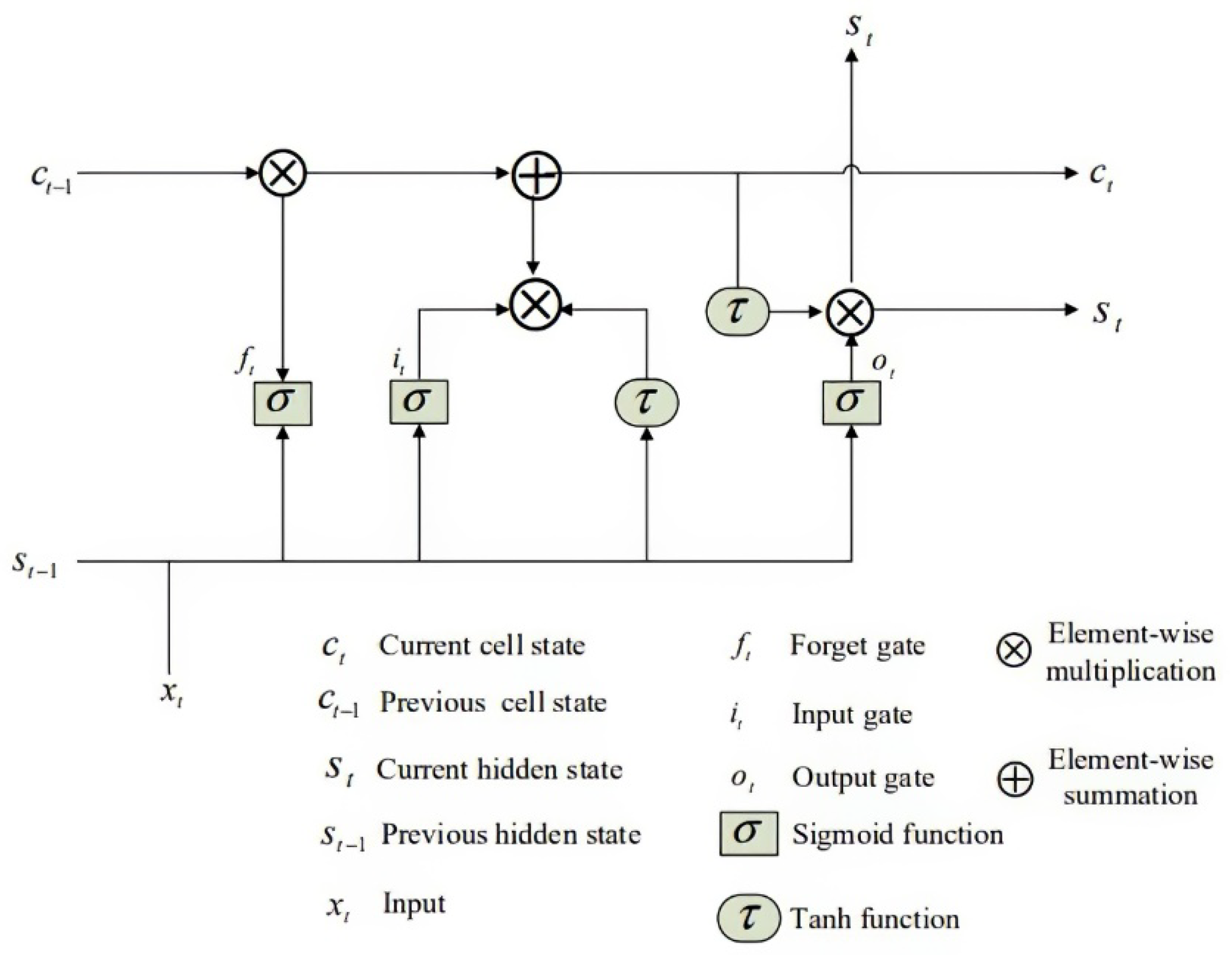
These networks are a specialized version of the recurrent neural network structures that have the ability to recall long-term dependencies while learning the relationships among items. These types of networks are also known for being durable when carrying information over long sequences. LSTM structures are powered by cell states that allow LSTM to transmit information through successor layers. The internal structure of LSTM is composed of three major parts—the input gate, output gate and forget gate—which performs specific operations on cell states. The first submodule, the forget gate, gets rid of the cell state’s irrelevant data. On the other hand, an input gate with a sigmoid (σ) function decides its current information update. Lastly, picking the beneficial information from the overall structure (Figure 3) and exposing it as output data is completed by the output gate [35]. The gates allow the information to be transferred to the next cell state. If the layer generates zero, this means, “do not let any information pass to the next step,” whereas having the value of one as a result of the layer means “let all information pass to the next step” [36].
In Figure 3, three different gates (input gate, forget gate, output gate) and the memory cell of the LSTM cell are depicted. Gate and memory squares indicate matrix multiplication in Equations (1)–(4). Weight(w) and bias(b) are the current values of gates and u indicates a recurrent connection matrix. The slightly distorted ‘s’-shaped cell indicates the sigmoid function indicated in Equation (5), the ‘tanh’ cell indicates the hyperbolic tangent function in Equation (6), the cell with a circle sign indicates the Hadamard product of input matrices, and finally the cell with plus sign indicates the matrix addition operation.
It is possible to add LSTM networks consecutively to create more complex structures. Through this addition process, LSTM can store both the previous records of the first LSTM group and future records of the second LSTM group and make predictions using both types of data. This kind of model can be useful to fill gaps in data such as a missing word in a sentence.
2.3.2. Genetic Algorithm
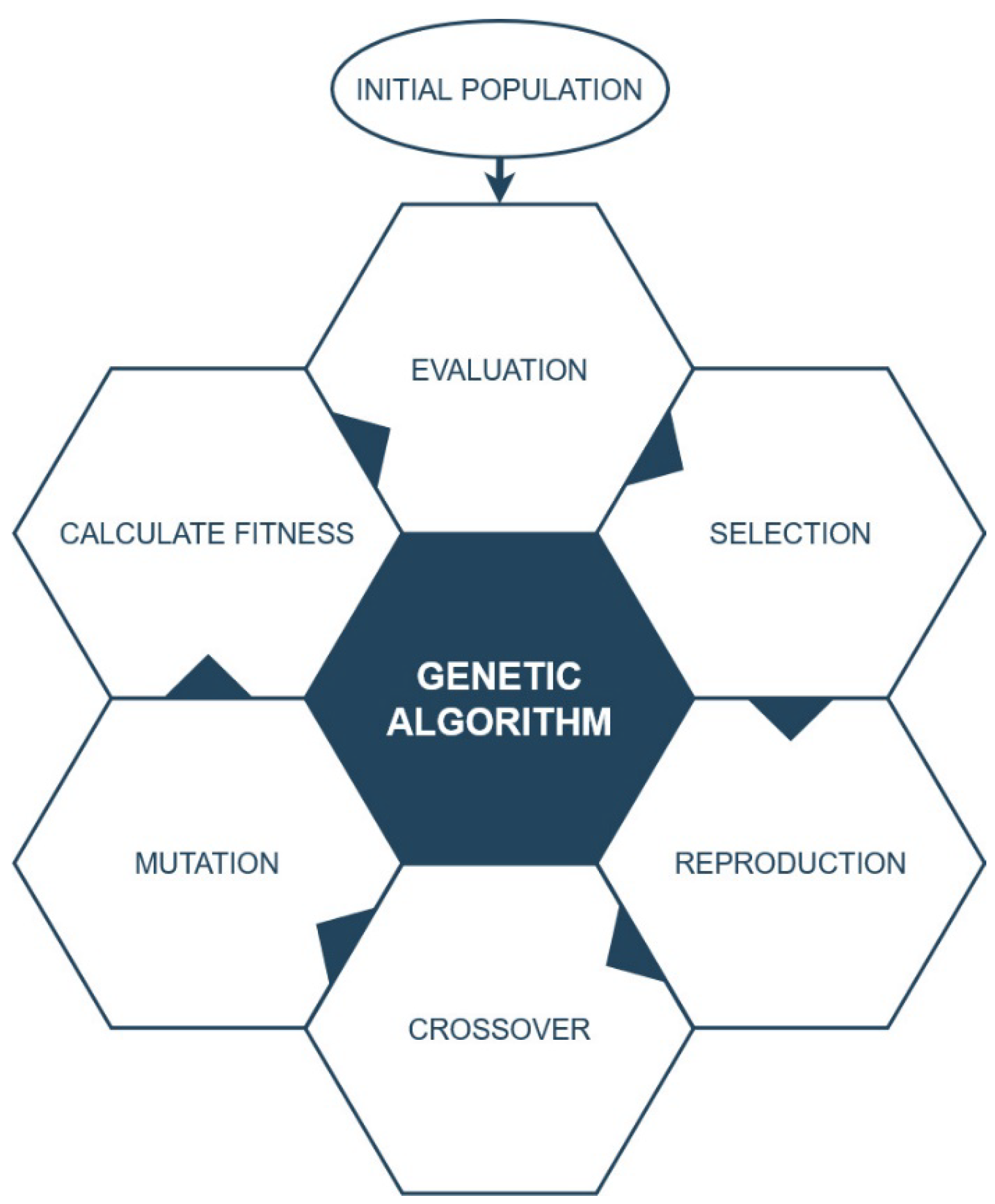
Genetic algorithms (GAs) are inspired by the evolutionary development mechanisms of living things [37]. A GA is a metaheuristic algorithm developed to find the global optimum in the search space. Since it works with a set of solutions, it has the ability to reach the optimal value. Therefore, even in multidimensional problems with a large search space and a large number of variables, the success rate, in terms of obtaining optimal results in acceptable times, is quite high. Operations such as crossover, mutation, evaluation and selection are used to generate optimal new solutions for the fitness function of the problem.
A GA is a population-based optimization algorithm. The candidate solutions that make up the population are the chromosomes in the algorithm [38]. These chromosomes turn into solution candidates that represent better results through various evolutionary processes such as selection, crossover and mutation.
The initial population consists of random candidate solutions. There are no specific criteria for the size of the population. However, it is considered that many individuals in the population do not affect the quality of the solution. The fitness function value indicates the solution quality of each individual. Individuals to be transferred to the next generation are determined according to their fitness function values. In addition, the crossover is usually performed with genes from two- parent chromosomes. This process is applied by replacing the genes from the starting point of the chromosomes up to a point to be determined. The mutation process increases the diversity of chromosomes in the population and provides new solution candidates. Mutation refers the changing of one or more genes of an individual to become a different individual. These processes are shown in Figure 4.
The standard procedure of a GA is to run until an acceptable fitness value is reached or criteria such as a predetermined processing time or number of generations are met. The chromosomes (candidate solutions) used in the evolutionary process are strings that hold variables with discrete or continuous values of the solution they represent [39]. Furthermore, the fitness function is the objective function that measures the quality of chromosomes.
2.3.3. Proposed Method
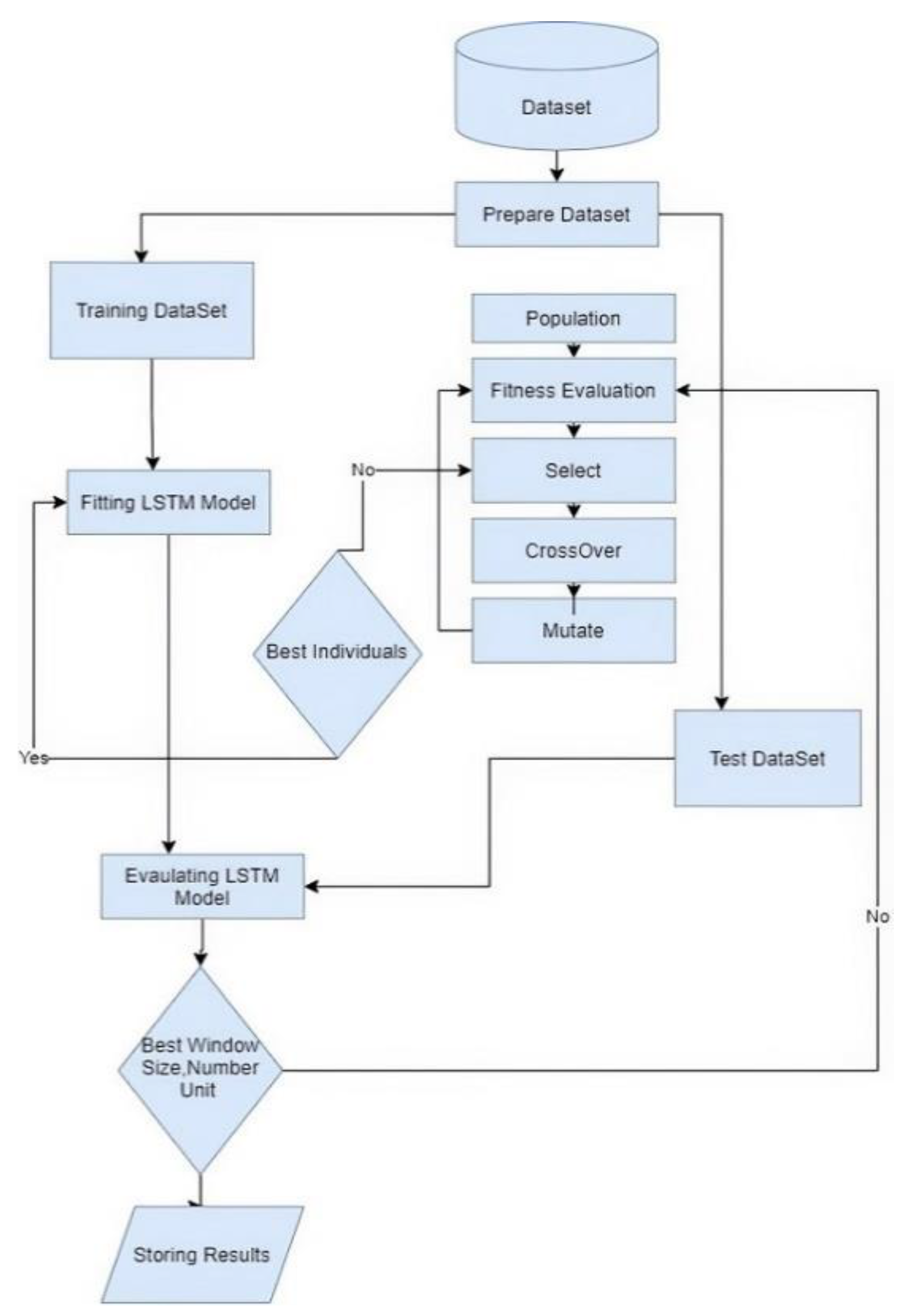
In an LSTM network, in which historical information is essential, the time window is in a critical position. In this study, in order to increase the success of the LSTM network, which is frequently used in river flow time-series predictions, a hybrid model is created by integrating GA optimization into the LSTM network to find the optimum window size and number unit parameters. The success of the model was calculated by comparing its results with those of the non-hybrid model. In order for the comparison data to be healthy and consistent, first of all, the benchmark LSTM model was tested with different parameters and the testing parameters of the best estimation results were taken as a reference. Figure 5 shows the flow of the hybrid model in our study. Accordingly, firstly, the dataset was divided into two groups as test and train. Then, to find the optimum window size and number unit values, GA optimization was run with randomly selected initial population, gene length and number generation values, and the LSTM model was trained and tested for each chromosome until the best individual was found. Afterwards, the results obtained with the optimum window size and number unit values were recorded to be compared with the benchmark model. RMSE was used to calculate the suitability of the chromosomes when creating the GA. The optimal solution was determined by the architectural factors that returned the smallest RMSE.
3. Results and Discussion
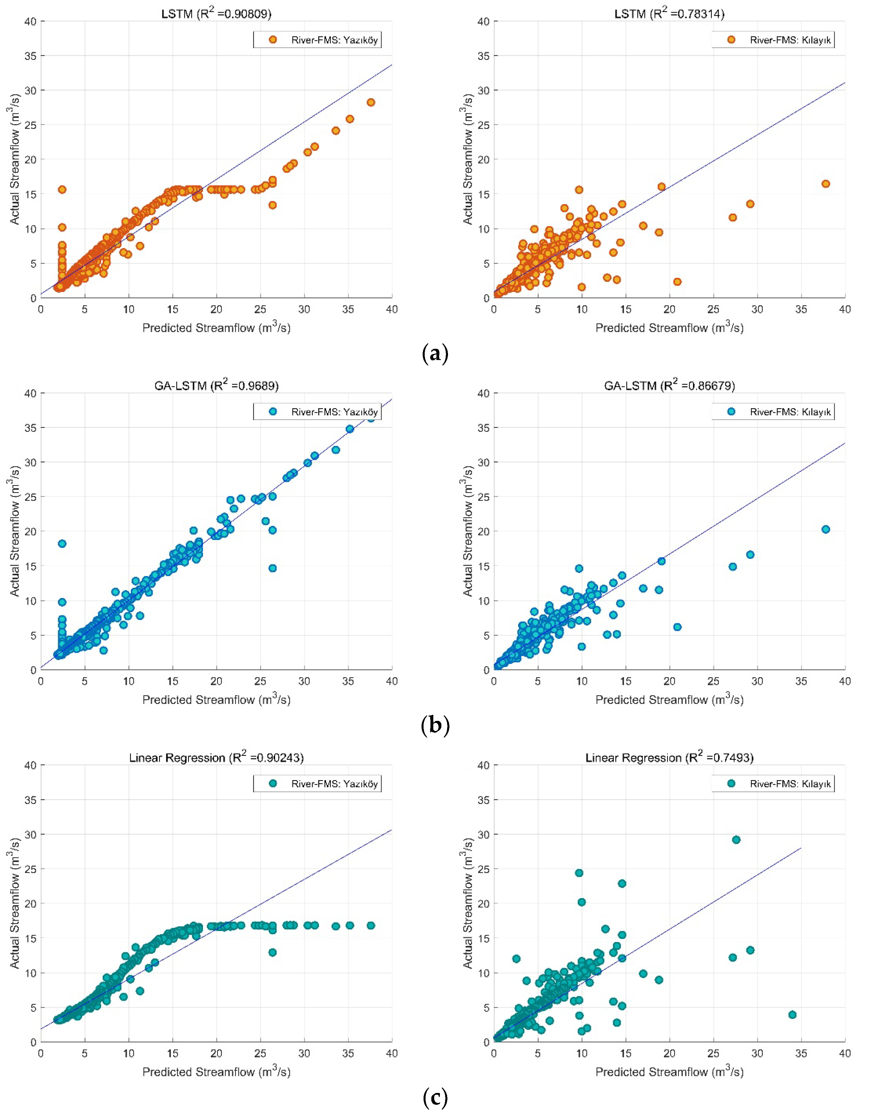
In this section, the performance of the LSTM, the hybrid model and linear regression was analyzed. Test data of streamflow from long-term annual measurements are plotted in Figure 6. It can be seen that the results of the linear regression above only occur when the LSTM performance is analyzed. However, this method inverted to be much more advantageous considering the proposed model’s accuracy, stability and margin of error. The model’s performance was analyzed with 1460 test data for Kilayak FMS and 1357 test data for Yazıköy FMS. The performance of the hybrid model against linear regression seems to be quite successful when the statistical metrics given in Table 2 are examined. Additionally, our aim is to support the results of the statistical measurements of the hybrid and benchmark model included in the study.
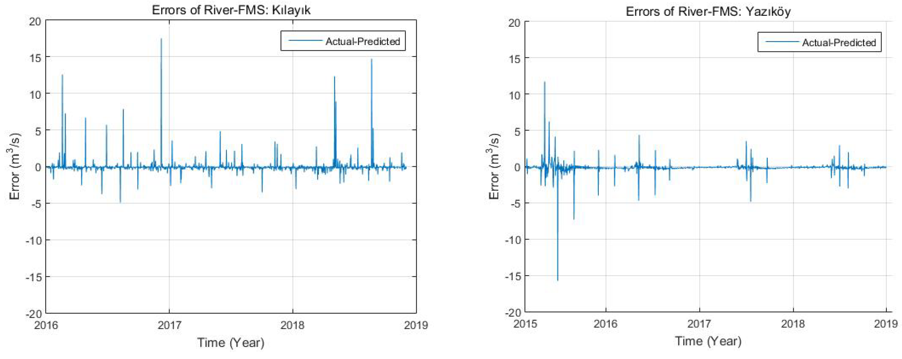
The scatter plots for the GA-LSTM, LSTM and linear regression model for the test data are indicated in Figure 6 to examine the coefficient of determination between the actual and predicted streamflow data. The proposed GA-LSTM method results are close to the actual streamflow data for Kılayak and Yazıköy, although the Yazıköy is normally further upstream. GA-LSTM showed highly successful predictions with an R2 of 0.9689. In the statistical measurement performances of the study, mean absolute deviation (MAD), mean square error (MSE), root mean square error (RMSE), mean absolute error (MAE), mean absolute percentage error (MAPE) and standard deviation (STD) were utilized. These evaluation methods have been widely used in various works and are provided as measurement tools for estimating daily flow values and determining the effectiveness of the model [40,41]. Table 2 shows the statistical measurements of the model results. Furthermore, Table 2 indicates that the proposed model performs better when the error measures are examined. A residual which is also referred as the ‘error value’ can be defined as the difference between the actual data point and the predicted data point. It is a measure of a line of fit for the given regression line and is important for showing model performance. In this context, it is analyzed by its magnitude and whether it forms a pattern when determining the quality of a model. The proposed GA-LSTM method’s residual performance is shown in Figure 7. It is clear that the residual values are too small and that they formed a group.
In the comparison estimations of these three models, In Table 2, in Kılayak FMS the estimated MAE of the LSTM was 0.3976, whereas the estimated MAE of the proposed model was 0.2997, the estimated MAE of the linear regression was 0.3318. The estimation result provided a 75.37% and 90.32% improvement over the benchmark model and linear regression, respectively. The RMSE of the proposed model was found to be 0.9302, whereas that of LSTM was 1.2668 and that of linear regression was 1.3755. The increase in the RMSE value was observed to be 73.42% (benchmark) and 67.62% (linear regression). The MAPE values were found to be 11.5119, 8.9736 and 12.7401 for the benchmark, the proposed model and the linear regression model, respectively. When these values are examined, the increase is seen to be 77.95% over the benchmark and 70.43% over linear regression. The standard deviation values were examined and these values were found to be 0.3359, 0.2152 and 0.3431 for the comparison, suggested and linear models, respectively, and improvements of 64.06% and 62.72% were observed. Finally, according to coefficient of determination (R2), that of the proposed model is found to be 0.8667, whereas that of LSTM was 0.7831 and that of linear regression was 0.7493.
In Yazıköy FMS, the estimated MAE of the LSTM was 0.6615, whereas the estimated MAE of the proposed model was 0.2865 and the estimated MAE of the linear regression was 0.7935. The estimation results provided a 43.31% and 36.10% improvement over the benchmark model and linear regression, respectively. The RMSE of the proposed model was found to be 0.7795, whereas that of LSTM was 1.4316 and that of linear regression was 1.6287. The increase in RMSE value was observed to be 54.44% over the benchmark model and the increase in value was observed to be 47.86% over linear regression. The MAPE values were found to be 17.2010, 5.2819 and 19.2052 for the benchmark, the proposed model and the linear regression model, respectively. When these values are examined, the increase was found to be 30.70% and 27.50% over the benchmark model and linear regression, respectively. The standard deviation values were examined; these values were found to be 0.1913, 0.0973 and 0.1610 for the comparison, suggested and linear models, respectively, and improvements of 50.86% and 60.43% were observed. Finally, the coefficient of determination (R2) of the proposed model was found to be 0.9689, whereas that of LSTM was 0.9060 and that of linear regression was 0.9024.
The hybrid model performed better than the LSTM, revealing the importance of the time window the proper and correct setting of the parameters in order to achieve superior performance. As our results show, there is no need to make large windows for LSTM-based models. However, in MLP models, this proportionally increases the accuracy of the model. Most often, the window is selected depending on the behavior of the predicted signal. It is necessary to choose the size of the window so that one complete cycle of the signal behavior, or a period of time in which the classified signal completely interferes, can fit into this window. Everything described in the study was achieved perfectly, although we tried many possible combinations. Furthermore, the size of the window depends on the sampling frequency or aggregation over time. For example, a 30-min signal can be fit into a window of 60 units if the signal aggregation is performed for 30 s, or in a window of 15 units in size if the aggregation is performed for 2 min. The growth and diversification of learning algorithms make it difficult to search for suitable parameter sets. However, our results indicate that the new hybrid model created herein will provide an effective guide for algorithms and similar data.
The LSTM network is an essential function in determining the performance of prediction models. Combining models such as GA and LSTM seems to provide advantages in time series prediction problems such as river flow predictions. This advantage becomes apparent when the optimization and generation of other units are completed. The proposed hybrid model learned to find the optimal level of river flows and was able to predict the next day’s flow value. This situation is demonstrated by its significant performance when compared to the benchmark model.
This research proves that one can effectively find an optimal result using the GA technique. Experimental results supported this situation and determined the superiority of the proposed hybrid model over the comparison model.
Recently, a number of existing literature studies have been considered the classification of streamflow forecasting using neural networks models.
Thapa et al. [42] developed a deep learning long-short-term memory (LSTM)-based model in the Himalayan basin for snowmelt-based discharge modeling. Fu et al. [43] applied the deep learning method for daily flow simulation, and used data from previous years for flow prediction. The model was carried out according to several perspectives. At the end of the study, it was found that the LSTM model was advantageous in processing constant flow data in the dry season and gave satisfying results in capturing data features in rapidly fluctuating flow data in rainy seasons. Luo et al. [44] built a new hybrid model based on the long-short-term memory approach for predicting streamflow. In this study, the linear regression model, which is one of the classical methods, was used to show how successful the performance between the benchmark model and the hybrid model was. The results obtained via linear regression are shown in Figure 6 as a plotting graph, along with other outputs. When the statistical measurement metrics are examined in Table 2, it is observed that the linear regression approach was weak in both stations, compared to the LSTM. The results have shown that the hybrid model has better performance than the benchmarked model, providing forecast precision.
This study proves that in LSTM-based estimation processes, the use of a GA helps to determine the critical points of window size and the number of units, strengthens the model and improves the results considerably. This hybrid deep learning model is one of the most optimal solutions for solving complex and large-scale data problems.
4. Conclusions
In conclusion, a hybrid method that integrated a GA and LSTM is suggested to forecast streamflow data. The proposed method’s performance was tested on streamflow data from the Euphrates River in western Asia. The results achieved with the GA-LSTM method were equated with the primary LSTM method results. Although the basic LSTM shows robust learning capability for time series, its performance sometimes gives unsatisfactory results due to the random selection of initialization parameters. Due to the operation of population-based algorithms with a set of solutions, GA algorithms usually quickly identify the global optimum region. Therefore, a GA was used to search for suitable values of LSTM parameters in this study. Statistical measurement performances such as MSE, RMSE, MAE and MAPE are essential parameters to evaluate the method’s performance, especially for forecasting measures. In this context, the measures mentioned above were used to evaluate the proposed method. The obtained results showed that the prediction error of the stream flow data was more successfully decreased with the proposed GA-LSTM approach than the benchmark model. Consequently, it was found that our approach had low measures, and these results were statistically significant. In addition, the achieved results indicate that our approach can successfully improve the predictive performance of the basic LSTM.
Furthermore, the data had low standard deviation values in this study. The low standard deviation indicates that the measurement performances values were close to each other, which means that the results are reliable. In addition, the coefficient of determination (R2) was utilized to measure the proposed model’s performance. The results given in Table 2 indicate how well the model fit the data. In general, the high number of parameters to be determined and the starting of the training of the network from a random point were the negative factors. A long computational time is often required to access the region of the global optimum due to high probability-based search strategies for population-based algorithms. In this context, future studies are planned to train the LSTM network using other meta-heuristic searching techniques and to examine its performance on related problems. On the other hand, new regions which have different streamflow characteristics can be analyzed by using the GA-LSTM method. Thus, future research directions can be determined by observing data with different characteristics.
Author Contributions
H.C.K. and B.H. prepared the original draft and reviewed and improved the manuscript. All authors have read and agreed to the published version of the manuscript.
Funding
This research did not receive any specific grant from funding agencies in the public, commercial or not-for-profit sectors.
Institutional Review Board Statement
Not applicable.
Informed Consent Statement
Not applicable.
Data Availability Statement
Not applicable.
Conflicts of Interest
The authors declare no conflict of interest.
Abbreviations
| LSTM | Long-Short-Term Memory |
| ANN | Artificial Neural Network |
| RNN | Recurrent Neural Network |
| PSO | Particle Swarm Optimization |
| DL | Deep Learning |
| MLP | Multi-Layered Perceptron |
| SVR | Support Vector Regression |
| PCA | Principal Component Analysis |
| SSA | Singular Spectrum Analysis |
| WLSTM | Wavelet Long-Short-Term Memory Networks |
| LSSLSTM | Local Spatial Sequential Long-Short Term Memory Networks |
| LSS | Least-Squares Spectrum |
| LSWAVE | Least-Squares Wavelet Software |
| WT | Wavelet Transform |
| FT | Fourier Transform |
References
- Dalkiliç, H.Y.; Hashimi, S.A. Prediction of daily streamflow by using artificial neural networks (ANNs), wavelet neural networks (WNNs), and adaptive neuro-fuzzy inference system (ANFIS) models. Water Supply 2020, 20, 1396–1408. [Google Scholar] [CrossRef] [Green Version]
- Kılınç, H.Ç. Prediction of River Flows using Deep Learning and the Effect of Flows on Railways Routes. J. Railw. Eng. 2021, 13, 106–114. [Google Scholar]
- Şirin, E. Design of Coastal Structures and Estimation of Wave Height by Artificial Intelligence and Time Series Methods. Ph.D. Thesis, Konya Teknik University, Konya, Turkey, 2021. [Google Scholar]
- Yaseen, Z.M.; El-Shafie, A.; Jaafar, O.; Afan, H.A.; Sayl, K.N. Artificial intelligence-based models for stream-flow forecasting: 2000–2015. J. Hydrol. 2015, 530, 829–844. [Google Scholar] [CrossRef]
- Smith, D.M.; Cusack, S.; Colman, A.W.; Folland, C.K.; Harris, G.R.; Murphy, J.M. Improved Surface Temperature Prediction for the Coming Decade from a Global Climate Model. Science 2007, 317, 796–799. [Google Scholar] [CrossRef] [Green Version]
- Bach, H.; Clausen, T.J.; Dang, T.T.; Emerton, L.; Facon, T.; Hofer, T.; Lazarus, K.; Muziol, C.; Noble, A.; Schill, P.; et al. From Local Watershed Management to Integrated River Basin Management at National and Transboundary Levels; Watershed Management Scientific Report; Mekong River Commission: Vientiane, Laos, 2011; Volume 1, pp. 4–5. [Google Scholar]
- Shamshirband, S.; Rabczuk, T.; Chau, K.-W. A survey of deep learning techniques: Application in wind and solar energy resources. IEEE Access 2019, 7, 164650–164666. [Google Scholar] [CrossRef]
- Ahi, Ş.N.; Soğukpınar, I.I. Phishing e-mail detection with deep learning models. J. BBMD 2020, 13, 17–31. [Google Scholar]
- Mehr, A.D.; Nourani, V.; Kahya, E.; Hrnjica, B.; Sattar, A.M.; Yaseen, Z.M. Genetic programming in water resources engineering: A state-of-the-art review. J. Hydrol. 2018, 566, 643–667. [Google Scholar] [CrossRef]
- Bowden, G.J.; Dandy, G.C.; Maier, H.R. Input determination for neural network models in water resources applications. Part 1—Background and methodology. J. Hydrol. 2015, 301, 75–92. [Google Scholar] [CrossRef]
- Wang, W.-C.; Chau, K.-W.; Xu, D.-M.; Qiu, L.; Liu, C.-C. The annual maximum flood peak discharge forecasting using hermite projection pursuit regression with SSO and LS method. Water Resour. Manag. 2017, 31, 461–477. [Google Scholar] [CrossRef]
- Hochreiter, S.; Schmidhuber, J. Long short-term memory. Neural Comput. 1997, 9, 1735–1780. [Google Scholar] [CrossRef]
- Santra, A.S.; Lin, J.-L. Integrating Long Short-Term Memory and Genetic Algorithm for Short-Term Load Forecasting. Energies 2019, 12, 2040. [Google Scholar] [CrossRef] [Green Version]
- Sutskever, I.; Vinyals, O.; Le, Q.V. Sequence to sequence learning with neural networks. In Proceedings of the Advances in Neural Information Processing Systems, Montreal, QC, Canada, 8–13 December 2014; pp. 3104–3112. [Google Scholar]
- Khan, S.; Yairi, T.A. Review on the application of deep learning in system health management. Mech. Syst. Sig. Process. 2018, 107, 241–265. [Google Scholar] [CrossRef]
- Zhou, X.; Tang, Z.; Xu, W.; Meng, F.; Chu, X.; Xin, K.; Fu, G. Deep learning identifies accurate burst locations in water distribution networks. Water Resour. 2019, 166, 115058. [Google Scholar] [CrossRef]
- Kühnert, C.; Gonuguntla, N.M.; Krieg, H.; Nowak, D.; Thomas, J.A. Application of LSTM Networks for Water Demand Prediction in Optimal Pump Control. Water 2021, 13, 644. [Google Scholar] [CrossRef]
- Gers, F.A.; Schmidhuber, J.; Cummins, F. Learning to forget: Continual prediction with LSTM. Neural Comput. 2000, 12, 2451–2471. [Google Scholar] [CrossRef]
- Fotovatikhah, F.; Herrera, M.; Shamshirband, S.; Chau, K.-W.; Ardabili, S.F.; Piran, M.J. Survey of computational intelligence as basis to big flood management: Challenges, research directions and future work. Eng. Appl. Comput. Fluid Mech. 2018, 12, 411–437. [Google Scholar] [CrossRef] [Green Version]
- Mitchell, M. An Introduction to Genetic Algorithms; MIT Press: Cambridge, MA, USA, 1998. [Google Scholar]
- Xu, W.; Jiang, Y.; Zhang, X.; Li, Y.; Zhang, R.; Fu, G. Using long short-term memory networks for river flow prediction. Hydrol. Res. 2020, 51, 1358–1376. [Google Scholar] [CrossRef]
- Kao, I.F.; Zhou, Y.; Chang, L.C.; Chang, F.J. Exploring a Long Short-Term Memory based Encoder-Decoder framework for multi-step-ahead flood forecasting. J. Hydrol. 2020, 583, 124631. [Google Scholar] [CrossRef]
- Bai, Y.; Xie, J.; Liu, C.; Tao, Y.; Zeng, B.; Li, C. Regression modeling for enterprise electricity consumption: A comparison of recurrent neural network and its variants. Int. J. Electr. Power Energy Syst. 2020, 126, 106612. [Google Scholar] [CrossRef]
- Wang, Q.; Liu, Y.; Yue, Q.; Zheng, Y.; Yao, X.; Yu, J. Impact of Input Filtering and Architecture Selection Strategies on GRU Runoff Forecasting: A Case Study in the Wei River Basin, Shaanxi, China. Water 2020, 12, 3532. [Google Scholar] [CrossRef]
- Bai, Y.; Bezak, N.; Zeng, B.; Li, C.; Sapač, K.; Zhang, J. Daily Runoff Forecasting Using a Cascade Long Short-Term Memory Model that Considers Different Variables. Water Resour. Manag. 2020, 35, 1167–1181. [Google Scholar] [CrossRef]
- Liu, D.; Jiang, W.; Mu, L.; Wang, S. Streamflow Prediction Using Deep Learning Neural Network: Case Study of Yangtze River. IEEE Access 2020, 8, 90069–90086. [Google Scholar] [CrossRef]
- Latifoğlu, L.; Nuralan, K.B. River Flow Prediction with Singular Spectrum Analysis and Long Short-Term Memory Networks. Eur. J. Sci. Technol. 2020, 1, 376–381. [Google Scholar] [CrossRef]
- Ni, L.; Wang, D.; Singh, V.P.; Wu, J.; Wang, Y.; Tao, Y.; Zhang, J. Streamflow and rainfall forecasting by two long short-term memory-based models. J. Hydrol. 2020, 583, 124296. [Google Scholar] [CrossRef]
- Ibrahim, K.S.M.H.; Huang, Y.F.; Ahmed, A.N.; Koo, C.H.; El-Shafie, A. A review of the hybrid artificial intelligence and optimization modelling of hydrological streamflow forecasting. Alex. Eng. J. 2022, 61, 279–303. [Google Scholar] [CrossRef]
- Al-Saati, N.; Omran, I.; Salman, A.; Al-Saati, Z.; Hashim, K. Statistical modeling of monthly streamflow using time series and artificial neural network models: Hindiya Barrage as a case study. Water Pract. Technol. 2021, 16, 681–691. [Google Scholar] [CrossRef]
- Ghaderpour, E.; Vujadinovic, T.; Hassan, Q.K. Application of the Least-Squares Wavelet software in hydrology: Athabasca River Basin. J. Hydrol. Reg. Stud. 2021, 36, 100847. [Google Scholar] [CrossRef]
- Chong, K.L.; Lai, S.H.; El-Shafie, A. Wavelet Transform Based Method for River Stream Flow Time Series Frequency Analysis and Assessment in Tropical Environment. Water Resour. Manag. 2019, 33, 2015–2032. [Google Scholar] [CrossRef]
- Baek, S.-S.; Pyo, J.; Chun, J.A. Prediction of Water Level and Water Quality Using a CNN-LSTM Combined Deep Learning Approach. Water 2020, 12, 3399. [Google Scholar] [CrossRef]
- Yıldız, Ç. A Comparison of LSTM and GNN Based Session Recommendation Systems. Master’s Thesis, Istanbul Technical University, Maslak, Turkey, 2021. [Google Scholar]
- Tasabat, S.; Aydın, O. Using Long-Short Term Memory Networks with Genetic Algorithm to Predict Engine Condition. Gazi Univ. J. Sci. 2021, 35, 1. [Google Scholar]
- Holland, J.H. Adaptation in Natural and Artificial Systems; University of Michigan Press: Ann Arbor, MI, USA, 1975; p. 183. [Google Scholar]
- Chung, H.; Shin, K.-S. Genetic Algorithm-Optimized Long Short-Term Memory Network for Stock Market Prediction. Sustainability 2018, 10, 3765. [Google Scholar] [CrossRef] [Green Version]
- Kim, H.J.; Shin, K.S. A hybrid approach based on neural networks and genetic algorithms for detecting temporal patterns in stock markets. Appl. Soft Comput. 2007, 7, 569–576. [Google Scholar] [CrossRef]
- ESCWA (Economic and Social Commission for Western Asia). Inventory of Shared Water Resources in Western Asia; Salim Dabbous Printing Co.: Beirut, Lebanon, 2013; p. 626. [Google Scholar]
- Abyaneh, H.Z.; Nia, A.M.; Varkeshi, M.B.; Marofi, S.; Kisi, O. Performance Evaluation of ANN and ANFIS Models for Estimating Garlic Crop Evapotranspiration. J. Irrig. Drain. Eng. 2011, 137, 280–286. [Google Scholar] [CrossRef]
- Arslan, N.; Sekertekin, A. Application of Long Short-Term Memory neural network model for the reconstruction of MODIS Land Surface Temperature images. J. Atmos. Sol. Terr. Phys. 2019, 194, 105100. [Google Scholar] [CrossRef]
- Thapa, S.; Zhao, Z.; Li, B.; Lu, L.; Fu, D.; Shi, X.; Qi, H. Snowmelt-driven streamflow prediction using machine learning techniques (LSTM, NARX, GPR, and SVR). Water 2020, 12, 1734. [Google Scholar] [CrossRef]
- Latif, S.D.; Ahmed, A.N.; Sathiamurthy, E.; Huang, Y.F.; El-Shafie, A. Evaluation of deep learning algorithm for inflow forecasting: A case study of Durian Tunggal Reservoir, Peninsular Malaysia. Nat. Hazards 2021, 109, 351–369. [Google Scholar] [CrossRef]
- Luo, B.; Fang, Y.; Wang, H.; Zang, D. Reservoir inflow prediction using a hybrid model based on deep learning. IOP Conf. Ser. Mater. Sci. Eng. 2020, 715, 012044. [Google Scholar] [CrossRef] [Green Version]
Figure 1.
Euphrates River map and FMSs.

Figure 2.
Training (blue) and test data (red) of daily streamflow for (a) Kılayak and (b) Yazıköy stations.
Figure 2.
Training (blue) and test data (red) of daily streamflow for (a) Kılayak and (b) Yazıköy stations.

Figure 3.
LSTM overall network and detailed cell.

Figure 4.
Basic process of a genetic algorithms.

Figure 5.
Flow chart of the GA-LSTM model.

Figure 6.
Benchmarked model (a), proposed model (b) and linear regression model (c) results.

Figure 7.
Predicted error values for each test data.


Table 1.
Two flow measurement stations located along the Euphrates River.
| FMS | River-FMS | Coordinates | Percentage of Missing Data (Year) | Elevation (m) | Observation (Year) | |
|---|---|---|---|---|---|---|
| East | North | |||||
| (° ′ ″) | (° ′ ″) | |||||
| 2124 | Yazıköy | 37 26 35 | 38 40 23 | 11% | 1193 | 2000–2018 |
| 2131 | Kılayak | 38 12 38 | 38 19 47 | None | 892 | 2000–2019 |
Table 2.
Performance measures (All values are in m3/s).
| Station | Model | RMSE | MAE | MAPE | STD. DEV. | R2 |
|---|---|---|---|---|---|---|
| Kılayak | GA-LSTM | 0.9302 | 0.2997 | 8.9736 | 0.2152 | 0.8667 |
| LSTM | 1.2668 | 0.3976 | 11.5119 | 0.3359 | 0.7831 | |
| Linear Regression | 1.3755 | 0.3318 | 12.7401 | 0.3431 | 0.7493 | |
| Yazıköy | GA-LSTM | 0.7795 | 0.2865 | 5.2819 | 0.0973 | 0.9689 |
| LSTM | 1.4316 | 0.6615 | 17.2010 | 0.1913 | 0.9060 | |
| Linear Regression | 1.6287 | 0.7935 | 19.2052 | 0.1610 | 0.9024 |
Publisher’s Note: MDPI stays neutral with regard to jurisdictional claims in published maps and institutional affiliations. |
© 2022 by the authors. Licensee MDPI, Basel, Switzerland. This article is an open access article distributed under the terms and conditions of the Creative Commons Attribution (CC BY) license (https://creativecommons.org/licenses/by/4.0/).
Share and Cite
MDPI and ACS Style
Kilinc, H.C.; Haznedar, B. A Hybrid Model for Streamflow Forecasting in the Basin of Euphrates. Water 2022, 14, 80. https://doi.org/10.3390/w14010080
AMA Style
Kilinc HC, Haznedar B. A Hybrid Model for Streamflow Forecasting in the Basin of Euphrates. Water. 2022; 14(1):80. https://doi.org/10.3390/w14010080
Chicago/Turabian StyleKilinc, Huseyin Cagan, and Bulent Haznedar. 2022. "A Hybrid Model for Streamflow Forecasting in the Basin of Euphrates" Water 14, no. 1: 80. https://doi.org/10.3390/w14010080
Note that from the first issue of 2016, this journal uses article numbers instead of page numbers. See further details here.