Object-Based Multigrained Cascade Forest Method for Wetland Classification Using Sentinel-2 and Radarsat-2 Imagery

Abstract

The development of advanced and efficient methods for mapping and monitoring wetland regions is essential for wetland resources conservation, management, and sustainable development. Although remote sensing technology has been widely used for detecting wetlands information, it remains a challenge for wetlands classification due to the extremely complex spatial patterns and fuzzy boundaries. This study aims to implement a comprehensive and effective classification scheme for wetland land covers. To achieve this goal, a novel object-based multigrained cascade forest (OGCF) method with multisensor data (including Sentinel-2 and Radarsat-2 remote sensing imagery) was proposed to classify the wetlands and their adjacent land cover classes in the wetland National Natural Reserve. Moreover, a hybrid selection method (ReliefF-RF) was proposed to optimize the feature set in which the spectral and polarimetric decomposition features are contained. We obtained six spectral features from visible and shortwave infrared bands and 10 polarimetric decomposition features from the H/A/Alpha, Pauli, and Krogager decomposition methods. The experimental results showed that the OGCF method with multisource features for land cover classification in wetland regions achieved the overall accuracy and kappa coefficient of 88.20% and 0.86, respectively, which outperformed the support vector machine (SVM), extreme gradient boosting (XGBoost), random forest (RF), and deep neural network (DNN). The accuracy of the wetland classes ranged from 75.00% to 97.53%. The proposed OGCF method exhibits a good application potential for wetland land cover classification. The classification scheme in this study will make a positive contribution to wetland inventory and monitoring and be able to provide technical support for protecting and developing natural resources.

1. Introduction

Wetlands are regions that are shallow open waters (lakes, ponds, rivers, and coastal fringes) and any land that is regularly or intermittently covered or saturated by water (marshes, bogs, swamps, and flood plains) [1,2,3,4]. Wetlands play a significant role in ecological systems, which can adjust the regional climate, supply an abundant water resource, regulate hydrographic and carbon cycles, filter contaminants and sediment to improve the water quality, and provide habitats for wildlife [5,6,7]. Moreover, wetlands are viewed as worthy places to carry out anthropogenic activities, such as agricultural irrigation, hydropower, and industrial production [7,8,9]. Nevertheless, with rapid urban development and intensive human activities, in addition to the climate change, the fragile natural ecosystem of wetlands has been threatened by a shrinkage of their area and distribution and, hence, reduction in their environmental quality [10,11,12]. Many precious plants and animals, dependent on wetlands, are disappearing with them [13,14,15]. Given these serious situations, several notable efforts to perform national and regional comprehensive wetland inventories have been successfully conducted, such as the Canadian Wetland Inventory (CWI) and the National Wetlands Inventory (NWI) by the U.S. Fish and Wildlife Service [16,17,18,19]. The Ramsar Convention was signed by the representatives of 18 nations in 1971 in the Iranian city of Ramsar to conserve wetland resources on a global scale [4]. Moreover, various countries have adopted regional policies to protect wetland resources. The Chinese government always pays attention to wetlands and spares no efforts to take many protective measures, such as establishing nature conservation areas, regularly monitoring wetland environments and proposing many policies and regulations to restrict frequent human activities. Therefore, to reinforce the conservation and management of wetland resources, the use of advanced technology for a regular status survey is significantly essential.

Compared to field surveys, which are time-consuming and have a limited ability to capture the spatial distribution and temporal variation of wetland resources, remote sensing is a promising technology that can rapidly, dynamically, effectively, and cost-efficiently monitor wetlands for large-scale applications and long-term trending analyses [20,21]. Images acquired from various remote sensing satellites sensors are major data resources for wetlands research. Optical sensors acquire abundant spectral information in visible and infrared bands that reflect the characteristics of different wetland types. Remote sensing imagery with low and medium resolutions, such as Aqua/Terra MODIS (Moderate Resolution Imaging Spectroradiometer); NOAA AVHRR (Advanced Very High-Resolution Radiometer); Landsat (including MSS (Multispectral Scanner), TM (Thematic Mapper), ETM+ (Enhanced Thematic Mapper Plus), and OLI (Operational Land Imager) sensors); and SPOT HRV (High-Resolution Visible), have been widely investigated for wetland mapping [20,22,23,24,25,26]. Commercial satellites with high spatial resolution, such as IKONOS, Quickbird, WorldView, and GeoEye, are used to obtain accurate fine spatial resolution maps [27,28,29]. Moreover, Sentinel-2 MSI (Multispectral Instrument) multispectral data used as the focused remote sensing data source in recent years are characterized by fine spatial resolution and the newly added red edge bands. The data have the possibility of providing detailed geometry and texture image features and new spectral information for wetlands [30]. Thus, the applicability of Sentinel-2 data on wetlands information extraction is necessarily examined.

Compared to the optical sensors, radar, as an active remote sensor, is capable of strong penetration that might still obtain clear images of the ground surface in cloudy and light rain weather. SAR sensors acquire microwave scattering information that is obviously different from the visible–infrared spectral information [30]. Some studies have shown that short-wavelength (e.g., C-band) radar has advantages in detecting herbaceous wetlands, such as bog, fen, and marshes, whereas the long-wavelength radar (e.g., L-band and P-band) is helpful for identifying tree-covered wetlands, such as swamps [10,21,31]. Furthermore, the quad-polarimetric SAR with cross-polarization (HV and VH) and co-polarization (HH and VV) modes can obtain more abundant surface information by using various polarimetric decomposition algorithms based on scattering mechanisms, which may extract different polarimetric features [32,33]. Most studies have successfully used one decomposition technology in wetlands mapping and monitoring [7,34,35]. One or a few polarimetric decomposition features, however, may restrict the provision of sufficient information to achieve high identification accuracy for the wetlands and their surrounding objects [36,37]. Therefore, it is necessary to search some suitable decomposition methods and extract and integrate multiple polarimetric features to improve the ability to determine the heterogeneity of the objects. Several studies have shown that both optical and radar remote sensing are able to be satisfactorily used for wetlands identification and mapping [20,30,31,38,39,40]. Due to the different remote sensing modes of optical and radar sensors, the image characteristics have obvious discrimination. A multisensor data fusion technique that can combine the advantages of each type of data is likely to be more useful and promising for high accuracy measurement and identification [41,42]. The application potential of multisensor data fusion in wetlands land cover classification should, therefore, be investigated for deep analysis and evaluation.

Besides the effective utilization of multisource data, it is crucial to develop efficient and robust methods for accurately identifying and mapping wetlands and their adjacent areas. The classification methods for wetlands can be grouped into two categories based on the minimum spatial unit for classification (i.e., pixel and object) [43]. The pixel-based methods just analyze the spectral characteristics of each pixel in an image and may be easily affected by isolated pixels, so that the classification results may appear fragmented and discontinuous in their spatial distribution [44]. By contrast, object-based image analysis (OBIA) methods segment the image into numerous homogeneous objects [20,21,37]. The classification accuracy may increase by applying OBIA methods due to the spatial relation features of adjacent objects and the spectral, textural, and geometrical features of individual objects that are used for identifying different land covers [44,45,46].

Recently, machine learning algorithms have become the major classification methods due to their good generalization capability and robustness. Several machine learning algorithms, such as support vector machine (SVM), extreme learning machine (ELM), back-propagation neural network (BP), decision tree (DT), random forest (RF), and extreme gradient boosting (XGBoost), have successfully and widely used in wetland classification [42,47,48,49,50,51,52,53,54,55,56,57]. RF and XGBoost as tree-based ensemble methods have shown outstanding performance among these methods, as they are less affected by noisy data and can extract potential characteristics from high-dimensional data. The ensemble methods combine the predictions of several base estimators to improve the performance and accuracy over a single estimator [58,59,60]. Recently, another new ensemble approach, the multigrained cascade forest (gcForest) method, was proposed by Zhou [61]. This method stacks several different base estimators to generate a layer-by-layer deep forest. The structure of this estimator that consists of multigrained scanning and cascade forest enhances the depth and diversity of the traditional forest model. This method with fewer hyperparameters can automatically determine the model complexity by using input data [62,63]. The gcForest can be able to achieve satisfactory results with small-scale training data in image classification and target identification [64,65,66,67,68]. The potential application ability of gcForest for wetland land cover classification, however, has a shortage of evaluation. If this method can be successfully applied in wetland-type identification, it may provide a new technology for wetland classification.

Wetlands as an important natural resource are characterized by its multiple types, complex spatial patterns, and fuzzy boundaries, which may bring many challenges in classification tasks. To solve the problems and develop newly reliable and efficient methods for wetlands classification, in this paper, we proposed an object-based gcForest method with multisensor data (Sentinel-2 and Radarsat-2 imagery) to identify the wetlands and their adjacent land cover classes in the Wuyuer River Wetland National Natural Reserve. Furthermore, a hybrid feature selection method, ReliefF-RF, was also proposed to optimize the feature set that consisted of several spectral and polarimetric decomposition features extracted from Sentinel-2 and Radarsat-2 data. The main research objectives of this study are to: (1) search the more effective features for wetland classification using optical and radar data, (2) assess the application effect of multisensor fusion data in wetland classification, and (3) evaluate the performance of object-based gcForest for wetland land cover classification.

2. Materials and Methods

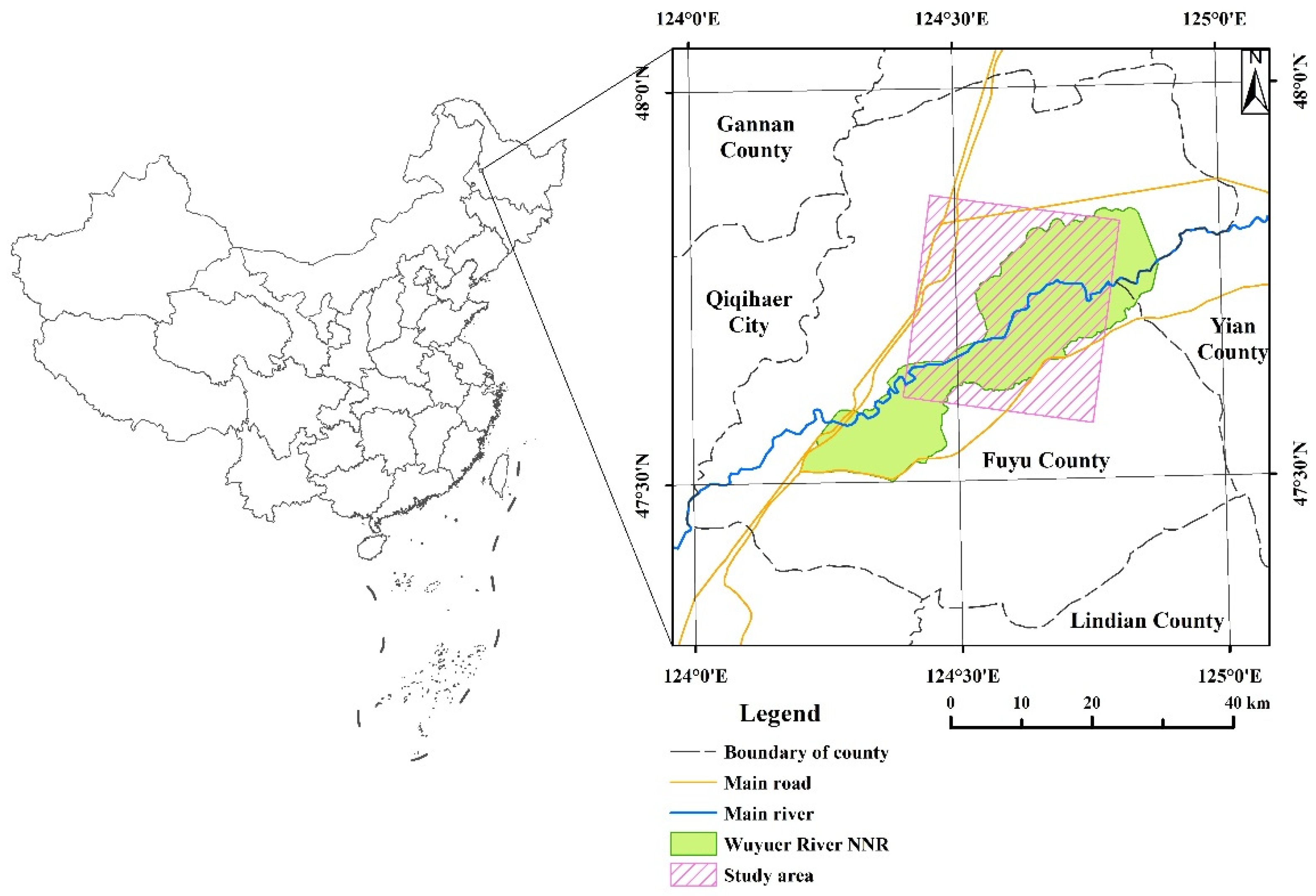
2.1. Study Area

The study area is located at the middle and lower reaches of Wuyuer River in the Northeast Songnen Plain, Heilongjiang Province, China (Latitude: 47°34′ N–47°51′ N, Longitude: 124°23′ E–124°48′ E), covering an area of 782.32 km² (Figure 1). Wuyuer River, which is the second-largest inland river in China, originates from the west of the Lesser Khingan Mountains to the north of Songnen Plain and travels a total length of 587 km [69]. Extensive wetlands have developed due to the low elevation and the poor drainage of the sluggish river. The government reinforces the management of human activities and proposes to establish natural reserves to protect the fragile wetland ecosystems. The Wuyuer River Wetland National Natural Reserve formally established in 2013 has played an important role in nature resources conservation. This region is characterized by a typical semi-humid monsoon climate and four distinct seasons. The annual average temperature ranges 3.2–4.4 °C, and the annual average precipitation approximately ranges 369–440 mm [70]. Marsh; paddy field; and surface water (rivers, lakes, and reservoir) are the primary wetland land cover types in the Wuyuer River Wetland National Natural Reserve. Phragmites australis and Carex (Carex pseudocuraica, Carex meyeriana, Carex enervis, etc.) are the major plant types in the wetland, and some hydrophilous vegetation may also exist [71]. Moreover, our study area also includes the surrounding area of the Wuyuer River Wetland National Natural Reserve that is the main area of frequent human activity in the region, of which the non-wetland types are upland field, meadow, forest, residential area, and road.

2.2. Datasets

2.2.1. Remote Sensing Satellite Imagery

Sentinel-2 and Radarsat-2 remote sensing data were both used for land cover classification over the study area, which can provide visible, infrared, and microwave electromagnetic spectrum information. The Copernicus Sentinel-2 mission provides a global coverage of Earth’s land surface to monitoring the environment condition changes by a constellation of Sentinel-2A and Sentinel-2B. The multispectral instrument contains 13 spectral bands with the central wavelength ranging from 0.443 μm to 2.190 μm (Band 1 (443 nm), Band 2 (490 nm), Band 3 (560 nm), Band 4 (665 nm), Band 5 (705 nm), Band 6 (740 nm), Band 7 (783 nm), Band 8 (842 nm), Band 8A (865 nm), Band 9 (945 nm), Band 10 (1375 nm), Band 11 (1610 nm), and Band 12 (2190 nm)). The Sentinel-2 sensor features three spatial resolutions (10 m, 20 m, and 60 m) on different bands. Level-1C Sentinel-2 TOA products with UTM/WGS84 projection information are freely accessible for global users, which can be downloaded from Sentinel’s Scientific Data Hub (https://scihub.copernicus.eu/, accessed on 9 December 2021).

Radarsat-2 is an advanced commercial C-band (5.405 GHz) SAR satellite that was launched by the Canadian Space Agency (CSA) and MacDonald, Dettwiler and Associates Ltd. (MDA) in December 2007 [33]. The SAR sensor is designed with a multipolarization mode (HH, VV, HV, and VH), which can improve the discrimination among land cover types due to the different sensitivities of each scattering mode to various surface characteristics. Radarsat-2 Fine Quad-Pol images (Single Look Complex, SLC) with a resolution of 4.7 m × 5.1 m and an incidence angle of 45.41° were used for land cover classification in this study [32]. In this study, the Sentinel-2 and Radarsat-2 images were acquired on 9 September 2017 and 27 August 2017, respectively, which were collected in accordance with the dates of the field surveys.

2.2.2. Field Survey Data

The field survey was conducted to collect the field reference samples of different land cover types during September 2017 in the study area. Sentinel-2, Radarsat-2, and high-resolution Google Earth images were used as a reference map to facilitate the collection of ground truth and remote sensing imagery characteristics. In the field investigations, properties of the land cover classes (names, type characteristics, and surrounding description) were recorded in a notebook, and the ground coverage was recorded photographically. The geographical coordinates of the sampling stations were recorded using a Trimble PXRS (Trimble Navigation Inc., Sunnyvale, CA, USA) global positioning system (GPS). During the field survey, a total number of 500 ground truth field plots were collected.

2.3. Image Preprocessing

Sen2cor is a prototype processor that performs Atmospheric Correction (AC, including Cirrus clouds and terrain correction) for Sentinel-2 MSI products. A Level-1C (L1C) Top-of-Atmosphere (TOA) image was converted into an orthoimage Level-2A (L2A) Bottom-of-Atmosphere (BOA) reflectance product by executing the Sen2cor via the windows command line [72]. The generated L2A image was resampled with 10-m spatial resolution for Band 2-Band 8A and Band 11-Band 12 using the Sentinel-2 Toolbox (Sentinel Application Platform, SNAP). The Aerosols Band 1, Water vapor Band 9, and Cirrus Band 10 with 60-m spatial resolution was omitted due to the insignificant information of the ground coverage. The spectral reflectance data extracted from Sentinel-2 L2A resampled imagery was used as variables for the machine learning modeling.

The Radarsat-2 image was preprocessed by using PolSARpro v5.0 software, which was developed by the European Space Agency (ESA) for polarimetric SAR data scientific analysis. This software provided a series of professional data processing procedures, which we implemented on the Radarsat-2 image, including radiation calibration, filtering, and polarimetric decomposition. The original data were converted into backscattering intensity data in dB format by radiometric calibration. A polarimetric coherency (T3) matrix was extracted from the scattering matrices for polarimetric decomposition. A 5 × 5 filtering window was applied to reduce the effects of speckle through the Lee-Sigma filtering method [32]. Several polarimetric decomposition methods were applied to extract the radar polarimetric information.

Finally, in order to unify the geographical spatial coordinate reference of two kinds of satellite imagery, the Sentinel-2 image was used as a reference map to correct the Radarsat-2 image. The geometric correction was carried out by the quadratic polynomial method in ENVI 5.1 software (Exelis Visual Information Solutions, Inc., Boulder, CO, USA). A total of 200 ground control points (GCPs) assured the correction error within one image pixel. The corrected Radarsat-2 image was resampled to 10-m spatial resolution with UTM/WGS84 projection information, which was the same as Sentinel-2.

2.4. Multisource Features Extraction and Selection

2.4.1. Multisource Features Extraction

A large set of multisource features extracted from optical and radar imagery were used as the original feature set. The spectral features were the spectral reflectance of 10 Sentinel-2 MSI bands (Band 2, Band 3, Band 4, Band 5, Band 6, Band 7, Band 8, Band 8A, Band 11, and Band 12). The radar features were extracted using several polarimetric decomposition methods, which were proposed according to the physical scattering mechanisms of ground surface objects [73]. The scattering (S) matrix was acquired from SAR data by measuring the amplitude and phase of the backscattering signal in each pixel, which can be expressed as follows:

$$S=\left[\begin{array}{cc}{S}_{HH}& S_{HV}\\ S_{VH}& S_{VV}\end{array}\right]$$

(1)

where S_HH, S_HV, S_VH, and S_VV represented the complex scattering coefficients of the HH, HV, VH, and VV polarizations, respectively.

A polarimetric coherency (T3) matrix is converted from the S matrix, which can be expressed as follows:

$${\mathrm{T}}_{3\times 3}=\frac{1}{2}\left[\begin{array}{ccc}\langle {\left|S_{HH}+S_{VV}\right|}^2\rangle & \langle \left(S_{HH}+S_{VV}\right){\left(S_{HH}-S_{VV}\right)}^{\ast }\rangle & \langle 2\left(S_{HH}+S_{VV}\right)S_{HV}^{\ast }\rangle \\ \langle \left(S_{HH}-S_{VV}\right){\left(S_{HH}+S_{VV}\right)}^{\ast }\rangle & \langle {\left|S_{HH}-S_{VV}\right|}^2\rangle & \langle 2\left(S_{HH}-S_{VV}\right)S_{HV}^{\ast }\rangle \\ \langle 2S_{HV}{\left(S_{HH}+S_{VV}\right)}^{\ast }\rangle & \langle 2S_{HV}{\left(S_{HH}-S_{VV}\right)}^{\ast }\rangle & \langle 4{\left|S_{HV}\right|}^2\rangle \end{array}\right]$$

(2)

where * denotes the conjugate, |·| denotes the module, and 〈 〉 denotes the temporal scattering matrix and polarimetric coherency or spatial ensemble averaging.

The scattering matrix and polarimetric coherency matrix can be used for extracting polarimetric decomposition features [36,74]. These features can provide the geometrical structure, roughness, and orientation information of different ground targets [32]. Moreover, polarimetric features from different algorithms have different sensitivities to land covers. In this paper, we used the Pauli, Huynen, Barnes, Cloude, Holm, Freeman, Van Zyl, Krogager, H/A/Alpha, and Yamaguchi methods to extract 44 polarimetric decomposition features (

Table 1. List of the polarimetric decomposition features extracted from the Radarsat-2 image using 10 decomposition algorithms.

Decomposition Method	Polarimetric Decomposition Features	Abbreviation	Reference
Pauli	Pauli_a	Pauli_a	Cloude, S.R. [75]
	Pauli_b	Pauli_b
	Pauli_c	Pauli_c
	Pauli_T11	Pauli_T11
	Pauli_T22	Pauli_T22
	Pauli_T33	Pauli_T33
Huynen	Huynen_T11	JRH_T11	Huynen, J.R. [76]
	Huynen_T22	JRH_T22
	Huynen_T33	JRH_T33
Barnes	Barnes_T11	RMB_T11	Barnes, R.M. [77]
	Barnes_T22	RMB_T22
	Barnes_T33	RMB_T33
Cloude	Cloude_T11	SRC_T11	Cloude, S.R. [78]
	Cloude_T22	SRC_T22
	Cloude_T33	SRC_T33
Holm	Holm_T11	WAH_T11	Holm, W.A. [79]
	Holm_T22	WAH_T22
	Holm_T33	WAH_T33
Freeman3	Freeman3_Vol	FRE3_Vol	Freeman, A. [80]
	Freeman3_Odd	FRE3_Odd
	Freeman3_Dbl	FRE3_Dbl
Van Zyl3	Van Zyl3_Vol	VZ3_Vol	Vanzyl, J.J. [81]
	Van Zyl3_Odd	VZ3_Odd
	Van Zyl3_Dbl	VZ3_Dbl
Krogager	Krogager_Kd	KRO_Kd	Krogager, E. [82]
	Krogager_Kh	KRO_Kh
	Krogager_Ks	KRO_Ks
H/A/Alpha	H/A/Alpha_T11	HAA1_T11	Pottier, E. [83]
	H/A/Alpha_T22	HAA1_T22
	H/A/Alpha_T33	HAA1_T33
	H/A/Alpha_Alpha	HAA2_alp
	H/A/Alpha_Anisotropy	HAA2_ani
	H/A/Alpha_Entropy	HAA2_ent
	H/A/Alpha_DERD	HAA3_DERD
	H/A/Alpha_SERD	HAA3_SERD
	H/A/Alpha_RVI	HAA3_RVI
	H/A/Alpha_Polarization asymmetry	HAA3_PA
	H/A/Alpha_Polarization fraction	HAA3_PF
	H/A/Alpha_Pedestal height	HAA3_PH
	H/A/Alpha_Shannon entropy	HAA3_SE
Yamaguchi4	Yamaguchi4_Vol	YAM4_Vol	Yamaguchi, Y. [84]
	Yamaguchi4_Odd	YAM4_Odd
	Yamaguchi4_Dbl	YAM4_Dbl
	Yamaguchi4_Hlx	YAM4_Hlx

).

2.4.2. Multisource Features Selection Method

A large set of multisource features was extracted to comprehensively obtain ground surface information. However, some features may provide redundant or noise information, which can confuse the data mining procedure of machine learning algorithms. Therefore, it is necessary to use some efficient methods to select different features that are sensitive to various land cover types and provide significant information.

The ReliefF algorithm is a widely used filtering feature selection algorithm, which can solve multiclass problems [85]. This algorithm is considered as one of the most successful feature selection algorithms due to its high efficiency and unrestricted data types. The main principle of ReliefF algorithm is that, given a dataset D, a sample x is randomly selected from it, and the k-nearest samples H(x) and k-nearest samples M(x) are, respectively, searched from the same class and different class with sample x. The sum of the distances between sample x and the k-nearest samples is calculated, and the weight values of the features are updated according to the distances. The feature weight value is updated as follows:

$$W_f^i=W_f^{i-1}+{\displaystyle \sum _{C\ne class(x)}\frac{\frac{p(x)}{1-p(class(x))}{\displaystyle \sum _{j=1}^{k}diff(f,x,M(x))}}{m\times k}-{\displaystyle \sum _{j=1}^k\frac{diff(f,x,H(x))}{m\times k}}}$$

(3)

where diff(·) is the distance of different samples on feature f, p(x) is the probability of the class, H(x) and M(x) are k-nearest samples searched from same class and different class, respectively, m is the number of iterations, k is the number of the nearest samples, and i is a randomly selected sample.

The random forest (RF) algorithm is an ensemble learning algorithm based on multiple classification and regression tree (CART) integration [86]. The algorithm uses bootstrap sampling technology to generate multiple training sets from the original data set to train each CART. During the construction of a CART, each node is split using the features and threshold that yield the smallest Gini coefficient. The Gini coefficient can be defined as follows:

$$Gini(D)=1-{{\displaystyle \sum _{i=1}^m\left(\frac{D_{\mathrm{i}}}{D}\right)}}^2$$

(4)

where D is the number of data samples, m is the number of input features, and D_i represents the number of samples for ith feature.

When the RF algorithm randomly shuffles the value of a feature variable, the validation accuracy will be influenced. The greater the decrease in validation accuracy, the higher the importance of the feature variable. Thus, RF provides variable importance estimations for the qualitative analysis of variable contributions, which has an outstanding ability to screen feature information. The variable importance can be calculated as Equation (5):

$$V(X_j)=(Acc-Ac{c}_j)/Acc$$

(5)

where Acc represents the validation accuracy, Acc_j represents the validation accuracy after shuffling the jth feature X_j, and V(X_j) is the importance of feature X_j.

In this paper, a hybrid feature selection method (ReliefF-RF) was proposed to combine the advantages of two feature selection methods. In the first step, the weight values of total extracted features were calculated by the ReliefF method. The features with weight values above 0.01 were selected into the initial optimal feature set. The features that had a low correlational relationship with different land cover types were effectively removed. In the second step, the feature set optimized by ReliefF was put into the RF algorithm, and the feature importance was calculated according to the validation accuracy. The features were rearranged in descending order of importance. In order to filter the features that have limited potential for increasing the classification accuracy, one feature was added into the RF model for training per iteration, and the overall accuracy was calculated at the same time. The iteration stopped until all the features were added into the model. The features were determined as the final optimal feature set when the accuracy tends to converge.

2.5. Object-Based gcForest (OGCF) Method

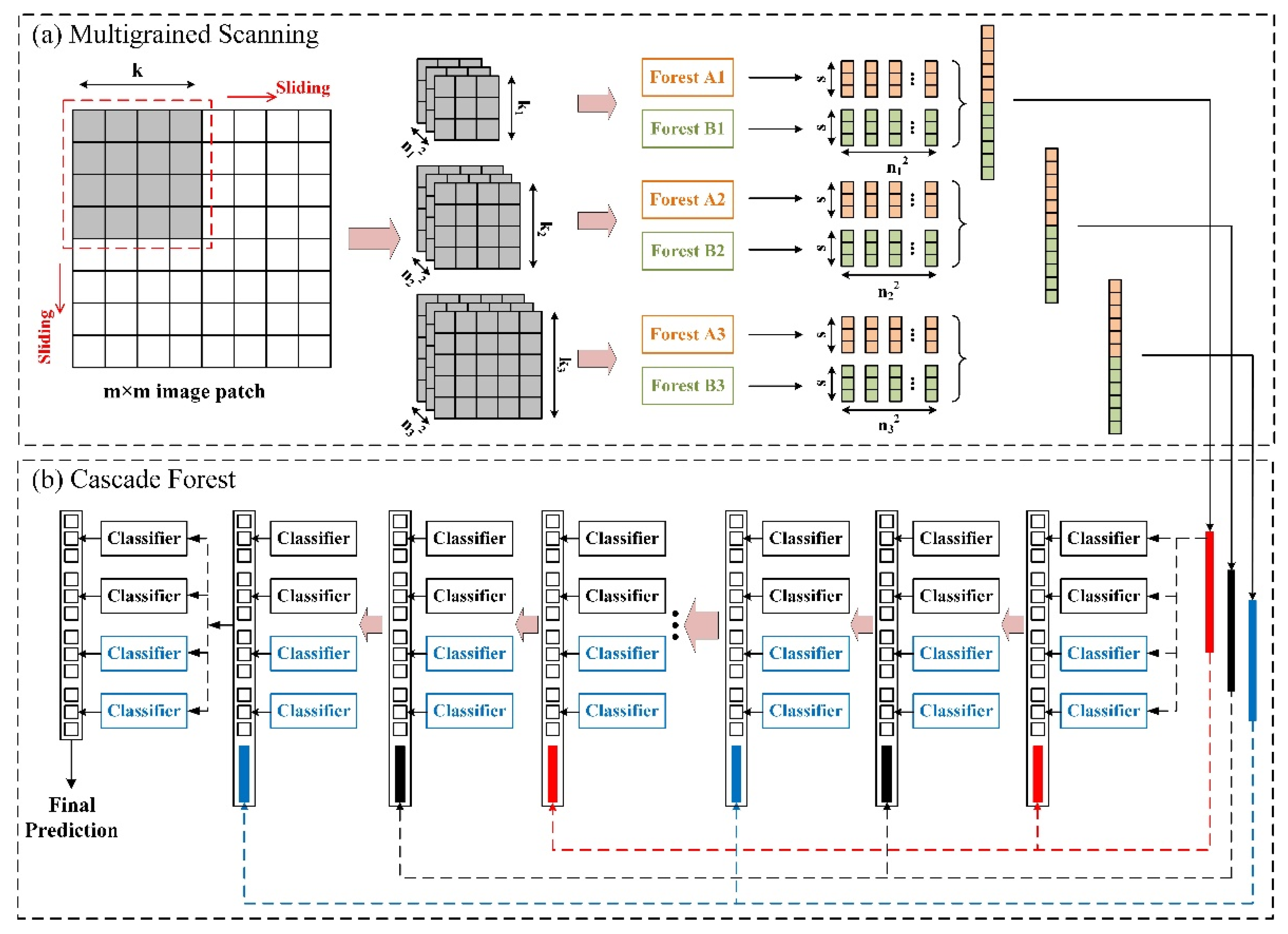
2.5.1. Multigrained Cascade Forest

Multigrained cascade forest (gcForest) is a potential ensemble approach that consists of many base estimators to generate a cascade forest, which was proposed by Zhou’s research [61]. The cascade forest is a deep and layer-by-layer processing structure that is similar to the multilayer neural network structure of deep neural networks (DNN) [87]. Besides the part of cascade forest, multigrained scanning is a special part of gcForest to use for producing new features from the raw image features by sliding windows. Furthermore, as pointed out in Zhou’s research, the gcForest method with fewer hyperparameters is more efficient and performs excellent even on small-scale data [61].

As illustrated in Figure 2a, sliding windows are used to scan the input image patches, which is called multigrained scanning. Suppose the size of input image patches is m × m, then the k × k sliding window for scanning will produce n² feature images, in which n can be computed as in Equation (6). Each base classifier, such as random forest and extra tree [88], produced n² s-dimensional class vectors by using n² feature images. In practice, these class vectors are the classification probability. The class vectors are concatenated as transformed features and then input into the cascade forest. The procedure of multigrained scanning enriches the features and retains the spatial information, which enhances the representation ability of cascade forest. In this paper, we used multiscale sliding windows to increase the feature diversity, with three window sizes applied to scan the image patches.

$$n=\frac{m-k}{d}+1$$

(6)

where m and k represent the size of input image patches and sliding windows, respectively, and d is the step size of the sliding windows.

As illustrated in Figure 2b, cascade forest employs a layer-by-layer structure. Each layer of the cascade structure is an ensemble classifier that consists of several different base classifiers [89]. In this paper, we employed four classifiers, random forest, extra tree, extreme gradient boosting, and logistic regression, as the base classifier [90]. The transformed features generated by multigrained scanning are input into the first layer of cascade forest, and the ensemble classifiers obtain the classification probability as the output class vectors. These class vectors concatenated with transformed features as new features are input into the next layer. Similarly, the current layer uses both of the output class vectors from the previous layer and transformed features from multigrained scanning as the input features for training. Furthermore, due to the use of multiscale sliding window to scan image patches, the transformed features have three sizes, and each layer chooses one size to train the classifiers.

To reduce the risk of overfitting, the class vectors produced by each classier are generated by k-fold cross-validation. After expanding a new layer, the whole cascade forest will be estimated on the validation data, and the training procedure will terminate if the performance has no significant improvement. Therefore, the cascade forest is able to adaptively determine the number of layers such that the model complexity can be automatically adjust.

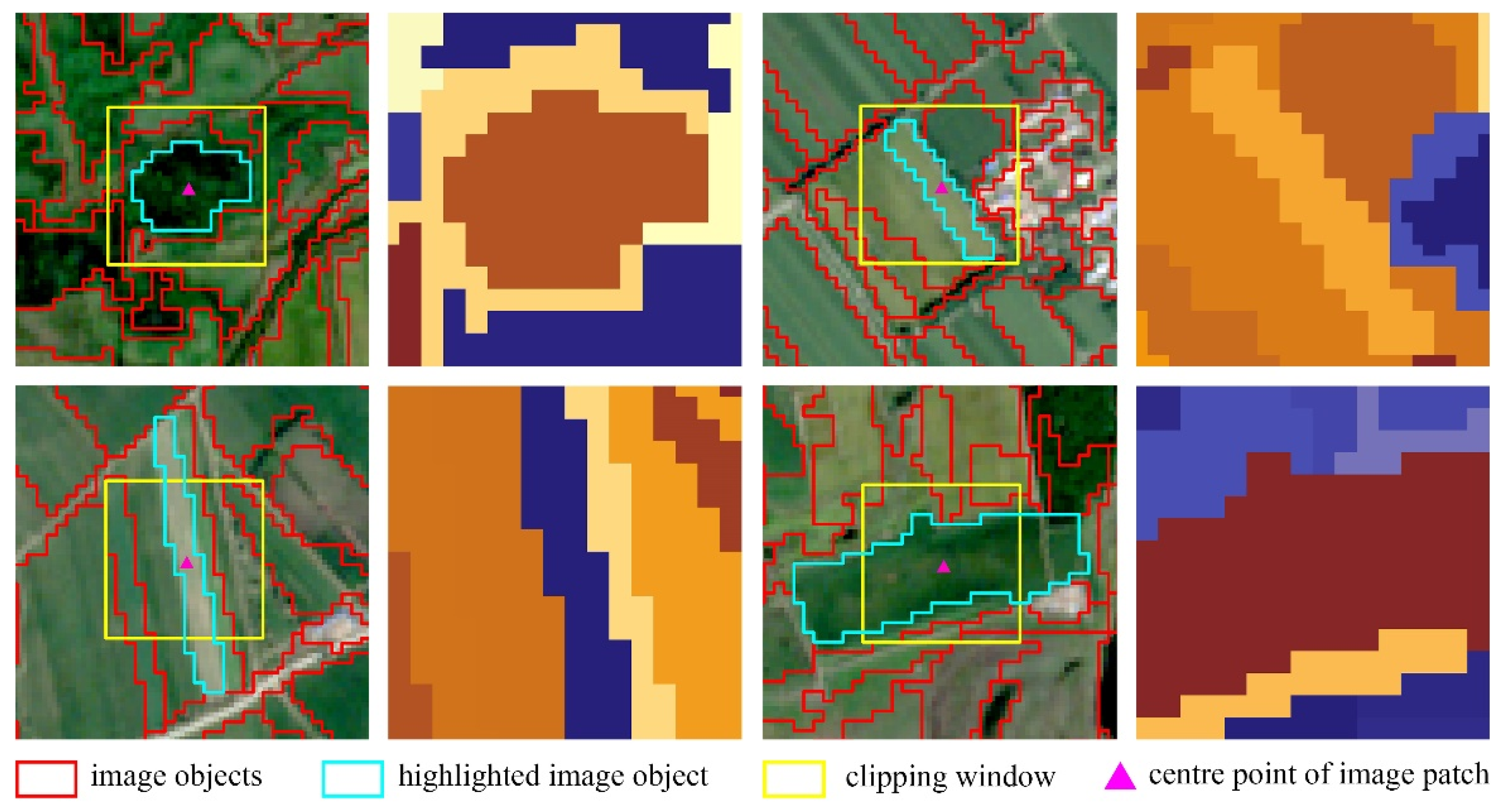
2.5.2. Image Patches Generation with Segmented Object

An object-based gcForest (OGCF) method is proposed for wetland classification, in which the labeled image patches were represented by objects derived from image segmentation. Image segmentation is carried out using the commonly used multiscale segmentation technology via eCognition Developer software (Trimble Inc., Sunnyvale, CA, USA). This algorithm is based on bottom-up region merging of pixels to minimize the heterogeneity of the segmented objects. The main parameters include segmentation scale, spectral heterogeneity, and shape heterogeneity. After several experiments, the segmentation scale, shape, and compactness parameters are set as 60, 0.5, and 0.8, respectively. The final image objects can distinguish different land cover classes in adjacent positions, and the number of objects is moderate. Then, all the image objects are converted into vector polygons in a shapefile using ArcGIS 10.3 software (ESRI Inc., Redlands, CA, USA). The center point of the object that is automatically generated from one polygon is taken as the center to generate an image patch with an appropriate window size (Figure 3). We set several different clipping window sizes (16 × 16, 20 × 20, 24 × 24, 28 × 28, 32 × 32, 36 × 36, 40 × 40, 44 × 44, and 48 × 48) of the image patches and compare them to find which one is the most appropriate. A total 22,807 image patches are generated for the whole remote sensing image. The generated image patches contain the spectral information of the objects and the spatial information of the adjacent object, which are helpful to improve the ability of the model to distinguish different classes.

2.6. Accuracy Assessment

The widely used confusion matrix is applied to assess the classification accuracy. Several evaluation indicators that are calculated from the confusion matrix can be used to comprehensively assess the classification results, including the overall accuracy (OA), kappa coefficient, user’s accuracy (UA), and producer’s accuracy (PA). The OA represents the total proportion of correctly classified. The Kappa coefficient reflects the agreement between classification results and actual reference data [21,91]. The UA describes the proportion of correctly classified in the classification result of per class. The PA describes the proportion of correctly classified in the actual reference sites of per class [91]. A total number of 750 image patches were randomly selected for classification, of which 564 image patches were used for model calibration, and 186 image patches were employed to search the optimal hyperparameters of classifiers for model validation. Furthermore, a total of 500 truth field plots were used to verify the results of the classification.

Table 2. Number of collected samples for the land cover classes over the study area.

Class Code	Land Cover Classes		Number of Samples
			Calibration	Validation	Test
C1	Wetland	Carex marsh	78	26	50
C2		Phragmites marsh	52	17	40
C3		Paddy field	119	39	81
C4		Surface water	85	29	87
C5	Non-wetland	Residential area	67	22	52
C6		Road	15	5	41
C7		Upland field	95	31	80
C8		Forest	6	2	22
C9		Meadow	47	15	47
Total			564	186	500

shows the sample number of each land use type in the calibration, validation, and test datasets.

3. Results

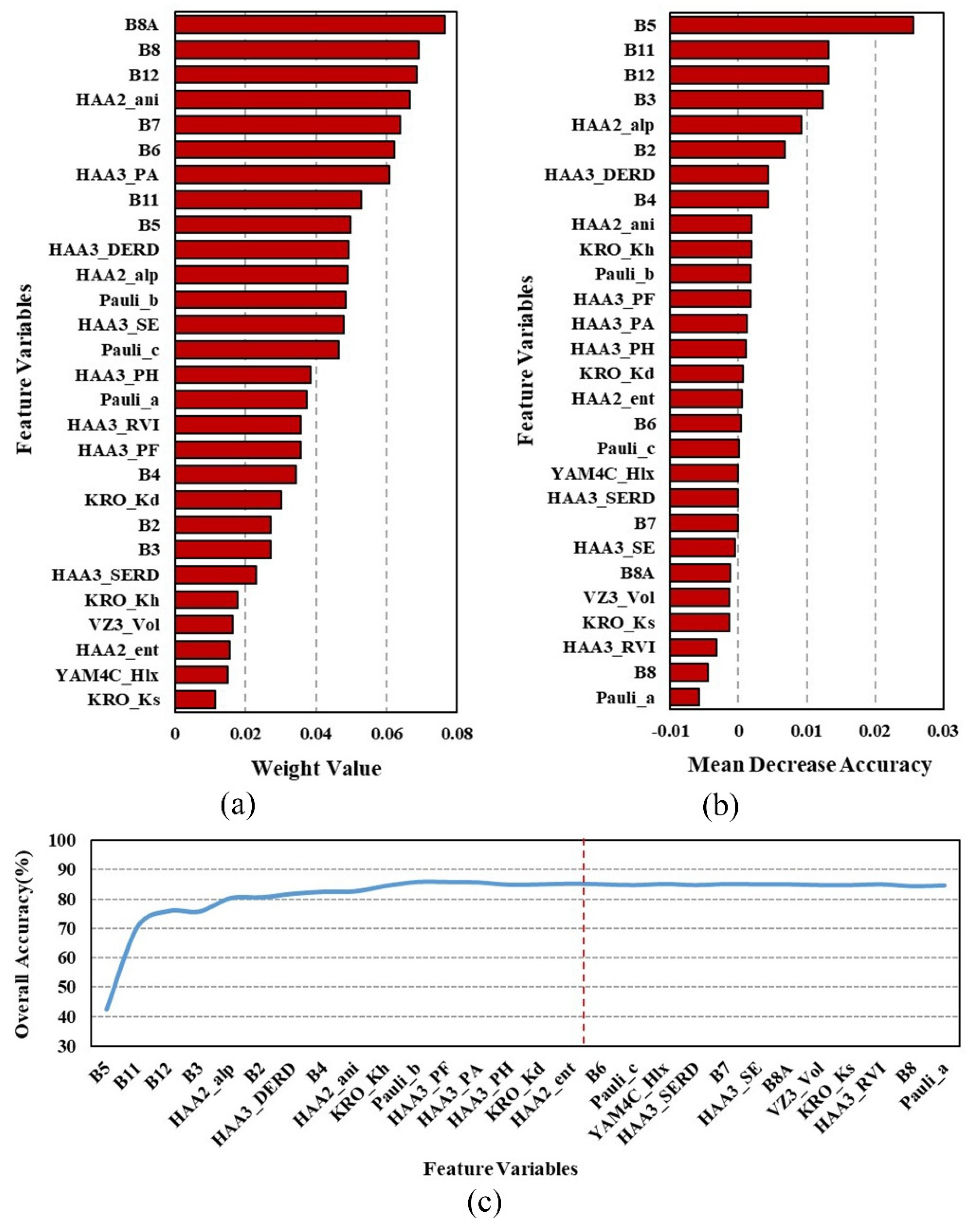
3.1. Multisource Features Importance and Feature Set Optimization

The hybrid feature selection algorithm (ReliefF-RF) was proposed to optimize the feature set with 54 multisource features according to the ranking criterion of ReliefF and RF. As shown in Figure 4a, the number of features selected by the ReliefF method was 28, of which the number of spectral features and polarimetric decomposition features was 10 and 18, respectively. The features with higher weight values were more capable of distinguishing the samples. B8A has the highest weight value of 0.076 among the spectral features, while the KRO_Ks derived from the Krogager decomposition had the lowest weight value of 0.011. Among all of the polarimetric decomposition features, the feature variables obtained by Pauli decomposition, H/A/Alpha decomposition, and Krogager decomposition were selected more frequently.

Though about half of the features were filtered by the ReliefF method, the 28 features were also slightly large in terms of complexity and efficiency in the OGCF model. Some features might play a small role in the classification accuracy increase. RF was employed to further select from the 28 feature variables obtained by ReliefF. Figure 4b shows the feature importance values derived from the validation accuracy of RF in descending order. The higher the importance fractions produced, the more important the feature was. B5 exhibited the highest importance fraction among the spectral features, with the value of 0.026. In terms of the polarimetric decomposition features, HAA2_alp had the highest importance value of 0.009. Figure 4c shows the overall accuracy of the RF method in each iteration. The overall accuracy greatly improved when 11 features with high importance fractions were used in RF. The accuracy reached the highest value of 85.73% and increased 43.20% than using B5 alone in the first iteration. After that, the overall accuracy tended to converge when the number increased to 16. After the 16th feature was added, the accuracy slightly decreased by about 0.70%. Therefore, the 16 features were selected as the final optimized feature set used for wetland land cover classification, including six spectral features (B2, B3, B4, B5, B11, and B12) and 10 polarimetric decomposition features (HAA2_alp, HAA2_ani, HAA2_ent, HAA3_PA, HAA3_PF, HAA3_PH, HAA3_DERD, KRO_Kd, KRO_Kh, and Pauli_b).

3.2. Hyper-Parameters Optimization of OGCF Method

3.2.1. Size of Sliding Window and Image Patch

The sizes of image patch and sliding window jointly affected the generation of features during the multigrained scanning, which was highly significant for the quality of information extraction, model complexity, and model efficiency. We conducted several experiments to investigate the comprehensive influence of sliding window size and image patch size on the overall accuracy and time consumption.

Table 3. Overall accuracy and time consumption using different combinations of image patch size and sliding window size.

Image Patch Size	Sliding Window Size
	8 × 8/12 × 12/16 × 16		12 × 12/18 × 18/24 × 24		16 × 16/24 × 24/32 × 32		20 × 20/30 × 30/40 × 40
	OA (%)	Time (s)	OA (%)	Time (s)	OA (%)	Time (s)	OA (%)	Time (s)
16 × 16	83.86	178
20 × 20	85.81	324
24 × 24	84.22	613	82.62	224
28 × 28	82.80	985	83.51	423
32 × 32	81.74	1351	84.92	702	86.17	489
36 × 36	82.62	1875	82.80	1156	85.28	937
40 × 40	79.43	2521	81.03	1715	84.75	1243	85.46	934
44 × 44	80.49	3128	80.14	2304	82.98	1666	84.22	1347
48 × 48	80.32	3353	78.90	2901	80.49	2365	83.86	1972

shows the OA in the validation set and the time consumption when the OGCF model used different combinations of image patch size and sliding window size. As presented in Table 3, when smaller sliding window sizes (8 × 8/12 × 12/16 × 16 and 12 × 12/18 × 18/24 × 24) were selected, with the image patch size increasing, the OA gradually improved and reached the highest values of 85.81% with a 20 × 20 image patch size and 84.92% with a 32 × 32 image patch size, respectively. After that, the OA decreased; meanwhile, the time consumption increased significantly. When using larger sliding window sizes (16 × 16/24 × 24/32 × 32 and 20 × 20/30 × 30/40 × 40), the OA reached the highest values of 86.17% with a 32 × 32 image patch size and 85.46% with a 40 × 40 image patch size, respectively. The OA decreased gradually when the image patch size increased. When using a fixed image patch size, with the sliding window size increasing, the OA increased, and the time consumption decreased. Based on integration of the upwards experiments, we selected the combination of a 32 × 32 image patch size and a 16 × 16/24 × 24/32 × 32 sliding window size with the OA value of 86.17% and the time consumption of 489 s as the optimal combination in this study.

3.2.2. Base Classifiers

The base classifiers employed in cascade forest can theoretically be any type that ensured model diversity. Further, the number of base classifiers was another important hyperparameter that influenced the model performance. As shown in

Table 4. Overall accuracy and time consumption using different number of base classifiers. E1–E6 represent the codes of the experimental groups.

Classifier Type	Number of Base Classifiers
	E1	E2	E3	E4	E5	E6
RF	1	1	1	2	2	2
ET	1	1	1	1	2	2
XGBoost	0	1	1	1	1	2
LR	0	0	1	1	1	2
Overall Accuracy (%)	76.95	84.75	85.99	82.97	83.15	84.04
Time(s)	295	423	502	505	608	735

, we chose four kinds of base classifiers, including random forest (RF), extra trees (ET), extreme gradient boosting (XGBoost), and the logistic regression (LR) method. The combinations of image patch size and sliding window size in the multigrained scanning step were, respectively, set to 32 × 32 and 16 × 16/24 × 24/32 × 32, which achieved the highest OA in the previous experiment. Among all the experimental groups, the OA value significantly improved by using four kinds of base classifiers. The ensemble method with two classifiers (random forest and extra tree) performed poorly, with the lowest OA value of 76.95%. The OA value significantly improved with an increase in the kinds of base classifiers, and the method that consisted of four different base classifiers produced higher OA values above 85.99% (E1–E3). According to experimental groups 4–6 (E4–E6), the number of each type of classifier was imbalanced and produced lower OA values (E4, OA = 82.97%; E5, OA = 83.15%). In addition, the running time was significantly increased with the base classifier number increasing.

3.3. Classification Results

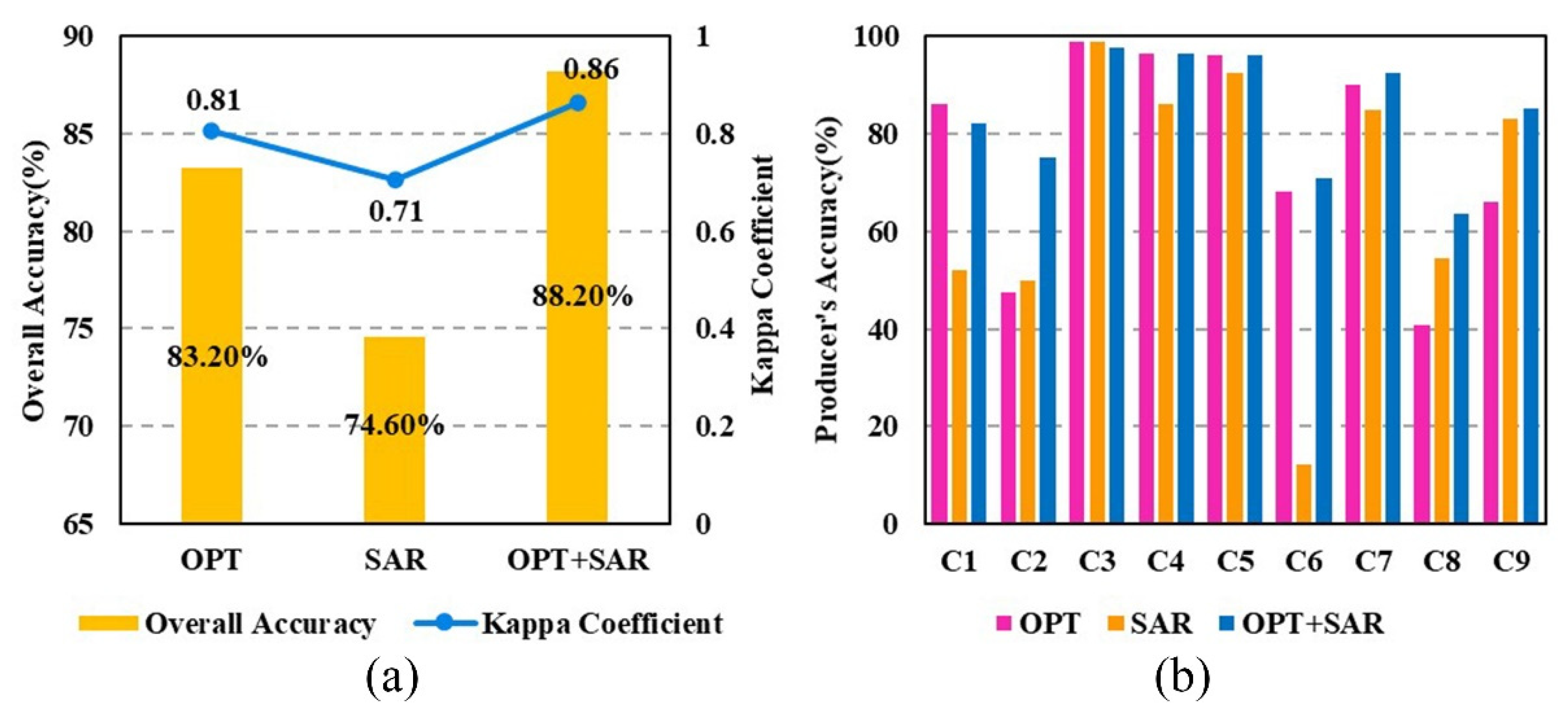
3.3.1. Accuracy Assessment of OGCF Model with Different Feature Sets

Figure 5 shows the overall accuracy, kappa coefficient, and producer’s accuracy calculated from the confusion matrix, which was obtained from the classification results of the OGCF model with different feature sets. As shown in Figure 5a, when using individual types of features for classification, the model with spectral features outperformed the model with polarimetric decomposition features (OPT: OA = 83.20%, kappa = 0.81; SAR: OA = 74.60%, kappa = 0.71). The method with multisource features produced the highest classification accuracy, with the OA value of 88.20% and kappa coefficient of 0.86.

According to Figure 5b, the OGCF model with three feature sets yielded different PA values of the various land cover classes. The highest PA of four classes (residential area, upland field, paddy field, and surface water) were close to 100%. The accuracy insignificantly improved when using different feature sets. The PA value of upland field and surface water increased by up to 92.50% and 96.55%, respectively, when using multisource features rather than optical or radar features alone, while the PA value of the residential area increased to 96.15%. The model with individual spectral features produced the lower PA for forest and meadow with the values of 40.91% and 65.96%, respectively. The model with individual polarimetric decomposition features produced the lower PA for Carex marsh and road with the values of 52.00% and 12.20%, respectively. The accuracy of the phragmites marsh was lower when using individual features (OPT, PA = 47.50%; SAR, PA = 50.00%). However, the PA of all of these classes significantly improved using multisource features. The accuracy of the phragmites marsh improved most obviously by 27.50% and 25.00%, respectively, compared with using optical and radar features alone, followed by forest (22.73% and 9.09%) and meadow (19.15% and 2.13%).

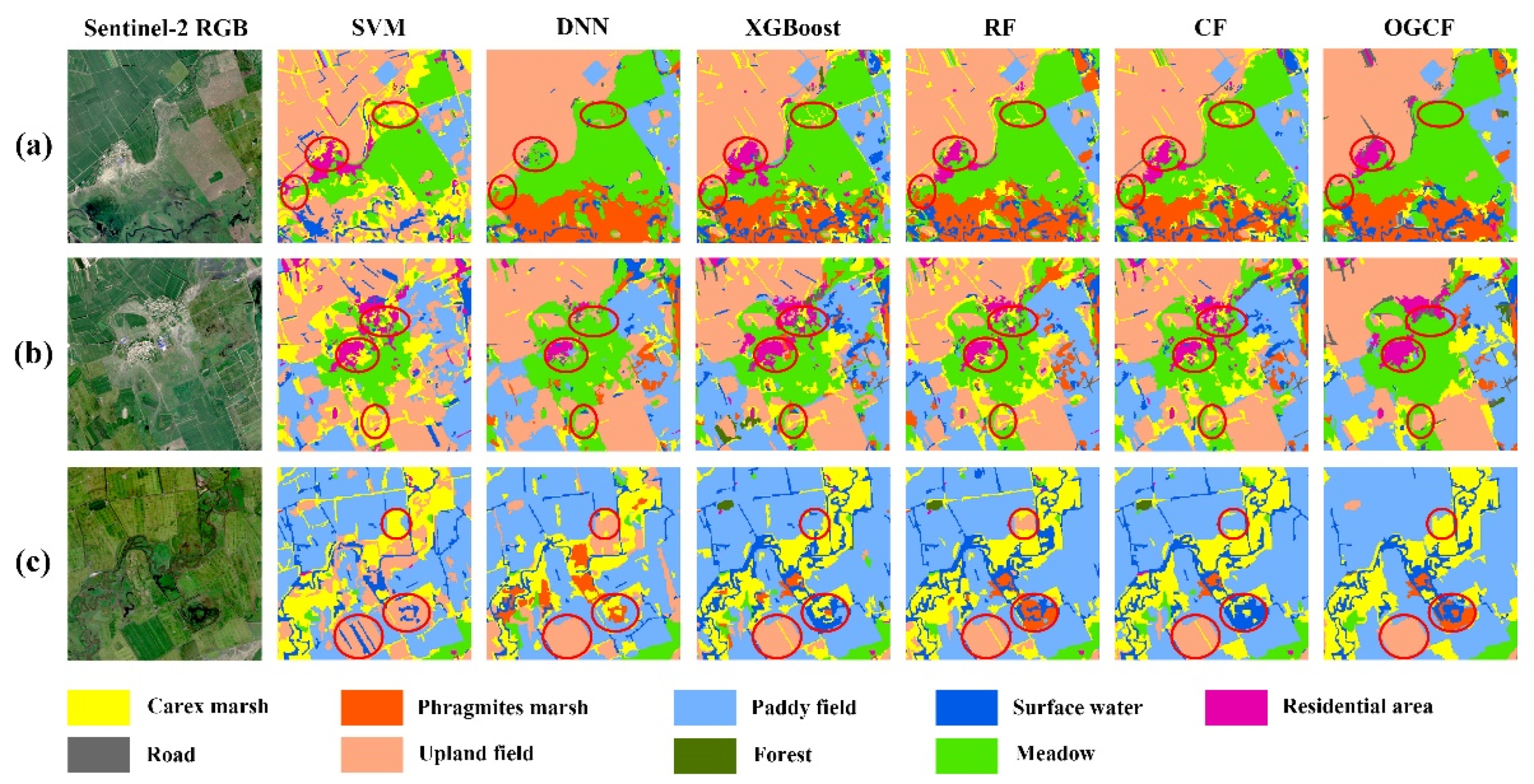
3.3.2. The OGCF Model Compared with Different Classification Methods

Figure 6 shows the overall accuracy, kappa coefficient, and producer’s accuracy calculated from the confusion matrix, which was obtained from the classification results of several classification methods by using a hybrid feature set (including spectral features and polarimetric decomposition features). The compared methods included support vector machine (SVM), deep neural network (DNN), extreme gradient boosting (XGBoost), random forest (RF), cascade forest (CF), and object-based gcForest (OGCF). SVM and DNN yielded lower classification accuracies (SVM: OA = 70.00%, kappa = 0.65; DNN: OA = 78.60%, kappa = 0.75). The classification accuracy obviously increased when using ensemble methods, including XGBoost, RF, and CF (XGBoost: OA = 83.40%, kappa = 0.81; RF: OA = 84.80%, kappa = 0.82; CF: OA = 85.60%, kappa = 0.83), and the OGCF achieved the highest classification accuracy with the OA value of 88.20% and kappa coefficient of 0.86 (Figure 6a).

As illustrated in Figure 6b, the classification accuracy of each land cover class was different when using different classification methods. The PA values of the upland field and paddy field were similar and relatively high among the six methods. The SVM produced the low PA for forest, meadow, phragmites marsh, and road with the values of 22.73%, 61.70%, 12.50% and 12.20%, respectively. The DNN produced low PA for forest, Carex marsh, and road with the values of 27.27%, 54.00%, and 48.18%, respectively. The XGBoost and RF performed well and yielded higher PA for most of land cover classes. A few land cover classes had low PA, such as Carex marsh with the value of 66.00% in XGBoost and road with the value of 46.34% in RF. The CF produced a comparatively high PA for each land cover, except for the phragmites marsh. By contrast, the PA value of the phragmites marsh was significantly improved by 17.50% by using the OGCF method. Comparing with other methods, OGCF produced the highest PA for the residential area, forest, Carex marsh, and surface water with the values of 96.15%, 63.64%, 82.00%, and 96.55%, respectively. As for the other five land cover classes, OGCF also produced good results. The accuracy of the wetland classes ranged from 75.00% to 97.53%.

Furthermore, for visual assessment, three subregions in the study area are presented in Figure 7, and red circles are used to mark the details of classification maps of different classification methods. As shown in Figure 7, OGCF achieved the most accurate results and had the fewest scattered objects in the classification map. Some classes, such as meadow, field, phragmites marsh, and Carex marsh, had similar textures, geometrical structures, and adjacent spatial patterns. These easily misclassified classes were identified better by using the OGCF method, and the class boundaries were smoother and more precise. In terms of the other classification methods, the meadow was partially misclassified as the Carex marsh and the upland field mistakenly mixed Carex marsh by XGBoost, RF, and CF. Moreover, XGBoost and CF could not distinguish phragmites marsh from surface water well. SVM classified worst, which seriously misclassified phragmites marsh as upland field and misclassified meadow as Carex marsh. For the other classes, all of the six methods had satisfactory results for the upland field and paddy field. The residential area was identified better by the OGCF model, whereas the residential area class patches were dispersal, boundaries were blurred, and the accuracy results were poorer in other five classification maps.

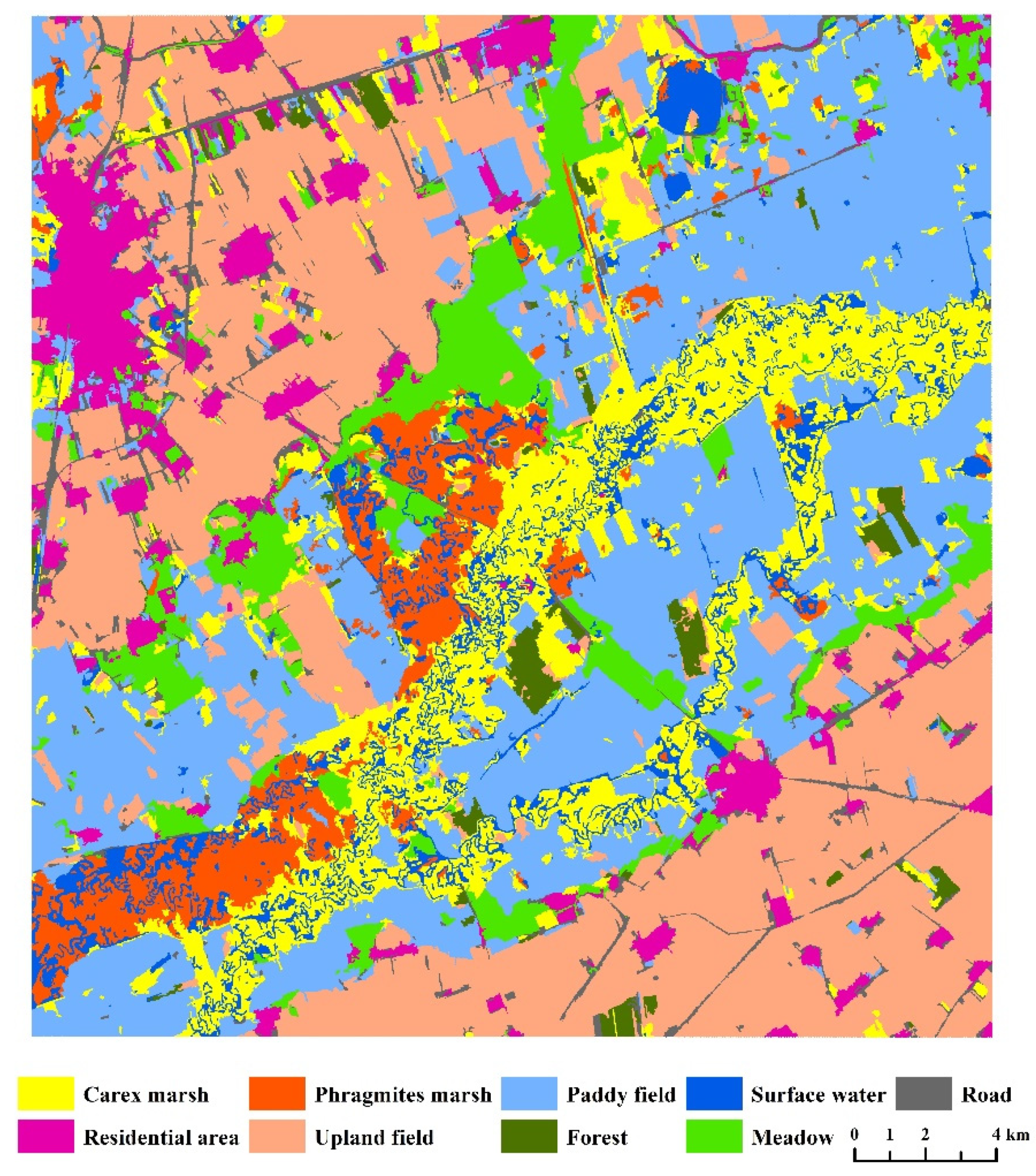
3.3.3. Classification Result of OGCF Method

The classification result of the whole study area obtained by the OGCF method is presented in Figure 8, and the producer’s accuracy, user’s accuracy, overall accuracy, and kappa coefficient calculated from confusion matrix are provided in

Table 5. The confusion matrix of the OGCF classification results. The matrix shows the number of verification points, producer’s accuracy, user’s accuracy, overall accuracy, and kappa coefficient. C1–C9 are the class codes that represent different land cover classes (see Table 2).

	C1	C2	C3	C4	C5	C6	C7	C8	C9	UA (%)
C1	41	3	1	3	0	0	2	5	5	69.49
C2	0	30	0	1	0	0	0	0	1	93.75
C3	5	0	79	0	0	3	3	0	0	87.78
C4	1	6	0	84	0	0	0	0	0	92.31
C5	0	0	1	0	50	5	0	0	1	87.72
C6	0	0	0	0	1	29	0	0	0	96.67
C7	0	0	0	0	0	3	74	3	0	92.50
C8	0	0	0	0	0	0	1	14	0	93.33
C9	3	1	0	0	1	1	0	0	40	86.96
PA (%)	82.00	75.00	97.53	96.55	96.15	70.73	92.50	63.64	85.11
Overall Accuracy = 88.20%
Kappa Coefficient = 0.86

. As shown in Figure 8, the classification map exhibited smooth results, which remained spatial distribution characteristics and accurate boundaries of land cover classes. The isolate objects were effectively removed. As shown in Table 5, the OA of the OGCF method was 88.20%, and the kappa coefficient was 0.86. For wetland classes, the paddy field and surface water achieved the highest classification accuracy with PA values of 97.53% and 96.55%, respectively, and UA values of 87.78% and 92.31%, respectively. Carex marsh and phragmites marsh had PA values of 82.00% and 75.00%, respectively, and UA values of 69.49% and 93.78%, respectively. Carex marsh was mainly misclassified into meadow and paddy field, while phragmites marsh was mainly misclassified into Carex marsh and surface water. For non-wetland classes, the residential area and upland field achieved the highest classification accuracy with PA values of 96.15% and 92.50%, respectively, and UA values of 87.72% and 92.50%, respectively. The PA of meadow was 85.11%, and meadow was mainly misclassified in Carex marsh. The PA values of forest and road were comparatively low with values of 63.64% and 70.73%, respectively. Forest was mainly misclassified into upland field and Carex marsh, while road was misclassified with many other classes.

4. Discussion

4.1. Multisource Features Analysis

A large set of multisource features were extracted from optical and radar data (Sentinel-2 and Radarsat-2 imagery) and then selected by using a proposed hybrid method (ReliefF-RF), which combined the advantages of the ReliefF and RF methods. In terms of the spectral features, the results showed that B5, B11, B12, B3, B2, and B4 were selected and sorted in descending order of importance. B5 was the red edge band from the Sentinel-2 satellite sensor, which was used to identify the vegetation characteristics. B11 and B12 were shortwave infrared bands, of which the surface water body reflectivity was close to 0 and also had an effect on plants. Regarding the marsh wetland, the fine wetland classes were determined by the dominated vegetation types, such as phragmites marsh and Carex marsh. The constructed wetland was a paddy field with a high soil moisture content. Moreover, some non-wetland classes, upland field, forest, and meadow, also had different vegetation characteristics. The selected spectral bands in the red edge and infrared can efficiently reflect the characteristics of vegetation and water. B3, B2, and B4 were green, blue, and red bands that can reflect the visible spectral information of different classes, such as road and residential area. Due to the prominent differences of the selected spectral features, OGCF effectively extracted characteristic information and produced good classification results with an overall accuracy of 83.20%.

In terms of the polarimetric decomposition features, the results showed that HAA2_alp, HAA3_DERD, HAA2_ani, KRO_Kh, Pauli_b, HAA3_PF, HAA3_PA, HAA3_PH, KRO_Kd, and HAA2_ent were selected and sorted in descending order of importance. The H/A/Alpha decomposition method had obvious advantages in feature extraction, which made full use of the expressed information obtained from the eigenvalues of the coherence matrix. This algorithm identified the dominant scattering mechanism via extraction of the largest eigenvalue, which can provide physical interpretation [32,37]. The scattering angle alpha (HAA2_alp) reflected the dominant scattering mechanism of different classes, such as surface scattering (surface water), double-bounce scattering (buildings in the residential area), and volume scattering (the surface objects covered vegetation). Moreover, the entropy of polarized wave states in random media (HAA2_ent) can reflect the depolarizing performance and polarization anisotropy (HAA2_ani) was supplementary of polarization entropy, which described the minor scattering mechanism. The combination of scattering angle alpha, polarization entropy, and polarization anisotropy can more accurately identify classes [78,92]. Other H/A/Alpha polarimetric features were newly derived from the coherence matrix, showing that DERE (HAA3_DERD) can describe the surface roughness of ground objects, and the polarization fraction (HAA3_PF), polarization asymmetry (HAA3_PA), and pedestal height (HAA3_PH) can reflect randomness and depolarization characteristics [93]. The Pauli and Krogager methods were polarization coherent decomposition methods, which aimed at separating the target returns into an averaged singled target, and the target scattering matrix was decomposed into three components. Coefficient b (Pauli_b) for Pauli reflected the contribution of double-bounce scattering, and components Kd (KRO_Kd) and Kh (KRO_Kh) described that scattering was caused by oriented di-plane and a right or left wound helix [82]. Therefore, it had advantages in using these polarimetric decomposition features to distinguish similar wetland classes due to the different physical scattering mechanisms, just as the results showed that similar wetland classes, such as Carex marsh and phragmite marsh, were more accurately distinguished when adding polarimetric features. The dominant vegetation of wetlands with different heights, shapes, structures, and growth environments may cause different electromagnetic wave scattering. The classification accuracy obviously improved due to the effective information extraction of scattering features using the OGCF method. Moreover, the scattering characteristics also helped to identify non-wetland classes, such as forest and meadow, which both covered vegetation with different surface roughness.

The final optimal feature set that was selected by the hybrid method (ReliefF-RF) can reflect the actual physical characteristics and had certain universality that may be appropriate for different classifiers. ReliefF efficiently filtered out many of the features according to the correlations between the features and land cover classes. Besides the correlation relationship, features were further selected using the variables’ importance in RF, which can reflect the contribution to classification accuracy. In addition, the improvement of classification accuracy was also attributed to the utilization of multisource features. The land cover classes may easily be misclassified by using spectral features alone due to the similar spectrum with different objects. The classification accuracy may be also lower by using polarimetric features alone due to the speckle noise of SAR data. Speckle noise is caused by the coherent superposition of the scattering echo signals and may hardly be completely remove, even when executing speckle filtering. It may seriously influence the extraction of polarimetric decomposition features. Therefore, the combined utilization of spectral and polarimetric decomposition features can significantly improve the classification accuracy of wetlands and its surrounding non-wetland ground objects.

4.2. Object-Based gcForest Method

4.2.1. Hyperparameter Optimization

The image patch size for input samples, the sliding window size for multigrained scanning, and the base classifier for cascade forest were the crucial hyperparameters for the OGCF model. The size of the image patch and sliding window jointly influenced the classification accuracy, model complexity, and computational efficiency. The image patch size determined the retention of segmented object. Too small of a size could not contain complete class characteristics and spatial information with adjacent classes, whereas too large of a size will produce a lot of useless background information and reduce the computing efficiency. Similarly, the sliding window size for multigrained scanning directly influences the size and number of feature images, which can enrich the input features from raw image features. Small sliding window sizes cause the extracted feature images to be too scattered and the spatial characteristics to be incoherent. A large number of feature samples unrelated to the target class will be generated, which may become noise data and affect the classification accuracy. However, a large sliding window may lead to generating fewer feature images. It causes feature images to be similar and provides redundant class characteristics and spatial information. Thus, the features of image patch cannot be fully extracted. Furthermore, the size of the image patch and sliding window directly influence the computational complexity and efficiency of a model.

In terms of the base classifier of cascade forest, the OGCF model, which combined four base classifier types, can enhance the diversity of classifiers and combine the advantages of various classifiers; thus, the generalization ability was effectively improved. The experimental results indicated that the model performance could be improved by increasing the number of base classifiers. Moreover, the number of different base classifiers was better when balanced. Imbalanced base classifiers may lead to increasing the weight of an individual classifier, which reduces the diversity and model performance. Moreover, the OGCF model is able to adaptively control the model structure and automatically determine the model complexity, which can efficiently avoid the risk of overfitting and perform good generalization and robustness.

4.2.2. Classification Performance Analysis

The proposed objected-based gcForest method was built on segmented objects such as the classification units and was characterized by the multigrained scanning and a deep layer-by-layer ensemble structure. The OGCF method creates the input label samples by incorporating the segmented objects into the two-dimensional image patches. Therefore, besides the spectral, geometry, and texture characteristics within the segmented object, this method contains the spatial information of the target classes [61]. The classification accuracy of the OGCF method ranges from 75.00% to 97.53% for the wetland classes and 63.64% to 96.15% for non-wetland classes, and this method has fewer mixed objects than other methods. As the classification results demonstrate, OGCF has a strong capacity for identifying complex wetland land covers, which reserves the fine spatial details and the boundary delineation. It can effectively distinguish the wetland classes that have adjacent spatial patterns and fuzzy boundaries, such as phragmites marsh and Carex marsh. Moreover, multigrained scanning as a peculiar structure for OGCF methods can extract more detailed features from raw imagery features, and different sliding windows significantly enhance the diversity of features to improve the classification accuracy. Compared with the CF without multigrained scanning, the OA value was improved by 2.60%. The experimental results also revealed that the methods with a layer-by-layer cascade structure (CF and OGCF) outperformed the other classic methods for wetland classification. This indicated that the use of a cascade structure can combine the advantages of various classifiers, and the layer-by-layer structure also provided contextual information to improve the classification performance [89]. It is worth noting that DNN is a similar layer-by-layer structure method that can be supposed to extract more characteristic information to improve the accuracy through the deep network. However, the accuracy results were not better. It may cause by the use of small-scale data that cannot sufficiently train the model. By contrast, the OGCF method can perform better even on small-scale data. The classification results showed that the ensemble method, OGCF, had advantages in wetland classification and could also distinguish the wetland and non-wetland regions.

5. Conclusions

This study made some efforts to implement a comprehensive, potential, and effective classification scheme for wetland land covers. We considered the utilization of remote sensing data resources, extraction, and selection of feature variables and development of novel classification methods. An object-oriented gcForest (OGCF) method with multisensor data was proposed and applied to identify the wetlands and their adjacent land covers. A hybrid feature selection method (ReliefF-RF) was utilized to optimize the feature set extracted from Sentinel-2 and Radarsat-2 imagery. The optimal multisource features selected by the ReliefF-RF method made a significant contribution to the improvement of classification accuracy and were consistent with the actual physical characteristics. The proposed OGCF method incorporated the segmented objects into the two-dimensional image patches, which maintained the spatial information to a great extent, and the mapped the wetland land covers more continuously and smoothly. The OGCF method was characterized by multigrained scanning and a cascade forest structure, which can achieve high classification accuracy for the wetland and non-wetland classes. The research discussed also proved that classification accuracy can be improved by using appropriate hyperparameters, such as image patch size, sliding window size, and the number of base classifiers. Meanwhile, the OGCF method exhibited a good generalization capability and robustness on wetland land cover classification, with great application potential.

References

1. Environmental Laboratory. Corps of Engineers Wetlands Delineation Manual, Technical Report Y-87-1; US Army Engineer Waterways Experiment Station: Vicksburgs, MI, USA, 1987.
2. Bridgewater, P.; Kim, R.E. The Ramsar Convention on Wetlands at 50. Nat. Ecol. Evol. 2021, 5, 268–270. [Google Scholar] [CrossRef] [PubMed]
3. Ramsar, C.S. The Ramsar Convention Manual: A Guide to the Convention on Wetlands (Ramsar, Iran, 1971), 6th ed.; Ramsar Convention Secretariat: Gland, Switzerland, 2013. [Google Scholar]
4. Matthews, G.V.T. The Ramsar Convention on Wetlands: Its History and Development; Luthi, E., Ed.; Ramsar Convention Bureau: Gland, Switzerland, 1993; ISBN 2-940073-00-7. [Google Scholar]
5. Su, H.; Yao, W.; Wu, Z.; Zhang, P.; Du, Q. Kernel low-rank representation with elastic net for china coastal wetland land cover classification using GF-5 hyperspectral imagery. ISPRS J. Photogramm. Remote Sens. 2021, 171, 238–252. [Google Scholar] [CrossRef]
6. Powers, R.P.; Hay, G.J.; Chen, G. How wetland type and area differ through scale: A GEOBIA case study in Alberta’s Boreal Plains. Remote Sens. Environ. 2012, 117, 135–145. [Google Scholar] [CrossRef]
7. Touzi, R.; Deschamps, A.; Rother, G. Wetland characterization using polarimetric RADARSAT-2 capability. Can. J. Remote Sens. 2007, 33, S56–S67. [Google Scholar] [CrossRef]
8. Grenier, M.; Demers, A.-M.; Labrecque, S.; Benoit, M.; Fournier, R.A.; Drolet, B. An object-based method to map wetland using RADARSAT-1 and Landsat ETM images: Test case on two sites in Quebec, Canada. Can. J. Remote Sens. 2007, 33, S28–S45. [Google Scholar] [CrossRef]
9. Deka, J.; Tripathi, O.P.; Khan, M.L. A multitemporal remote sensing approach for monitoring changes in spatial extent of freshwater lake of Deepor Beel Ramsar Site, a major wetland of Assam. J. Wetl. Ecol. 2011, 5, 40–47. [Google Scholar] [CrossRef]
10. Mahdavi, S.; Sahel, B.; Granger, J.; Amani, M.; Brisco, B.; Huang, W.M. Remote sensing for wetland classification: A comprehensive review. GISci Remote Sens. 2018, 55, 623–658. [Google Scholar] [CrossRef]
11. Koch, M.; Schmid, T.; Reyes, M.; Gumuzzio, J. Evaluating full polarimetric C- and L-band data for mapping wetland conditions in a semi-arid environment in central Spain. IEEE J. Sel. Top. Appl. Earth Obs. Remote Sens. 2012, 5, 1033–1044. [Google Scholar] [CrossRef]
12. Dechka, J.A.; Franklin, S.E.; Watmough, M.D.; Bennett, R.P.; Ingstrup, D.W. Classification of wetland habitat and vegetation communities using multitemporal Ikonos imagery in southern Saskatchewan. Can. J. Remote Sens. 2002, 28, 679–685. [Google Scholar] [CrossRef]
13. Banks, S.N.; White, L.; Behnamian, A.; Chen, Z.H.; Montpetit, B.; Brisco, B.; Pasher, J.; Duffe, J. Wetland classification with multiangle/temporal SAR using random forests. Remote Sens. 2019, 11, 670. [Google Scholar] [CrossRef] [Green Version]
14. Ficke, A.D.; Myrick, C.A.; Hansen, L.J. Potential impacts of global climate change on freshwater fisheries. Rev. Fish Biol. Fisher. 2007, 17, 581–613. [Google Scholar] [CrossRef]
15. Li, L.; Chen, Y.; Xu, T.; Liu, R.; Shi, K.; Huang, C. Super-resolution mapping of wetland inundation from remote sensing imagery based on integration of back-propagation neural network and genetic algorithm. Remote Sens. Environ. 2015, 164, 142–154. [Google Scholar] [CrossRef]
16. Kloiber, S.M.; Macleod, R.D.; Smith, A.J.; Knight, J.F.; Huberty, B.J. A semi-automated, multisource data fusion update of a wetland inventory for east-central Minnesota, USA. Wetlands 2015, 35, 335–348. [Google Scholar] [CrossRef]
17. Fournier, R.A.; Grenier, M.; Lavoie, A.; Hélie, R. Towards a strategy to implement the Canadian wetland inventory using satellite remote sensing. Can. J. Remote Sens. 2007, 33, S1–S16. [Google Scholar] [CrossRef]
18. Cowardin, L.M.; Carter, V.; Golet, F.C.; LaRos, E.T. Classification of Wetlands and Deepwater Habitats of the United States; Fish and Wildlife Service, US Department of the Interior: Washington, DC, USA, 1979.
19. Stewart, R.E.; Kantrud, H.A. Classification of Natural Ponds and Lakes in the Glaciated Prairie Region; US Bureau of Sport Fisheries and Wildlife: Fairfax County, VA, USA, 1971.
20. Amani, M.; Mahdavi, S.; Berard, O. Supervised wetland classification using high spatial resolution optical, SAR, and LiDAR imagery. J. Appl. Remote Sens. 2020, 14, 24502. [Google Scholar] [CrossRef]
21. Adam, E.; Mutanga, O.; Rugege, D. Multispectral and hyperspectral remote sensing for identification and mapping of wetland vegetation: A review. Wetl. Ecol. Manag. 2010, 18, 281–296. [Google Scholar] [CrossRef]
22. Cai, Y.L.; Sun, G.Q.; Liu, B.Q. Mapping of water body in Poyang Lake from partial spectral unmixing of MODIS data. In Proceedings of the IEEE International Geoscience and Remote Sensing Symposium (IGARSS ’05), Seoul, Korea, 29 July 2005; pp. 4539–4540. [Google Scholar]
23. Johnston, R.M.; Barson, M.M. Remote sensing of Australian wetlands: An evaluation of Landsat TM data for inventory and classification. Mar. Freshw. Res. 1993, 44, 235–252. [Google Scholar] [CrossRef]
24. Rapinel, S.; Bouzillé, J.B.; Oszwald, J.; Bonis, A. Use of bi-seasonal Landsat-8 imagery for mapping marshland plant community combinations at the regional scale. Wetlands 2015, 35, 1043–1054. [Google Scholar] [CrossRef]
25. Prigent, C.; Papa, F.; Aires, F.; Jimenez, C.; Rossow, W.B.; Matthews, E. Changes in land surface water dynamics since the 1990s and relation to population pressure. Geophys. Res. Lett. 2012, 39. [Google Scholar] [CrossRef] [Green Version]
26. Guo, M.; Li, J.; Sheng, C.; Xu, J.; Wu, L. A review of wetland remote sensing. Sensors 2017, 17, 777. [Google Scholar] [CrossRef] [PubMed] [Green Version]
27. Heumann, B.W. An object-based classification of mangroves using a hybrid decision tree—Support vector machine approach. Remote Sens. 2011, 3, 2440–2460. [Google Scholar] [CrossRef] [Green Version]
28. Lantz, N.J.; Wang, J.F. Object-based classification of WorldView-2 imagery for mapping invasive common reed, phragmites australis. Can. J. Remote Sens. 2013, 39, 328–340. [Google Scholar] [CrossRef]
29. Skurikhin, A.N.; Wilson, C.J.; Liljedahl, A.; Rowland, J.C. Recursive active contours for hierarchical segmentation of wetlands in high-resolution satellite imagery of arctic landscapes. In Proceedings of the 2014 Southwest Symposium on Image Analysis and Interpretation, San Diego, CA, USA, 6–8 April 2014; pp. 137–140. [Google Scholar]
30. Costa, J.D.S.; Liesenberg, V.; Schimalski, M.B.; Sousa, R.V.D.; Biffi, L.J.; Gomes, A.R.; Neto, S.L.R.; Mitishita, E.; Bispo, P.D.C. Benefits of combining ALOS/PALSAR-2 and Sentinel-2A data in the classification of land cover classes in the Santa Catarina southern Plateau. Remote Sens. 2021, 13, 229. [Google Scholar] [CrossRef]
31. Li, J.; Chen, W. A rule-based method for mapping Canada’s wetlands using optical, radar and DEM data. Int. J. Remote Sens. 2005, 26, 5051–5069. [Google Scholar] [CrossRef]
32. Hasituya; Chen, Z.X.; Li, F.; Hongmei. Mapping Plastic-Mulched Farmland with C-Band Full Polarization SAR Remote Sensing Data. Remote Sens. 2017, 9, 1264. [Google Scholar] [CrossRef] [Green Version]
33. Valcarce-Diñeiro, R.; Arias-Pérez, B.; Lopez-Sanchez, J.M.; Sánchez, N. multiTemporal Dual- and Quad-Polarimetric Synthetic Aperture Radar Data for Crop-Type Mapping. Remote Sens. 2019, 11, 1518. [Google Scholar] [CrossRef] [Green Version]
34. Hong, S.H.; Kim, H.O.; Wdowinski, S.; Feliciano, E. Evaluation of polarimetric SAR decomposition for classifying wetland vegetation types. Remote Sens. 2015, 7, 8563–8585. [Google Scholar] [CrossRef] [Green Version]
35. Chen, Y.; He, X.; Wang, J. Classification of coastal wetlands in eastern China using polarimetric SAR data. Arab. J. Geosci. 2015, 8, 10203–10211. [Google Scholar] [CrossRef]
36. Chen, Y.; He, X.; Wang, J.; Xiao, R. The influence of polarimetric parameters and an object-based approach on land cover classification in coastal wetlands. Remote Sens. 2014, 6, 12575–12592. [Google Scholar] [CrossRef] [Green Version]
37. Chen, Y.; He, X.; Xu, J.; Zhang, R.; Lu, Y. Scattering feature set optimization and polarimetric SAR classification using object-oriented RF-SFS algorithm in coastal wetlands. Remote Sens. 2020, 12, 407. [Google Scholar] [CrossRef] [Green Version]
38. Na, X.D.; Zang, S.Y.; Liu, L.; Li, M. Wetland mapping in the Zhalong National Natural Reserve, China, using optical and radar imagery and topographical data. J. Appl. Remote Sens. 2013, 7, 073554. [Google Scholar] [CrossRef]
39. Van Beijma, S.; Comber, A.; Lamb, A. Random forest classification of salt marsh vegetation habitats using quad-polarimetric airborne SAR, elevation and optical RS data. Remote Sens. Environ. 2014, 149, 118–129. [Google Scholar] [CrossRef]
40. Pham, T.D.; Xia, J.S.; Baier, G.; Le, N.N.; Yokoya, N. Mangrove species mapping using Sentinel-1 and Sentinel-2 data in north Vietnam. In Proceedings of the IGARSS 2019-2019 IEEE International Geoscience and Remote Sensing Symposium, Yokohama, Japan, 28 July–2 August 2019; pp. 6102–6105. [Google Scholar]
41. Pavanelli, J.A.P.; Santos, J.R.; Galvão, L.S.; Xaud, M.; Xaud, H.A.M. PALSAR-2/ALOS-2 and OLI/LANDSAT-8 data integration for land use and land cover mapping in northern Brazilian Amazon. B. Cienc. Geod. 2018, 24, 250–269. [Google Scholar] [CrossRef]
42. Melgani, F.; Bruzzone, L. Classification of hyperspectral remote sensing images with support vector machines. IEEE Trans. Geosci. Remote Sens. 2004, 42, 1778–1790. [Google Scholar] [CrossRef] [Green Version]
43. Zhang, C.; Sargent, O.I.; Pan, X.; Li, H.; Gardiner, A.; Hare, J.; Atkinson, P.M. An object-based convolutional neural network (OCNN) for urban land use classification. Remote Sens. Environ. 2018, 216, 57–70. [Google Scholar] [CrossRef] [Green Version]
44. Blaschke, T. Object based image analysis for remote sensing. ISPRS J. Photogramm. Remote Sens. 2010, 65, 2–16. [Google Scholar] [CrossRef] [Green Version]
45. Amani, M.; Salehi, B.; Mahdavi, S.; Granger, J.E.; Brisco, B.; Hanson, A. Wetland classification using multisource and multitemporal optical remote sensing data in Newfoundland and Labrador, Canada. Can. J. Remote Sens. 2017, 43, 360–373. [Google Scholar] [CrossRef]
46. Mahdavi, S.; Salehi, B.; Amani, M.; Granger, J.; Brisco, B.; Huang, W. A dynamic classification scheme for mapping spectrally similar classes: Application to wetland classification. Int. J. Appl. Earth Obs. 2019, 83, 101914. [Google Scholar] [CrossRef]
47. Vapnik, V.N. The Nature of Statistical Learning Theory, 2nd ed.; Jordan, M., Laurizen, S.L., Lawless, J.F., Nair, V., Eds.; Springer Science & Business Media: Berlin/Heidelberg, Germany, 1999; ISBN 0-387-98780-0. [Google Scholar]
48. Huang, G.B.; Zhu, Q.Y.; Siew, C.K. Extreme learning machine: Theory and applications. Neurocomputing 2006, 70, 489–501. [Google Scholar] [CrossRef]
49. Rumelhart, D.E.; Hinton, G.E.; McClelland, J.L. Parallel Distributed Processing; MIT Press: Cambridge, MA, USA, 1986. [Google Scholar]
50. Quinlan, J.R. Induction of decision trees. Mach. Learn. 1986, 1, 81–106. [Google Scholar] [CrossRef] [Green Version]
51. Breiman, L. Random forests. Mach. Learn. 2001, 45, 5–32. [Google Scholar] [CrossRef] [Green Version]
52. Chen, T.Q.; Guestrin, C. XGBoost: A scalable tree boosting system. In Proceedings of the 22nd ACM SIGKDD International Conference on Knowledge Discovery and Data Mining, New York, NY, USA, 13–17 August 2016; pp. 785–794. [Google Scholar]
53. Shanmugam, P.; Ahn, Y.H.; Sanjeevi, S. A comparison of the classification of wetland characteristics by linear spectral mixture modelling and traditional hard classifiers on multispectral remotely sensed imagery in southern India. Ecol. Model. 2006, 194, 379–394. [Google Scholar] [CrossRef]
54. Kumar, L.; Sinha, P.; Taylor, S. Improving image classification in a complex wetland ecosystem through image fusion techniques. J. Appl. Remote Sens. 2014, 8, 083616. [Google Scholar] [CrossRef] [Green Version]
55. DeLancey, E.R.; Simms, J.F.; Mahdianpari, M.; Brisco, B.; Mahoney, C.; Kariyeva, J. Comparing deep learning and shallow learning for large-scale wetland classification in Alberta, Canada. Remote Sens. 2019, 12, 2. [Google Scholar] [CrossRef] [Green Version]
56. DeLancey, E.R.; Kariyeva, J.; Bried, J.T.; Hird, J.N. Large-scale probabilistic identification of boreal peatlands using Google Earth Engine, open-access satellite data, and machine learning. PLoS ONE 2019, 14, e0218165. [Google Scholar] [CrossRef] [Green Version]
57. Hikouei, I.S.; Kim, S.S.; Mishra, D.R. Machine-learning classification of soil bulk density in salt marsh environments. Sensors 2021, 21, 4408. [Google Scholar] [CrossRef]
58. Dube, T.; Mutanga, O. Evaluating the utility of the medium-spatial resolution Landsat 8 multispectral sensor in quantifying aboveground biomass in uMgeni catchment, South Africa. ISPRS J. Photogramm. Remote Sens. 2015, 101, 36–46. [Google Scholar] [CrossRef]
59. Ghosh, S.M.; Behera, M.D. Aboveground biomass estimation using multisensor data synergy and machine learning algorithms in a dense tropical forest. Appl. Geogr. 2018, 96, 29–40. [Google Scholar] [CrossRef]
60. Ma, Y.; Song, K.; Wen, Z.; Liu, G.; Shang, Y.; Lyu, L.; Du, J.; Yang, Q.; Li, S.; Tao, H.; et al. Remote sensing of turbidity for lakes in northeast China using Sentinel-2 images with machine learning algorithms. IEEE J. Sel. Top. Appl. Earth Obs. Remote Sens. 2021, 14, 9132–9146. [Google Scholar] [CrossRef]
61. Zhou, Z.H.; Feng, J. Deep Forest: Towards an Alternative to Deep Neural Networks. arXiv 2017, arXiv:1702.08835. [Google Scholar]
62. Cao, X.; Li, R.; Wen, L.; Feng, J.; Jiao, L. Deep multiple feature fusion for hyperspectral image classification. IEEE J. Sel. Top. Appl. Earth Obs. Remote Sens. 2018, 11, 3880–3891. [Google Scholar] [CrossRef]
63. Cao, X.; Li, R.; Ge, Y.; Wu, B.; Jiao, L. Densely connected deep random forest for hyperspectral imagery classification. Int. J. Remote Sens. 2019, 40, 3606–3622. [Google Scholar] [CrossRef]
64. Utkin, L.V. An imprecise deep forest for classification. Expert Syst. Appl. 2020, 141, 112978. [Google Scholar] [CrossRef]
65. Ma, W.; Yang, H.; Wu, Y.; Xiong, Y.; Hu, T.; Jiao, L.; Hou, B. Change detection based on multigrained cascade forest and multiscale fusion for SAR images. Remote Sens. 2019, 11, 142. [Google Scholar] [CrossRef] [Green Version]
66. Xia, M.; Tian, N.; Zhang, Y.; Xu, Y.; Zhang, X. Dilated multiscale cascade forest for satellite image classification. Int. J. Remote Sens. 2020, 41, 7779–7800. [Google Scholar] [CrossRef]
67. Utkin, L.V.; Ryabinin, M.A. Discriminative metric learning with deep forest. Int. J. Artif. Intell. Tools 2019, 28, 1950007. [Google Scholar] [CrossRef] [Green Version]
68. Li, M.; Zhang, N.; Pan, B.; Xie, S.; Wu, X.; Shi, Z. Hyperspectral Image Classification Based on Deep Forest and Spectral-Spatial Cooperative Feature. In Proceedings of the International Conference on Image and Graphics, Shanghai, China, 13–15 September 2017; pp. 325–336. [Google Scholar]
69. Cui, J.; Zang, S.; Zhai, D.; Wu, B. Potential ecological risk of heavy metals and metalloid in the sediments of Wuyuer River basin, Heilongjiang Province, China. Ecotoxicology 2014, 23, 589–600. [Google Scholar] [CrossRef] [PubMed]
70. Li, F.; Li, H.; Lu, W.; Zhang, G.; Kim, J. Meteorological drought monitoring in Northeastern China using multiple indices. Water 2019, 11, 72. [Google Scholar] [CrossRef] [Green Version]
71. Huang, F.; Wang, P.; Li, Y. Mapping ecosystem service dynamic in Wuyuer River watershed, Northeast China from 1954 to 2000. In Proceedings of the Geoinformatics 2007: Remotely Sensed Data and Information, Nanjing, China, 15 August 2007. [Google Scholar]
72. Drusch, M.; Del Bello, U.; Carlier, S.; Colin, O.; Fernandez, V.; Gascon, F.; Hoersch, B.; Isola, C.; Laberinti, P.; Martimort, P.; et al. Sentinel-2: ESA’s Optical High-Resolution Mission for GMES Operational Services. Remote Sens. Environ. 2012, 120, 25–36. [Google Scholar] [CrossRef]
73. Qi, Z.; Yeh, A.G.O.; Li, X.; Lin, Z. A novel algorithm for land use and land cover classification using RADARSAT-2 polarimetric SAR data. Remote Sens. Environ. 2012, 118, 21–39. [Google Scholar] [CrossRef]
74. Salehi, M.; Sahebi, M.R.; Maghsoudi, Y. Improving the accuracy of urban land cover classification using Radarsat-2 PolSAR data. IEEE J. Sel. Top. Appl. Earth Obs. Remote Sens. 2014, 7, 1394–1401. [Google Scholar] [CrossRef]
75. Cloude, S.R.; Pottier, E. An entropy based classification scheme for land applications of polarimetric SAR. IEEE Trans. Geosci. Remote Sens. 1997, 35, 68–78. [Google Scholar] [CrossRef]
76. Huynen, J.R. Stokes matrix parameters and their interpretation in terms of physical target properties. In Proceedings of the Polarimetry: Radar, Infrared, Visible, Ultraviolet, and X-Ray, Huntsville, AL, USA, 1 October 1990; pp. 195–207. [Google Scholar]
77. Barnes, R.M. Roll-invariant decompositions for the polarization covariance matrix. In Proceedings of the Polarimetry Technology Workshop, Redstone Arsenal, AL, USA, 16–18 August 1988. [Google Scholar]
78. Cloude, S.R.; Pottier, E. A review of target decomposition theorems in radar polarimetry. IEEE Trans. Geosci. Remote Sens. 1996, 34, 498–518. [Google Scholar] [CrossRef]
79. Holm, W.A.; Barnes, R.M. On radar polarization mixed target state decomposition techniques. In Proceedings of the 1988 IEEE National Radar Conference, Ann Arbor, MI, USA, 20–21 April 1988; pp. 249–254. [Google Scholar]
80. Freeman, A.; Durden, S.L. A three-component scattering model for polarimetric SAR data. IEEE Trans. Geosci. Remote Sens. 1998, 36, 963–973. [Google Scholar] [CrossRef] [Green Version]
81. van Zyl, J.J. Application of Cloude’s target decomposition theorem to polarimetric imaging radar data. Proc. SPIE 1993, 1748, 184–191. [Google Scholar] [CrossRef] [Green Version]
82. Krogager, E. New decomposition of the radar target scattering matrix. Electron. Lett. 1990, 26, 1525–1527. [Google Scholar] [CrossRef]
83. Pottier, E.; Cloude, S.R. Application of the H/A/alpha polarimetric decomposition theorem for land classification. In Proceedings of the Wideband Interferometric Sensing and Imaging Polarimetry, San Diego, CA, USA, 23 December 1997; pp. 132–143. [Google Scholar]
84. Yamaguchi, Y.; Moriyama, T.; Ishido, M.; Yamada, H. Four-component scattering model for polarimetric SAR image decomposition. IEEE Trans. Geosci. Remote Sens. 2005, 43, 1699–1706. [Google Scholar] [CrossRef]
85. Kononenko, I. Estimating attributes: Analysis and extensions of RELIEF. In Proceedings of the European Conference on Machine Learning, Catania, Italy, 6–8 April 1994; pp. 171–182. [Google Scholar]
86. Rodriguez-Galiano, V.F.; Chica-Olmo, M.; Abarca-Hernandez, F.; Atkinson, P.M.; Jeganathan, C. Random Forest classification of Mediterranean land cover using multi-seasonal imagery and multi-seasonal texture. Remote Sens. Environ. 2012, 121, 93–107. [Google Scholar] [CrossRef]
87. Hinton, G.E.; Salakhutdinov, R.R. Reducing the dimensionality of data with neural networks. Science 2006, 313, 504–507. [Google Scholar] [CrossRef] [Green Version]
88. Sinha, S.K.; Purkayastha, B.S. Extra-Tree: A model to organize execution traces of Web services. In Proceedings of the International Conference on Computer Information Systems and Industrial Management Applications (CISIM), Krakow, Poland, 8–10 October 2010; pp. 497–501. [Google Scholar]
89. Zhang, J.; Song, H.; Zhou, B. SAR Target Classification Based on Deep Forest Model. Remote Sens. 2020, 12, 128. [Google Scholar] [CrossRef] [Green Version]
90. Breslow, N.E.; Cain, K.C. Logistic regression for two-stage case-control data. Biometrika 1988, 75, 11–20. [Google Scholar] [CrossRef]
91. Rossiter, D.G. Technical Note: Statistical Methods for Accuracy Assessment of Classified Thematic Maps; International Institute for Geo-information Science & Earth Observation (ITC): Enschede, The Netherlands, 2004. [Google Scholar]
92. Cloude, S.R. Target decomposition theorems in radar scattering. Electron. Lett. 1985, 21, 22–24. [Google Scholar] [CrossRef]
93. Woodhouse, I.H. Polarimetric radar imaging: From basics to applications by Jong-Sen Lee and Eric Pottier. Int. J. Remote Sens. 2012, 33, 333–334. [Google Scholar] [CrossRef]
Figure 1. The location of the study area in the Wuyuer River Wetland National Natural Reserve.
Water 14 00082 g001
Figure 2. An illustration of the complete structure of gcForest. (a) Illustrates the procedure of multigrained scanning using three sliding window sizes. (b) Illustrates the structure of cascade forest. The ensemble classifier of each layer consists of several base classifiers.
Water 14 00082 g002
Figure 3. An illustration of image patch generation analysis with the clipping window (yellow rectangle), the center point of image patch (pink triangle), and the highlighted image object (cyan polygons). Other image objects are demonstrated as red polygons. The first row and second row show that the image patch contains a complete and incomplete object, respectively.
Water 14 00082 g003
Figure 4. Results of the multisource feature selection by using the ReliefF-RF method. (a) The descending rank of the weight value that was calculated by the ReliefF method; (b) The descending rank of the mean decrease accuracy that was calculated by the RF method; (c) The overall accuracy of the RF model when one feature was added into the model for training per iteration. The red dotted line represents the position of the final determined features.
Water 14 00082 g004
Figure 5. The classification accuracy of the OGCF model with different feature sets. Note that OPT represents the spectral feature sets extracted from optical imagery (Sentinel-2), SAR represents the polarimetric decomposition features extracted from radar imagery (Radarsat-2), and OPT + SAR represents the hybrid feature sets including spectral and polarimetric decomposition features. (a) The overall accuracy and kappa coefficient of the OGCF model with different feature sets. (b) The producer’s accuracy for each land cover by using the OGCF model with different feature sets. C1–C9 are the class codes that represent different land cover classes (see Table 2).
Water 14 00082 g005
Figure 6. The accuracy assessment of several classification methods, including support vector machine (SVM), deep neural network (DNN), extreme gradient boosting (XGBoost), random forest (RF), cascade forest (CF), and object-based gcForest (OGCF). (a) The overall accuracy and kappa coefficient of different classification methods. (b) The producer’s accuracy for each land cover by using different classification methods. C1–C9 are the class codes that represent different land cover classes (see Table 2).
Water 14 00082 g006
Figure 7. Three subregions (ac) from remote sensing imagery with the corresponding classification maps. The first column shows the true color Sentinel-2 image (band 4, band 3, and band 2), and the following columns illustrate the classification maps obtained by the SVM, DNN, XGBoost, RF, CF, and OGCF models, respectively; details of the classification maps were labeled with red circles.
Water 14 00082 g007
Figure 8. The classification results of the whole study area obtained by the OGCF method.
Water 14 00082 g008