
Runoff Prediction Based on the Discharge of Pump Stations in an Urban Stream Using a Modified Multi-Layer Perceptron Combined with Meta-Heuristic Optimization


School of Civil Engineering, Chungbuk National University, Cheongju 28644, Korea
*
Author to whom correspondence should be addressed.
Water 2022, 14(1), 99; https://doi.org/10.3390/w14010099
Submission received: 29 November 2021
/
Revised: 18 December 2021
/
Accepted: 31 December 2021
/
Published: 4 January 2022
(This article belongs to the Special Issue Advances in Real-Time Flood Forecasting)
Abstract
:Runoff in urban streams is the most important factor influencing urban inundation. It also affects inundation in other areas as various urban streams and rivers are connected. Current runoff predictions obtained using a multi-layer perceptron (MLP) exhibit limited accuracy. In this study, the runoff of urban streams was predicted by applying an MLP using a harmony search (MLPHS) to overcome the shortcomings of MLPs using existing optimizers and compared with the observed runoff and the runoff predicted by an MLP using a real-coded genetic algorithm (RCGA). Furthermore, the results of the MLPHS were compared with the results of the MLP with existing optimizers such as the stochastic gradient descent, adaptive gradient, and root mean squared propagation. The runoff of urban steams was predicted based on the discharge of each pump station and rainfall information. The results obtained with the MLPHS exhibited the smallest error of 39.804 m3/s when compared to the peak value of the observed runoff. The MLPHS gave more accurate runoff prediction results than the MLP using the RCGA and that using existing optimizers. The accurate prediction of the runoff in an urban stream using an MLPHS based on the discharge of each pump station is possible.
1. Introduction
In Korea, most of the annual precipitation is concentrated during the rainy season. In urban areas, the water level of urban streams increases rapidly during the rainy season, creating a flood risk. Such urban areas have constructed pump stations to prevent backwater effects from streams and to quickly drain water during rainy seasons. Runoff from pump stations affects stream water level and inundation in the watershed. For urban streams, the flow rate is higher in the lower stream, which is close to residential and commercial areas, than in the upper stream, which is located in mountainous areas. A high flow rate is associated with an increased risk of damage due to flooding.
Deep learning, including multi-layer perceptron, has advanced in various ways since its initial development and has been used in various fields. Some important deep-learning techniques are given below.
- Rosenblatt (1958) introduced the concept of a perceptron as a probabilistic model of an artificial neural network (ANN) [1].
- Kohonen (1982) suggested the self-organizing map (SOM) in a neural structure using a topologically ordered transformation of arbitrary dimensional signals to one/two dimensional discrete maps [2].
- Pearl (1985) developed the Bayesian network model with self-activated memory [5].
- LeCun et al. (1998) developed a gradient-based learning technique called a convolutional neural network (CNN) for document recognition [6].
- Rumelhart et al. (1986) introduced a recurrent neural network (RNN) by learning representations using back-propagating errors [7].
- Hochreiter et al. (1997) suggested long short-term memory (LSTM) to overcome the vanishing gradient problem in RNNs [8].
- Chung et al. (2014) developed a gated recurrent unit (GRU) to simplify the complex structure of LSTM [9].
Various studies in the field of hydrology have used deep learning techniques [10]. First, various studies have used ANNs and Deep Neural Networks (DNNs). Multioutput neural network models have been suggested to predict flow-duration curves in ungagged locations [11]. A DNN was compared with other machine-learning models such as the support vector machine (SVM), K-nearest neighbor (KNN), and naïve Bayes for flood prediction [12]. A deep learning neural network using Adam optimization was applied to predict flash flood susceptibility and its predictions were compared with those obtained with other machine learning models [13]. Swarm intelligence algorithms were combined with a DNN for flood susceptibility mapping [14]. A multilayer perceptron and RNN were used to predict the real-time water levels in cascaded channels [15]. A hybrid model with a deep neural network and variational mode decomposition was used for daily runoff forecasting [16].
Various studies have also been conducted using CNNs. To estimate the availability of water, Deep-WaterMap has been suggested for mapping surface water [17]. A novel CNN architecture was constructed for accurate information to extract urban water bodies from high-resolution remote sensing imagery [18]. A CNN for monitoring scalable flood-level trends with surveillance cameras has been suggested for flood detection [19]. The accuracy of inundation forecasting based on computer-vision assistance has improved [20]. A dilated causal CNN used for forecasting real-time water levels was compared with a multilayer perceptron and an SVM [21]. A one-dimensional CNN and an extreme learning machine were applied to predict the streamflow in the Gilgit River, Pakistan [22]. CNN-based methods with 13 flood triggering factors were compared with an SVM in Shangyou County, China [23]. Rainfall-runoff modeling with a one-dimensional CNN was compared with the results of recurrent-type models, including LSTM, in the Mekong Delta [24]. A CNN with transfer learning was used for water segmentation and water-level estimation in the Severn and Avon Rivers in the U.K. [25]. A CNN with SegNet architecture and a fully convolutional network with a transfer learning strategy was suggested to provide accurate stage measurements [26]. A deep learning approach combining a CNN and LSTM was employed to predict the water level and water quality in the Nakdong River Basin [27]. A hybrid deep learning model that used a CNN and LSTM was compared with machine-learning models, such as the random forest and support vector regression [28].
LSTM was compared with an ANN in rainfall-runoff simulations using hydrological sequence time-series predictions [29]. The results obtained with LSTM were compared with the results of the Sacramento Soil Moisture Accounting Model in rainfall-runoff modeling [30]. LSTM was used to predict the water-level time series of the Jamsu Bridge in Seoul, Korea [31]. LSTM and an antlion optimizer were used to conduct monthly runoff forecasting [32]. Reservoir operations using an ANN, support vector regression, and LSTM were conducted to assist in decision-making [33]. An integrated LSTM with a reduced-order model was suggested for spatiotemporal prediction [34]. A genetic algorithm-based nonlinear autoregressive model with exogenous input was applied to simulate reservoir operations [35]. Global hydrological models have been improved by applying LSTM [36]. LSTM was applied to predict streamflow in the Brazilian River basin in Texas, USA [37]. Sacramento Soil Moisture Accounting and NOAA National Water Model reanalysis were compared with LSTM using 15 years of daily data [38]. The autoregressive model and LSTM were used to simulate and predict hydrological time series [39]. A data-drive approach involving an entity-aware LSTM model with the CAMELS dataset has been suggested [40]. A 3 h mean real precipitation forecast corrected by LSTM was applied to a coupled 1D/2D urban hydrological model [41]. The LSTM-based encoder–decoder framework was used to model multi-step-ahead flood forecasting [42]. Rainfall-runoff modeling in the Clear Creek and Upper Wapsipinicon River of Iowa in the U.S. was conducted using LSTM and a sequence-to-sequence model [43]. A decomposition ensemble model with LSTM and variational mode decomposition was suggested for streamflow forecasting [44]. An LSTM model with a Gaussian process was applied to forecast the streamflow in the upper Yangtze River, China [45].
Several different deep learning models have been proposed. Streamflow and rainfall forecasting were conducted using convolutional LSTM and wavelet LSTM [46]. A feature-enhanced regression model with a combined stack autoencoder and LSTM was proposed to forecast the short-term streamflow of the Yangtze River in China [47]. RNN trained with back propagation through time, and LSTM were applied to forecast the water level in the Trinity River of Texas, U.S. [48]. Monthly rainfall forecasting with an RNN and LSTM was conducted using monthly average precipitation data [49]. Heavy rain damage was predicted by applying a DNN, a CNN, and an RNN [50].
Studies using methods other than those mentioned above have also been conducted. Probabilistic flood forecasting for a real-time framework using an Elman neural network with different lead times was applied to the Huai River in eastern China [51]. A wavelet-based ANN, support vector regression, and deep belief networks were used to forecast multi-step-ahead streamflow in the U.K. [52]. The urban flood depth under various rainfall conditions was predicted using the gradient boosting decision tree and data warehouse [53]. The SVM, KNN, and naïve Bayes classifiers (trained by weather parameters) were used to predict floods [12].
Studies combining deep learning techniques with meta-heuristic optimization have been proposed to forecast rainfall, rainfall-runoff, and water depth. An ANN with a structure of multi-layer perceptron (MLP) using a real-coded genetic algorithm (RCGA) was developed to overcome the limitations of the rainfall-runoff model using an existing ANN [54]. The evolved neural network, a kind of MLP using RCGA was suggested to forecast daily rainfall-runoff [55]. The optimized scenario generated by genetic algorithm (GA) combined with ANN (MLP) was used to forecast rainfall [56]. A hybrid ANN model (MLP) and genetic algorithm using precipitation and stage data were developed [57].
Various deep learning techniques have been applied to rainfall, rainfall-runoff, and water level prediction, but the effects of various hydraulic structures, such as pump stations in urban areas, were not considered. Additionally, the harmony search (HS) has been applied to improve the existing optimizers of deep learning techniques, including the MLP. The MLP was suggested to solve the XOR problem, which could not be solved with a single-layer perceptron (Minsky M. L. and Papert S. A. 1969. Perceptrons. Cambridge, MA: MIT Press). The HS is a meta-heuristic optimization technique motivated by harmony [58]. The HS was applied to various studies including computer science, mathematics, and civil engineering [59]. In hydrology, hydraulics and water resources problems, including the optimal design of water supply network, showed good results under HS [60]. Additionally, the guidance was provided to produce useful and relevant results by reusing data and model [61]. The application of HS was classified as data mining, medical system, agriculture, scheduling, power engineering, image processing, communication system, water resource management, astronomy, health care, and manufacturing/design [62]. The HS was compared with various meta-heuristic optimization algorithm such as evolutionary algorithm (EA), simulated annealing (SA), ant colony optimization (ACO), particle swarm optimization (PSO), and firefly algorithm (FA) [63].
The data used to predict flood and water levels in urban areas, such as the water level and runoff, are limited. To overcome this limitation, in this study, the runoff of urban streams was predicted based on the discharge of pump stations in urban streams. The peak value of the data for each year is different, which adversely affects learning. In order to overcome this shortcoming, normalized data that had been applied in various studies and showed good performance were used as an MLP optimizer for combining MLP and HS. A multi-layer perceptron combined with the HS (MLPHS) was used to predict the runoff of urban streams. The results predicted using multi-layer perceptron models combined with the HS were compared with the results obtained using a multi-layer perceptron coupled with existing optimizers and the RCGA.
2. Methodology
2.1. Overview
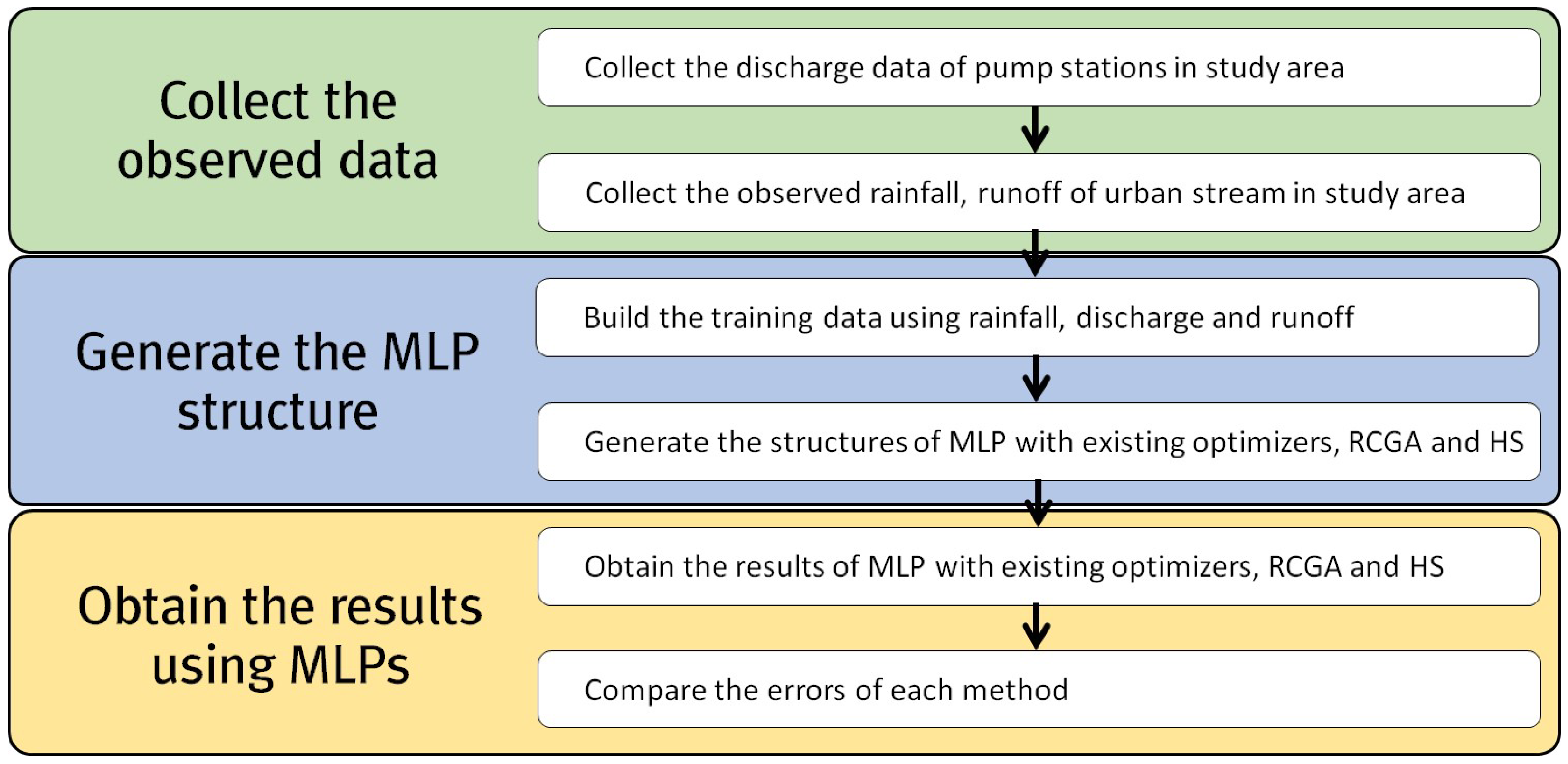
The study was divided into three steps:
- The observed rainfall data, the discharge of each pump station, and the runoff of the urban stream were collected.
- The structures of MLPHS were generated to predict the runoff of urban streams.
- The MLPHS results were compared with the results of the MLP with existing optimizers and the RCGA.
Figure 1 illustrates the steps followed in this study to predict the runoff of urban stream.
2.2. Study Area
The Han River, which penetrates Seoul (the capital of South Korea), has various tributaries such as the Anyang and Hongje streams, and the Anyang Stream has tributaries such as the Mokgam and Dorim streams. In the Dorim stream, this study focused on two tributaries (Daebang and Bongchun streams) and 11 pump stations (Mullae, Dorim2, Daerim2, Daerim3, Guro1, Guro2, Guro3, Guro4, Sinlim1, Sinlim2, and Sinlim5 pump stations). The discharged stream of the 11 pump stations is the Dorim Stream. The Daebang and Bongchun streams had no pump stations. The Dorim stream starts at Seoul National University, located on Gwanak Mountain, the upstream point, and continues to the downstream point of the Anyang Stream junction. The monitoring point for observing the runoff of the Dorim Stream is located downstream. In addition, an observatory for rainfall observations was located in the middle of the watershed. The drainage area (A), length (L), and shape coefficient (A/L2) of the Dorim stream are 41.93 km2, 14.2 km, and 0.21, respectively. The watershed slope of the Dorim Stream ranges from 0.007 to 0.8598. Figure 2 shows information about the study area.
The drainage area of the 11 pump stations in the Dorim stream is 8.84 km2, which is approximately 21% of the total drainage area of the Dorim stream. The length of the Daebang stream is 7.16 km, and the length of the Bongchun stream is 5.00 km. The Gwanak detention reservoir is located upstream of the Dorim stream and has a capacity of 65,000 m3. The drainage area of the 11 pump stations varies from 0.19 km2 to 2.49 km2. The basin of the Daerim3 pump station, which has the largest drainage area, has a Daerim detention reservoir for flood reduction. The capacity of the Daerim detention reservoir is 2447 m3. Table 1 lists the drainage areas of each pump station.
In Table 1, the Daerim3 pump station had the largest drainage area of 2.49 km2, whereas the Daerim2 pump station had the smallest drainage area of 0.19 km2. Pump stations are drained naturally through a sluice gate or drained through drainage pumps. A detention reservoir was constructed in the drainage area of the Daerim3 pump station, which has the largest drainage area.
2.3. Preparation of Data for the MLPHS
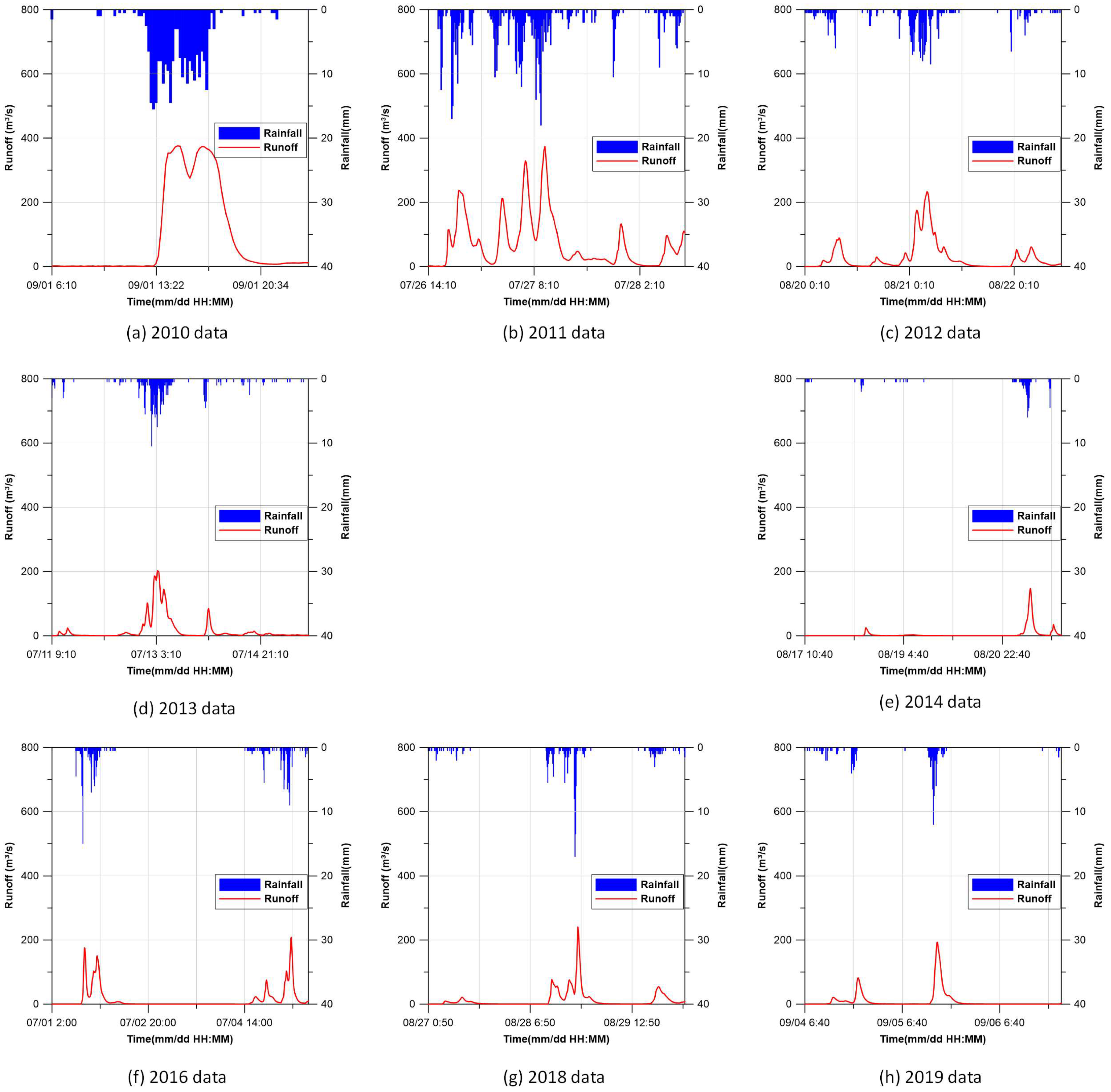
Prior to being applied to the MLPHS, data from 2010, 2011, 2012, 2013, 2014, 2016, 2018, and 2019, when rainfall occurred most recently in the study area, were prepared. The interval of the observed runoff in the Dorim stream was 10 min. During the rest of the period, it is difficult to construct appropriate learning data as the pumps at each pump station did not operate. If the data of each pump station when the pumps were not operated is used as the learning data, the learning may not work properly. Since the data for each year are different, it is difficult to guarantee accurate prediction results when the raw data is used at it is. To compensate such shortcomings using raw data, in this study, the prediction accuracy was improved by using normalization. Figure 3 shows the observed rainfall and runoff data from 2010 to 2019.
Data from 2010 to 2018 were used as the learning dataset for the MLP, and data from 2019 were used for making predictions. In addition to these data, records of rainfall received in the study area were used; however, data from pump stations that were not operated due to the low water level of the stream were excluded.
For efficient learning of the MLP, normalization was conducted to represent each data set as a value between 0 and 1. The normalization is shown in Equation (1).
where yi is the normalized value, and xi is the real value. xmax is the maximum real value, and xmin is the minimum real value. To compare the results of each MLP, the square value-based root mean square error (RMSE) and absolute value-based mean absolute error (MAE) and R-squared (R2) were applied. The RMSE, MAE, and R2 equations are given by Equation (A1), Equation (A2), and Equation (A3), respectively in Appendix A.
2.4. Multi-Layer Perceptron Combined with the Harmony Search
Machine learning techniques, including multi-layer perceptrons, are used to predict or classify data. For example, a computer cannot distinguish a dog from a cat using only a picture; however, humans can easily distinguish between dogs and cats. For this purpose, a machine learning method was developed. With machine learning, a large amount of data is inputted into a computer and then used to classify similar data. When a picture similar to a stored picture of a dog is input, the computer classifies the picture as a dog. Many machine learning algorithms have been developed to classify data. Representative examples include decision trees, Bayesian networks, SVMs, and ANNs. Among them, deep learning methods are the descendants of ANNs.
A perceptron was proposed as a type of ANN [1]. A single-layer perceptron can predict linearly separable things; however, the calculation of XOR is not possible. A multi-layer perceptron has been proposed to overcome the limitation of a single-layer perceptron. As it can predict non-linearly separable things, it can be used to calculate XOR. Linear separation is possible with a single neuron in a single-layer perceptron. In a multi-layer perceptron, the number of neurons is higher than that in a single-layer perceptron, and layers are added to create a complex decision boundary structure.
In the MLP, the optimizer is a tool applied to the gradient descent using differentiation to consider the optimization of correlations between neurons. As the use of ANNs, including multi-layer perceptrons, has become more widespread, the importance of optimizers that can efficiently find optimal correlations has increased. The optimizers commonly used in ANNs are the gradient descent (GD), stochastic gradient descent (SGD), adaptive gradient (Adagrad), root mean squared propagation (RMSprop), adaptive delta (AdaDelta), adaptive moment (Adam), and Nesterov-accelerated adaptive moment (Nadam). Existing optimizers, including the GD, SGD, Adagrad, RMSprop, AdaDelta, Adam, and Nadam depend entirely on the shape of the error surface and the weights and biases that are initially created. There is a possibility of convergence to the local optimum as new weights and biases are generated using the numerical derivative. To overcome the shortcomings of the existing optimizers, the MLP was improved by applying a meta-heuristic optimization algorithm that can consider global and local searches.
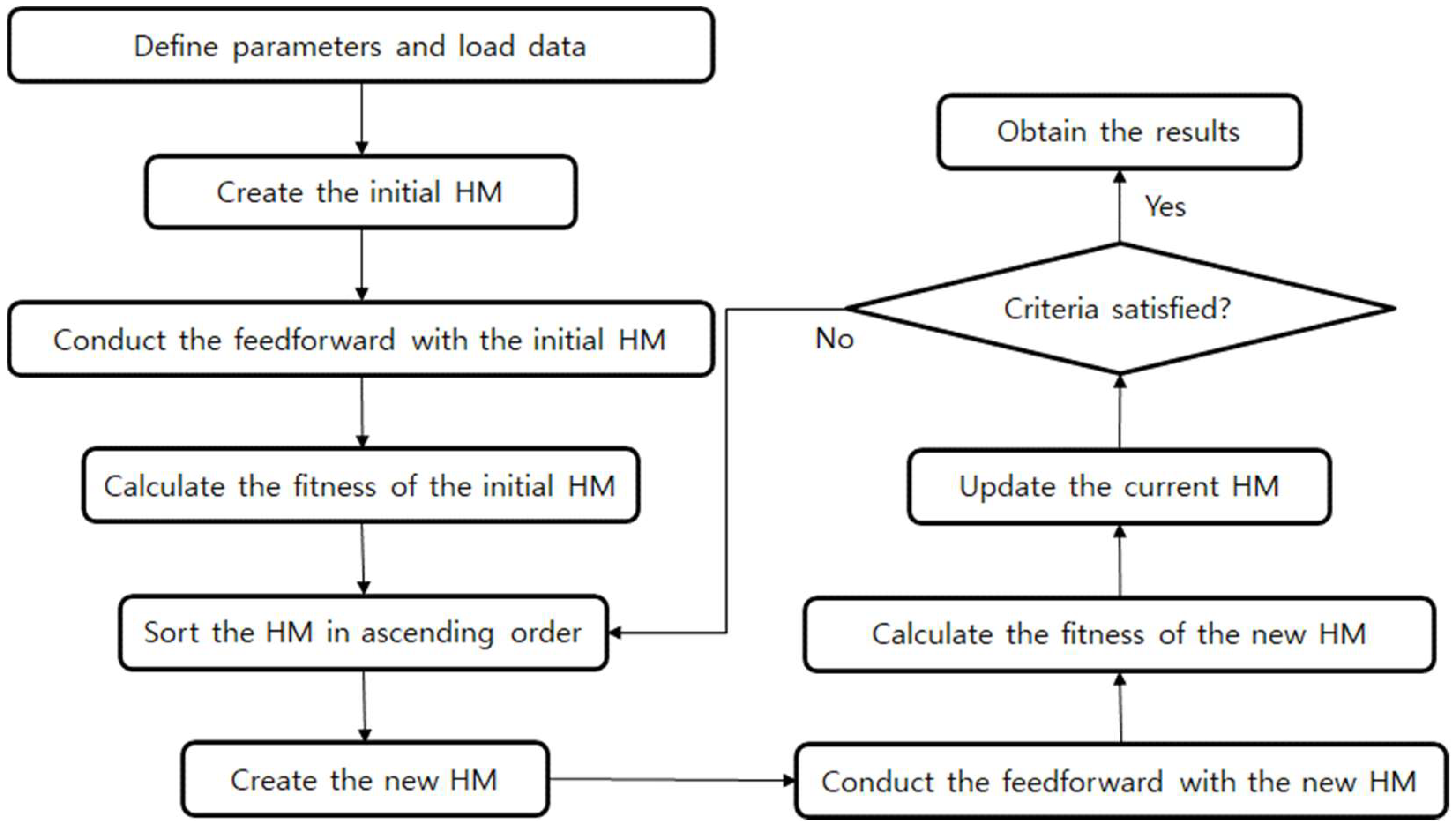
The HS is a meta-heuristic optimization algorithm motivated by the improvisation of musicians. The parameters of the HS are the harmony memory size (HMS), harmony memory considering rate (HMCR), pitch adjustment rate (PAR), and bandwidth (BW). The HMS is the size of the HM. The number of initially randomly generated solutions was determined according to the HMS. The HMCR is the probability of choosing a decision variable within the HM. The process used to create a new decision variable by randomly combining the decision variables in the current HM is similar to the operation process of the GA. However, the GA always creates a new decision variable from two decision variables. The HS, on the other hand, can create a new decision variable from two or more decision variables as well as the HMS. Additionally, the GA cannot consider decision variables independently as it should maintain the genetic structure; however, the HS can select each decision variable independently when generating a new solution. The PAR is the probability of selecting a new decision variable adjacent to the previously selected decision variable through the HMCR while considering the BW. To compare the results of MLP using the existing optimizers, MLP using the RCGA and MLPHS, the structure of MLP was set to five hidden layers, and ten nodes in each hidden layer were set. Figure 4 shows the calculation flow of the MLPHS used in this study.
3. Application and Results
Comparison of Results
Data from 2010 to 2018 were used to train the MLP model. Data from 2019 were used to predict the runoff and rainfall information. A rectified linear unit (ReLU) was used as the activation function in the MLP using existing optimizers, MLP using RCGA, and MLPHS. Each MLP learned 100,000 epochs of data from 2010 to 2018 and then predicted the results of 2019. The results obtained using each MLP were then compared. Among the parameters of the RCGA, the population was set to 50, and the mutation rate was set to 0.15. HMS, HMCR, PAR, and BW in the HS were set to 50, 0.85, 0.4, and 0.0003, respectively. In the GA and HS, the searching range of weights and biases was set from −15 to 15. Table 2 shows the results obtained with MLP using existing optimizers, MLP using the RCGA, and MLPHS.
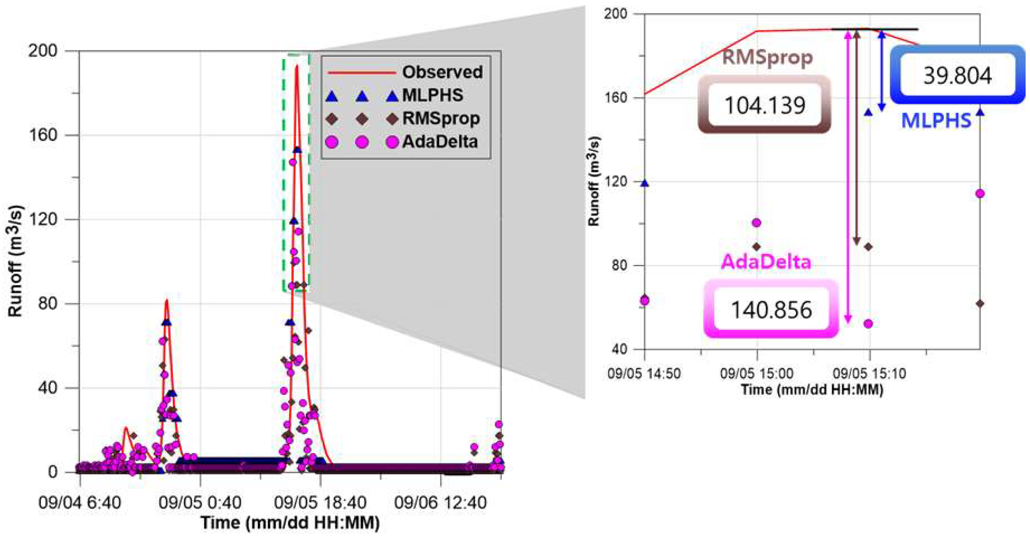
Among the existing optimizers, the AdaDelta was the best for the RMSE and RMSprop was the best for the MAE, and Nadam showed the highest R2. However, in all the results including MLP using the RCGA and MLPHS, RMSE and MAE of MLPHS were the lowest, and MLPHS showed the highest value in R2. The results of the AdaDelta and RMSprop, which gave good results among the applied optimizers, for each time period were compared with those obtained with the MLPHS. Figure 5 shows a comparison of the results obtained with the AdaDelta, RMSprop, and HS (MLPHS).
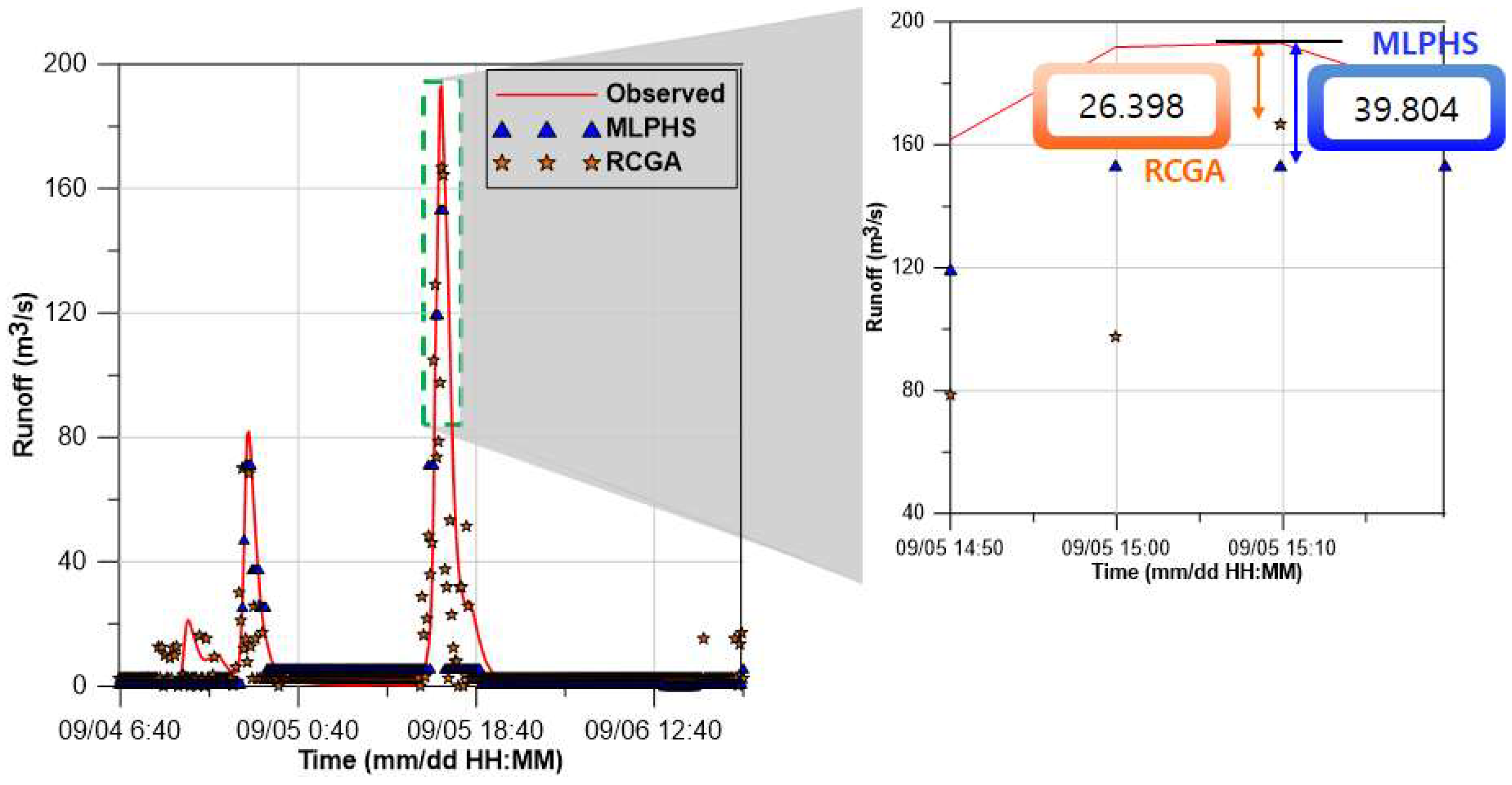
Additionally, notable results occurred at the peak value of the observed runoff. RMSprop showed a difference of 104.139 m3/s from the peak value of the observed runoff, and AdaDelta showed a difference of 140.856 m3/s from the peak value of the observed runoff. On the other hand, the MLPHS showed a difference of 39.804 m3/s from the peak value of the observed runoff. The MLPHS showed better results than the existing optimizers in terms of both overall and peak results. The results of the MLP using the RCGA were compared with those of the MLPHS. Figure 6 shows a comparison of the results obtained with the MLP using the RCGA and the HS (MLPHS).
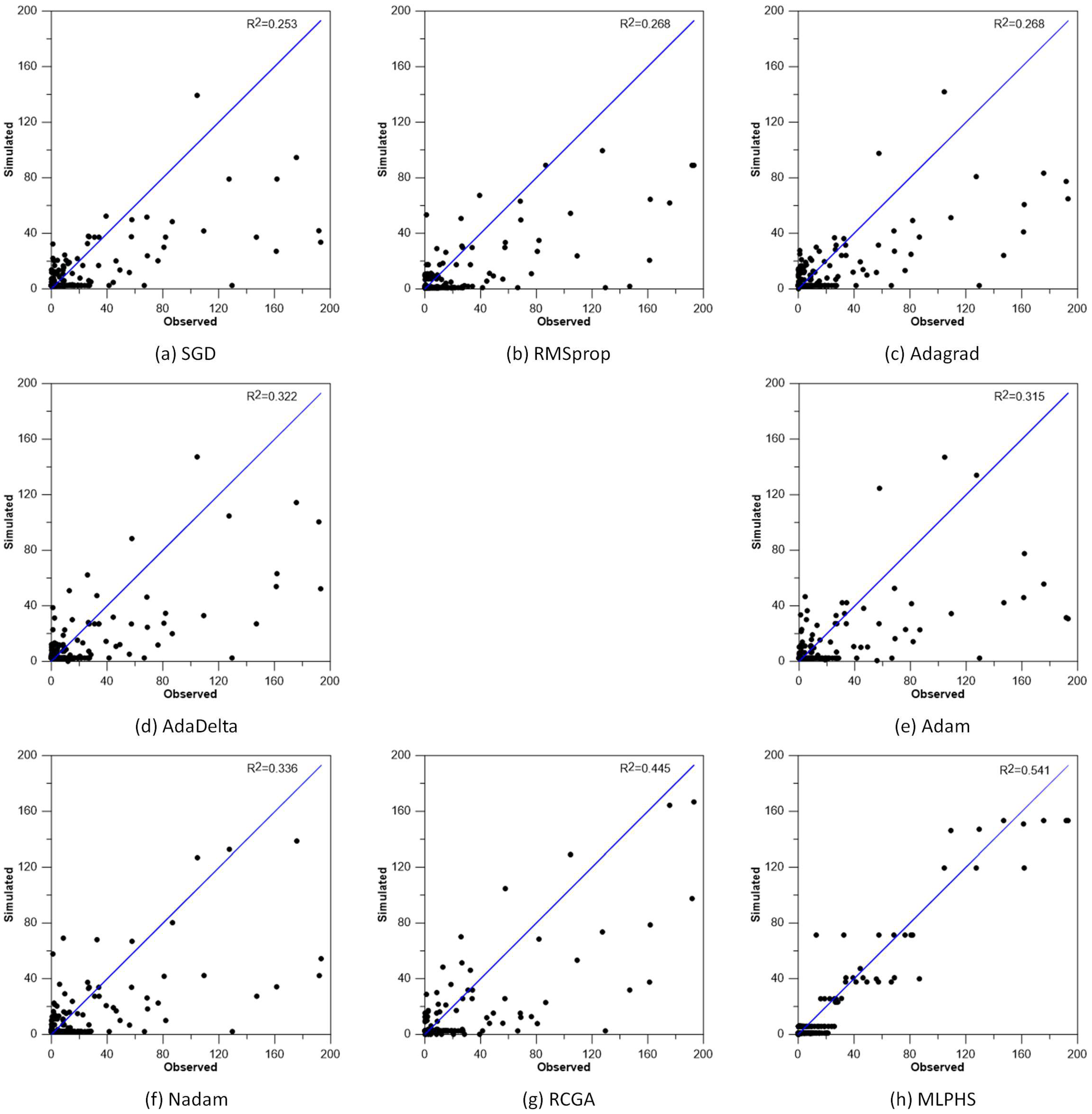
The MLP using the RCGA showed a difference of 26.398 m3/s from the peak value of the observed runoff, and the MLPHS showed a difference of 39.804 m3/s from the peak value of the observed runoff. At the peak value of the observed runoff, the MLP using the RCGA showed better results than the MLPHS. However, in the observed runoff near the peak value, the MLP using the RCGA showed a larger error than the MLPHS. Considering the overall results, the MLPHS provided the most accurate prediction among all the applied optimizers. Figure 7 shows the R2 for the observed and predicted data of MLP using the existing optimizers, MLP using RCGA, and MLPHS.
4. Discussion
In general, in most studies, the results of the new study were compared with those of previous studies. However, since there are no results obtained in previous studies, the learning time required for MLP using the existing optimizers, MLP using RCGA, and MLPHS, was compared. To compare the required time, only data from 2010 was used, and the epochs were set to 1000. In addition, the learning of each MLP was repeated 50 times to calculate the average value.
The time required according to the number of nodes was simulated by setting the hidden layer to one and the number of nodes from one to five. Additionally, the time required according to the number of hidden layers was simulated with three nodes and one to five hidden layers. Table 3 showed the average time required for each optimizer according to the number of nodes.
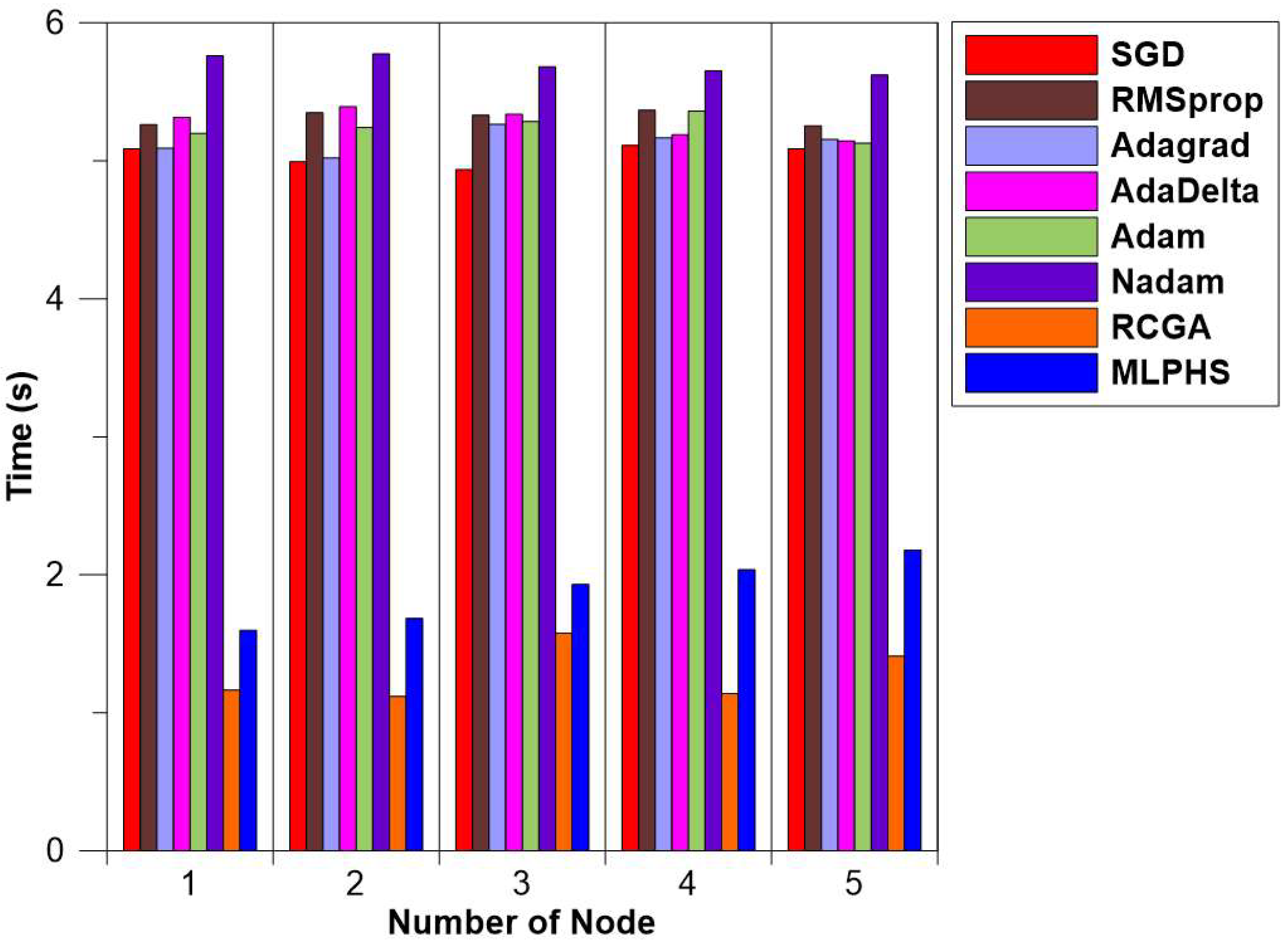
Figure 8 shows the comparison of the average time required for each optimizer according to the number of nodes.
According to the results of Table 3 and Figure 8, MLP using the RCGA showed the shortest average time required for the number of nodes from one to five, and MLPHS showed the second shortest average time. Table 4 shows the average time required for each optimizer according to the number of hidden layers.
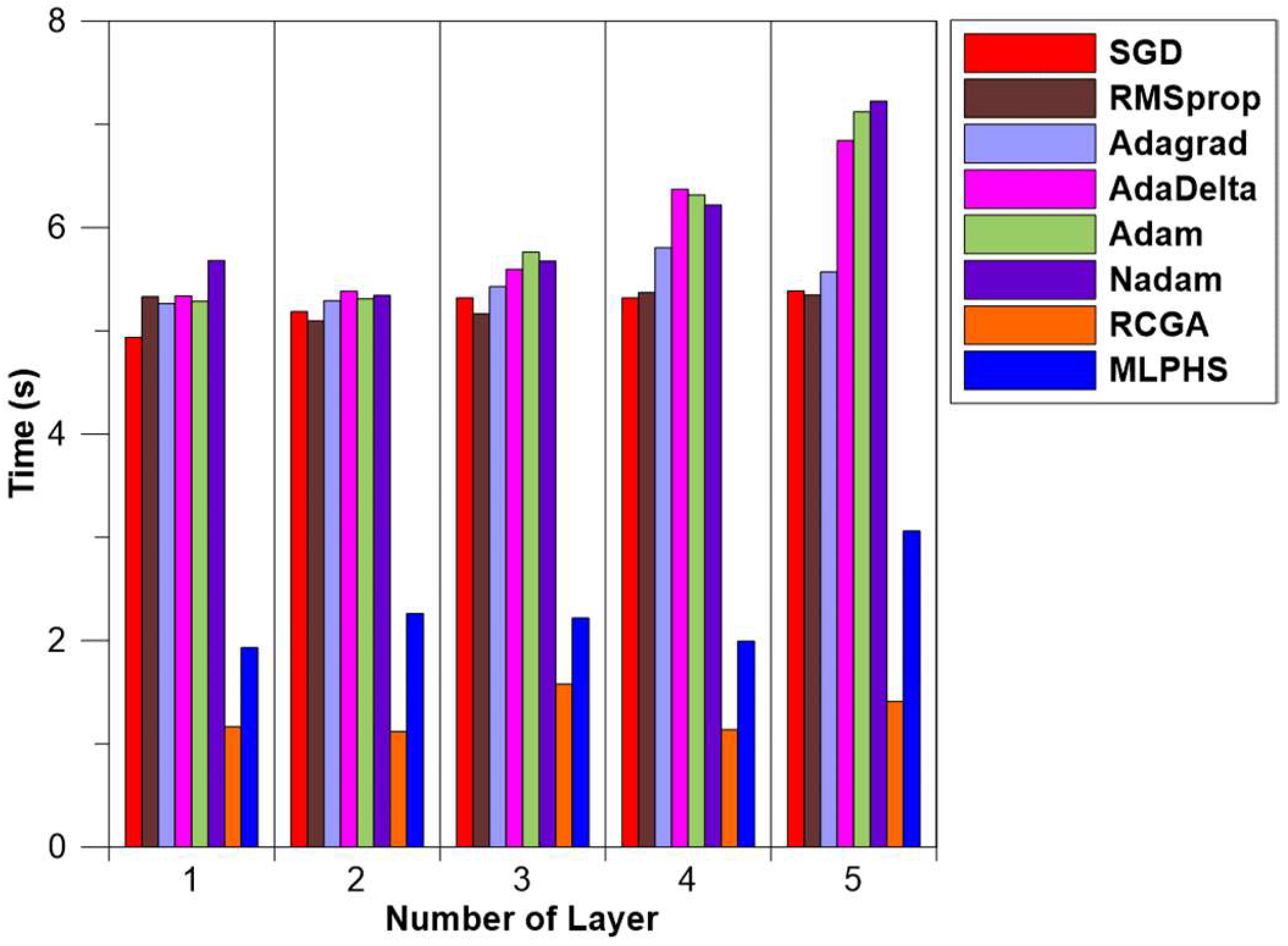
Figure 9 shows the comparison of the average time required for each optimizer according to the number of hidden layers.
According to the results of Table 4 and Figure 9, MLP using the RCGA showed the shortest average time required for the number of nodes from one to five, and MLPHS showed the second shortest average time. These results were similar to the average time required for each optimizer according to the number of nodes. The existing optimizer finds a new solution by updating the weight and bias of the existing solution position using differentiation. However, meta-heuristic optimization algorithms such as RCGA and HS find a new solution through a combination of existing solutions, fine-tuning, or random selection in the search range. The reason the amount of time required for MLP using the meta-heuristic optimization algorithm was shorter than that of MLP using the existing optimizers is due to the difference in the search method for a new solution. Additionally, the average time required was longest when the number of hidden layers was five and the number of nodes was three. Therefore, the average time required is long when the calculation process is long due to the large number of weights and biases.
5. Conclusions
The MLP using existing optimizers, MLP using RCGA, and MLPHS, were applied to predict urban stream runoff, and discharge from each pump station was used as the learning data. The data from 2010 to 2018 were used as the learning data, and the predicted results for 2019 obtained with the MLPHS were more accurate than the results obtained with the MLP using existing optimizers and MLP using RCGA. Among the results of the MLP using existing optimizers, those obtained with the MLP using AdaDelta exhibited the smallest RMSE, and those obtained with the MLP using RMSprop exhibited the smallest MAE. In addition, MLP using Nadam among MLP using the existing optimizers showed the highest R2.
The results of the study revealed that the discharge of pump stations in urban areas can be used to predict the runoff of urban streams. Pump stations have been constructed in urban areas to prevent urban flooding. The results revealed that the discharge of pump stations directly affects the amount of runoff from urban streams as pump stations discharge water from the inland to urban streams.
The results of the study revealed that the MLPHS can be applied to reduce the error between the observed and simulated runoff. The optimizer of the MLP is a very important component of the learning process. As the optimizer greatly influences the weights and biases in the MLP, studying how the optimizer can be improved is very important. In this study, learning was conducted by replacing the optimizer used in the MLP with the HS, a well-known metaheuristic optimization algorithm.
A limitation of this study is that the observation data consisted of only the runoff from each pump station and rainfall. In future studies, more accurate runoff predictions would be possible if the water level or runoff observation data at the upstream point were added. Additionally, it is possible to increase usability by applying a self-adaptive meta-heuristic optimization algorithm. Learning using the MLP can be conducted if an automatic optimization of the MLP structure can be performed.
Author Contributions
W.J.L. and E.H.L. carried out the literature survey and drafted the manuscript; E.H.L. worked on subsequent drafting the manuscript; W.J.L. performed the simulations; E.H.L. conceived the original idea of the proposed method. All authors have read and agreed to the published version of the manuscript.
Funding
This research was funded by the National Research Foundation (NRF) of Korea (NRF-2019R1I1A3A01059929).
Institutional Review Board Statement
Not applicable.
Informed Consent Statement
Not applicable.
Acknowledgments
This work was supported by the National Research Foundation (NRF) of Korea (NRF-2019R1I1A3A01059929).
Conflicts of Interest
The authors declare no conflict of interest.
Abbreviations
| MLP | Multi-layer perceptron |
| MLPHS | Multi-layer perceptron using harmony search |
| RCGA | Real coded genetic algorithm |
| ANN | Artificial neural network |
| SOM | Self-organizing map |
| CNN | Convolutional neural network |
| RNN | Recurrent neural network |
| LSTM | Long short-term memory |
| GRU | Gated recurrent unit |
| DNN | Deep neural network |
| SVM | Support vector machine |
| KNN | K-nearest neighbor |
| EA | Evolutionary algorithms |
| SA | Simulated annealing |
| ACO | Ant colony optimization |
| PSO | Particle swarm optimization |
| FA | Firefly algorithm |
| GA | Genetic algorithm |
| HS | Harmony search |
| RMSE | Root mean square error |
| MAE | Mean absolute error |
| R2 | R-squared |
| GD | Gradient descent |
| SGD | Stochastic gradient descent |
| Adagrad | Adaptive gradient |
| RMSprop | Root mean squared propagation |
| AdaDelta | Adaptive delta |
| Adam | Adaptive moment |
| Nadam | Nesterov-accelerated adaptive moment |
| HMS | Harmony memory size |
| HMCR | Harmony memory considering rate |
| PAR | Pitch adjustment rate |
| BW | Bandwidth |
| ReLU | Rectified linear unit |
Appendix A
To compare the results of each MLP, the square value-based root mean square error (RMSE) and absolute value-based mean absolute error (MAE) were applied. The RMSE equation is given by Equation (A1).
where yo is the observed value, ys is the simulated value, and n is the number of data points. The MAE equation is shown in Equation (A2).
where yo is the observed value, ys is the simulated value, and n is the number of data points. The equation of R2 is shown in Equation (A3).
where is the average of the observed value.
References
- Rosenblatt, F. The perceptron: A probabilistic model for information storage and organization in the brain. Psychol. Rev. 1958, 65, 386. [Google Scholar] [CrossRef] [Green Version]
- Kohonen, T. Self-organized formation of topologically correct feature maps. Biol. Cybern. 1982, 43, 59–69. [Google Scholar] [CrossRef]
- Hebb, D.O. The Organization of Behavior: A Neuropsychological Theory; Wiley: New York, NY, USA, 1949. [Google Scholar]
- Hopfield, J.J. Neural networks and physical systems with emergent collective computational abilities. Proc. Nat. Acad. Sci. USA 1982, 59, 2554–2558. [Google Scholar] [CrossRef] [Green Version]
- Pearl, J. Probabilistic Reasoning in Intelligent Systems: Networks of Plausible Inference; Morgan Kaufmann: San Mateo, CA, USA, 1988. [Google Scholar]
- LeCun, Y.; Bottou, L.; Bengio, Y.; Haffner, P. Gradient-based learning applied to document recognition. Proc. IEEE 1998, 86, 2278–2324. [Google Scholar] [CrossRef] [Green Version]
- Rumelhart, D.E.; Hinton, G.E.; Williams, R.J. Learning representations by back-propagating errors. Nature 1986, 323, 533–536. [Google Scholar] [CrossRef]
- Hochreiter, S.; Schmidhuber, J. Long short-term memory. Neural Comput. 1997, 9, 1735–1780. [Google Scholar] [CrossRef]
- Chung, J.; Gulcehre, C.; Cho, K.; Bengio, Y. Empirical evaluation of gated recurrent neural networks on sequence modeling. arXiv 2014, arXiv:1412.3555. [Google Scholar]
- Sit, M.; Demiray, B.Z.; Xiang, Z.; Ewing, G.J.; Sermet, Y.; Demir, I. A comprehensive review of deep learning applications in hydrology and water resources. Water Sci. Technol. 2020, 82, 2635–2670. [Google Scholar] [CrossRef]
- Worland, S.C.; Steinschneider, S.; Asquith, W.; Knight, R.; Wieczorek, M. Prediction and inference of flow duration curves using multioutput neural networks. Water Resour. Res. 2019, 55, 6850–6868. [Google Scholar] [CrossRef] [Green Version]
- Sankaranarayanan, S.; Prabhakar, M.; Satish, S.; Jain, P.; Ramprasad, A.; Krishnan, A. Flood prediction based on weather parameters using deep learning. J. Water Clim. Chang. 2020, 11, 1766–1783. [Google Scholar] [CrossRef]
- Bui, D.T.; Hoang, N.D.; Martínez-Álvarez, F.; Ngo, P.T.T.; Hoa, P.V.; Pham, T.D.; Samui, P.; Costache, R. A novel deep learning neural network approach for predicting flash flood susceptibility: A case study at a high frequency tropical storm area. Sci. Total Environ. 2020, 701, 134413. [Google Scholar]
- Bui, Q.T.; Nguyen, Q.H.; Nguyen, X.L.; Pham, V.D.; Nguyen, H.D.; Pham, V.M. Verification of novel integrations of swarm intelligence algorithms into deep learning neural network for flood susceptibility mapping. J. Hydrol. 2020, 581, 124379. [Google Scholar] [CrossRef]
- Ren, T.; Liu, X.; Niu, J.; Lei, X.; Zhang, Z. Real-time water level prediction of cascaded channels based on multilayer perception and recurrent neural network. J. Hydrol. 2020, 585, 124783. [Google Scholar] [CrossRef]
- He, X.; Luo, J.; Zuo, G.; Xie, J. Daily runoff forecasting using a hybrid model based on variational mode decomposition and deep neural networks. Water Resour. Manag. 2019, 33, 1571–1590. [Google Scholar] [CrossRef]
- Isikdogan, F.; Bovik, A.C.; Passalacqua, P. Surface water mapping by deep learning. IEEE J. Sel. Top. Appl. Earth Obs. Remote Sens. 2017, 10, 4909–4918. [Google Scholar] [CrossRef]
- Chen, Y.; Fan, R.; Yang, X.; Wang, J.; Latif, A. Extraction of urban water bodies from high-resolution remote-sensing imagery using deep learning. Water 2018, 10, 585. [Google Scholar] [CrossRef] [Green Version]
- Moy de Vitry, M.; Kramer, S.; Wegner, J.D.; Leitão, J.P. Scalable flood level trend monitoring with surveillance cameras using a deep convolutional neural network. Hydrol. Earth Syst. Sci. 2019, 23, 4621–4634. [Google Scholar] [CrossRef] [Green Version]
- Bhola, P.K.; Nair, B.B.; Leandro, J.; Rao, S.N.; Disse, M. Flood inundation forecasts using validation data generated with the assistance of computer vision. J. Hydroinform. 2019, 21, 240–256. [Google Scholar] [CrossRef] [Green Version]
- Wang, J.H.; Lin, G.F.; Chang, M.J.; Huang, I.H.; Chen, Y.R. Real-time water-level forecasting using dilated causal convolutional neural networks. Water Resour. Manag. 2019, 33, 3759–3780. [Google Scholar] [CrossRef]
- Hussain, D.; Hussain, T.; Khan, A.A.; Naqvi, S.A.A.; Jamil, A. A deep learning approach for hydrological time-series prediction: A case study of Gilgit river basin. Earth Sci. Inform. 2020, 13, 915–927. [Google Scholar] [CrossRef]
- Wang, Y.; Fang, Z.; Hong, H.; Peng, L. Flood susceptibility mapping using convolutional neural network frameworks. J. Hydrol. 2020, 582, 124482. [Google Scholar] [CrossRef]
- Van, S.P.; Le, H.M.; Thanh, D.V.; Dang, T.D.; Loc, H.H.; Anh, D.T. Deep learning convolutional neural network in rainfall-runoff modelling. J. Hydroinform. 2020, 22, 541–561. [Google Scholar] [CrossRef]
- Vandaele, R.; Dance, S.L.; Ojha, V. Deep learning for the estimation of water-levels using river cameras. Hydrol. Earth Syst. Sci. Discuss. 2021, 1–29. [Google Scholar]
- Eltner, A.; Bressan, P.O.; Akiyama, T.; Gonçalves, W.N.; Marcato Junior, J. Using deep learning for automatic water stage measurements. Water Resour. Res. 2021, 57, e2020WR027608. [Google Scholar] [CrossRef]
- Baek, S.S.; Pyo, J.; Chun, J.A. Prediction of water level and water quality using a CNN-LSTM combined deep learning approach. Water 2020, 12, 3399. [Google Scholar] [CrossRef]
- Barzegar, R.; Aalami, M.T.; Adamowski, J. Coupling a hybrid CNN-LSTM deep learning model with a Boundary corrected maximal overlap discrete wavelet transform for multiscale lake water level forecasting. J. Hydrol. 2021, 598, 126196. [Google Scholar] [CrossRef]
- Hu, C.; Wu, Q.; Li, H.; Jian, S.; Li, N.; Lou, Z. Deep learning with a long short-term memory networks approach for rainfall-runoff simulation. Water 2018, 10, 1543. [Google Scholar] [CrossRef] [Green Version]
- Kratzert, F.; Klotz, D.; Brenner, C.; Schulz, K.; Herrnegger, M. Rainfall–runoff modelling using long short-term memory (LSTM) networks. Hydrol. Earth Syst. Sci. 2018, 22, 6005–6022. [Google Scholar] [CrossRef] [Green Version]
- Jung, S.; Cho, H.; Kim, J.; Lee, G. Prediction of water level in a tidal river using a deep-learning based LSTM model. J. Korea Water Resour. Assoc. 2018, 51, 1207–1216. [Google Scholar]
- Yuan, X.; Chen, C.; Lei, X.; Yuan, Y.; Adnan, R.M. Monthly runoff forecasting based on LSTM–ALO model. Stoch. Environ. Res. Risk Assess. 2018, 32, 2199–2212. [Google Scholar] [CrossRef]
- Zhang, D.; Lin, J.; Peng, Q.; Wang, D.; Yang, T.; Sorooshian, S.; Liu, X.; Zhuang, J. Modeling and simulating of reservoir operation using the artificial neural network, support vector regression, deep learning algorithm. J. Hydrol. 2018, 565, 720–736. [Google Scholar] [CrossRef] [Green Version]
- Hu, R.; Fang, F.; Pain, C.C.; Navon, I.M. Rapid spatio-temporal flood prediction and uncertainty quantification using a deep learning method. J. Hydrol. 2019, 575, 911–920. [Google Scholar] [CrossRef]
- Yang, S.; Yang, D.; Chen, J.; Zhao, B. Real-time reservoir operation using recurrent neural networks and inflow forecast from a distributed hydrological model. J. Hydrol. 2019, 579, 124229. [Google Scholar] [CrossRef]
- Yang, T.; Sun, F.; Gentine, P.; Liu, W.; Wang, H.; Yin, J.; Du, M.; Liu, C. Evaluation and machine learning improvement of global hydrological model-based flood simulations. Environ. Res. Lett. 2019, 14, 114027. [Google Scholar] [CrossRef]
- Damavandi, H.G.; Shah, R.; Stampoulis, D.; Wei, Y.; Boscovic, D.; Sabo, J. Accurate prediction of streamflow using long short-term memory network: A case study in the Brazos River Basin in Texas. Int. J. Environ. Sci. Dev. 2019, 10, 294–300. [Google Scholar] [CrossRef] [Green Version]
- Kratzert, F.; Klotz, D.; Herrnegger, M.; Sampson, A.K.; Hochreiter, S.; Nearing, G.S. Toward improved predictions in ungauged basins: Exploiting the power of machine learning. Water Resour. Res. 2019, 55, 11344–11354. [Google Scholar] [CrossRef] [Green Version]
- Qin, J.; Liang, J.; Chen, T.; Lei, X.; Kang, A. Simulating and Predicting of Hydrological Time Series Based on TensorFlow Deep Learning. Polish J. Environ. Stud. 2019, 28, 795–802. [Google Scholar] [CrossRef]
- Kratzert, F.; Klotz, D.; Shalev, G.; Klambauer, G.; Hochreiter, S.; Nearing, G. Towards learning universal, regional, and local hydrological behaviors via machine learning applied to large-sample datasets. Hydrol. Earth Syst. Sci. 2019, 23, 5089–5110. [Google Scholar] [CrossRef] [Green Version]
- Nguyen, D.H.; Bae, D.H. Correcting mean areal precipitation forecasts to improve urban flooding predictions by using long short-term memory network. J. Hydrol. 2020, 584, 124710. [Google Scholar] [CrossRef]
- Kao, I.F.; Zhou, Y.; Chang, L.C.; Chang, F.J. Exploring a Long Short-Term Memory based Encoder-Decoder framework for multi-step-ahead flood forecasting. J. Hydrol. 2020, 583, 124631. [Google Scholar] [CrossRef]
- Xiang, Z.; Yan, J.; Demir, I. A rainfall-runoff model with LSTM-based sequence-to-sequence learning. Water Resour. Res. 2020, 56, e2019WR025326. [Google Scholar] [CrossRef]
- Zuo, G.; Luo, J.; Wang, N.; Lian, Y.; He, X. Decomposition ensemble model based on variational mode decomposition and long short-term memory for streamflow forecasting. J. Hydrol. 2020, 585, 124776. [Google Scholar] [CrossRef]
- Zhu, S.; Luo, X.; Yuan, X.; Xu, Z. An improved long short-term memory network for streamflow forecasting in the upper Yangtze River. Stoch. Environ. Res. Risk Assess. 2020, 34, 1313–1329. [Google Scholar] [CrossRef]
- Ni, L.; Wang, D.; Singh, V.P.; Wu, J.; Wang, Y.; Tao, Y.; Zhang, J. Streamflow and rainfall forecasting by two long short-term memory-based models. J. Hydrol. 2020, 583, 124296. [Google Scholar] [CrossRef]
- Bai, Y.; Bezak, N.; Sapač, K.; Klun, M.; Zhang, J. Short-term streamflow forecasting using the feature-enhanced regression model. Water Resour. Manag. 2019, 33, 4783–4797. [Google Scholar] [CrossRef]
- Tran, Q.K.; Song, S.K. Water level forecasting based on deep learning: A use case of Trinity River-Texas-The United States. J. KIISE 2017, 44, 607–612. [Google Scholar] [CrossRef]
- Kumar, D.; Singh, A.; Samui, P.; Jha, R.K. Forecasting monthly precipitation using sequential modelling. Hydrol. Sci. J. 2019, 64, 690–700. [Google Scholar] [CrossRef]
- Lee, K.; Choi, C.; Shin, D.H.; Kim, H.S. Prediction of heavy rain damage using deep learning. Water 2020, 12, 1942. [Google Scholar] [CrossRef]
- Wan, X.; Yang, Q.; Jiang, P.; Zhong, P.A. A hybrid model for real-time probabilistic flood forecasting using Elman neural network with heterogeneity of error distributions. Water Resour. Manag. 2019, 33, 4027–4050. [Google Scholar] [CrossRef]
- Kabir, S.; Patidar, S.; Pender, G. Investigating capabilities of machine learning techniques in forecasting stream flow. In Institution of Civil Engineers—Water Management; Thomas Telford Ltd.: London, UK, 2020; Volume 173, pp. 69–86. [Google Scholar]
- Wu, Z.; Zhou, Y.; Wang, H.; Jiang, Z. Depth prediction of urban flood under different rainfall return periods based on deep learning and data warehouse. Sci. Total Environ. 2020, 716, 137077. [Google Scholar] [CrossRef] [PubMed]
- Srinivasulu, S.; Jain, A. A comparative analysis of training methods for artificial neural network rainfall–runoff models. Appl. Soft Comput. 2006, 6, 295–306. [Google Scholar] [CrossRef]
- Sedki, A.; Ouazar, D.; El Mazoudi, E. Evolving neural network using real coded genetic algorithm for daily rainfall–runoff forecasting. Expert Syst. Appl. 2009, 36, 4523–4527. [Google Scholar] [CrossRef]
- Nasseri, M.; Asghari, K.; Abedini, M.J. Optimized scenario for rainfall forecasting using genetic algorithm coupled with artificial neural network. Expert Syst. Appl. 2008, 35, 1415–1421. [Google Scholar] [CrossRef]
- Yeo, Y.K.; Seo, Y.M.; Lee, S.Y.; Jee, H.K. Study on Water Stage Prediction Using Hybrid Model of Artificial Neural Network and Genetic Algorithm. J. Korea Water Resour. Assoc. 2010, 43, 721–731. [Google Scholar]
- Geem, Z.W.; Kim, J.H.; Loganathan, G.V. A new heuristic optimization algorithm: Harmony search. Simulation 2001, 76, 60–68. [Google Scholar] [CrossRef]
- Nasir, M.; Sadollah, A.; Yoon, J.H.; Geem, Z.W. Comparative Study of Harmony Search Algorithm and its Applications in China, Japan and Korea. Appl. Sci. 2020, 10, 3970. [Google Scholar] [CrossRef]
- Theodossiou, N.; Kougias, I. Harmony search algorithm, Heuristic Optimization. In Hydrology, Hydraulics and Water Resources; WIT Press: Southampton, UK, 2012. [Google Scholar]
- Menzies, T.; Kocagnuneli, E.; Turhan, B.; Minku, L.; Peters, F. Sharing Daga and Models in Software Engineering; Morgan Kaufmann: San Mateo, CA, USA, 2015. [Google Scholar]
- Dubey, M.; Kumar, V.; Kaur, M.; Dao, T.P. A systematic review on harmony search algorithm: Theory, literature, and applications. Math. Probl. Eng. 2021, 2021, 5594267. [Google Scholar] [CrossRef]
- Yang, X.S. Harmony search as a metaheuristic algorithm. In Studies in Computational Intelligence; Springer: Berlin/Heidelberg, Germany, 2009; Volume 191, pp. 1–14. [Google Scholar]
Figure 1.
Application process followed to predict the runoff of urban stream.

Figure 2.
Information about the study area (Imagery © 2022 CNES/Airbus, Landsat/Copernicus, Maxar Technologies, NSPO 2021).
Figure 2.
Information about the study area (Imagery © 2022 CNES/Airbus, Landsat/Copernicus, Maxar Technologies, NSPO 2021).

Figure 3.
Observed rainfall and runoff data in Dorim stream.

Figure 4.
Calculation flow of the MLPHS.

Figure 5.
Comparison of the results obtained with AdaDelta, RMSprop, and HS (MLPHS).

Figure 6.
Comparison of the results obtained with the MLP using RCGA and the HS (MLPHS).

Figure 7.
R2 for observed and predicted data of MLP using the existing optimizers, MLP using the RCGA, and MLPHS.
Figure 7.
R2 for observed and predicted data of MLP using the existing optimizers, MLP using the RCGA, and MLPHS.

Figure 8.
Comparison of average time required for each optimizer according to the number of nodes.

Figure 9.
Comparison of average time required for each optimizer according to the number of hidden layers.
Figure 9.
Comparison of average time required for each optimizer according to the number of hidden layers.


Table 1.
Information about drainage areas.
| Location | Dorim Stream | Dorim2 Pump Station | Daerim2 Pump Station | Daerim3 Pump Station | Guro1 Pump Station | Guro2 Pump Station |
| Drainage area (km2) | 41.93 | 1.50 | 0.19 | 2.49 | 1.36 | 0.47 |
| Location | Guro3 Pump Station | Guro4 Pump Station | Mullae Pump Station | Sinlim1 Pump Station | Sinlim2 Pump Station | Sinlim5 Pump Station |
| Drainage area (km2) | 0.45 | 0.27 | 0.82 | 0.56 | 0.46 | 0.27 |
Table 2.
Results obtained with each MLP.
| Optimizer | SGD | RMSprop | Adagrad | AdaDelta | Adam | Nadam | RCGA | HS(MLPHS) |
|---|---|---|---|---|---|---|---|---|
| RMSE (m3/s) | 20.375 | 20.152 | 19.290 | 19.072 | 21.251 | 21.245 | 17.862 | 17.061 |
| MAE (m3/s) | 7.910 | 7.208 | 7.784 | 7.817 | 8.097 | 7.797 | 7.634 | 6.404 |
| R2 | 0.253 | 0.268 | 0.268 | 0.322 | 0.315 | 0.336 | 0.445 | 0.541 |
Table 3.
Average time required for each optimizer according to the number of nodes.
| Number of Nodes | 1 | 2 | 3 | 4 | 5 |
|---|---|---|---|---|---|
| SGD | 5.087 s | 4.994 s | 4.937 s | 5.112 s | 5.088 s |
| RMSprop | 5.263 s | 5.349 s | 5.331 s | 5.367 s | 5.254 s |
| Adagrad | 5.091 s | 5.020 s | 5.264 s | 5.167 s | 5.156 s |
| AdaDelta | 5.316 s | 5.392 s | 5.338 s | 5.189 s | 5.144 s |
| Adam | 5.199 s | 5.242 s | 5.286 s | 5.361 s | 5.127 s |
| Nadam | 5.761 s | 5.775 s | 5.681 s | 5.652 s | 5.622 s |
| RCGA | 1.108 s | 1.117 s | 1.164 s | 1.088 s | 1.065 s |
| MLPHS | 1.596 s | 1.683 s | 1.929 s | 2.037 s | 2.179 s |
Table 4.
Average time required for each optimizer according to the number of hidden layers.
| Number of Hidden Layers | 1 | 2 | 3 | 4 | 5 |
|---|---|---|---|---|---|
| SGD | 4.937 s | 5.185 s | 5.319 s | 5.318 s | 5.387 s |
| RMSprop | 5.331 s | 5.096 s | 5.165 s | 5.371 s | 5.346 s |
| Adagrad | 5.264 s | 5.293 s | 5.428 s | 5.805 s | 5.571 s |
| AdaDelta | 5.338 s | 5.384 s | 5.597 s | 6.371 s | 6.841 s |
| Adam | 5.286 s | 5.311 s | 5.762 s | 6.317 s | 7.120 s |
| Nadam | 5.681 s | 5.342 s | 5.675 s | 6.219 s | 7.226 s |
| RCGA | 1.164 s | 1.119 s | 1.576 s | 1.138 s | 1.409 s |
| MLPHS | 1.929 s | 2.263 s | 2.218 s | 1.994 s | 3.062 s |
Publisher’s Note: MDPI stays neutral with regard to jurisdictional claims in published maps and institutional affiliations. |
© 2022 by the authors. Licensee MDPI, Basel, Switzerland. This article is an open access article distributed under the terms and conditions of the Creative Commons Attribution (CC BY) license (https://creativecommons.org/licenses/by/4.0/).
Share and Cite
MDPI and ACS Style
Lee, W.J.; Lee, E.H. Runoff Prediction Based on the Discharge of Pump Stations in an Urban Stream Using a Modified Multi-Layer Perceptron Combined with Meta-Heuristic Optimization. Water 2022, 14, 99. https://doi.org/10.3390/w14010099
AMA Style
Lee WJ, Lee EH. Runoff Prediction Based on the Discharge of Pump Stations in an Urban Stream Using a Modified Multi-Layer Perceptron Combined with Meta-Heuristic Optimization. Water. 2022; 14(1):99. https://doi.org/10.3390/w14010099
Chicago/Turabian StyleLee, Won Jin, and Eui Hoon Lee. 2022. "Runoff Prediction Based on the Discharge of Pump Stations in an Urban Stream Using a Modified Multi-Layer Perceptron Combined with Meta-Heuristic Optimization" Water 14, no. 1: 99. https://doi.org/10.3390/w14010099
Note that from the first issue of 2016, this journal uses article numbers instead of page numbers. See further details here.