Pressure Sensor Placement in Water Supply Network Based on Graph Neural Network Clustering Method

Abstract

Pressure sensor placement is critical to system safety and operation optimization of water supply networks (WSNs). The majority of existing studies focuses on sensitivity or burst identification ability of monitoring systems based on certain specific operating conditions of WSNs, while nodal connectivity or long-term hydraulic fluctuation is not fully considered and analyzed. A new method of pressure sensor placement is proposed in this paper based on Graph Neural Networks. The method mainly consists of two steps: monitoring partition establishment and sensor placement. (1) Structural Deep Clustering Network algorithm is used for clustering analysis with the integration of complicated topological and hydraulic characteristics, and a WSN is divided into several monitoring partitions. (2) Then, sensor placement is carried out based on burst identification analysis, a quantitative metric named “indicator tensor” is developed to calculate hydraulic characteristics in time series, and the node with the maximum average partition perception rate is selected as the sensor in each monitoring partition. The results showed that the proposed method achieved a better monitoring scheme with more balanced distribution of sensors and higher coverage rate for pipe burst detection. This paper offers a new robust framework, which can be easily applied in the decision-making process of monitoring system establishment.

1. Introduction

Water supply networks, as one of the most important urban infrastructures, need to be monitored for the perspective of safety and optimized operation [1]. Considering the complex characteristics of WSNs, the monitoring system should be robust under economic constraints [2]. The reasonable and effective arrangement of pressure monitors in WSNs has attracted significant research interest in the past few years.

Heuristic methods were widely used for monitor arrangement optimization to achieve better sensitivity for the hydraulic conditions monitoring. Meier et al. [3] introduced genetic algorithms into the arrangement of monitoring sensors, transformed the arrangement of monitors into an optimization problem, and carried out experiments in a real pipe network to verify the effectiveness of the optimization method. Then, many researchers made improvements on genetic algorithms, increasing the accuracy and efficiency for monitor placement application [4,5,6]. Xiao Zhou et al. [7] considered the sensing range of the monitoring system as the objective function and used a genetic algorithm to optimize the number and location of pressure sensors based on the sensitivity matrix. Weiping Cheng et al. [8] proposed a leak detection objective function for pipe burst detection and achieved good results using a genetic algorithm to solve the objective function. In addition, Sousa et al. [9] adopted the simulated annealing algorithm, which reduced the running time compared with the genetic algorithm and achieved good results.

Conversely, the researchers also used clustering algorithms for monitoring arrangement [10,11], based on the fact that pressure fluctuation caused by demand change or pipe burst was regional in the network [12], which could be analyzed with the pressure sensitivity matrix to arrange a limited number of pressure monitors. Li Cheng [13] proposed the formula derivation for solving the pressure sensitivity matrix directly, instead of the matrix generation with nodal demand disturbance. Then, K-means [14] clustering algorithm was introduced to analyze the sensitivity matrix row vector, measure the similarity of each node, and search for the centers of each cluster as the monitoring location.

The existing research on sensor placement is mainly carried out for the following two scenarios: the first is oriented for daily management and operation optimization based on pressure monitoring data [3,7,13]. The second scenario is used for abnormal event detection in WSNs, such as pipe burst or leakage, which can be identified by the turbulence of monitoring data [8,9]. As leakage and burst detection and management is important for water supply safety [15], sensor placement analysis oriented for the second scenario is still a hot research topic in recent years.

However, due to the complex characteristics of WSNs, there are still some unresolved problems. Most of the existing research on sensor placement is only based on the analysis of hydraulic features and their fluctuations caused by demand, pipe burst or leakage [8,16,17]. However, nodal connectivity presented by network topology is also an important factor that should be considered in the evaluation of monitoring systems. The method that pays attention to only hydraulic characteristics instead of topological characteristics of the network will lead to uneven distribution of pressure sensors [18]. Another issue is that the hydraulic conditions of WSNs always change according to system operation and customer consumption. In previous studies, the sensitivity or burst recognition ability of the monitoring system was mainly analyzed based on specific operating conditions. [7,13] These existing studies have limited methods to deal with time-varying hydraulic conditions during system operation.

With the development of Graph Neural Networks (GNN) [19,20], researchers find that graph convolution can effectively combine graph topology information and feature information of nodes for cluster analysis. In 2020, Deyu Bo et al. [21] proposed the Structural Deep Clustering Network (SDCN); this algorithm introduced graph convolution operation [22,23] into the deep clustering algorithm, which enabled the clustering algorithm to be effectively expanded on graph data for the first time.

Inspired by recent research, this paper proposes a method of pressure sensor placement in WSNs based on Graph Neural Network. First, the Structural Deep Clustering Network (SDCN) [21] algorithm was used for cluster analysis with the combination of topological structure and hydraulic characteristics under multiple operating conditions, and the WSN is divided into several monitoring partitions according to cluster analysis. Then, pipe burst was simulated using hydraulic modeling, and pressure change threshold of historical monitoring data was compared with the simulated pipe burst pressure data. The most sensitive nodes were selected as sensors in each monitoring partition based on the development and analysis of a multi-dimensional quantitative metric named indicator tensor. The proposed method is verified and applied in both experimental and real-world WDNs and compared with the classical clustering algorithm for sensor placement analysis.

2. Methodology

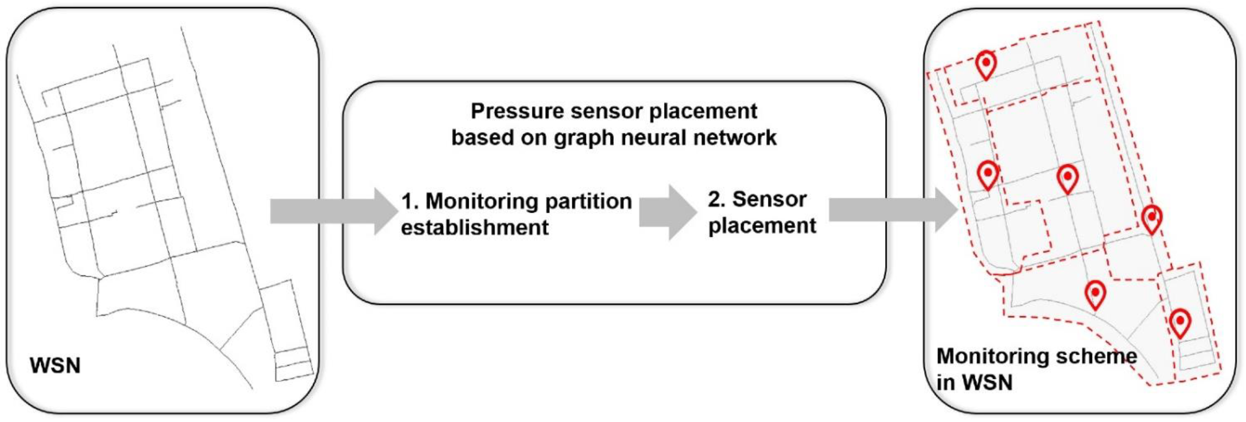
The pressure sensor placement method proposed in this paper consists of two parts, as shown in Figure 1. The first part is the establishment of monitoring partitions: SDCN algorithm is used for cluster analysis, and the WSN is divided into monitoring partitions by integrating time-dependent hydraulic characteristics and topological characteristics of the pipe network. The second part is sensor arrangement: the most sensitive nodes in each monitoring partition are selected as the sensor location according to burst identification analysis.

2.1. Monitoring Partition Establishment of WSNs

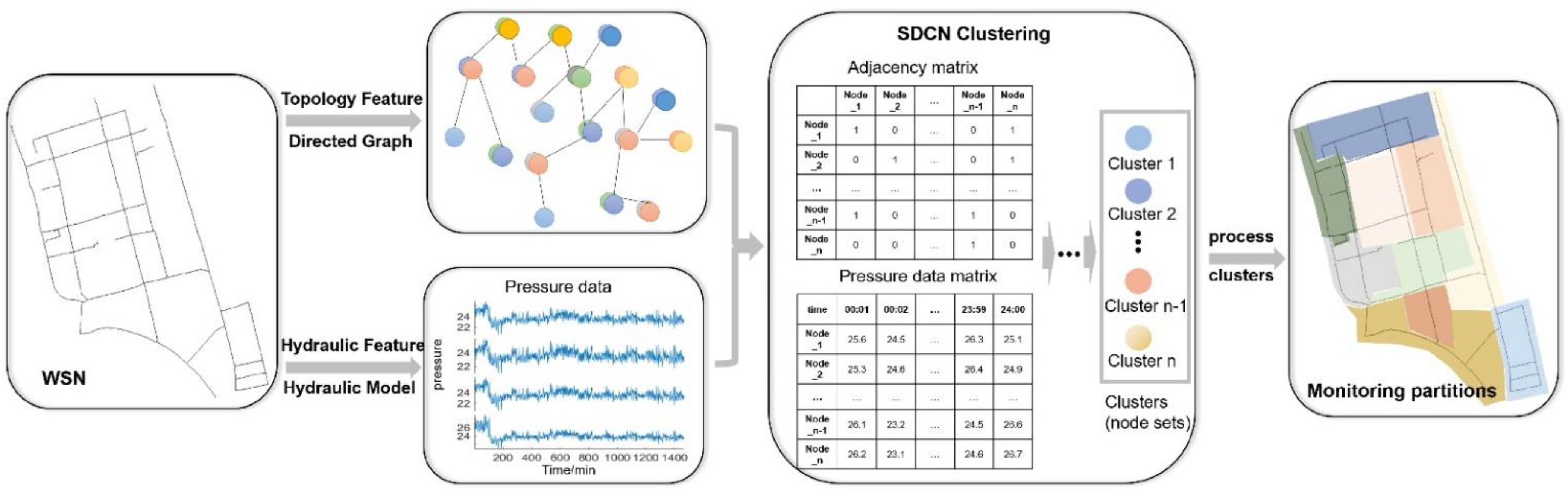
The network system can be divided into small partitions based on both nodal similarity and connectivity because of the regional characteristics in WSNs. The nodal similarity refers to the similarity of pressure and its change trends. In this paper, the clustering algorithms are used to calculate the nodal similarity through the distance between samples, which is defined by the specific algorithm [21]. In order to ensure the perception and identification ability of monitoring systems in WSN, Structural Deep Clustering Network (SDCN), a clustering algorithm based on Graph Neural Network, was used to comprehensively analyzed hydraulic and topological characteristics of WSNs.

The overall process is shown in Figure 2. The adjacency matrix and pressure data matrix of the nodes are used to represent the topological and hydraulic characteristics of the WSN respectively, and the clusters (node sets) are obtained through feature fusion with SDCN algorithm. Then, the clusters are processed according to nodal connectivity to establish spatially continuous monitoring partitions of WSN.

(1)

Hydraulic characteristics and topological characteristics

The hydraulic model of a WSN includes not only the hydraulic conditions but also the topological structure information of the WSN. The hydraulic characteristics of nodes in WSNs include pressure and demand. The pressure sensors monitor the nodal pressure directly, and change of nodal demand will cause pressure fluctuation, which can also be monitored by the pressure sensors. Therefore, in this paper, the pressure matrix P_Nodes×T (which only contains nodal pressure data) obtained with extended-period simulation is used to represent the hydraulic characteristics of WSNs, where T represents the time series length and Nodes represents the number of nodes in the WSN. A graph is the best way to represent topological structure information, and a WSN can be regarded as a directed graph with attribute values. Therefore, information such as whether the nodes are connected and the flow direction between nodes under normal operating conditions is used to construct the directed graph G of the WSN, and the adjacency matrix A_Nodes×Nodes of graph G is used to represent the topological characteristics of WSNs. The asymmetric structure of the adjacency matrix A_Nodes×Nodes contains not only the connection information of the nodes, but also the flow direction information of the pipes, which can be learned by the graph convolution operation of the SDCN [21] algorithm later.

(2)

Node clustering with SDCN algorithm

Structural Deep Clustering Network (SDCN) [21] is used in this paper to integrate hydraulic characteristics and topological characteristics of the WSNs to establish monitoring partition in WSNs. The SDCN algorithm consists of three parts: deep neural network (DNN) module, graph convolution network (GCN) module and dual self-supervised module. The DNN module adopts an auto-encoder structure to representation learning. The GCN module weighted sums the features learned by graph convolution and learned by auto-encoder, and then propagates and fuses the features on the graph structure by using multi-layer graph convolution operation. Finally, the dual self-supervised module unifies the DNN module and the GCN module in a framework, effectively performing end-to-end clustering training on them.

This article uses the SDCN algorithm implemented in the PyTorch framework (code: https://github.com/bdy9527/SDCN, accessed on 16 October 2021). SDCN algorithm is used to learn the hydraulic characteristics P_Nodes×T and topological characteristics A_Nodes×Nodes of the network. The clustering result includes clusters $C=\left[C_1,C_2,\cdots ,C_n\right]$ (also discribed as n node sets with specific features in WSNs) as well as the probability matrix Pro_Nodes×n, representing the probability that each node belongs to each cluster.

(3)

Monitoring partitions

Although SDCN algorithm takes consideration of topological connectivity of nodes in the WSN while calculating clusters, it will contain non-connected nodes in the results. To achieve spatially connected node sets in WSN, this paper adopts the following strategies to optimize clusters results, so as to obtain the final node sets $C^{\prime }=\left[C_1^{\prime },C_2^{\prime },\cdots ,C_n^{\prime }\right]$:

a. For the graph structure G_i represented by each cluster $C_i$, the node set corresponding to the largest connected subgraph in G_i is selected as the partition i and is represented as $C_i^{\prime }$, while the remaining nodes in $C_i$ are regarded as discrete points.

b. The discrete points are assigned to the nearest connected and most likely regional cluster $C_k^{\prime }$, where connectivity is judged by graph structure, and probability is judged by matrix Pro_Nodes×n.

Then, the node sets indicated by $C^{\prime }=\left[C_1^{\prime },C_2^{\prime },\cdots ,C_n^{\prime }\right]$ are used as the final monitoring partitions. The whole establishment process of monitoring partitions is shown in Algorithm 1.

Algorithm1 Monitoring partition establishment

Input: WDN’s graph G, SDCN’s clusters $C=\left[C_1,C_2,\cdots ,C_n\right]$, ProNodes×n Output: optimized clusters $C^{\prime }=\left[C_1^{\prime },C_2^{\prime },\cdots ,C_n^{\prime }\right]$ 1: S = {} 2: for $i\in \left\{1,2,\cdots ,n\right\}$ do 3:   $C_i^{\prime }=\left\{nodes | nodes=largest connected subgraph of C_i\right\}$ 4:   S append $\left\{node | node ϵ (C_i-C_i^{\prime })\right\}$ 5: end 6: repeat 7:   for $node \in S$ do 8:     for $j\in \left\{indexs=arg sort of Pr{o}_{node}\right\}$ do 9:       if {$C_j^{\prime }$, node} is connected graph do 10:         $C_j^{\prime }$ append node 11:         break 12:       end 13:     end 14:   end 15: until S is empty 16: return $C^{\prime }=\left[C_1^{\prime },C_2^{\prime },\cdots ,C_n^{\prime }\right]$

2.2. Pressure Sensor Arrangement

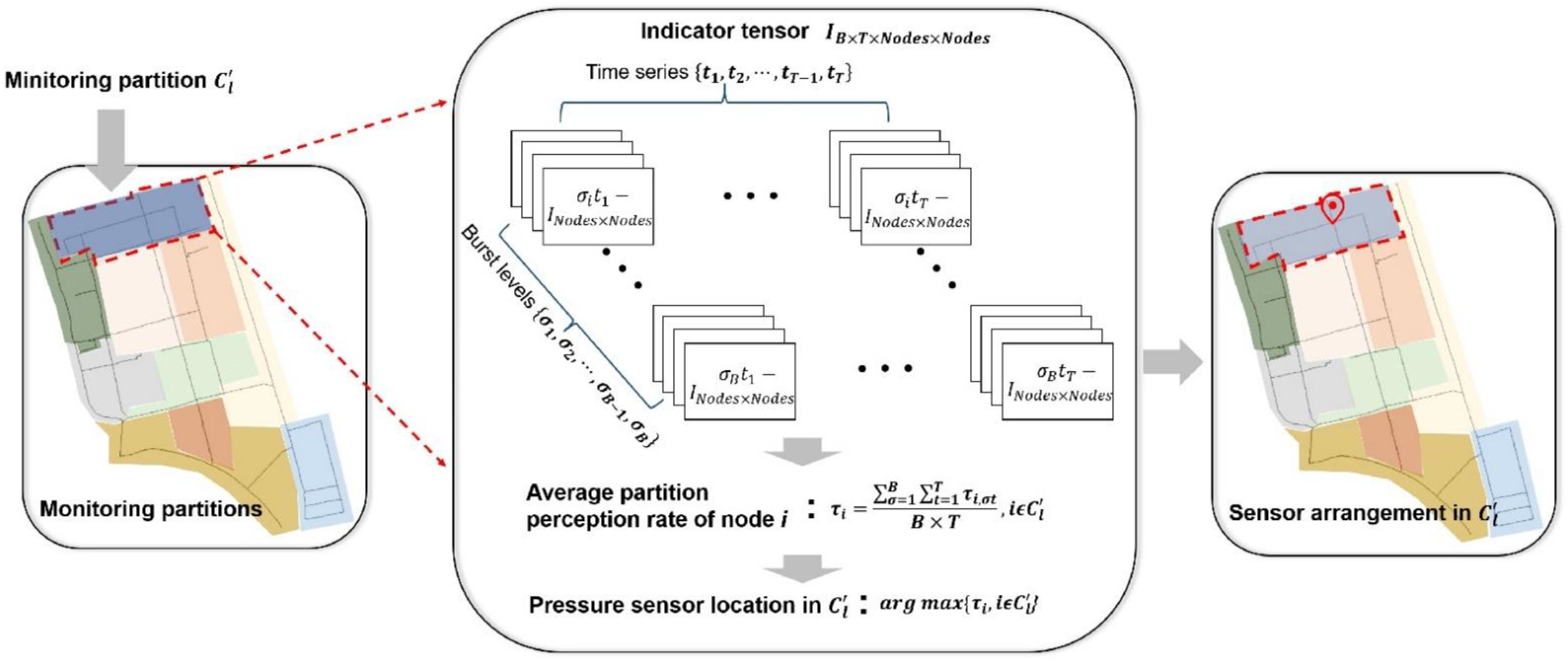
Based on the monitoring partition of the WSN, this paper assigns pressure sensors in each partition to make the arrangement of sensors more targeted for pipe burst identification. The process is shown in Figure 3. In each partition, the most sensitive node is selected as the pressure sensor according to a quantitative metric named indicator tensor generated by pipe burst identification analysis.

(1)

Pipe bursting simulation

In this paper, EPANET2.2 pressure-driven model (PDA) [24,25] is used for hydraulic simulation. By assigning the emitter coefficient c of the node, the pipe burst under different conditions is simulated.

The demand of the nodes under the PDA model is calculated by the following formula:

$$D_i^{*}=\{\begin{array}{c}0,p_i<p_i^{min}\\ D_i{\left(\frac{p_i-p_i^{min}}{p_i^{req}-p_i^{min}}\right)}^{\gamma },\\ D_i,p_i>p_i^{req}\end{array}{p}_i^{min}<p_i<p_i^{req}$$

(1)

where $D_i^{*}$ represents the actual water output of node i, $D_i$ is the water demand of node i, $p_i$ is the pressure of node i, $p_i^{min}$ and $p_i^{req}$ are the minimum pressure and demand pressure of node i, $\gamma$ is the coefficient and generally is 0.5 [26]. The $p_i^{min}$ and $p_i^{req}$ are determined according to the pressure demand of the WSN and the recommended value of the literature. In this paper, $p_i^{min}$ and $p_i^{req}$ take the values 0 and 18 m, respectively [7,26].

The pipe burst event is simulated by means of an emitter, and the calculation formula of pipe burst flow rate is as follows [27]:

$$Q_{burst}=\beta \mu \sigma A_D\sqrt{2gH}$$

(2)

where $Q_{burst}$ is the flow rate of pipe burst, the coefficient $\beta$ takes the value 0.67, the flow coefficient $\mu$ takes the value 0.61, $\sigma$ is the burst area ratio, $A_D$ is the cross-sectional area of the pipe connected to the burst node, and $H$ is the node pressure.

In the EPANET2.2 model, the emitter tool can be used to simulate the burst outflow of the node. The flow rate is described as a function of the node pressure. The formula is as follows:

$$Q_{burst}{=cH}^{\gamma }$$

(3)

where c is the emitter coefficient; γ is the pressure index.

According to Equations (2) and (3) together, the pressure index γ = 0.5, the emitter coefficient $c=\beta \mu \sigma A_D\sqrt{2g}$ and $Q_{burst}$ can be calculated with leakage area ratio and node pressure accordingly.

(2)

Indicator tensor

The occurrence of pipe burst and leakage events will reduce the pressure of some nodes and present certain regional characteristics in WSNs. Indicator tensor, a quantitative metric which describes the identification ability of each node in WSN on different operating conditions, is proposed in this paper based on the definition of pressure threshold, perception node, and indicator matrix.

(a) 

Pressure threshold:

The historical monitoring data of WSNs are analyzed, and probability density fitting on the pressure data P_k,t of node k is performed at the same time t on different days. The pressure value *P_k,t is considered the pressure threshold of node k at time t if p(P_k,t > *P_k,t) = 95%.

(b) 

Perception node:

The perception node is described as the node with a significant pressure drop when a pipe burst event occurs. The mathematical definition is as follows: When a pipe bursting event or leakage event occurs at time t, if the pressure value P_i,t of node i at time t is lower than the pressure threshold *P_i,t, then node i can identify abnormal signals and is regarded as the perception node.

(c) 

Indicator matrix:

At time t, pipe bursts at each node are simulated according to the set value of $\sigma$. With each node traversed for burst simulation, the pressure values of all nodes at time t are obtained, and the pipe burst pressure matrix σt − BP_{Nodes × Nodes} is obtained, where Nodes represents the number of nodes in a WSN hydraulic model. The σt − BP_j,i represents the pressure at point i when the burst event occurs at node j, when the time is t and the leakage area ratio is σ.

Based on the calculation of pressure matrix σt − BP_{Nodes × Nodes} and pressure threshold, the indicator matrix σt − I_{Nodes × Nodes} is defined as follows:

$$\sigma t-I_{j,i}=\{\begin{array}{c}\begin{array}{cc}1& ,\sigma t-B{P}_{j,i}<{}_{}{}^{*}P{}_{i,t}\end{array}\\ \begin{array}{cc}0& ,\sigma t-B{P}_{j,i}\ge {}_{}{}^{*}P{}_{i,t}\end{array}\end{array}i,j=1,2,\cdots ,Nodes$$

(4)

The matrix σt − I_{Nodes × Nodes} is a matrix containing only digits 0 and 1, σt − I_j,i = 1 if and only if node i is a perception node, when the time is t and the leakage area ratio is σ. The indicator matrix represents the information of the perception nodes in the WSN when the pipe burst event occurs.

(d) 

Indicator tensor:

The pipe burst event is simulated at multiple times $t\in \left\{t_1,t_2,\cdots ,t_T\right\}$ and multiple levels $\sigma \in \left\{{\sigma }_1,{\sigma }_2,\cdots ,{\sigma }_B\right\}$, and then the indicator matrix set I is obtained under the multi-hydraulic conditions. The indicator matrix set $I=\left\{{\sigma }_i{t}_j-I_{Nodes\times Nodes},i=1,\cdots ,B;j=1,\cdots ,T\right\}$ is integrated into a multi-dimensional array $I_{B\times T\times Nodes\times Nodes}$, and $I_{B\times T\times Nodes\times Nodes}$ is defined as indicator tensor I.

(3)

Pressure sensor arrangement

In order to ensure the best identification ability of sensors under different hydraulic conditions in WSNs, sensor’s arrangement is conducted according to the following steps on the basis of the indicator tensor analysis:

(1) Define nodal partition perception domain and partition perception rate. The partition perception domain of node i is a set of nodes in partition, which means that when any node in the set bursts, it will cause node i to produce a significant pressure drop. The partition perception rate of node I represents the proportion of node i’s perception domain in the entire partition. The mathematical definitions are as follows: at time t and burst level σ, given the monitoring partition $C_l^{\prime }$, for node i belonging to $C_l^{\prime }$, the node set $D_{i,\sigma t}=\left\{j\right|\sigma t-I_{j,i}=1,j\in C_l^{\prime }\}$ is called partition perception domain of the node i. The ${\tau }_{i,\sigma t}=\frac{\left|D_{i,\sigma t}\right|}{\left|C_l^{\prime }\right|}$ is called partition perception rate of node i, where $\left|D_{i,\sigma t}\right|$ and $\left|C_l^{\prime }\right|$ represent the size (number of nodes) of the node set $D_{i,\sigma t}$ and $C_l^{\prime }$.

(2) Select pressure sensor location. In monitoring partition $C_l^{\prime }$, calculate the partition perception rate ${\mathit{\tau }}_{\mathit{i},\mathit{\sigma }\mathit{t}},k ϵ C_l^{\prime }$ of node i, traverse B × T operating conditions based on indicator tensor I, and obtain the average partition perception rate of node I in the multi-hydraulic state:

$${\tau }_i=\frac{{{\displaystyle \sum }}_{\sigma =1}^B{{\displaystyle \sum }}_{t=1}^T{\mathit{\tau }}_{\mathit{i},\mathit{\sigma }\mathit{t}}}{B\times T},iϵC_l^{\prime }$$

(5)

Finally, select the node with the highest average partition perception rate in each partition $C_l^{\prime }$ as the pressure sensor in this partition.

3. Case Studies

3.1. Case 1

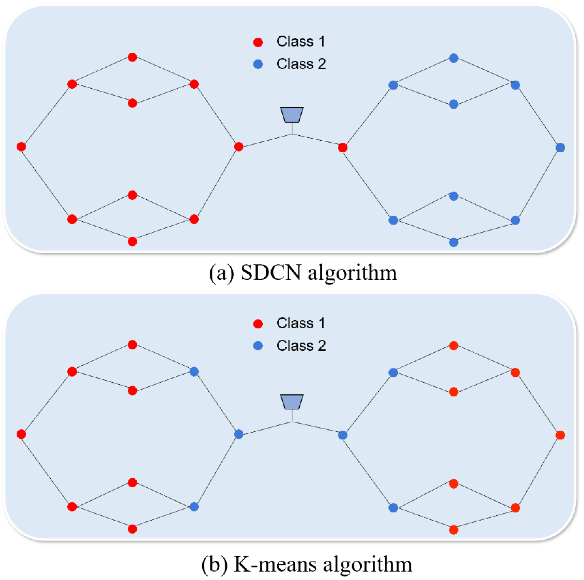
In order to verify the effectiveness and necessity of SDCN algorithm for integration of hydraulic and topological characteristics in WSN, an experimental WSN model was designed in this paper. The total simulation duration was 24 h, and the time step length was 1 h, as shown in Figure 4. The network consists of two parts in a symmetrical topology structure, connected by a reservoir in the middle. The WSN model consists of 20 nodes and 26 pipes each of which was 100 m in length. The base demand, pattern and other details of each node and pipe are shown in the Figure 4. In general, the topological characteristics are symmetric, while the hydraulic characteristics are asymmetric in this experimental WSN model.

After model simulation of 24 h duration, pressure data of each node were obtained as hydraulic characteristics P_{20 × 24}, and the adjacency matrix A_{20 × 20} of the network directed graph was used as topological characteristics. SDCN algorithm was adopted to cluster all nodes into two classes. SDCN clustering result is shown in Figure 5a. All nodes were divided into two classes, and the result is highly related to the layout of the WSN, indicating that SDCN algorithm can effectively integrate the topological and hydraulic characteristics of the WSN.

In this paper, K-means clustering algorithm was adopted for the comparison with SDCN algorithm. Only hydraulic characteristic P_{20 × 24} was used to drive K-means algorithm for clustering all nodes into two classes. The result is shown in Figure 5b. It can be clearly seen that the clustering result was highly related to the nodal pressure layout. The nodes with a short distance from the reservoir are classified into one class, with the nodes at the end of the left and right parts of the network into another. K-means algorithm extracted the hydraulic characteristics of WSNs successfully, but topological characteristics are neglected because of the algorithm limitations. Therefore, the clustering results of K-means algorithm cannot be directly used for regional monitoring and inspection of the WSN.

The clustering results of the experimental water supply network model show that SDCN algorithm can integrate topological and hydraulic characteristics of the WSN effectively, which is applicable for regional management of water supply network with complex topology structure and provides a new scenario for the application of Graph Neural Network in WSNs model analysis.

3.2. Case 2

A real-world network was employed to illustrate the application of pressure sensor placement method proposed in this paper. The case study is a sub-section network of an industrial district in eastern China with 8.2 km² service area and 16,000 m³ average daily water supply.

The network model shown in Figure 6 consists of 464 nodes and 482 pipes, with a total length of about 25.8 km. According to the monitoring data of the SCADA monitoring system, a hydraulic model with a total duration of 60 days for different hydraulic states was established and verified, including changes in hydraulic states caused by seasonal changes and pipeline network scheduling changes.

(1)

Proposed method

According to the method proposed in Section 2.1, the hydraulic model with a 60-day duration and 1-min timestep was used to obtain the hydraulic characteristics of WSN, represented by a pressure data matrix P_{86400 × 464} (with 464 nodes and 60 d × 24 h × 60 min = 86,400 records for each node).

According to the topological structure and flow direction of the WSN, the directed graph of the WSN is constructed, and the topological characteristics are obtained, which is represented by the adjacency matrix A_{464 × 464}. Considering the sparsity of the WSN topological characteristics, the number of neurons in the DNN module in the SDCN algorithm should be set larger such that the SDCN model can effectively learn the topology characteristics of the WSN. The DNN module of the SDCN algorithm is an autoencoder composed of seven linear layers, and a number of autoencoder neurons is set to 512, 256, 256, 128, 256, 256, 128 through continuous manual tuning. The other hyper-parameters are set as follows: learning rate set to 0.001, parameters optimization method set to Adam, epoch set to 360.

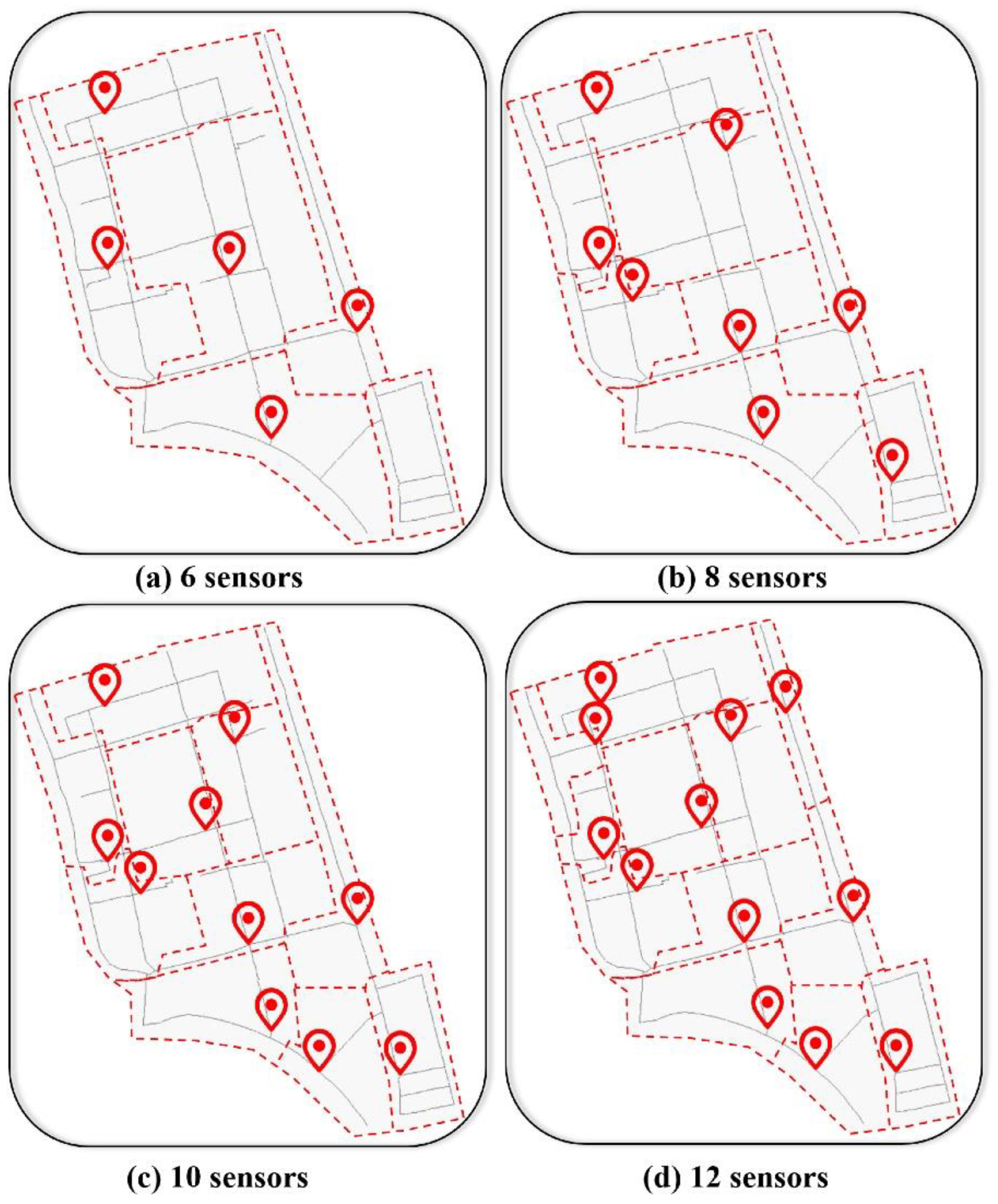
In order to analyze the identification ability of the monitoring systems with different number of sensors, the case study network is divided into 6, 8, 10 and 12 partitions, while economic constraint and conventional monitor density in WSNs is also taken into consideration. The number of cluster is set to 6, 8, 10 and 12, according to the numbers of monitoring partitions. After SDCN cluster, monitoring partitions are obtained according to the process in Algorithm 1, and the partition division results are shown in Figure 7.

In water supply networks, historical monitoring data and hydraulic models are analyzed, and the pressure threshold for each node is calculated according to the method in Section 2.2. Occurrence of pipe burst is considered to be a random event, and the pipe burst flow rate varies. In order to ensure the robustness of the monitoring system against the randomness of pipe burst event, the pipe burst simulation parameters are uniformly selected in a wide range, while calculation cost should be also taken into consideration. The pipe burst level σ is set to 0.25, 0.5, 0.75, 1.0, and time t is set to 2, 4, 6, 8, 10, 12, 14, 16, 18, 20, 22, 24 in a day, respectively. The indicator tensor I is calculated based on the burst data and the pressure threshold.

In each monitor partition, the node with the highest average partition perception rate is selected as the pressure sensor according to the method in Section 2.2. The results was shown in Figure 7.

(2)

K-means Clustering method

At present, in the research on pressure sensor placement of water supply network, the cluster method is mostly used to analyze the sensitivity matrix and determine the position of the pressure sensors at the cluster’s center. Therefore, this paper applies the method published by Li Cheng et al. [13] to compare results extracted using the proposed approach.

This method consists of two parts. The first part introduces the formula for calculating and deriving the sensitivity matrix, and the sensitivity matrix can be calculated via the formula quickly, avoiding multiple hydraulic calculations. In the second part, K-means algorithm is used to cluster the row vectors of the sensitivity matrix, and the cluster center of each category is selected as the final pressure sensor location.

In previous studies, because of the hydraulic and computational complexity of the water supply network, it was difficult to formulate simple, unified and effective evaluation indicators for the performance of the WSN monitoring system. In view of this, this paper proposes the definition and calculation formula of coverage rate to evaluate the performance of pressure sensors.

Coverage rate: The coverage rate indicates the ratio of the number of nodes that can be detected by the monitoring system to the number of nodes in the entire WSN, it can evaluate the monitoring performance of the monitoring system. The mathematical definition is as follows: at time t, the coverage rate of pressure sensors is defined as the ratio of |D| and |WDN|. |D| represents the number of elements in $D=D_{m_1,t}{\displaystyle \bigcup }{D}_{m_2,t}{\displaystyle \cup }\cdots {\displaystyle \cup }{D}_{m_m,t}$, and $D_{m_m,t}$ represents perception domain of pressure sensor $m_m$. The symbol m means the number of pressure sensors, |WDN| is the total number of nodes in the network model. The mathematical expression of coverage rate $\rho$ is as follows.

$$\rho =\frac{\left|D_{m_1,t}{\displaystyle \bigcup }{D}_{m_2,t}{\displaystyle \cup }\cdots {\displaystyle \cup }{D}_{m_m,t}\right|}{\left|WDN\right|}$$

(6)

(3)

Comparison and analysis of results

In order to verify the effectiveness of the proposed method in this paper, comparison was carried out with K-means clustering algorithm mentioned used in literature records. The sensitivity matrix of the network nodes was calculated, and the network of case study 2 was divided into 6, 8, 10, 12 clusters, with the center of each cluster chosen to be the pressure sensor location.

The monitoring placement results are shown in Figure 8, which can be compared with the monitoring arrangement obtained with SDCN method, as shown in Figure 7.

Using the K-means clustering approach to analyze the sensitivity matrix, the nodes that belong to pipes with a larger diameter in the network are more likely to be selected as pressure sensor locations, leading to more imperceptible nodes on branch pipe sections. In contrast, the sensors arranged with SDCN method are more evenly distributed in the network, which will lead to effective monitoring of branch pipe section.

In order to compare the effects of the two methods, the level of pipe bursting σ = 0.2, 0.3, 0.4, 0.5, 0.6, and the time of pipe burst t = 14:00 p.m., 12:00 p.m., 1:00 a.m. (corresponding to average flow, maximum flow and minimum flow, respectively) are set to obtain the indicator tensor under 5 × 3 = 15 different operating conditions.

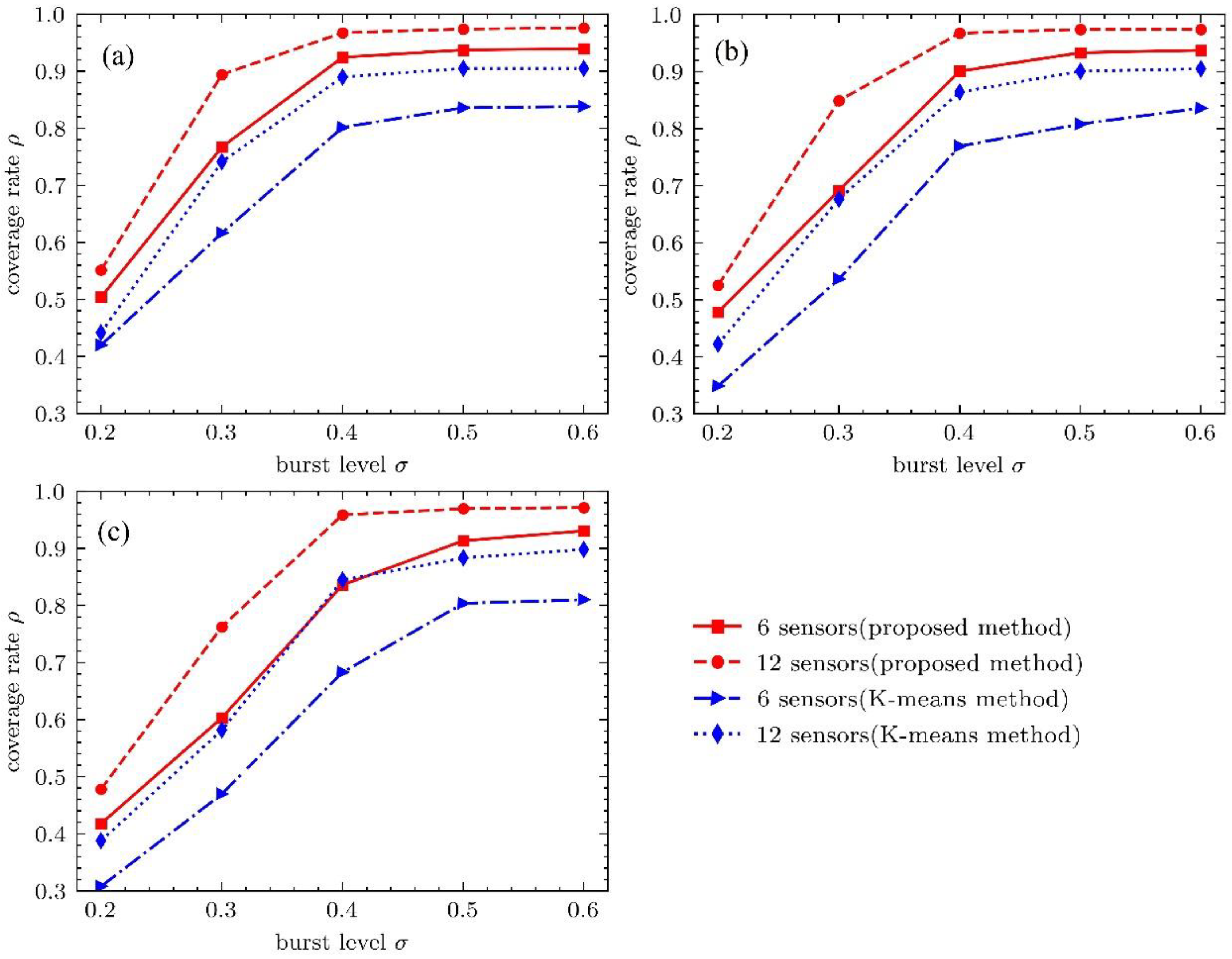
The coverage rates of sensor placement schemes with 6 and 12 monitors obtained with different methods are calculated, as shown in Figure 9. Using the same number of pressure sensors, the coverage rate of the proposed method is on average about 11% higher, which verifies the effectiveness of the proposed method.

According to Figure 9, the coverage rate of the monitoring system varies depending on hydraulic conditions. With the proposed method, the coverage rate at average flow is higher than that at maximum flow and minimum flow when the pipe burst level is lower than 0.4. This is because the sensor location selection using the proposed method is based on the calculation of the average partition perception rate and indicator tensor generated from hydraulic conditions of the WSN with 60-day duration, in which the average flow hydraulic condition has the highest probability of occurrence. With the K-means method, average flow hydraulic condition is used to calculate the sensitivity matrix and arrange monitoring sensors; thus, the coverage rate at average flow is also higher compared with other hydraulic conditions.

It can also be found that the change of hydraulic conditions has different influence on the identification ability of the monitoring system. The proposed method is robust to the change of hydraulic conditions compared with K-means method because the former takes multiple hydraulic conditions into consideration, while the latter is based on a single hydraulic time step. For example, for the monitoring scheme with six sensors at 0.2 burst level, when the hydraulic condition is switched from average flow to maximum flow, the coverage rate of the proposed method is relatively reduced by 5.1%, while the coverage rate of K-means method is relatively reduced by 16.9%. When the hydraulic condition is switched from average flow to minimum flow, the coverage rate of the proposed method and K-means method is relatively reduced by 17.1% and 26.7%, respectively. This verifies the necessity of analyzing multiple hydraulic states of the WSN and selecting the node with the highest average partition perception rate as the sensor in the partition. This phenomenon remains the same when the number of sensors is 8 and 10 and the detailed coverage rate data can be found in the Supplementary Material Tables S1 and S2.

Conversely, when the pipe burst level reaches 0.4 and higher, for three different hydraulic conditions, the nodal pressure drop caused by the pipe burst is relatively large. For each monitoring scheme, the detected nodes are generally fixed (except for the nodes far away from the sensors or on the branch pipes with small diameters which remain undetected when pipe burst reaches a certain high level); thus, the coverage rate under the three hydraulic conditions tends to be the same.

(4)

Discussion

This paper proposes a pressure sensor arrangement method based on SDCN algorithm and uses indicator tensor I and coverage rate to evaluate the performance of the monitoring system. This section discusses the influence on the coverage rate of the monitoring system with different numbers of sensors and different levels of pipe bursts.

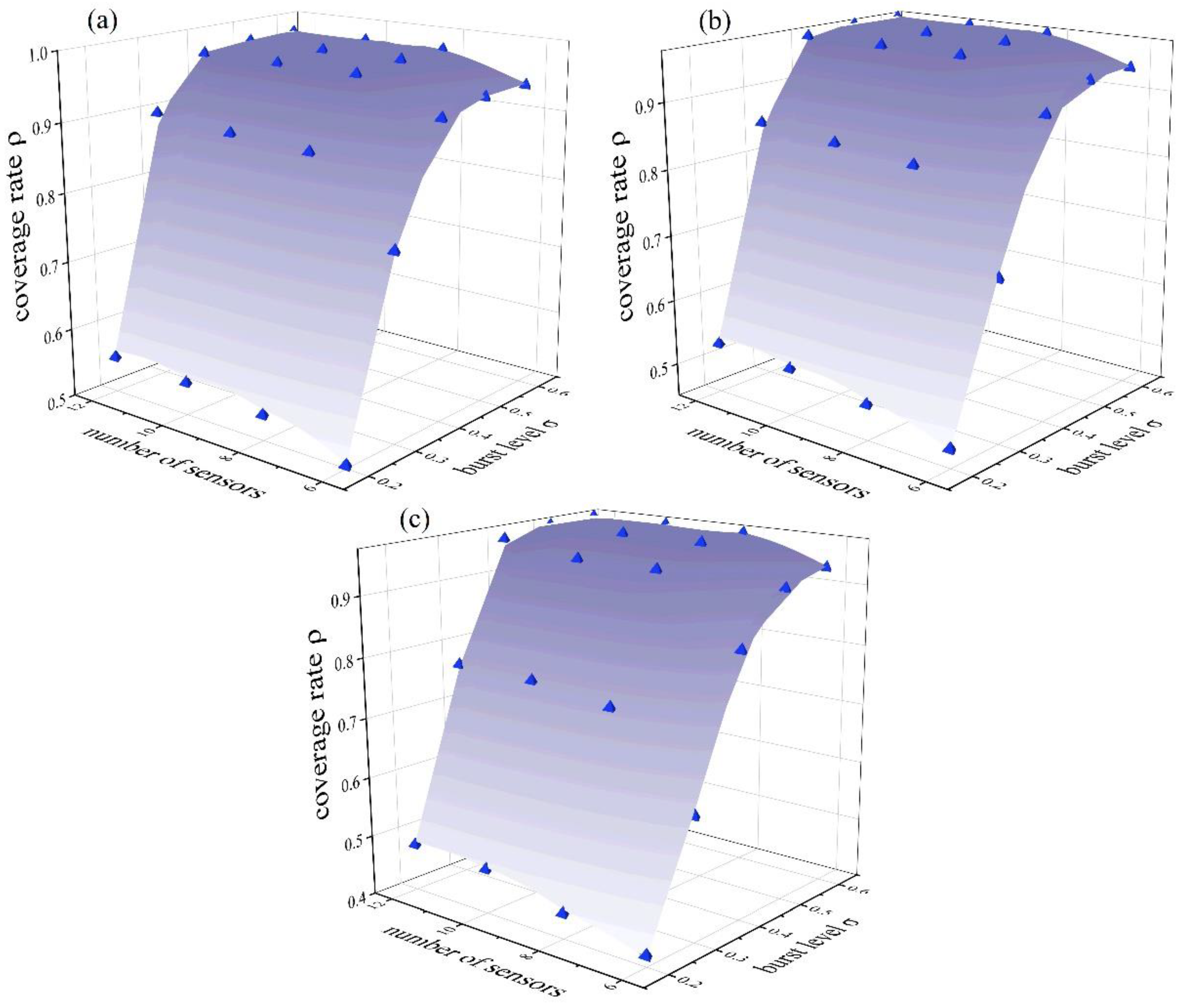
The pipe burst level σ was set at 0.2, 0.3, 0.4, 0.5, 0.6, and pipe burst time t was set at 14:00 p.m., 12:00 p.m., 1:00 a.m. (corresponding to average flow, maximum flow and minimum flow during one-day duration, respectively) to obtain the indicator tensor under 5 × 3 = 15 different operating conditions. The coverage rate of monitoring schemes with different number of monitors was calculated according to Equation (6), and the results are shown in Figure 10.

As shown in Figure 10, when the number of pressure sensors is fixed, the coverage rate of the monitoring system increases with the increase of the burst level σ, which means that the perception domain of each monitoring sensor is extended. However, when σ reaches a certain high level, limited by the number of sensors and the different distribution of monitoring schemes, nodes far away from the sensors, especially the nodes on the branches with small pipe diameters, are still undetected; thus, the coverage rate of the monitoring system tends to be flat for each monitoring scheme. Considering the coverage rate of the six sensors under the average flow conditions, for example, when σ increases from 0.2 to 0.3, the coverage rate increases from 0.50 to 0.76. However, when σ increases from 0.5 to 0.6, the coverage will only increase from 0.93 to 0.94.

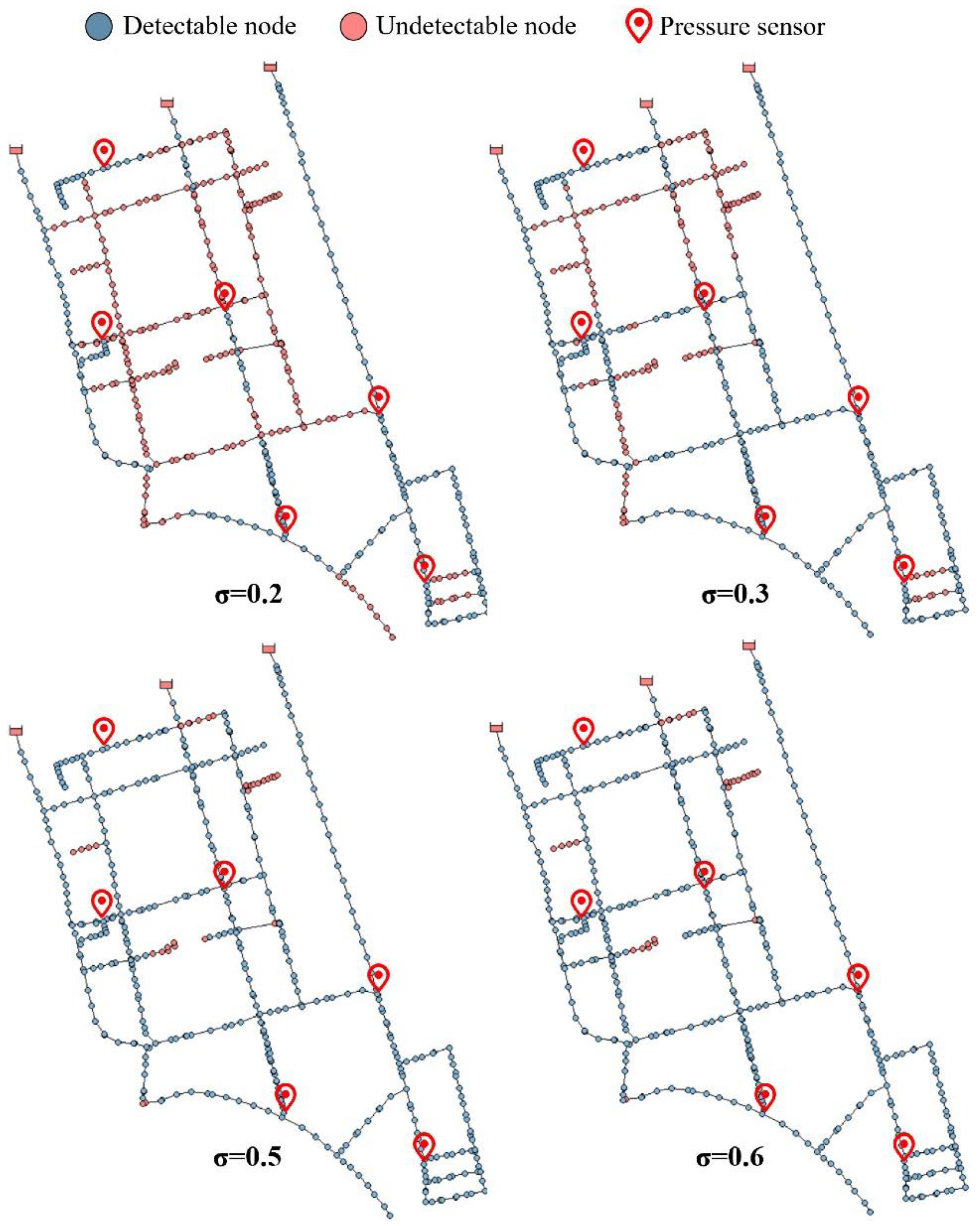
Figure 11 presents the coverage rate of the six sensors under different burst levels σ, and average flow conditions. When the burst level σ is 0.2, the monitoring system cannot sense the nodes in the middle branches, even if some points are close to the sensor. When the burst level σ increases to 0.3, most of the nodes with larger pipe diameters can be sensed. When the burst level σ increases to 0.5 or 0.6, except for several small-diameter branches distributed at the end of the pipe network, more than 93% of the nodes can be sensed by the pressure sensor.

Conversely, in case of a fixed level of pipe burst, as the number of pressure sensors increases, the coverage rate of the monitoring system will increase. However, when the number of sensors reaches a certain number, the coverage rate of the monitors will also increase. For example, under the average flow conditions, when the burst level σ is 0.3, the coverage rate of the six sensors is 0.76. When sensors increase to eight, the coverage rate increases to 0.87. When sensors increase to 12, the coverage rate also increases to 0.89.

We can also find that the coverage rate of the monitoring system is more sensitive to the change of pipe burst level than the change of sensor numbers. For example, in each monitoring scheme, when the pipe burst level increases from 0.2 to 0.3, the coverage rate increases 0.29 on average for different operating conditions. However, when the number of sensors increases from 6 to 12, at each pipe burst level, the coverage rate only increases 0.07 on average for different operating conditions. It provides us the strategy that during the process of monitoring system establishment, the monitoring accuracy target (the minimum level of pipe burst) should be determined first, and then the number of sensors can be reasonably assigned in the system accordingly.

Based on the calculation of the indicator tensor and the analysis of the coverage rate, the identification ability of the monitoring system can be analyzed under the conditions of a different number of sensors and different levels of pipe burst. This method provides an applicable framework of monitoring systems evaluation to the stakeholders of WSNs and helps them to quantitatively analyze the monitoring system corresponding to different operating conditions under certain cost (number of pressure sensors) constraints during the construction of the monitoring system. It can also help them quantitatively analyze and optimize the performance of existing monitoring systems.

4. Conclusions

In this paper, a framework of pressure sensor placement in WSNs was proposed based on Graph Neural Network algorithm. The SDCN algorithm was used to process hydraulic characteristics and topological structure characteristics for cluster analysis of WSNs. The network was divided into several partitions according to both hydraulic conditions similarity and topological connectivity of the WSN. Then, the sensitivity of pipe burst identification was analyzed by indicator tensor and partition perception rate calculation, and the node with the highest average partition perception rate was selected as the monitoring position in each partition. Case studies were conducted, and the proposed method was compared with classical K-means cluster method for pressure sensor placement. The key findings are summarized below:

(1) Experimental results show that SDCN algorithm can integrate topological and hydraulic characteristics of WSNs effectively. Based on monitoring partition establishment and partition perception rate analysis, the proposed method achieves a better monitoring scheme with more balanced distribution of sensors and higher coverage rate for pipe burst detection.

(2) When hydraulic condition changes, the monitoring system deployed with the proposed method is robust compared with K-means method, which shows that it is necessary to take multiple hydraulic conditions into consideration when arranging monitoring sensors.

(3) The coverage rate of the monitoring system is more sensitive to the change of pipe burst level than the change of sensor numbers. Thus, the monitoring accuracy target (minimum pipe burst level) should be determined first, and then the number of sensors can be reasonably assigned in the system accordingly.

(4) The proposed methodology facilitates the stakeholders of water supply systems to analyze the identification ability of monitoring systems under different operating conditions and economic constraints, which offers necessary and valuable guidance in the decision-making processes of the monitoring system establishment.

This paper uses nodal pressure to represent hydraulic characteristics, and the adjacency matrix of the WSN directed graph represents topological characteristics. In future research, we should consider introducing other hydraulic characteristics such as nodal demand and topological characteristics such as pipe diameter and pipe length, which will enhance topological feature presentation learning and improve the clustering effect of graph neural network analysis. Moreover, some important customers with little tolerance of water supply failure in the WSN should be covered in the perception domain during analysis process; thus, these places can be monitored effectively. At the same time, more complex hydraulic conditions, such as the scenarios of seasonal changes, system operation scheduling and water treatment plants switching, should be studied in the future.

References

- Azevedo, B.; Saurin, T.A. Losses in Water Distribution Systems: A Complexity Theory Perspective. Water Resour. Manag. 2018, 32, 1–18. [Google Scholar] [CrossRef]
- Frances-Chust, J.; Brentan, B.M.; Carpitella, S.; Izquierdo, J.; Montalvo, I. Optimal Placement of Pressure Sensors Using Fuzzy DEMATEL-Based Sensor Influence. Water 2020, 12, 493. [Google Scholar] [CrossRef] [Green Version]
- Meier, R.W.; Barkdoll, B.D. Sampling design for network model calibration using genetic algorithms. J. Water Resour. Plan. Manag. 2000, 126, 245–250. [Google Scholar] [CrossRef]
- Deschaetzen, W.; Walters, G.A.; Savic, D.A. Optimal sampling design for model calibration using shortest path, genetic and entropy algorithms. Urban Water 2000, 2, 141–152. [Google Scholar] [CrossRef]
- Kang, D.; Pasha, M.; Lansey, K. Approximate methods for uncertainty analysis of water distribution systems. Urban Water J. 2009, 6, 233–249. [Google Scholar] [CrossRef]
- Kang, D.; Lansey, K. Optimal Meter Placement for Water Distribution System State Estimation. J. Water Resour. Plan. Manag. 2010, 136, 337–347. [Google Scholar] [CrossRef]
- Zhou, X.; Tang, Z.; Xu, W.; Meng, F.; Chu, X.; Xin, K.; Fu, G. Deep learning identifies accurate burst locations in water distribution networks. Water Res. 2019, 166, 115058. [Google Scholar] [CrossRef]
- Cheng, W.; Chen, Y.; Xu, G. Optimizing Sensor Placement and Quantity for Pipe Burst Detection in a Water Distribution Network. J. Water Resour. Plan. Manag. 2020, 146, 04020088. [Google Scholar] [CrossRef]
- Sousa, J.; Ribeiro, L.; Muranho, J.; Marques, A.S. Locating Leaks in Water Distribution Networks with Simulated Annealing and Graph Theory. Procedia Eng. 2015, 119, 63–71. [Google Scholar] [CrossRef] [Green Version]
- Afsar, M.M.; Tayarani-N, M.-H. Clustering in sensor networks: A literature survey. J. Netw. Comput. Appl. 2014, 46, 198–226. [Google Scholar] [CrossRef]
- Jun, S.; Kwon, H.J. The Optimum Monitoring Location of Pressure in Water Distribution System. Water 2019, 11, 307. [Google Scholar] [CrossRef] [Green Version]
- Starczewska, D.; Collins, R.; Boxall, J. Transient Behavior in Complex Distribution Network: A Case Study. Procedia Eng. 2014, 70, 1582–1591. [Google Scholar] [CrossRef] [Green Version]
- Cheng, L.; Du, K.; Tu, J.P.; Dong, W.X. Optimal Placement of Pressure Sensors in Water Distribution System Based on Clustering Analysis of Pressure Sensitive Matrix. Procedia Eng. 2017, 186, 405–411. [Google Scholar] [CrossRef]
- Likas, A.; Vlassis, N.; Verbeek, J.J. The global k-means clustering algorithm. Pattern Recognit. 2003, 36, 451–461. [Google Scholar] [CrossRef] [Green Version]
- Wu, Y.; Liu, S.; Wu, X.; Liu, Y.; Guan, Y. Burst detection in district metering areas using a data driven clustering algorithm. Water Res. 2016, 100, 28–37. [Google Scholar] [CrossRef] [PubMed]
- Wang, J.; Sun, H. Optimal Algorithm of Pressure Measurement Node Layout in Water Distribution Network. J. Beijing Inst. Civ. Eng. Archit. 2005, 21, 51–54. [Google Scholar]
- Dong, L.; Xue, H.; Zhang, W. Optimal layout method of water pressure monitoring points for water supply network based on fault diagnosis. J. Civ. Archit. Environ. Eng. 2018, 40, 53–61. [Google Scholar]
- Farley, B.; Mounce, S.; Boxall, J. Field testing of an optimal sensor placement methodology for event detection in an urban water distribution network. Urban Water J. 2010, 7, 345–356. [Google Scholar] [CrossRef]
- Xu, K.; Hu, W.; Leskovec, J.; Jegelka, S. How powerful are graph neural networks? arXiv 2018, arXiv:1810.00826. [Google Scholar]
- Wu, Z.; Pan, S.; Chen, F.; Long, G.; Zhang, C.; Philip, S.Y. A comprehensive survey on graph neural networks. IEEE Trans. Neural Netw. Learn. Syst. 2020, 32, 4–24. [Google Scholar] [CrossRef] [PubMed] [Green Version]
- Bo, D.; Wang, X.; Shi, C.; Zhu, M.; Lu, E.; Cui, P. Structural deep clustering network. In Proceedings of the Web Conference, Taipei, Taiwan, 20–24 April 2020; pp. 1400–1410. [Google Scholar]
- Kipf, T.N.; Welling, M. Semi-supervised classification with graph convolutional networks. arXiv 2016, arXiv:1609.02907. [Google Scholar]
- Atwood, J.; Towsley, D. Diffusion-convolutional neural networks. In Proceedings of the Advances in Neural Information Processing Systems, Barcelona, Spain, 5–10 December 2016; pp. 1993–2001. [Google Scholar]
- Wagner, J.M.; Shamir, U.; Marks, D.H. Water distribution reliability: Simulation methods. J. Water Resour. Plan. Manag. 1988, 114, 276–294. [Google Scholar] [CrossRef] [Green Version]
- Kittel, T.; Heitzig, J.; Webster, K.; Kurths, J. Timing of transients: Quantifying reaching times and transient behavior in complex systems. New J. Phys. 2017, 19, 83005. [Google Scholar] [CrossRef]
- He, P.; Tao, T.; Xin, K.; Li, S.; Yan, H. Modelling Water Distribution Systems with Deficient Pressure: An Improved Iterative Methodology. Water Resour. Manag. 2016, 30, 593–606. [Google Scholar] [CrossRef]
- Lambert, A. What do we know about pressure: Leakage relationships in distribution systems? In Proceedings of the IWA System Approach to Leakage Control and Water Distribution Systems Management, Brno, Czech Republic, 16–18 May 2001. [Google Scholar]
Figure 1.
The framework of pressure sensor placement based on graph neural network clustering method.
Figure 2.
Monitoring partition establishment.
Figure 3.
Arrangement of monitoring sensors.
Figure 4.
The experimental model.
Figure 5.
Compassion of clustering results.
Figure 6.
The study water supply network.
Figure 7.
Pressure sensor arrangement using SDCN method.
Figure 8.
Pressure sensor arrangement for the K-means clustering approach.
Figure 9.
Coverage rates of different sensor placement schemes. The abscissa of the chart represents the level of pipe burst, the ordinate represents the coverage rate, the red curve represents the proposed method, and the blue curve represents the K-means clustering method. (a–c) represent the coverage rates of different monitoring schemes at average flow, maximum flow and minimum flow, respectively.
Figure 10.
Coverage rate of pressure sensors under different operating conditions. (a–c) represent the coverage rates at average flow, maximum flow and minimum flow, respectively.
Figure 11.
Detection results of six pressure sensors under average flow conditions.
Publisher’s Note: MDPI stays neutral with regard to jurisdictional claims in published maps and institutional affiliations. |
© 2022 by the authors. Licensee MDPI, Basel, Switzerland. This article is an open access article distributed under the terms and conditions of the Creative Commons Attribution (CC BY) license (https://creativecommons.org/licenses/by/4.0/).
Share and Cite
MDPI and ACS Style
Peng, S.; Cheng, J.; Wu, X.; Fang, X.; Wu, Q. Pressure Sensor Placement in Water Supply Network Based on Graph Neural Network Clustering Method. Water 2022, 14, 150. https://doi.org/10.3390/w14020150
AMA Style
Peng S, Cheng J, Wu X, Fang X, Wu Q. Pressure Sensor Placement in Water Supply Network Based on Graph Neural Network Clustering Method. Water. 2022; 14(2):150. https://doi.org/10.3390/w14020150
Chicago/Turabian StylePeng, Sen, Jing Cheng, Xingqi Wu, Xu Fang, and Qing Wu. 2022. "Pressure Sensor Placement in Water Supply Network Based on Graph Neural Network Clustering Method" Water 14, no. 2: 150. https://doi.org/10.3390/w14020150
Note that from the first issue of 2016, this journal uses article numbers instead of page numbers. See further details here.