Using Convolutional Neural Networks to Build a Lightweight Flood Height Prediction Model with Grad-Cam for the Selection of Key Grid Cells in Radar Echo Maps

Abstract

Recent climate change has brought extremely heavy rains and widescale flooding to many areas around the globe. However, previous flood prediction methods usually require a lot of computation to obtain the prediction results and impose a heavy burden on the unit cost of the prediction. This paper proposes the use of a deep learning model (DLM) to overcome these problems. We alleviated the high computational overhead of this approach by developing a novel framework for the construction of lightweight DLMs. The proposed scheme involves training a convolutional neural network (CNN) by using a radar echo map in conjunction with historical flood records at target sites and using Grad-Cam to extract key grid cells from these maps (representing regions with the greatest impact on flooding) for use as inputs in another DLM. Finally, we used real radar echo maps of five locations and the flood heights record to verify the validity of the method proposed in this paper. The experimental results show that our proposed lightweight model can achieve similar or even better prediction accuracy at all locations with only about 5~15% of the operation time and about 30~35% of the memory space of the CNN.

1. Introduction

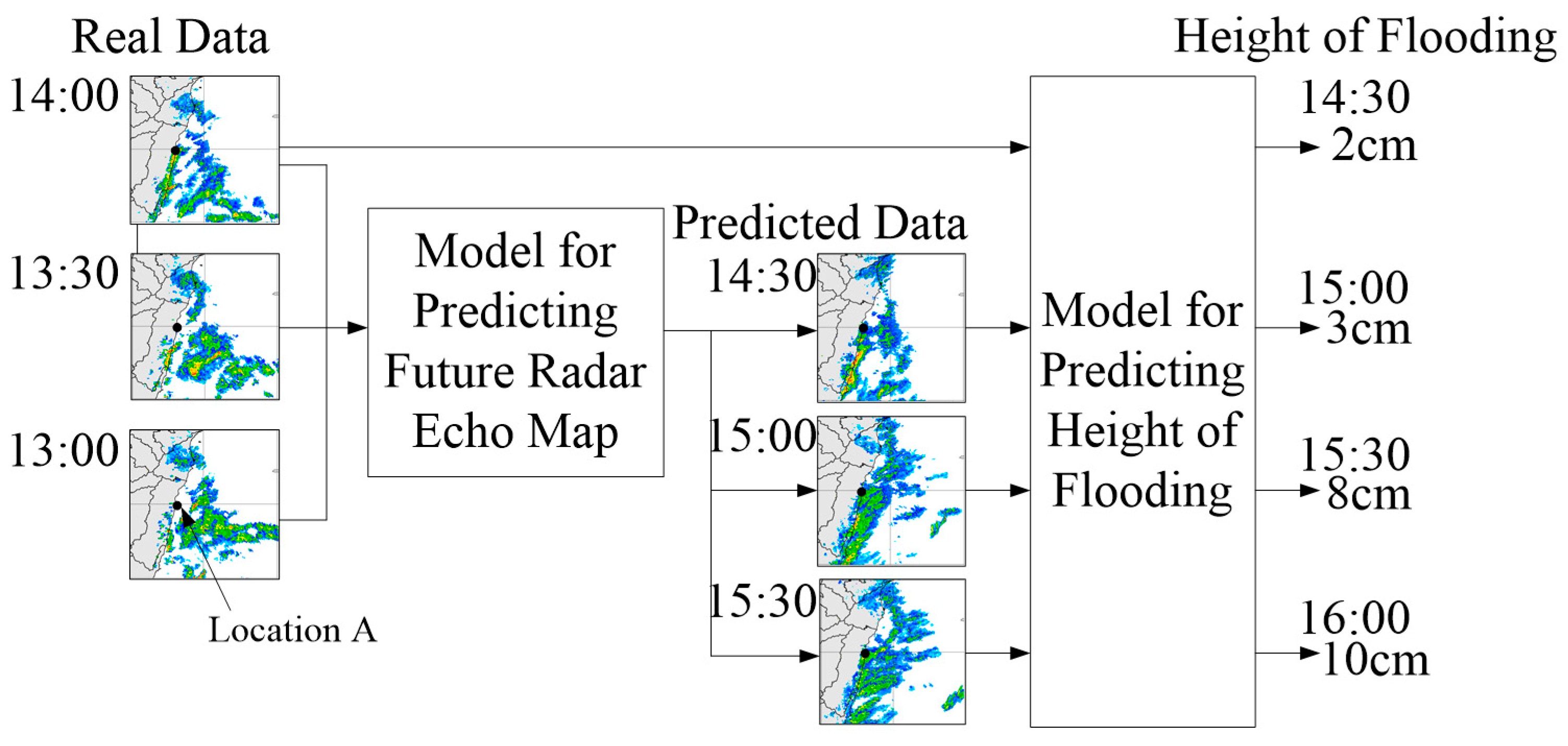
Recent changes in climatic conditions have increased the incidence of flooding worldwide. Flood warnings are based on the predicted height of the flood, and most previous research in flood height prediction has been based on radar echo maps and hydrological models [1,2,3]. Figure 1 illustrates the concept underlying this type of research. Suppose that the current time is 13:00, 1 January 2022, and the Central Weather Bureau has trained a model for location A. Using the radar echo map for time t as an input, the model outputs a prediction for the height of flooding at location A at time t + 30 min. In this way, it is possible to use radar echo maps from 13:00, 13:30, and 14:00 to simulate radar echo maps indicating the conditions predicted for 14:30, 15:00, and 15:30. Using the actual radar echo map from 14:00 and the predicted radar echo maps from 14:30 to 15:30 as inputs, it is then possible to predict the height of flooding in location A for every half hour between 14:30 and 16:00.

Scholars have developed a variety of hydrological models to illustrate the correlation between radar echo maps and flood height. Mecklenburg et al. [1] constructed a model to simulate radar echo maps for use in predicting flood height. Using the Hydrog model and data of two flood events in the Czech Republic, Šálek et al. [2] confirmed that radar echo maps can indeed be used to make accurate predictions pertaining to flood events. Novák et al. [3] demonstrated that tracking radar echoes via correlation-based quantitative forecasts of precipitation provide flood predictions of high accuracy. To improve the accuracy of flood predictions, Yoon [4] developed a blending model involving six commonly used quantitative precipitation forecasts as inputs for the StormWater Management Model and Grid-based Inundation Analysis Model.

The methods outlined above have no doubt proven effective in the prediction of flooding events; however, they have two notable shortcomings: (1) Establishing hydrological models requires considerable professional knowledge and extensive measurement data, and updating can only be performed by teams of highly specialized individuals. Most scholars are unable to acquire and/or apply the data or verify the correctness of their predictions. (2) Collecting all of the data required to make flood height predictions for all locations would require considerable time and increase the likelihood that important factors are inadvertently overlooked.

Many scholars have begun applying deep learning models (DLMs) to radar echo maps. Chen et al. [5] developed an extended model based on convolutional long short-term memory to predict future radar echo maps. Yin et al. [6] used DLMs to fill occluded areas in radar echo maps. Singh et al. [7] modified part of the long short-term memory structure to enable high-precision precipitation nowcasting using radar echo maps. Yin et al. [8] performed high-precision strong convection nowcasting based on the convolutional gated recurrent unit. Yan et al. [9] used a dual-channel neural network to make short-term predictions of precipitation. Previous experience indicates that DLMs have two fundamental benefits: (1) DLMs do not require professional knowledge and depend entirely on historical data, such that the building and updating process is relatively simple. (2) DLMs automate the process of finding patterns in inputs and outputs, thereby making it possible to obtain a more comprehensive collection of factors (far exceeding what can be achieved using conventional approaches) with a corresponding increase in accuracy. To the best of our knowledge, this is the first paper to address the use of radar echo maps and DLMs for the prediction of flood height.

It should be noted that using CNNs to formulate flood height predictions directly from radar echo maps would be highly inefficient. Discrete CNNs would be required to deal with the flood conditions specific to every site within large regions or the entire country. Furthermore, CNN operations would have to be completed in short intervals (e.g., 10 min or 1 h), thereby necessitating the use of expensive high-end servers. Our primary objective in the current study was to reduce the cost of operating DLMs without undermining prediction accuracy.

Previous attempts to reduce the operating cost of DLMs can be divided into two approaches: (1) methods aimed at simplifying the model structure while maintaining the dimensions of the input data, and (2) methods aimed at reducing the input dimensions without simplifying the model structure. The first approach reduces computational cost by deleting the layers, neurons, or weights that contribute least to the output. Han et al. [10] deleted weight values and Li et al. [11] deleted entire filter layers. Molchanov et al. [12] used the Taylor expansion to explore the influence of each filter layer on the loss function in order to identify filter layers for deletion. Luo et al. [13] implemented a similar approach using a greedy algorithm. Note that the first approach is effective in reducing the computational cost of DLMs; however, a lack of compatibility with many graphics processing units means that this approach is ill-suited to many practical online applications. The second approach involves training a DLM and then disassembling it to obtain key factors for use as inputs for machine learning models or deep learning models with limited input dimensionality. The fact that these models employ only the most important factors for modeling means that their prediction accuracy does not deviate considerably from that of the original DLM. In the scheme proposed by Sani et al. [14], the key factors are contained in the output of the last pooling layer after training. Mohammad et al. [15] developed a set of mathematical theories by which to disassemble the trained DLM to obtain the key factors. These studies confirmed that the key factors identified by the DLM could be used to perform high-precision motion recognition using a low-cost model. Chen and Lee [16] pointed out that the use of complex mathematical conversion is a waste of computational resources. They developed a radius base function long short-term memory model to simplify the disassembly process. Furthermore, the key factors selected using their method match the input of the original model, thereby eliminating the extra step of converting model inputs into key factors. They went on to demonstrate that their key factors could be used to achieve prediction accuracy on par that of deep learning from any machine learning model, with presumably far lower computational overhead.

In the current study, we adopted an approach similar to the scheme described in [16]. Briefly, a DLM is trained using a radar echo map as the input and flood height as the output. From the trained DLM, key grid cells are extracted (i.e., key factors in [16]) for use as inputs in other lightweight models. Finally, only the lightweight models are used in online applications in order to reduce the computational cost. Figure 2 presents a flow chart of the proposed scheme. Note that even when using the proposed scheme to make flood predictions for a large number of locations simultaneously, the computational demands are far lower than those imposed by a DLM. Note also that this approach greatly increases the cost of building lightweight models; however, we disregarded the cost of model building due to the fact that model rebuilding or updating is required only for long-term predictions (quarterly or yearly). The methods outlined in [16] are inapplicable to our scheme, because the model input in that study is an independent data dimension, whereas the model input in this study is a radar echo map divided into a grid with strong dependence among adjacent grid cells.

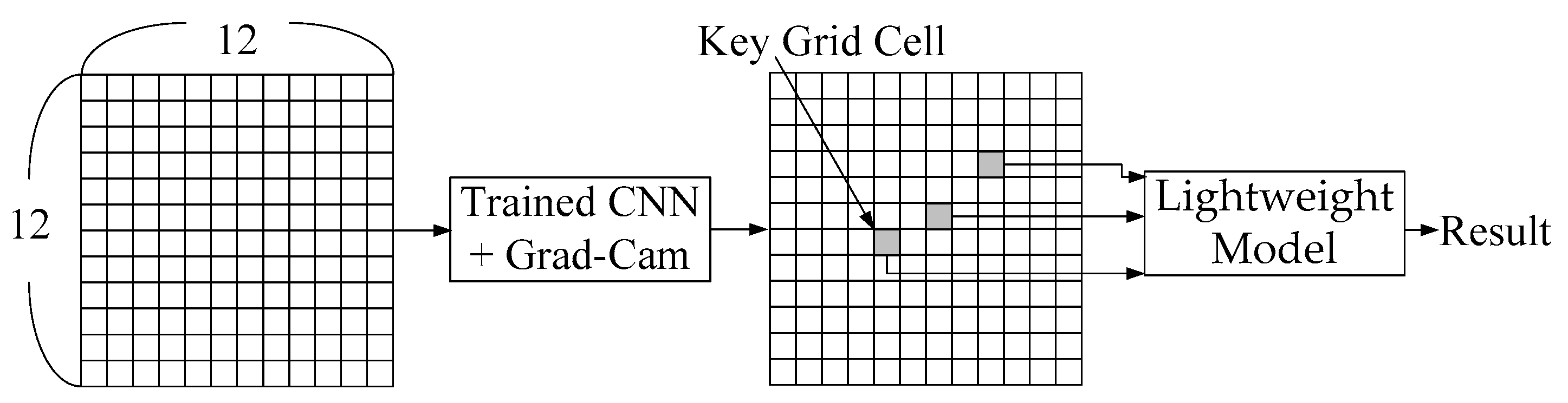
In the current study, we employed a convolutional neural network (CNN) in conjunction with the Grad-Cam package for the extraction of key grid cells from radar echo maps (representing regions with the greatest impact on flooding) for use as inputs into another DLM, as shown in Figure 2. This approach makes it possible to reduce the number of input dimensions with a corresponding reduction in computational overhead. This, in turn, should make it possible to make multiple simultaneous predictions of flood height over large areas. Note that we selected a CNN for this research because the model input is a radar echo map comprising a large number of grid cells, and the model output is a single value (flood height) associated with the target place. CNNs are among the most effective models for predicting single output values from grid input data. After inputting data (in grid format) into the trained CNN, back propagation is used to identify the key cells (i.e., those of greatest relevance of the output value). The Grad-Cam package is an accessory widely used with CNNs. He et al. [17] used a CNN with Grad-Cam to select factors that are important in the detection of lung cancer. Li et al. [18] used Grad-Cam to optimize channel selection in a CNN for EEG-based intention recognition. Marsot et al. [19] combined a CNN with Grad-Cam to optimize facial recognition in a porcine model. Combining a CNN with Grad-Cam is a reasonable approach to analyzing radar echo maps; however, our grid input differs fundamentally from the inputs in previous papers. The grid cells in this paper represent distinct geographic locations, which do not vary. The grid inputs in most previous studies were derived from images, such that the entity represented by the grid cell tended to vary. Thus, we had to modify the means by which Grad-Cam is used for the extraction of key factors. In the end of this work, we will conduct experiments using actual radar echo maps and historical flooding records to confirm that the proposed CNN–Grad-Cam framework can indeed identify the grid cells with the greatest influence on flood heights in multiple locations. Our results confirmed that using only the key grid cells to build a DLM reduced computational overhead, while maintaining accuracy close to that of the original CNN.

The fact that our model is based primarily on the key features of DLM means that as long as relevant inputs are available, a lightweight model can be established without the need for hydrological knowledge. However, this type of system cannot be used when input–output correlation is poor, when all input dimensions that affect the output value are unavailable, or when the reproducibility of historical data is not good. In real-world scenarios, flood height can be affected by other factors, such as the tides, upstream rainfall, and flood discharge from reservoirs. In such situations, the exclusive use of radar echo maps would be unlikely to achieve accurate predictions in areas adjacent to the sea or rivers. Additionally, when flood conditions in low-lying areas are controlled by pumps, DLM cannot be used to establish an effective predictive model, let alone a lightweight model. Therefore, we recommend applying the proposed model to relatively simple environments, such as places where the flooding situation is predominantly affected by rainfall or terrain. Note that such environments are very common in most rural and even urban locations. In this paper, we consider only the relationship between radar echo maps and flood height, such that the CNN is used primarily for first-stage modeling. CNNs provide good modeling results when using data in a grid format (e.g., a map grid), but poor modeling results when grid-format data and single data are input together. In the future, we will develop extended versions of this model to overcome the limitations of conventional CNNs.

Section 2 presents an overview of the relevant literature. The proposed algorithm is presented in Section 3. Simulation experiments are outlined in Section 4. Conclusions and future work are discussed in Section 5.

2. Related Works

This section presents an overview of previous studies on the two research topics related to this thesis: flood prediction methods and the application of Grad-Cam.

2.1. Flood Prediction

Researchers have developed a wide range of methods by which to investigate extreme weather and flooding, including hydrological models, statistical methods, machine learning schemes, and composite approaches. In their hydrological model, Thorndahl et al. [20] used weather radar data with various spatial and temporal resolutions to make rainfall predictions for use in urban flood models aimed at predicting the scale of flooding. To improve the accuracy of flood predictions, Yoon [4] developed a blending model using five quantitative precipitation forecasts to predict rainfall, including MAPLE, KONOS, SCDM, UM LDAPS, and ASAPS. In their system, rainfall is used as an input, and the StormWater Management Model and Grid-based Inundation Analysis Model are used to make predictions pertaining to flooding in urban areas.

Wang et al. [21] adopted a statistical approach, in which a city is divided into a grid and a linear programming model is used to explore the flow of water in and out of the grid cells to facilitate flood predictions in real-time. Jati et al. [22] identified six key factors for use in logistic regression to predict floods, resulting in prediction accuracy of roughly 85–95%.

Berkhahn et al. [23] used machine learning to create a physical model for use in generating artificial flood events, the maximum flood level of which was estimated using an ANN. A combination of adaptive neuro fuzzy inference with a genetic algorithm, differential evolution, and particle swarm optimization allowed Arora et al. [24] to achieve results superior to any single model or other combined models. SyedKabir et al. [25] used a 2D hydraulic model to generate simulation data and a CNN model for training. Comparisons with actual flood events verified that their CNN model was superior to support vector regression in predicting the maximum submerged area and depth.

The composite ARMT system developed by Hsu et al. [26] uses weather radar to predict the area of rainfall, after which a closed-circuit television system is used to collect images depicting rainfall to estimate local flooding. In comparison with historical data, their method achieved accuracy of 83–92%. Ichim and Popescu [27] combined aerial drone images with a CNN model to identify instances of flooding in rural areas.

2.2. Related Research on Grad-Cam

The core concept underlying the Grad-CAM scheme is simple. Regardless of the type of neural network implemented after the convolutional layer, it should be possible to obtain weight values of features in the DLM (without modifying the model) for use in deriving key feature points. This method involves deriving gradient information from the last convolutional layer via back propagation, determining the importance of each neuron, and then generating a hot-zone map indicating the degree to which the CNN output is applicable to a given area. The fact that this method can be used to identify the area of interest in real-world applications means that the DLM does not need to be modified or retrained.

Numerous scholars have applied this method to image recognition tasks with the aim of enhancing the interpretability of the DLM and building a lightweight model that is easy to apply. Hata et al. [28] used DLM and electrocardiogram images to classify aortic valve stenosis. The use of Grad-CAM to find the key feature regions improved classification results. Chueh et al. [29] applied a DLM to retina OCT images in order to differentiate between males and females, whereupon Grad-CAM was used to identify gender-related retinal features. Panwar et al. [30] employed Grad-Cam in their CNN model for use in analyzing CXR and CT-Scan images of the lungs to detect COVID-19. They achieved accuracy of 95.61%, and the resulting heat maps greatly enhanced the interpretability of the results. Seerala et al. [31] used Grad-CAM to identify key features within chest X-ray images from pneumonia patients. Marsot et al. [19] used class activation maps generated by Grad-CAM to intuitively understand how a neural network model learns to distinguish parameters for animal classification. He et al. [17] used Grad-CAM to identify features of importance in predicting postoperative complications in cases of lung cancer. Grad-Cam technology has been widely used in image processing; however, this is the first study in which it is used for map analysis.

3. Algorithms

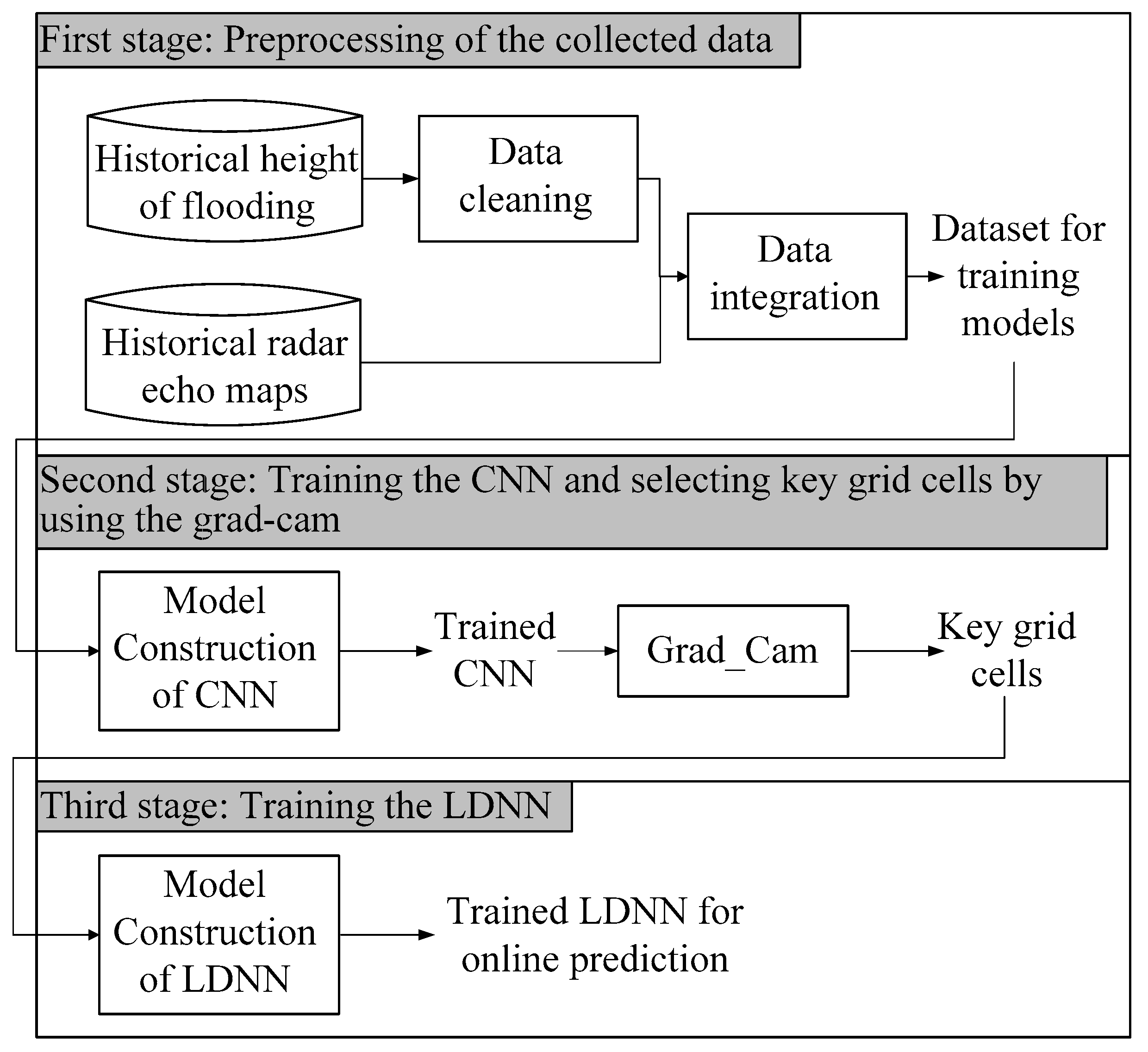
Figure 3 illustrates the three-stage computational framework proposed in this paper. Our aim is to predict the flood height in grid cell A. The first stage involves data pre-processing, aimed at sorting out the historical flood records pertaining to cell A and finding the radar echo map for the corresponding time point. The second stage involves training a CNN using the radar echo map identified in the previous stage (as the input) and the flood height of A (as the output). After training the CNN, Grad-Cam is used to find the grid cells that are key to estimating flood height in area A. The final stage involves using the key grid cells as input into a lightweight deep neural network (LDNN) for modeling and prediction. In the following subsection, we discuss the collection, cleaning, and integration of flood-related data and radar echo maps. We then introduce the CNN architecture, after which we describe how Grad-Cam is used to identify key grid cells. In the final subsection, we introduce the LDNN used in this paper.

3.1. Collection, Cleaning, and Integration of Flood-Related Data and Radar Echo Maps

In this section, we introduce the methods used in the collection and formatting of flood-related data. We also introduce the radar echo maps and discuss the means by which the data are assembled into a data set applicable to the CNN. Flood-related data from sensors is returned as a value representing the flood height at steady intervals. Assuming that the sensor is set up in grid cell A, the first time the sensor collects data is t₁, and a value is returned after every interval t. We then represent the flood height value of n consecutive returns as H_A = [h_A(t₁), h_A(t₂), …, h_A(t_n)], where t_i = t_i−1 + t. The value of t ranges from 10 min to 12 h. Due to network instability, external sensors are prone to missing H_A values. Cleaning and augmenting H_A values involves two sub-steps. The first sub-step involves obtaining a reasonable range of flood heights for grid cell A, based on historical data from the weather bureau. We then check whether the H_A values fall within that range, and mark any missing values or values outside that range. The second sub-step involves determining whether to change or discard the marked values, based on the timespan to the previous sub-step. If the duration of the marked value is less than 24 h, then Equation (1) is used to fill in the value in accordance with the situation at that time of day.

$$h_a(a+c){=h}_a(a)+\frac{c}{b+1}(h_a(a+b+1)-h_a(a\left)\right),$$

(1)

where a represents the time of the previous marked value, b represents the number of consecutively marked values, and c represents the data inserted for the cth record. If the duration of the marked value exceeds 24 h, then the marked value is simply discarded. If the inserted values for periods t₂ and t₃ in area A are h_A(t₂)′ and h_A(t₃)′, and the values within t₂₀ to t₄₀ are discarded, then the new H_A can be expressed as H_A′ = [h_A(t₁), h_A(t₂)′, h_A(t₃)′, h_A(t₄), …, h_A(t₁₉), h_A(t₄₁), …, h_A(t_n)].

After sorting out flood data for area A, we sort out the radar echo maps surrounding area A, which are usually obtained from the weather bureau. Assuming that the radar echo maps provided by the bureau are recorded at intervals of k, we obtain radar echo map data of the surrounding x × y grid with A as the center. Assuming that the time of the first radar echo map is k₁, and the interval between each image is k, then we can represent m continuous radar echo maps as P_A = [p_A(k₁), p_A(k₂), …, p_A(k_m)], where k_i = k_i−1 + k. The value of k usually ranges from 10 min to one hour. 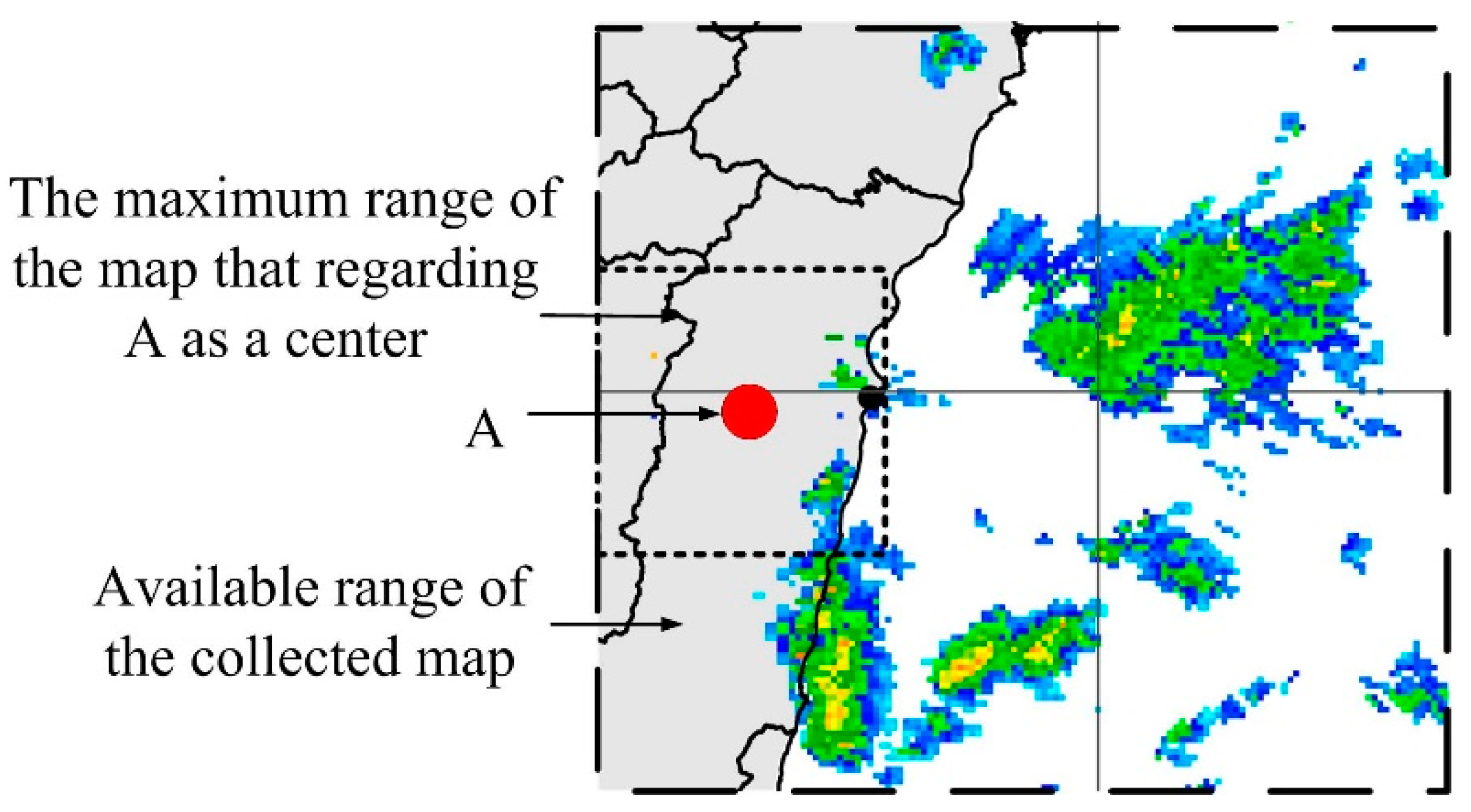The k_ith radar echo map p_A(k_i) in P_A can be expressed as p_A(k_i) = [v_a,ki(1, 1), v_a,ki(1, 2), …, v_a,ki(1, y), v_a,ki(2, 1), …, v_a,ki(2, y), …, v_a,ki(x, 1), …, v_a,ki(x, y)]. Note that A will not be in the center of the radar echo map when A is located at the edge of the map. 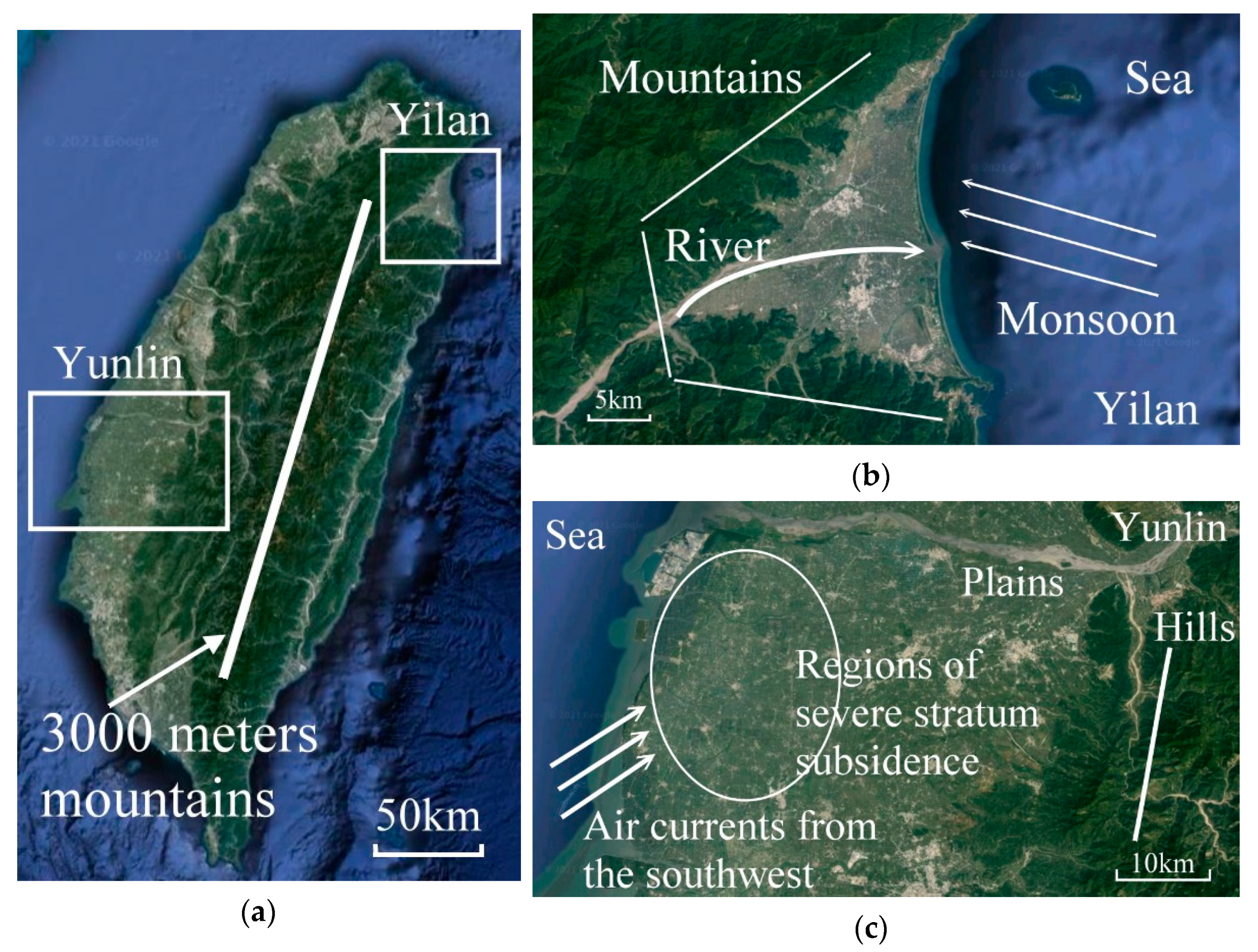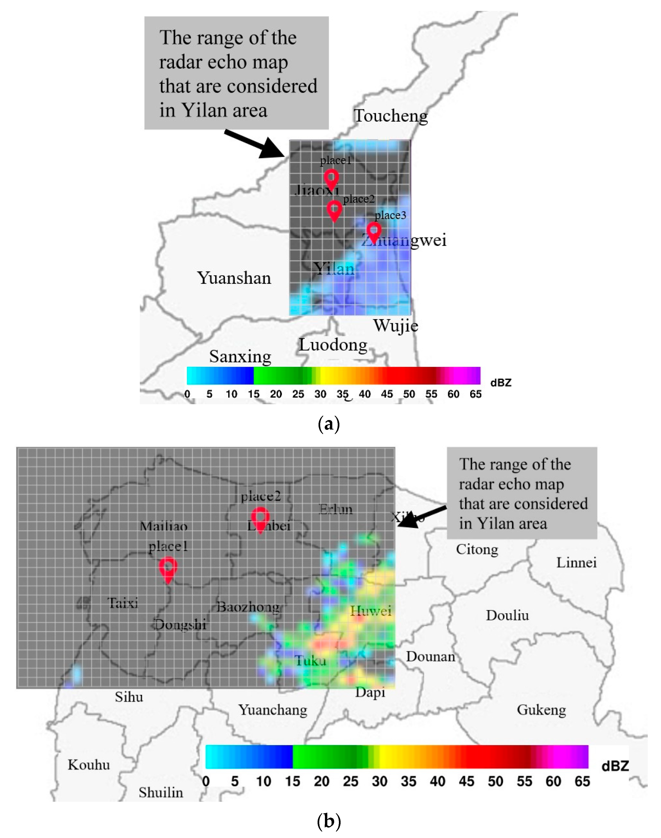In this situation, making A the center would limit the range of the radar echo map, as shown in Figure 4. Note also that the radar echo map grid is actually a rectangle, due to the limited the range of the radar echo map obtained from the government and limitations due to terrain and other factors. We must assume that the radar echo map obtained from the weather bureau is accurate and reasonable. The grid used for radar echo maps should be adjusted to the specifics of the intended application. The additional information provided by grids of high resolution can significantly increase CNN prediction accuracy, and our lightweight model based on the CNN architecture would also benefit from grid of higher resolution. Nonetheless, any improvement in accuracy would come at the cost of higher computational overhead. In other words, selecting the resolution of radar echo maps involves a trade-off between accuracy and computational capacity or efficiency. In fact, the computational demands of large-scale CNNs are likely to exceed the capacity of all but the most highly enabled computer systems.

Flood-related data and the radar echo map must be organized within a data set applicable to the CNN. This is achieved in two sub-steps: (1) Selection of flood and non-flood events, and (2) Combination of the event and the radar echo map. Sub-step (1) involves sorting through events one-by-one. Due to the rarity of flood events, most of the values in flood height data set H_A′ are 0 (i.e., only rare flood events are greater than 0). Inputting H_A′ directly into the CNN for training would result in data imbalance and corresponding inaccuracies. This situation can be avoided by balancing the ratio of non-flood events against flood events. We begin by recording the number of times the flood height value exceeded σ, where σ is the threshold value indicating a flood event, as defined by the government. We estimate the distribution of flood height levels, randomly select φ data points from the remaining non-flood events, and record when those data points occurred. For convenience, we assume that w pieces of data in H_A′ are retrieved. Note that the newly retrieved data are expressed as H_A″ = [h_A(tr₁)″, h_A(tr₂)″, …, h_A(tr_w)″]. The times associated with these data points are Time_A = {tr₁, tr₂, …, tr_w}, where tr₁, tr₂, …, tr_w are sorted chronologically but may be discontinuous.

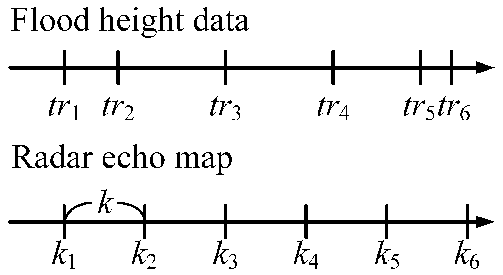
Sub-step (2) involves combining the data of flood height and the radar echo map. This sub-step is needed because the time intervals and time of the flood sensor and the radar echo map may be different. There is no direct correspondence, as shown in Figure 5. The details of this sub-step are as follows. We assume that the radar echo map data set is P_A = [p_A(k₁), p_A(k₂), …, p_A(k_m)], where k₁, k₂, …, k_m are continuous points in time, and the intervals between each point in time are k. We perform the following checks for the ith time point tr_i of Time_A.

Case 1: If there is a time point k_j in k₁, k₂, …, k_m that precisely matches tr_i, then we combine the k_jth radar echo map p_A(k_j) with flood height h_A(tr_i)″ as a single set of inputs and outputs.

Case 2: If there is no time point in k₁, k₂, …, k_m that matches tr_i, and the time interval between tr_i and tr_i+1 is greater than k, then we find k_j, the point in k₁, k₂, …, k_m closest to tr_i. We take the radar echo map p_A(k_j) of k_j and flood height h_A(tr_i)″ and combine them into a single set of inputs and outputs.

Case 3: If there is no time point in k₁, k₂, …, k_m that matches tr_i, and the time interval between tr_i and tr_i+1 is less than k, we find k_j, the point in k₁, k₂, …, k_m closest to tr_i. We take the radar echo map p_A(k_j) of k_j and flood height h_A(tr_i)’’ and combine them into a single set of inputs and outputs. Note that tr_i+1 and h_A(tr_i+1)’’ are not considered in subsequent calculations.

After checking all w time points in Time_A, we obtain a set that can be used as the input and output for the subsequent CNN [(p_A(tcnn₁), h_A(tcnn₁)″), (p_A(tcnn₂), h_A(tcnn₂)″), …, (p_A(tcnn_w′), h_A(tcnn_w′)″)], where tcnn_i represents the ith data in this set, and w′ is the total number of data points in the set (i.e., w′ < w).

3.2. CNN Architecture Used in Target Framework

In this section, we introduce the input, output, and network architecture of the proposed CNN. As described in the previous section, the ith input data of the CNN is p_A(tcnn_i) in CNN_IO, which represents a radar echo map with a grid size of α × β × γ, where β and γ represent the size of the radar echo map, and α indicates the number of characteristics of the radar echo map. The ith output data of the CNN is h_A(tcnn_i) in CNN_IO, which represents the flood height. As for the selection of CNN training, testing, and validation datasets, we recommend that the ratio should be set at 70%, 15%, 15% or 70%, 10%, 20% to meet most CNN training procedures. In addition, in order to maintain the independence of the three datasets, we suggest that the training, testing, and validation datasets be divided into different flooding events or into different flood years when the user has enough data.

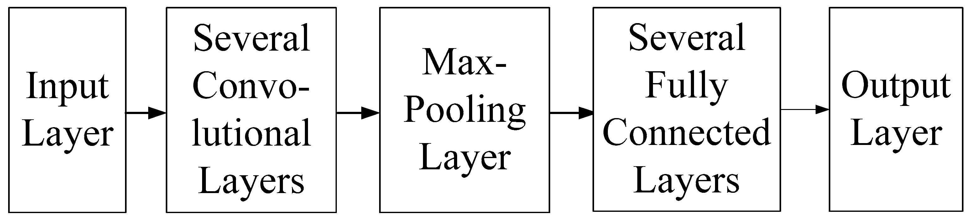
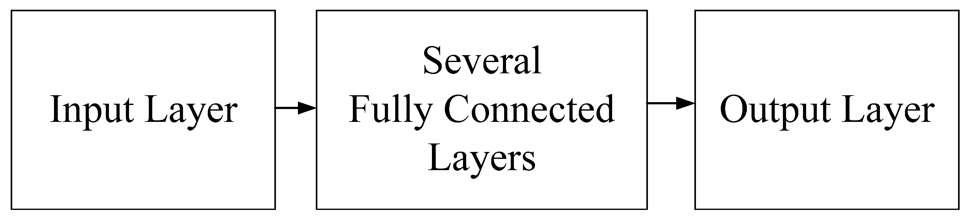
The internal architecture of the CNN used in this framework comprises an input layer, several convolutional layers, a max pooling layer, multiple fully connected layers, and an output layer, as shown in Figure 6. The mathematical formula of each layer and its physical meaning in flood height prediction are described below. The input layer is used to transfer the radar echo map into the model. The mathematical formula of any neuron in this layer can be expressed as follows:

O_z,x,y = p_A(tcnn_t)_z,x,y,

(2)

where O_z,x,y is the output value of the neuron with the zth feature located at (x, y). The multi-layer convolutional layer is used mainly to extract features from the radar echo map. Assuming that the size of the radar echo map received by the CNN is x × y and the CNN uses a total of n convolutional layers, we recommend setting the filter size of the first convolutional layer in accordance with the ratio of x to y. We do this because the rectangular data input of this CNN should be transformed into a square to facilitate subsequent processing. The filter size in the second convolutional layer is based on the output size of the previous layer. The number of convolutional layers depends on the size of the input radar echo map. Regardless of the convolutional layer in which a neuron is located, it can be expressed using the following mathematical formula:

$$O_{(z,x,y)}^i=act({\displaystyle {\sum }_{g=1}^s{\displaystyle {\sum }_{h=1}^s{l}_k^i{I}_{\left(z,x+g-1,y+h-1\right)}+b_k^i}}),$$

(3)

where oⁱ_(z,x,y) is the output value of the ith neuron whose zth feature is located at (x, y). bⁱ_k and lⁱ_k are, respectively, the corresponding bias vector and kernel in the layer. I_{(•,•,•)} is the input for this layer, and act(•)is the Relu activation function.

After the convolutional layer processes the radar echo map, a max-pooling layer is used to reduce the model size and highlight the important characteristics in the feature space. If the input data of a neuron in this layer is (C_i, R_i, H_i), then the output result is (C₀, R₀, H₀), the pool size of this layer is (p, p), and stride is s, such that the mathematical formula of the neuron can be written as

$$C_0=\lfloor \frac{C_i-p}{s}+1\rfloor ,$$

(4)

$$R_0=\lfloor \frac{R_i-p}{s}+1\rfloor ,$$

(5)

H₀ = H_i

(6)

After obtaining the results of the max-pooling layer, we use a multi-layer fully connected layer to model the connections between the important radar echo map features and the output flood height. The first layer of the fully connected layers begins by flattening the results of the max-pooling layer. Assuming that the result of the max-pooling layer is matrix (C_i, R_i, H_i), then the input of the first fully connected layer will be a vector of length C_i × R_i × H_i. Each neuron in these fully connected layers can be expressed using the following formula:

$$O_i=\sigma ({\displaystyle {\sum }_{j=1}^D{w}_{ij}}{I}_j)+bia{s}_i,$$

(7)

where o_i represents the output of the ith node, D represents the number of input features, I_j represents the feature input value from the jth node, w_ij is the weight from the jth node of the input to the ith node of the output, bias_i is the the offset vector of the ith node of the output, and σ(•) is a sigmoid function.

Following completion of multi-layer fully connected layer calculations, the flood height prediction is output by the output layer, which uses only one neuron fully connected to the last neuron in the fully connected layer. The mathematical formula of the neuron in the output layer can be written as follows:

$$o_j=\sigma (w_{ij}{i}_i)+b_j,$$

(8)

where o_j represents the output of a given node, σ(•) is the sigmoid function, and w_ij and b_j, respectively, indicate the corresponding weights and bias vectors.

3.3. Using Grad-Cam to Identify Key Grid Cells

This section explains the use of Grad-Cam to identify key grid cells to be marked by the CNN on the radar echo map for the prediction of flood height at the target location. We first introduce the operational concepts and formulas of Grad-Cam, and then introduce how Grad-Cam results can be used to identify key grid cells.

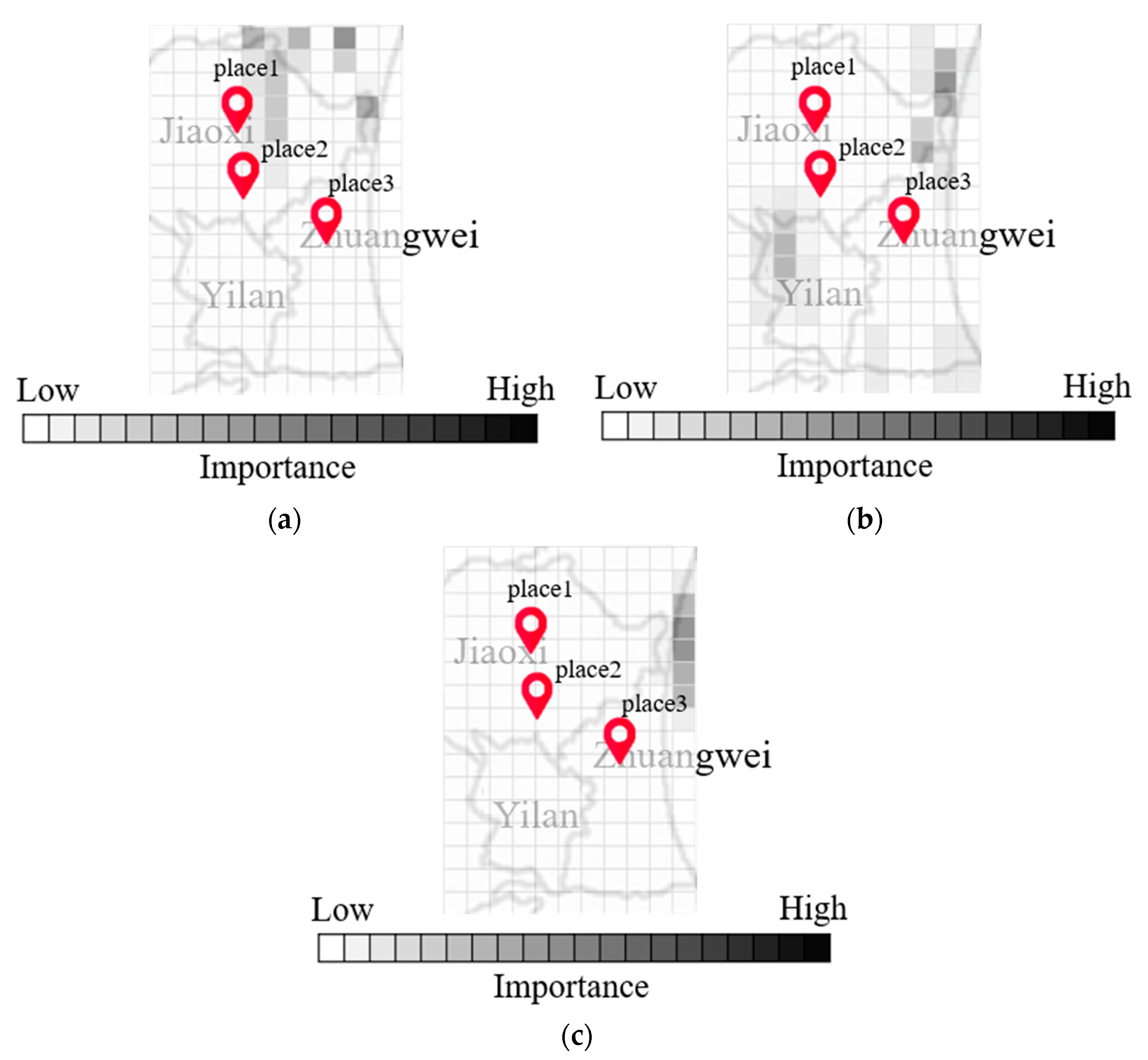
Generally speaking, after training a CNN and inputting data of the ith grid, the CNN result is based on the ith input. The Grad-Cam package uses gradient information of the previous convolutional layer in this CNN operation to infer the degree to which each cell of the ith input influences the ith output. A matrix is used to represent the degree of influence, and the size of the matrix is equal to the length and width of the input data. Scholars commonly represent this matrix using a heat map to make it easier to understand. 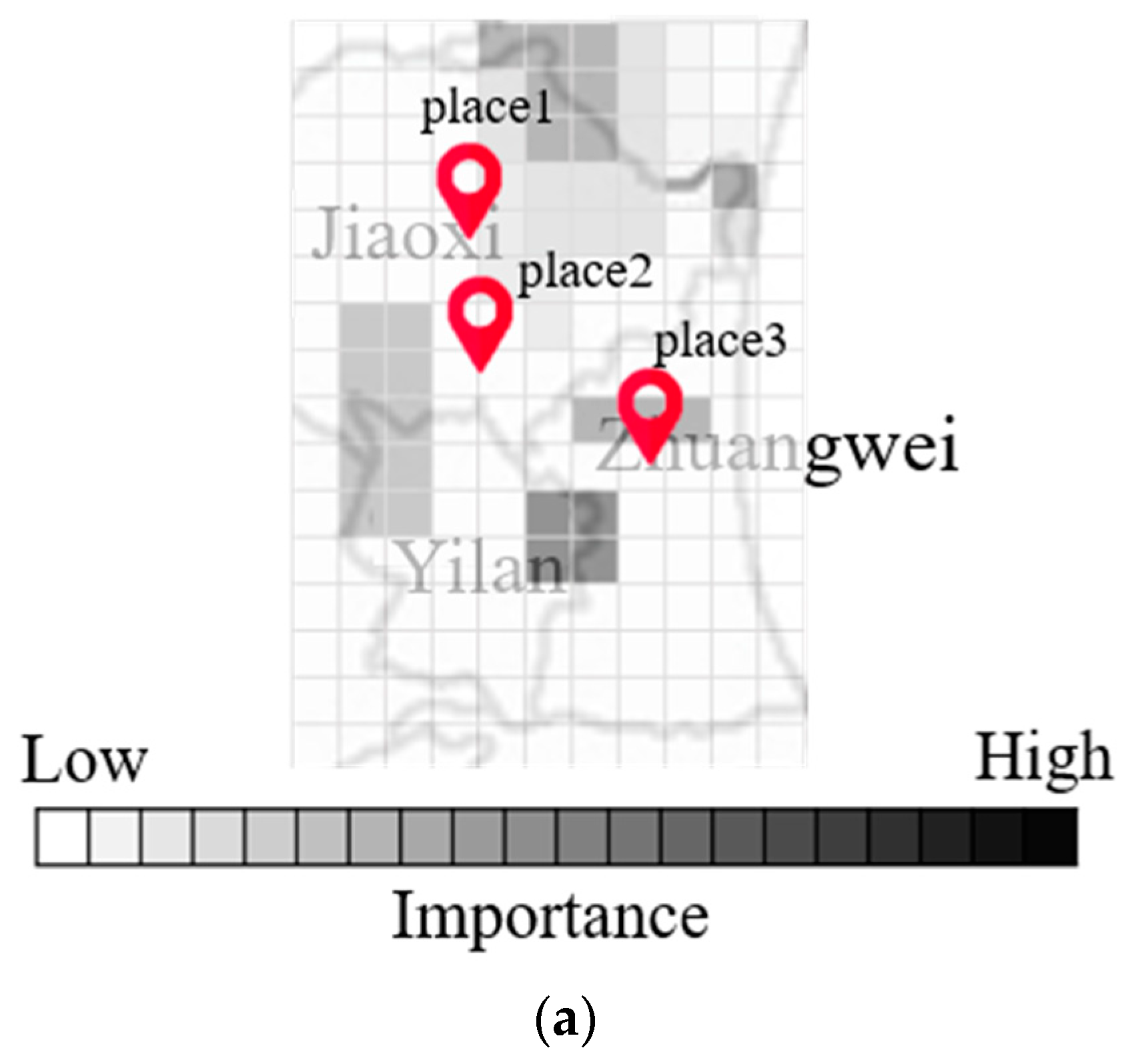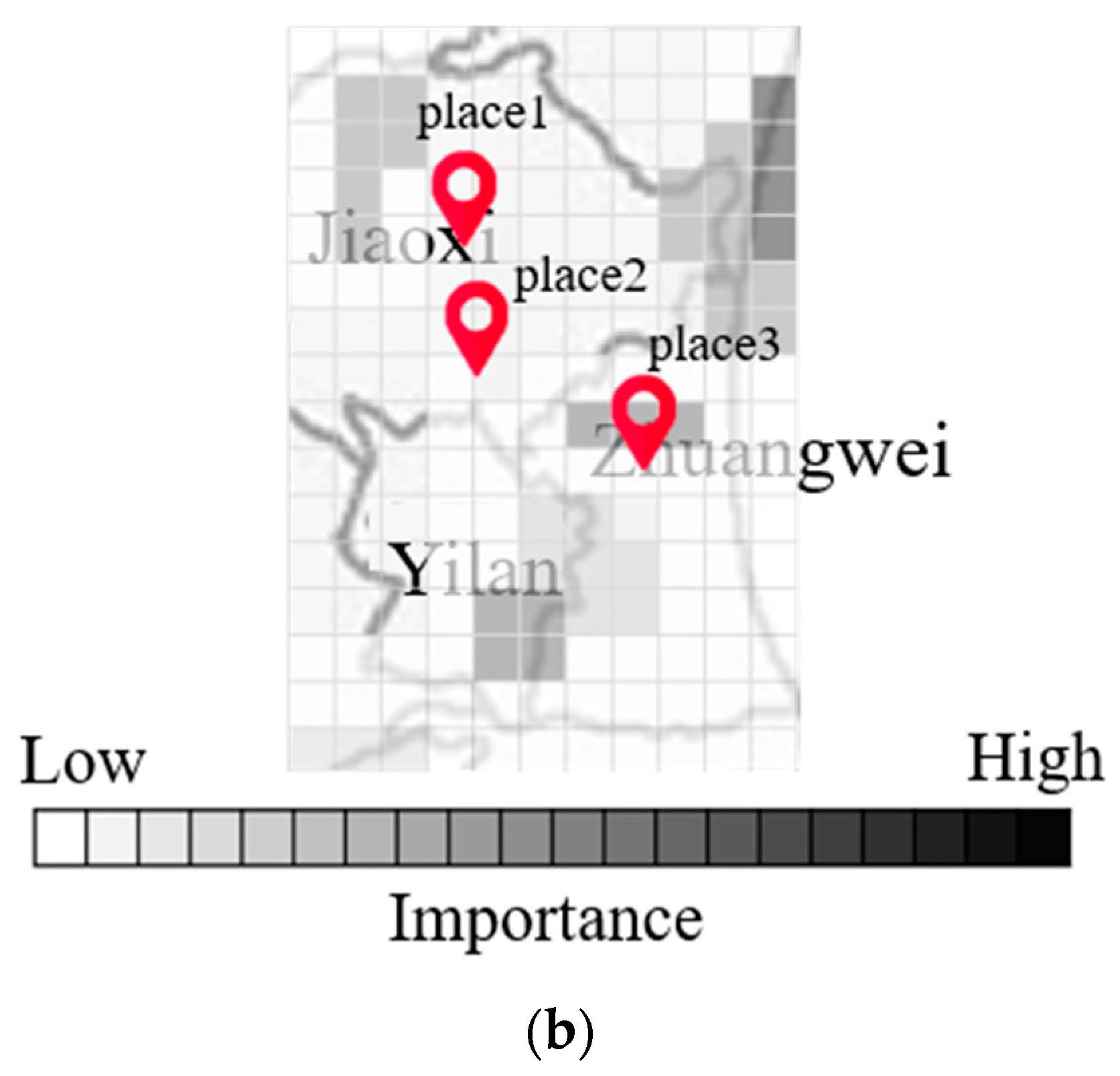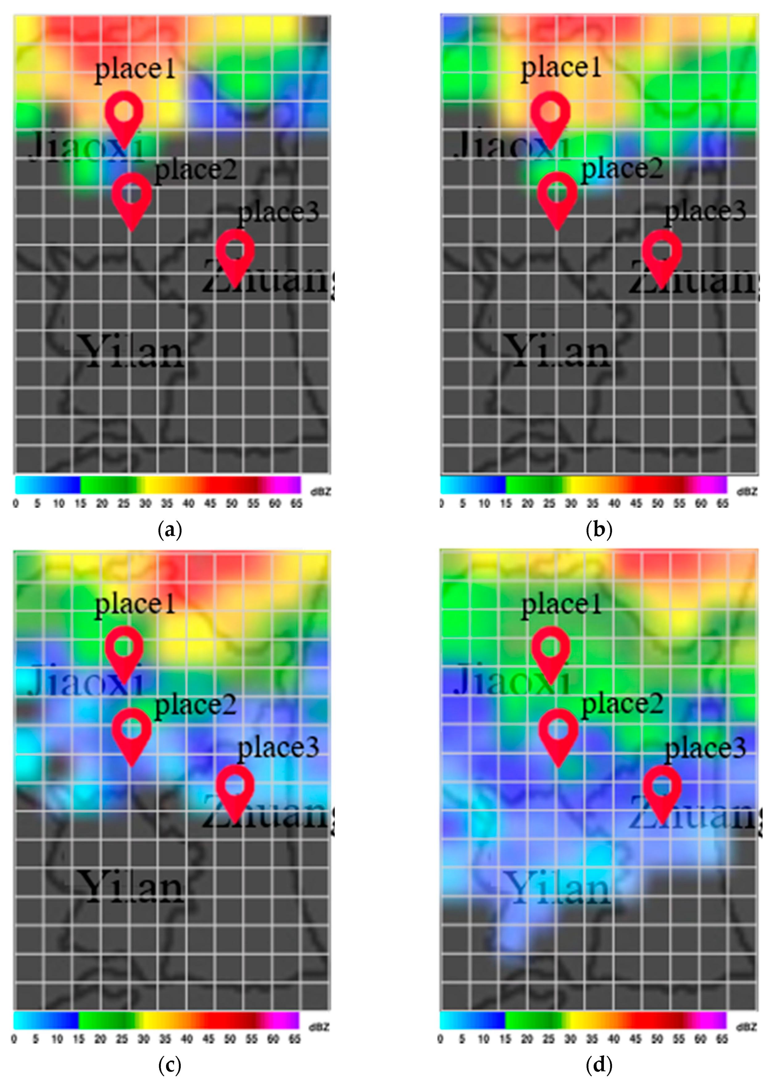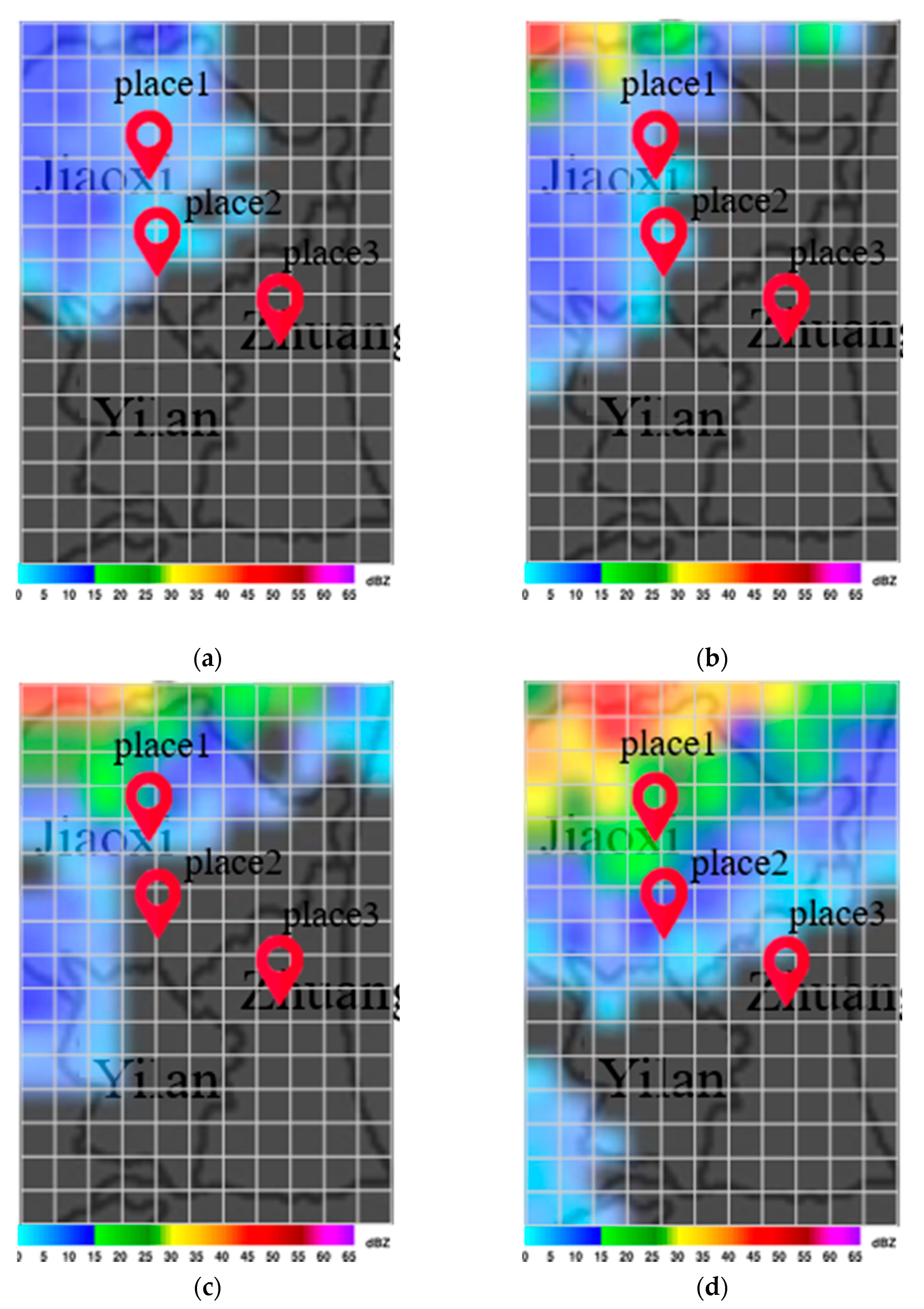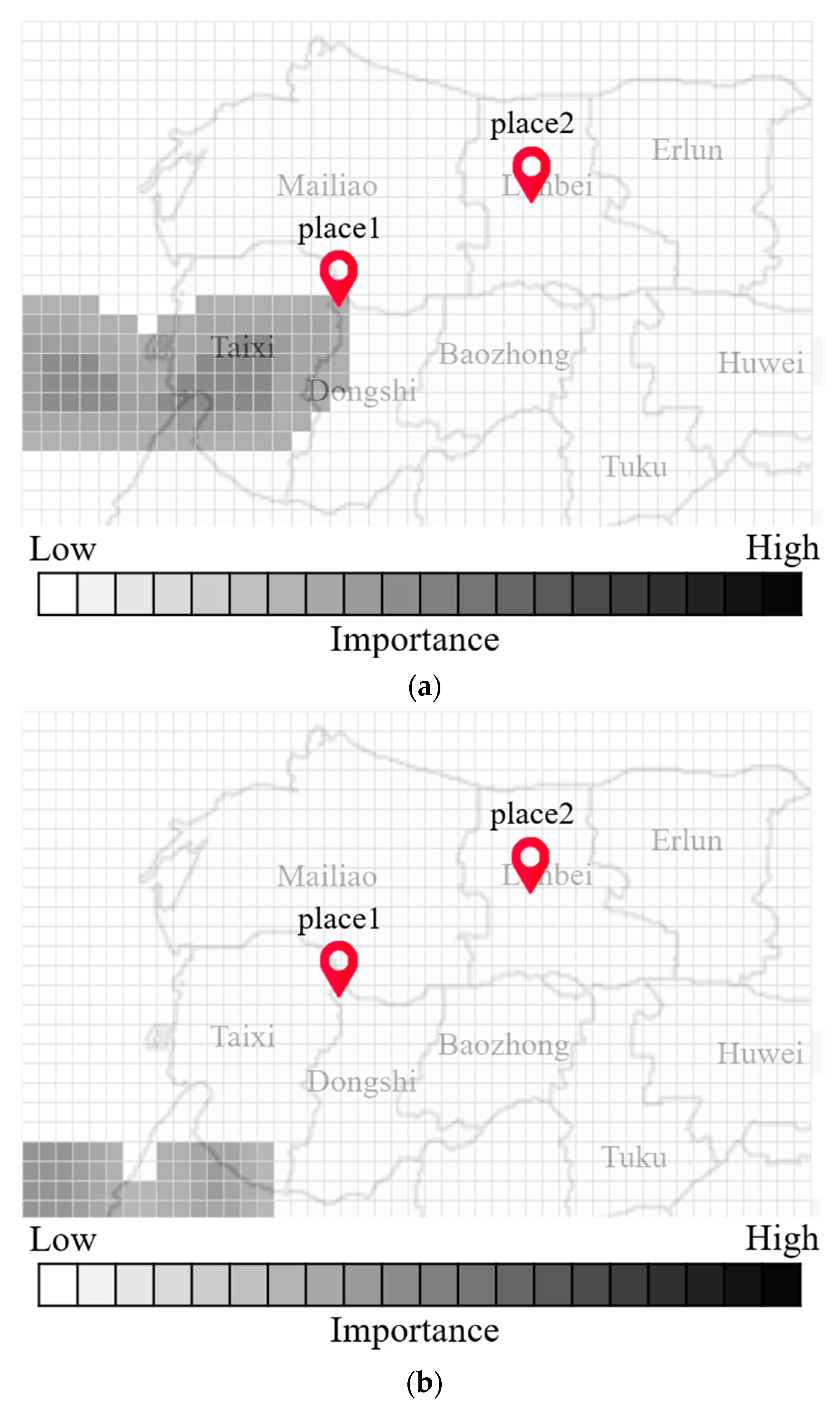Figure 7a,b present maps indicating the degree of importance after inputting multiple radar echo maps into the CNN to derive the flood height. Note that the degree of blackening is proportional to the influence on the output value. Note also that the maps generated by Grad-Cam differ according to input, as shown in Figure 7a,b. Differences in input data can have a profound influence on the output of each grid cell.

The formula used to calculate Grad-Cam is derived under the assumption that the length and width of the feature map set are m_f and n_f, the channel size is s_c, and the output result of the CNN is ô. We can calculate the weight w_c of the cth channel of the feature map f_c as follows:

$$w_c=\frac{1}{m_f\times n_f}{\displaystyle \sum _{m_f}{\displaystyle \sum _{n_f} }}\frac{\partial \widehat{o}}{\partial f_c},$$

(9)

where 1/(m_f × n_f) is the term used to calculate global average pooling, and ∂ô/∂f_c are gradients obtained via back propagation. We then combine the degree of importance of all feature maps to derive the degree to which each input grid cell influences the CNN output:

$$\mathrm{W}=Relu({\displaystyle \sum _c^{s_c}{w}_c f_c}).$$

(10)

Note that the above formula also uses the Relu function to set all negative numbers to 0, and thereby complete the calculations.

Grad-Cam calculates the degree to which individual grid cells influence the output value corresponding to each input datum and generates a matrix representing the degree of influence. Thus, if we input n pieces of data into the CNN, then we should obtain n matrices; however (as mentioned previously), the grid cells representing a given location in different matrices may have different values. This makes it difficult to identify the key grid cells for modeling. Thus, we use following formula to calculate the importance of each grid cell.

$$Fimp\left(i, j\right)=\raisebox{1ex}{$1$}\!\left/ \!\raisebox{-1ex}{$n$}\right.{\displaystyle {\sum }_{k=1}^{n}imp\left(i, j\right)}\times w_k,$$

(11)

where n is the total number of input data, imp_k(i,j) indicates the importance of grid cell (i,j) calculated by Grad-Cam for the kth input data (1 ≤ k ≤ n), Fimp(i,j) is the final importance calculation for grid cell (i,j), w_k is the weight value given by the user, indicating the degree of importance assigned by the user to each input. If the user believes that each piece of input data is of equal importance in prediction, then w_k is set to 1. Finally, Equation (11) can be used to rank the importance of all grid cells from large to small, whereupon the top-ranking cells are selected as key grid cells.

3.4. Lightweight Deep Neural Networks (LDNNs)

The key grid cells are treated as independent dimensions to be input into an LDNN for modeling. From a theoretical perspective, most of the regression models used in conventional machine learning, such as support vector regression [32,33], k-nearest neighbors [34,35], and Random Forest [36,37,38], could be used as an alternative to LDNN; however, we elected to use a deep neural network (DNN) in order to maximize prediction accuracy. Note that the number of key grid cells is far smaller than the number of cells in the entire radar echo map. Under these conditions, the computational cost of an LDNN is far lower than that of the CNN in the previous section.

The structure of the LDNN used in this paper is introduced in the following section, as shown in Figure 8. The total number of layers and the number of neurons in each layer varied as a function of input (key grid cells). Note that the input layer is responsible only for transmitting input data. In the network, the number of neurons is equal to the number of key grid cells extracted in the previous step. The first fully connected layer is used to increase dimensionality. Assuming that the input layer has a total of n neurons, there will be 2^ceiling(log₂n) neurons in this layer, where ceiling(•) represents the unconditional roundup function. The number of neurons after the second fully connected layer decreases by a multiple of 2 or 4 until reaching 1, and the last layer is the output layer. Without a loss of generality, the formula in each neuron of fully connected layers can be written as follows:

$$o_j=\tanh (t_j\times w_{ij})+b_j.$$

(12)

where o_j represent the output of a given node, tanh(•) is the tangent sigmoid function, w_ij is the corresponding weight, and b_i is the bias vector corresponding to the jth neuron.

Generally, the implementation of a neural network can be divided into offline model establishment procedures (training, testing, and verification) and online operational procedures. The time required to establish the model is dominated by the dimensionality of data input m and the number of data items in the dataset n. Note that m affects the calculation time after data is input into the model. Increasing m produces a corresponding increase in the numbers of layers, neurons, and weights between neurons, which increases the computational overhead. Note that n mainly affects the model training time. By reducing the value of m, an LDNN can reduce the time required to complete offline establishment procedures. Online calculation time generally refers to the time required to process an input after the model has been implemented online. This value depends largely on system capacity and the number of input dimensions m. In other words, LDNN reduces online calculation time by reducing the value of m.

4. Simulation Experiments

Real-world radar echo maps and data sets gathered from flood sensors were used to verify the effectiveness of our proposed method. In the following, we outline the data sets and experiment parameters as well as the parameter indicating the time delay between the radar echo map input and flood height output. We then examine the effectiveness of the LDNN and explain our reasons for selecting particular feature values.

4.1. Data Sets and Experiment Parameters

The regions of interest in this experiment were two counties in Taiwan (Yilan and Yunlin). These areas were selected because Taiwan is among the most flood-prone places in the world and these counties are the most flood-prone in Taiwan. Figure 9 illustrates the locations of these counties within Taiwan and the corresponding topography. As shown in Figure 9a, Yilan is located in the northeastern region of Taiwan, whereas Yunlin is located in the western region, with 3000 m mountains between them. The weather systems in the two locations are entirely disconnected; therefore, we are confident that the causes of flooding in the two places are quite different. Yilan is surrounded by mountains on three sides and the sea to the east, as shown in Figure 9b. Its location on the windward side of the monsoon during the summer produces rain on more than half of the days each year. In times of heavy rain, the surrounding plains can also be affected by surging mountain rivers flowing to the sea. Frequent flooding occurs in areas with inadequate drainage. The landscape of Yunlin consists mostly of plains. As shown in Figure 9c, it is bordered by hills to the east and directly faces the sea to the west. Most of the rainfall is caused by air currents from the southwest. The average rainfall is similar to that in other regions of Taiwan; however, the over-pumping of groundwater for agriculture has resulted in severe stratum subsidence, which increases the risk of flooding under the effects of heavy rain.

Our flood data were based on the well-known Taiwanese open-source platform Civil IoT Taiwan, Data Service Platform [39]. This platform (established by the government) uses a range of sensor data, including water level, river flow, catchment slope change, reservoir water level, water quality, soil water content, and irrigation canal flow. In the current study, we focused on flood height readings from water level gauges installed at the bottom of poles along roads. Photographs of actual water level gauges are presented in Figure 10. Note also that we focused on flooding along public roads (i.e., disregarding river water levels), due to the fact that the conditions along these corridors are of particular importance in terms of public safety.

To limit the amount of data requiring processing, we selected the areas and months with the most frequent flooding in Yilan and Yunlin, based on data from all water level gauges in the regions of interest. This included three points in Yilan in June 2020 and two points in Yunlin area in May 2020 (see Figure 11). Note that none of these locations are located on the seaside or riverside, thereby ensuring that the flood height would not be affected by the tides or the height of the river. These locations conform to the research limitations of this paper, which focuses exclusive on the use of radar echo maps as inputs for prediction. We also listed a time series of flood heights (Figure 12), a box and whisker diagram of flood height (Figure 13), and statistics of flood height (

Table 1. Statistics of flood heights in five monitoring locations.

	Yilan			Yunlin
	Place 1	Place 2	Place 3	Place 1	Place 2
Average	0.645	0.598	0.363	1.332	0.595
Standard Deviation	4.565	1.187	1.896	1.083	0.997
Number of data in the dataset	4320	4320	4320	4464	4464
Number of flooded data in the dataset	526	658	834	1143	2761
Number of data used in the experiment	1052	1316	1668	2286	4464

). Note that the units used to denote water levels in these charts match those of the water level gauges (cm). Table 1 lists the volumes of data collected for each monitoring point and the amount of data cleaned during the time period of interest. Overall, 70% of the data was used for training, 10% was used for testing, and 20% was used for validation. In addition, since the experimental data in this paper are not sufficient to divide the training, validation, and test data sets into different flooding events, we only use the method of random selection to compose these three data sets.

Radar echo maps were based on data released by the Central Meteorological Bureau of Taiwan. The map can be divided into three channels: R, G, and B. Each cell in the original maps measured 350 × 350 m; however, the use of high-resolution maps to represent the large area of Yilan (13 × 20 km) and Yunlin (53 × 31 km) would exceed the computational capacity of the experiment environment. We thus decreased the map resolution by increasing the size of grid cells to 1050 × 1050 m. The resulting radar echo map of the Yilan area included 11 × 16 cells (Figure 14a), whereas the map of the Yunlin area included 47 × 28 cells (see Figure 14b).

In this paper, we did not specifically adjust the parameters of the CNN. Rather, we used presets in the Python Tensorflow suite. For example, the batch size for model training was set at 20, the number of epochs was set at 100, the loss function was “mse”, and the metrics was “mae”. Our primary focus in this study was to verify the feasibility of using CNN and Grad-Cam for lightweight models. We opted to use the default values to avoid affecting the verification results. Next, as a proxy for wind speed and cloud movement, we examined the degree to which radar echo maps influenced flood height in the target location at intervals of 30 min (30 min, 60 min, 90 min, 120 min, and 150 min). We employed the well-known early stopping procedure, which has proven highly effective in preventing the problem of overfitting during model training in a range of applications [40,41,42]. The judgment benchmark was 20 epochs, and the Adam optimizer was used with an initial learning rate of 0.001. All experimental simulations in this study were implemented in Python under the Windows 10 64-bit operating system using an Intel 2-core Xeon Processor (2.20 GHz) with 32 GB of memory.

4.2. Selection of CNN Time Delay Parameter Indicating the Difference between the Radar Echo Map Input and Flood Height Output

In this section, we describe the experiments used to guide the selection of the time delay parameter.

Table 2. Impact of time delay on the prediction results in various monitoring locations.

Time Delay	Yilan			Yunlin
	Place 1	Place 2	Place 3	Place 1	Place 2
30 min	4.309	0.192	2.203	1.775	0.706
60 min	4.514	1.873	2.348	2.688	1.641
90 min	5.023	1.932	2.614	2.83	1.549
120 min	5.314	2.306	3.431	3.691	1.978
150 min	5.967	2.684	3.739	5.034	2.261

lists the results with the time delay set to 30 min, 60 min, 90 min, 120 min, or 150 min. Note that the error in Table 2 is described using root-mean-square error (RMSE) between the flood height predicted by the model and the actual flood height. This evaluation was used to make it easier for readers to compare model errors with actual data. In all locations, prediction accuracy decreased with an increase in delay time. This is a reasonable result, considering the rapid changes in radar echo maps, which essentially preclude the use for earlier maps to make predictions pertaining to the current map or current flood height. We determined that using the radar echo map of the first 30 min yielded better flood prediction results; therefore, we used this time delay for all subsequent experiments as the input for the CNN and LDNN.

4.3. Effectiveness of LDNN

In this section, we discuss the prediction performance and computational overhead of the proposed LDNN. We divided the content into three parts: (1) selection of key grid cells at each monitoring site, (2) comparison of original CNN model and LDNN model in terms of prediction error, and (3) comparison of original CNN model and LDNN model in terms of computational overhead.

Table 3. Impact of the number of key grid cells on prediction results in various locations.

Number of Key Grid Cells	Yilan			Yunlin
	Place 1	Place 2	Place 3	Place 1	Place 2
10	4.286	0.401	2.203	1.23	0.947
20	4.351	0.359	2.231	1.175	1.252
30	4.215	0.293	2.468	1.16	1.303
40	3.948	0.285	2.649	1.169	1.342
50	3.907	0.296	2.591	1.194	1.353
60	3.97	0.281	2.672	1.189	1.369
70	4.621	0.21	2.73	1.206	1.368
80	5.296	0.192	2.794	1.214	1.376
90	5.684	0.275	2.943	1.218	1.393
100	6.102	0.33	2.926	1.23	1.405

lists the key grid cells selected for each monitoring station. The horizontal axis of the table indicates the monitoring location, and the vertical axis lists the prediction result as a function of the number of key grid cells input into the LDNN. Note that error in Table 3 is represented in terms of RMSE. The bold numbers indicate the optimal number of key grid cells for a given observation site. From a theoretical perspective, the number of key grid cells should be increased in intervals of 1 in order to obtain the optimal solution. From a practical perspective, however, we had to deal with a large number of grid cells (176 in Yilan and 1316 in Yunlin), which essentially precluded small incremental increases. We thus began with 10 key grid cells and increased this in increments of 10 until 100 cells were selected. The data in Table 3 revealed two important findings. First, LDNN predicted that RMSE would first decrease with an increase in the number of key grid cells and then increase after reaching the highest prediction accuracy, regardless of observation location. A small number of key grid cells would not provide sufficient information to build a model for the prediction of flood height, resulting in large prediction error. Increasing the number of grid cells would provide more information with which to build models to predict flood height, thereby reducing prediction error. Increasing the number of grid cells beyond the optimal value would result in excessive information leading to conflicts among the results for various cells, with a corresponding increase in prediction error. Second, the optimal number of key grid cells varied with the monitoring location. For example, the optimal number of key grid cells for the three locations in Yilan were 50, 80, and 10. The optimal number of key grid cells in Yunlin were 10 and 30. From this, we postulate that in cases where the relationship between the cause(s) of flooding and radar echo maps is simple, it should be possible to obtain good prediction results using a small number of key grid cells, and vice versa. This issue is detailed in the next section. For the sake of convenience, the number of key grid cells in all subsequent experiments are the optimal solutions listed in Table 3.

Table 4. Comparison of original CNN and the LDNN in terms of prediction error.

Model	Yilan			Yunlin
	Location 1	Location 2	Location 3	Location 1	Location 2
CNN	4.309	0.192	2.203	1.775	0.706
LDNN (all)	4.738	0.3	2.702	1.945	1.336
LDNN (n)	3.907	0.192	2.203	1.16	0.947

compares the original CNN and the LDNN in terms of prediction errors, based on three sets of experiments: prediction error of original CNN (indicated by CNN), error after inputting all grid cells into the LDNN as independent dimensions (indicated by LDNN(all)), and error of inputting only key grid cells into the LDNN (indicated by LDNN(n)). Note that error in Table 4 is represented using RMSE. In this table, we first discuss why the RMSE of different place are quite different. This is because in most neural network models, prediction error is affected by the magnitude of variations in the original data. The model used in the current paper was based on a neural network; therefore, our situation was similar. There were large differences in flood height between the five observation sites, with the result that our prediction errors differed significantly from one location to another. Table 1 indicates the standard deviation and prediction errors associated with CNN, LDNN(all), LDNN(n) for flood records in the five locations selected for this paper. Figure 13 presents a box map of the flooding records at the five sites. From Table 1, we can see that the standard deviation at the five locations varied as follows: Yilan location 1 > Yilan location 3 > Yilan location 2 ≈ Yunlin location 1 ≈ Yunlin location 2. As a result, the prediction errors for Yilan location 1 and Yilan location 3 were far more pronounced than for the other three locations. Moreover, we can see in Figure 13 that the data distribution range for the other three locations was as follows: Yunlin location 1 > Yunlin location 2 > Yilan location 2, and the model prediction error followed the same pattern.

In Table 4, we can see that regardless of the monitoring location, LDNN(all) was outperformed by the original CNN in terms of accurcy This can be explained by the fact that compared with the CNN, the LDNN architecture does not place as much emphasis on information from adjacent cells. Thus, even in cases where all of the values were the same, the prediction performance of LDNN was worse. Based on this insight, we can conclude that in subsequent experiments, as long as the performance of LDNN(n) does not deviate far from that of the CNN, differences in accuracy cannot be attributed to differences in architecture, but rather to the selection of a reasonable key grid cell. In the two subsequent experiments, the prediction performance of LDNN(n) was roughly on par with that of the CNN, regardless of location. This can be explained by the fact that the CNN and LDNN(n) used the same grid information, despite the fact that the CNN used key grid cells selected via adaptive learning, whereas LDNN(n) used key grid cells selected by Grad-Cam. In other words, the grids used in the models were the same; therefore, modeling accuracy was also nearly the same. Note, however, that the LDNN also possesses some characteristics of adaptive learning, such that in a few cases, it was able to extract more critical information and thereby achieve prediction results of higher accuracy (see location 1 in Yilan and location 1 in Yunlin). Overall, the proposed LDNN(n) achieved prediction performance on par with that of the CNN; however, the prediction performance of the LDNN was slightly worse than that of the CNN in one monitoring location (see locations 2 in Yunlin). This can be explained by the fact that Grad-Cam made an error in key grid cell extraction. This issue is discussed in greater detail in the next section.

Table 5. Comparison of original CNN and LDNN in terms of training cost.

Type of Costs	Yilan			Yunlin
	Location 1	Location 2	Location 3	Location 1	Location 2
Time-CNN	1920 s	1884 s	1936 s	2316 s	2340 s
Time-LDNN	105 s	173 s	68 s	142 s	120 s
Time-Reduced ratio	94.5%	90.8%	96.4%	93.9%	94.9%
Memory-CNN	814 MB	821 MB	817 MB	930 MB	926 MB
Memory-LDNN	64 MB	92 MB	50 MB	92 MB	79 MB
Memory-Reduced ratio	92.1%	88.8%	93.9%	90.1%	91.5%

and

Table 6. Comparison of original CNN and LDNN in terms of online operating cost.

Type of Costs	Yilan			Yunlin
	Location 1	Location 2	Location 3	Location 1	Location 2
Time-CNN	58 s	56 s	58 s	94 s	96 s
Time-LDNN	9 s	11 s	6 s	10 s	8 s
Time-Reduced ratio	84.5%	80.3%	89.6%	89.4%	91.7%
Memory-CNN	68 MB	71 MB	70 MB	97 MB	94 MB
Memory-LDNN	20 MB	24 MB	15 MB	33 MB	30 MB
Memory-Reduced ratio	70.5%	66.2%	78.5%	66.0%	68.1%

illustrate the computational costs of the CNN and LDNN models. The training time of the LDNN was roughly 95% lower than that of the CNN after key grid cells were identified, and memory usage was roughly 90% lower. Training costs this low would no doubt be of considerable benefit in training multiple models for large geographic regions. This configuration would also facilitate the retraining of models, thereby shortening the update cycle to improve the accuracy of predictions. As shown in Table 6, we simulated the costs involved in predicting the flood height using multiple grids covering a large area. The simulation involved running the models 100 times, as would be the case when predicting 100 target places. As shown in the table, time cost of training the LDNN was 85% lower than that of the CNN and the memory cost was roughly 70% lower. Under these conditions, the LDNN would be able to update the values of roughly 5500 target places every 10 min, whereas the CNN would be limited to updating 650–1000 target places. The heavy memory requirements of the CNN would also necessitate the purchase of larger computer systems.

4.4. Key Grid Cell Selection: Rationale

From a qualitative perspective, we sought to determine whether the key grid cells indeed influenced flood height predictions at the target observation site. The two target areas of Yilan and Yunlin are discussed separately.

Figure 15 present the key grid cells selected from the Grad-Cam results of the three observation sites in Yilan. We can see that regardless of the observation site, all key grid cell–cell combinations included grids over the sea northeast of Yilan. This appears reasonable, based on the fact that most of the rainfall in Yilan is carried in by rain clouds from the northeast to strike the mountains to the west of Yilan (see Section 4.1). Most of these rain clouds were located over the sea to the northeast of Yilan at 30 min prior to the onset of flooding (the time difference between the input radar echo map and the output), as evidenced by the radar echo maps of the flood events in Figure 16 and Figure 17. We also examined key grid cells other than those in the northeast (see Figure 15). Due to the location of Observation Station 1 to the north of the city, the key grid cells differ from those associated with the other Yilan stations, as shown in Figure 15a. Observation Station 2 is located near the Dongshan River (largest river in Yilan), such that flooding in that area is affected by the river level as well as rainfall. Thus, it is not surprising to observe that the key grid cells were located in upstream areas of the Dongshan River and its tributaries, as shown in Figure 15b. Observation Station 3 it is located by the sea and there is no large water system around it; therefore, rainfall in other places in Yilan did not affect flood height in the vicinity of this station, with the result that no additional key grid cells were identified, as shown in Figure 15c.

Figure 18a,b present the corresponding key grid cells selected by Grad-Cam for the monitoring stations in Yunlin. Most of the rainfall in Yunlin during May and June is caused by airflow from the southwest (see Section 4.1). Thus, flooding at Observation Station 1 should theoretically be correlated with flooding in the southwest roughly 30 min before. The key grid cell selection results in Figure 18a confirm a strong correlation between rain clouds and key grid cells located to the southwest. As mentioned in the previous section, the LDNN prediction results for Observation Station 2 were inferior to the CNN results. Figure 18b shows that the key grid cells are located to the southwest of Observation Station 2; however, the distance between Observation Station 2 and its key grid cells is greater than the distance between Observation Station 1 and its key grid cells. In this situation, LDNN was able to approximate the trends pertaining to flood height; however, the lower accuracy of the input information resulted in prediction error. In this situation, errors in key grid cell selection can partly be attributed to sensor settings at Observation Station 2. As shown in Figure 19, the sensor was placed on a slope next to a ditch, such that every time it rained (even without flooding), water flowing into the ditch passed the sensor, thereby erroneously indicating flood conditions. This kind of inaccuracy in the trained model no doubt affected Grad-Cam performance in the identification of key grid cells. Essentially, the radar echo map indicates the position of rain clouds at Observation Station 2, regardless of whether they are likely to produce heavy rainfall, with the result that the key grid cells are further south than those of Observation Station 1.

5. Conclusions

Climate change has exacerbated the problem of flooding around the globe. Research into the prediction of flood height during heavy rainfall has focused on the use of hydrological models in conjunction with radar echo maps. However, the construction of hydrological models requires highly specialized professional knowledge and extensive measurement data. Furthermore, many hydrological models fail to consider all relevant factors specific to the target site, thereby compromising the accuracy of predictions. This is the first study to use a DLM for the prediction of flood height directly from radar echo maps. We overcame the heavy computational burden of DLMs by implementing a novel LDNN, in which a CNN is trained using a radar echo map in conjunction with historical flood record at target sites. We then use the Grad-Cam package to extract key grid cells from the radar echo map (i.e., cells with the greatest impact on flood height prediction) as inputs into the LDNN for modeling and prediction. The efficacy of the proposed scheme was verified using simulations based on actual radar echo maps and records of flooding at sites in two discrete areas.

Note that this paper discusses only the modeling of relationship between radar echo maps and flood height, despite the fact that flooding is affected by factors other than rainfall (e.g., water levels in surrounding rivers or tides). Unfortunately, the data format used to quantify those factors is a single value, such that it cannot be presented in the grid format required for the proposed scheme. Thus, we will examine other (i.e., non-CNN) models and other data formats for use in lightweight DLM modeling. Note also that in places in which flood depth changes drastically, predicting flood depth using a single model can be difficult [43]. Thus, we are developing additional methods by which to overcome this issue. In addition to model improvements mentioned above, we consider whether the interaction of different flood factors, such as multiple elevations’ radar echo maps, terrain, land use, etc., may affect the accuracy of Grad-Cam’s judgment of key grid cells. We will study this in the future.

References

1. Mecklenburg, S.; Bell, V.A.; Moore, R.J.; Joss, J. Interfacing an enhanced radar echo tracking algorithm with a rainfall-runoff model for real-time flood forecasting. Phys. Chem. Earth Part B Hydrol. Ocean. Atmos. 2000, 25, 1329–1333. [Google Scholar] [CrossRef]
2. Šálek, M.; Brezková, L.; Novák, P. The use of radar in hydrological modeling in the Czech Republic—Case studies of flash floods. Nat. Hazards Earth Syst. Sci. 2006, 6, 229–236. [Google Scholar] [CrossRef]
3. Novák, P.; Březková, L.; Frolík, P. Quantitative precipitation forecast using radar echo extrapolation. Atmos. Res. 2009, 93, 328–334. [Google Scholar] [CrossRef]
4. Yoon, S.S. Adaptive blending method of radar-based and numerical weather prediction QPFs for urban flood forecasting. Remote Sens. 2019, 11, 642. [Google Scholar] [CrossRef] [Green Version]
5. Chen, L.; Cao, Y.; Ma, L.; Zhang, J. A Deep Learning-Based Methodology for Precipitation Nowcasting with Radar. Earth Space Sci. 2020, 7, e2019EA000812. [Google Scholar] [CrossRef] [Green Version]
6. Yin, X.; Hu, Z.; Zheng, J.; Li, B.; Zuo, Y. Study on Radar Echo-Filling in an Occlusion Area by a Deep Learning Algorithm. Remote Sens. 2021, 13, 1779. [Google Scholar] [CrossRef]
7. Singh, S.; Sarkar, S.; Mitra, P. A deep learning based approach with adversarial regularization for Doppler weather radar ECHO prediction. In Proceedings of the 37th IEEE International Geoscience and Remote Sensing Symposium (IGARSS 2017), Fort Worth, TX, USA, 23–28 July 2017; pp. 5205–5208. [Google Scholar]
8. Yin, J.; Gao, Z.; Han, W. Application of a Radar Echo Extrapolation-Based Deep Learning Method in Strong Convection Nowcasting. Earth Space Sci. 2021, 8, e2020EA001621. [Google Scholar] [CrossRef]
9. Yan, Q.; Ji, F.; Miao, K.; Wu, Q.; Xia, Y.; Li, T. Convolutional residual-attention: A deep learning approach for precipitation nowcasting. Adv. Meteorol. 2020, 2020. Available online: https://www.hindawi.com/journals/amete/2020/6484812/ (accessed on 2 December 2021). [CrossRef]
10. Han, S.; Mao, H.; Dally, W.J. Deep compression: Compressing deep neural networks with pruning, trained quantization and huffman coding. In Proceedings of the 4th International Conference on Learning Representations (ICLR 2016), San Juan, Puerto Rico, 2–4 May 2016; pp. 1–14. [Google Scholar]
11. Li, H.; Kadav, A.; Durdanovic, I.; Samet, H.; Graf, H.P. Pruning filters for efficient ConvNets. In Proceedings of the 5th International Conference on Learning Representations (ICLR 2017), Toulon, France, 24–26 April 2017; pp. 1–13. [Google Scholar]
12. Molchanov, P.; Mallya, A.; Tyree, S.; Frosio, I.; Kautz, J. Importance estimation for neural network pruning. In Proceedings of the 32th IEEE/CVF Conference on Computer Vision and Pattern Recognition (CVPR 2019), Long Beach, CA, USA, 15–20 June 2019; pp. 11264–11272. [Google Scholar]
13. Luo, J.H.; Wu, J.; Lin, W. Thinet: A filter level pruning method for deep neural network compression. In Proceedings of the 16th IEEE International Conference on Computer Vision (ICCV 2017), Venice, Italy, 22–26 October 2017; pp. 5058–5066. [Google Scholar]
14. Sani, S.; Wiratunga, N.; Massie, S. Learning deep features for knn based human activity recognition. In Proceedings of the 25th International Conference on Case-Based Reasoning Workshops (ICCBR 2017), Trondheim, Norway, 26–28 June 2017; pp. 95–103. [Google Scholar]
15. Mohammad, Y.; Matsumoto, K.; Hoashi, K. Deep feature learning and selection for activity recognition. In Proceedings of the 33rd Annual ACM Symposium on Applied Computing (SAC 2018), Pau, France, 9–13 April 2018; pp. 930–939. [Google Scholar]
16. Chen, Y.C.; Li, D.C. Selection of key features for PM2.5 prediction using a wavelet model and RBF-LSTM. Appl. Intell. 2021, 51, 2534–2555. [Google Scholar] [CrossRef]
17. He, T.; Guo, J.; Chen, N.; Xu, X.; Wang, Z.; Fu, K.; Yi, Z. MediMLP: Using grad-CAM to extract crucial variables for lung cancer postoperative complication prediction. IEEE J. Biomed. Health Inform. 2019, 24, 1762–1771. [Google Scholar] [CrossRef]
18. Li, Y.; Yang, H.; Li, J.; Chen, D.; Du, M. EEG-based intention recognition with deep recurrent-convolution neural network: Performance and channel selection by Grad-CAM. Neurocomputing 2020, 415, 225–233. [Google Scholar] [CrossRef]
19. Marsot, M.; Mei, J.; Shan, X.; Ye, L.; Feng, P.; Yan, X.; Zhao, Y. An adaptive pig face recognition approach using Convolutional Neural Networks. Comput. Electron. Agric. 2020, 173, 105386. [Google Scholar] [CrossRef]
20. Thorndahl, S.; Nielsen, J.E.; Jensen, D.G. Urban pluvial flood prediction: A case study evaluating radar rainfall nowcasts and numerical weather prediction models as model inputs. Water Sci. Technol. 2016, 74, 2599–2610. [Google Scholar] [CrossRef]
21. Wang, X.; Kinsland, G.; Poudel, D.; Fenech, A. Urban flood prediction under heavy precipitation. J. Hydrol. 2019, 577, 123984. [Google Scholar] [CrossRef]
22. Jati, M.I.H.; Santoso, P.B. Prediction of flood areas using the logistic regression method (case study of the provinces Banten, DKI Jakarta, and West Java). J. Phys. Conf. Ser. 2019, 1367, 012087. [Google Scholar] [CrossRef]
23. Berkhahn, S.; Fuchs, L.; Neuweiler, I. An ensemble neural network model for real-time prediction of urban floods. J. Hydrol. 2019, 575, 743–754. [Google Scholar] [CrossRef]
24. Arora, A.; Arabameri, A.; Pandey, M.; Siddiqui, M.A.; Shukla, U.K.; Bui, D.T.; Bhardwaj, A. Optimization of state-of-the-art fuzzy-metaheuristic ANFIS-based machine learning models for flood susceptibility prediction mapping in the Middle Ganga Plain, India. Sci. Total Environ. 2021, 750, 141565. [Google Scholar] [CrossRef]
25. Kabir, S.; Patidar, S.; Xia, X.; Liang, Q.; Neal, J.; Pender, G. A deep convolutional neural network model for rapid prediction of fluvial flood inundation. J. Hydrol. 2020, 590, 125481. [Google Scholar] [CrossRef]
26. Hsu, S.Y.; Chen, T.B.; Du, W.C.; Wu, J.H.; Chen, S.C. Integrate weather radar and monitoring devices for urban flooding surveillance. Sensors 2019, 19, 825. [Google Scholar] [CrossRef] [Green Version]
27. Ichim, L.; Popescu, D. Flooded areas evaluation from aerial images based on convolutional neural network. In Proceedings of the 37th IEEE International Geoscience and Remote Sensing Symposium (IGARSS 2017), Fort Worth, TX, USA, 23–28 July 2017; pp. 9756–9759. [Google Scholar]
28. Hata, E.; Seo, C.; Nakayama, M.; Iwasaki, K.; Ohkawauchi, T.; Ohya, J. Classification of aortic stenosis using ECG by deep learning and its analysis using grad-CAM. In Proceedings of the 42nd Annual International Conference of the IEEE Engineering in Medicine & Biology Society (EMBC 2020), Montréal, QC, Canada, 20–24 July 2020; pp. 1548–1551. [Google Scholar]
29. Chueh, K.M.; Hsieh, Y.T.; Ma, I.H.; Chen, H.H.; Huang, S.L. Differentiation of gender from macular optical coherence tomography using deep learning. In Proceedings of the 25th Opto-Electronics and Communications Conference (OECC 2020), Taipei, Taiwan, 4–8 October 2020; pp. 1–3. [Google Scholar]
30. Panwar, H.; Gupta, P.K.; Siddiqui, M.K.; Morales-Menendez, R.; Bhardwaj, P.; Singh, V. A deep learning and grad-CAM based color visualization approach for fast detection of COVID-19 cases using chest X-ray and CT-Scan images. Chaos Solitons Fractals 2020, 140, 110190. [Google Scholar] [CrossRef]
31. Seerala, P.K.; Krishnan, S. Grad-CAM-based classification of chest X-Ray images of pneumonia patients. In Proceedings of the 6th International Symposium on Signal Processing and Intelligent Recognition Systems (SIRS 2020), Chennai, India, 14–17 October 2020; pp. 161–174. [Google Scholar]
32. Zhang, J.; Teng, Y.F.; Chen, W. Support vector regression with modified firefly algorithm for stock price forecasting. Appl. Intell. 2019, 49, 1658–1674. [Google Scholar] [CrossRef]
33. Smola, A.J.; Schölkopf, B. A tutorial on support vector regression. Stat. Comput. 2004, 14, 199–222. [Google Scholar] [CrossRef] [Green Version]
34. Xu, Y.; Wang, L. K-nearest neighbor-based weighted twin support vector regression. Appl. Intell. 2014, 41, 299–309. [Google Scholar] [CrossRef]
35. Ohmori, S. A Predictive Prescription Using Minimum Volume k-Nearest Neighbor Enclosing Ellipsoid and Robust Optimization. Mathematics 2021, 9, 119. [Google Scholar] [CrossRef]
36. Malazi, H.T.; Davari, M. Combining emerging patterns with random forest for complex activity recognition in smart homes. Appl. Intell. 2018, 48, 315–330. [Google Scholar] [CrossRef]
37. Kim, S.; Jeong, M.; Ko, B.C. Lightweight surrogate random forest support for model simplification and feature relevance. Appl. Intell. 2021, 1–11. [Google Scholar] [CrossRef]
38. Wang, M.; Yue, L.; Cui, X.; Chen, C.; Zhou, H.; Ma, Q.; Yu, B. Prediction of extracellular matrix proteins by fusing multiple feature information, elastic net, and random forest algorithm. Mathematics 2020, 8, 169. [Google Scholar] [CrossRef] [Green Version]
39. Civil IoT Taiwan-Establishing IoT-Based Intelligent Environment Monitoring System. Available online: https://ci.taiwan.gov.tw/dsp/en/index.aspx (accessed on 2 December 2021).
40. Li, M.; Soltanolkotabi, M.; Oymak, S. Gradient descent with early stopping is provably robust to label noise for overparameterized neural networks. In Proceedings of the International conference on artificial intelligence and statistics, online, 26–28 August 2020; pp. 4313–4324. [Google Scholar]
41. Hazra, A.; Choudhary, P.; Inunganbi, S.; Adhikari, M. Bangla-Meitei Mayek scripts handwritten character recognition using Convolutional Neural Network. Appl. Intell. 2021, 51, 2291–2311. [Google Scholar] [CrossRef]
42. Prechelt, L. Early Stopping—But When? In Neural Networks: Tricks of the Trade. Lecture Notes in Computer Science; Springer: Berlin/Heidelberg, Germany, 1998; Volume 1524, pp. 55–69. [Google Scholar]
43. Chen, Y.C.; Lei, T.C.; Yao, S.; Wang, H.P. PM2.5 Prediction Model Based on Combinational Hammerstein Recurrent Neural Networks. Mathematics 2020, 8, 2178. [Google Scholar] [CrossRef]
Figure 1. Concept underlying the use of radar echo maps to predict flood height.
Water 14 00155 g001
Figure 2. Construction of lightweight model proposed in this work.
Water 14 00155 g002
Figure 3. Construction process of the proposed lightweight deep neural network (LDNN).
Water 14 00155 g003
Figure 4. Example showing why the target grid cell should not be centered in every case.
Water 14 00155 g004
Figure 5. Example illustrating the outcomes of time differences (time points and intervals) between flood sensors and the radar echo map.
Water 14 00155 g005
Figure 6. The internal structure of the proposed CNN.
Water 14 00155 g006
Figure 7. Example Grad-Cam result. (a) Example 1. (b) Example 2.
Water 14 00155 g007aWater 14 00155 g007b
Figure 8. The internal structure of the proposed LDNN.
Water 14 00155 g008
Figure 9. Map of study regions: (a) Location of Yilan and Yunlin within Taiwan; (b) detailed map of Yilan; (c) detailed map of Yunlin.
Water 14 00155 g009
Figure 10. Flood height indicator along public road: (a) Photographs of installation. (b) Photograph of water level gauges.
Water 14 00155 g010
Figure 11. The observation points in Yilan and Yunlin. (a) Yilan. (b) Yunlin.
Water 14 00155 g011aWater 14 00155 g011b
Figure 12. The time series of flood heights in five monitoring locations. (a) Yilan place 1. (b) Yilan place 2. (c) Yilan place 3. (d) Yunlin place 1. (e) Yunlin place 2.
Water 14 00155 g012aWater 14 00155 g012b
Figure 13. Box and whisker diagram of flood heights in five monitoring locations.
Water 14 00155 g013
Figure 14. The range of the radar echo map that we considered in two area. (a) Yilan. (b) Yunlin.
Water 14 00155 g014
Figure 15. Key grid cells selected from among Grad-Cam results in Yilan area. (a) Key grid cells of place 1. (b) Key grid cells of place 2. (c) Key grid cells of place 3.
Water 14 00155 g015
Figure 16. Radar echo maps of the actual flood event 1 in Yilan (26 June 2020, A.M. 04:40~05:10): (a) 04:40. (b) 04:50. (c) 05:00. (d) 05:10.
Water 14 00155 g016
Figure 17. Radar echo maps of the actual flood event 2 in Yilan (30 June 2020, A.M. 07:50~08:20): (a) 07:50. (b) 08:00. (c) 08:10. (d) 08:20.
Water 14 00155 g017
Figure 18. Key grid cells selected from the Grad-Cam results in Yunlin area. (a) Key grid cells of place 1. (b) Key grid cells of place 2.
Water 14 00155 g018
Figure 19. Sensor placement at Observation Station 2 in the Yunlin area.
Water 14 00155 g019