Comprehensive Assessment of Flood Hazard, Vulnerability, and Flood Risk at the Household Level in a Municipality Area: A Case Study of Nan Province, Thailand

Abstract

Estimating flood hazard, vulnerability, and flood risk at the household level in the past did not fully consider all relevant parameters. The main objective of this study is to improve this drawback by developing a new comprehensive and systematic methodology considering all relevant parameters and their weighting factors. This new methodology is applied to a case study of flood inundation in a municipal area of Nan City in the Upper Nan River Basin in Thailand. Field and questionnaire surveys were carried out to collect pertinent data for input into the new methodology for estimating flood hazard, vulnerability, and risk. Designed floods for various return periods were predicted using flood simulation models for assessing flood risk. The flood risk maps constructed for the return periods of 10–500 years show a substantial increase in flood risk with the return periods. The results are consistent with past flood damages, which were significant near and along the riverbanks where ground elevation is low, population density is high, and the number of household properties are high. In conclusion, this new comprehensive methodology yielded realistic results and can be used further to assess the effectiveness of various proposed flood mitigation measures.

1. Introduction

Floods are the most frequent type of disasters. They can cause widespread devastation, loss of life, and damage to personal property and public infrastructure. Between 1998 and 2017, floods affected more than 2 billion people, or 29% of the world population [1]. Floods cause more than USD 40 billion in damage worldwide annually [2]. The number of deaths due to the fact of significant floods worldwide from 1906 to 2014 was reported by Ritchie and Roser [3] (updated in 2020) as shown in Figure 1. In 1931, deaths were as high as 3.7 million in China, while in 1974, there were 28,700 deaths in Bangladesh [4].

People who live in floodplains or lack information on flood warning and flood hazard awareness are the most vulnerable to floods. Floods are expected to increase in frequency and intensity due to the anticipated increase in extreme precipitation as a result of continued climate change [5].

Many people tend to live in floodplain areas to satisfy needs for water and transportation. However, living in floodplain areas increases the risk to their assets, household, and life security during flooding [6,7,8]. A flood hazard, vulnerability, and risk assessment is necessary to determine the probability that a flood of a particular intensity may occur over an extended period of time [9]. A risk assessment aims to estimate this flooding probability from over a period of years to decades to support flood mitigation planning and management activities [10].

Extreme flood events can be more harmful to people living in the floodplain areas [11]. Another important consequence of floods is damage to physical infrastructures such as bridges, main roads, public buildings, and service facilities [12,13,14]. This type of structural damage is often defined as the amount of money needed to repair or rebuild. On the other hand, damages to populations and their household properties are related to socioeconomic conditions [15,16]. From flood hazard and flood vulnerability, flood risk can be determined, and flood risk maps can be constructed for various return periods for flood mitigation planning and management. A flood risk map can be helpful for land-use planning and management, reducing flood damage and saving human lives, agricultural products, and private and public properties.

Previous studies [17,18,19,20,21,22,23] considered flood hazard as a function of flood depth only or flood depth and velocity. This study considered all parameters including flood depth, velocity, inundation duration, and their weights. For the total vulnerability at the household level, this study considered all parameters including the sensitivity of the population, adaptive capacity, exposure of household properties, and their weights. These parameters have not been fully considered in the past.

The main aim of this study was to develop a comprehensive and systematic methodology for determining flood risks considering all hazard and vulnerability parameters and their weights using flood simulation models, questionnaire surveys, and the analytic hierarchy approach (AHP) [24,25]. The computational framework is given in Section 3 on the research structure and methodology.

The comprehensive and systematic methodology developed in this study is the main contribution, as it will be an essential foundation for properly assessing flood hazard, vulnerability, and flood risk in the future.

Hence, the objectives of this study were as follows:

(a)

To simulate floods in the Upper Nan River and its floodplain in the municipal area of Nan Province;

(b)

To develop a comprehensive and systematic methodology to determine flood hazard, flood vulnerability, and flood risk in a municipal area at the household level;

(c)

To apply the developed methodology to assess flood hazard, flood vulnerability, and flood risk at the household level in the Nan Municipality area considering floods of various return periods;

(d)

To analyze and discuss the consequences of flood hazard, vulnerability, and flood risk on local residents and the physical environment.

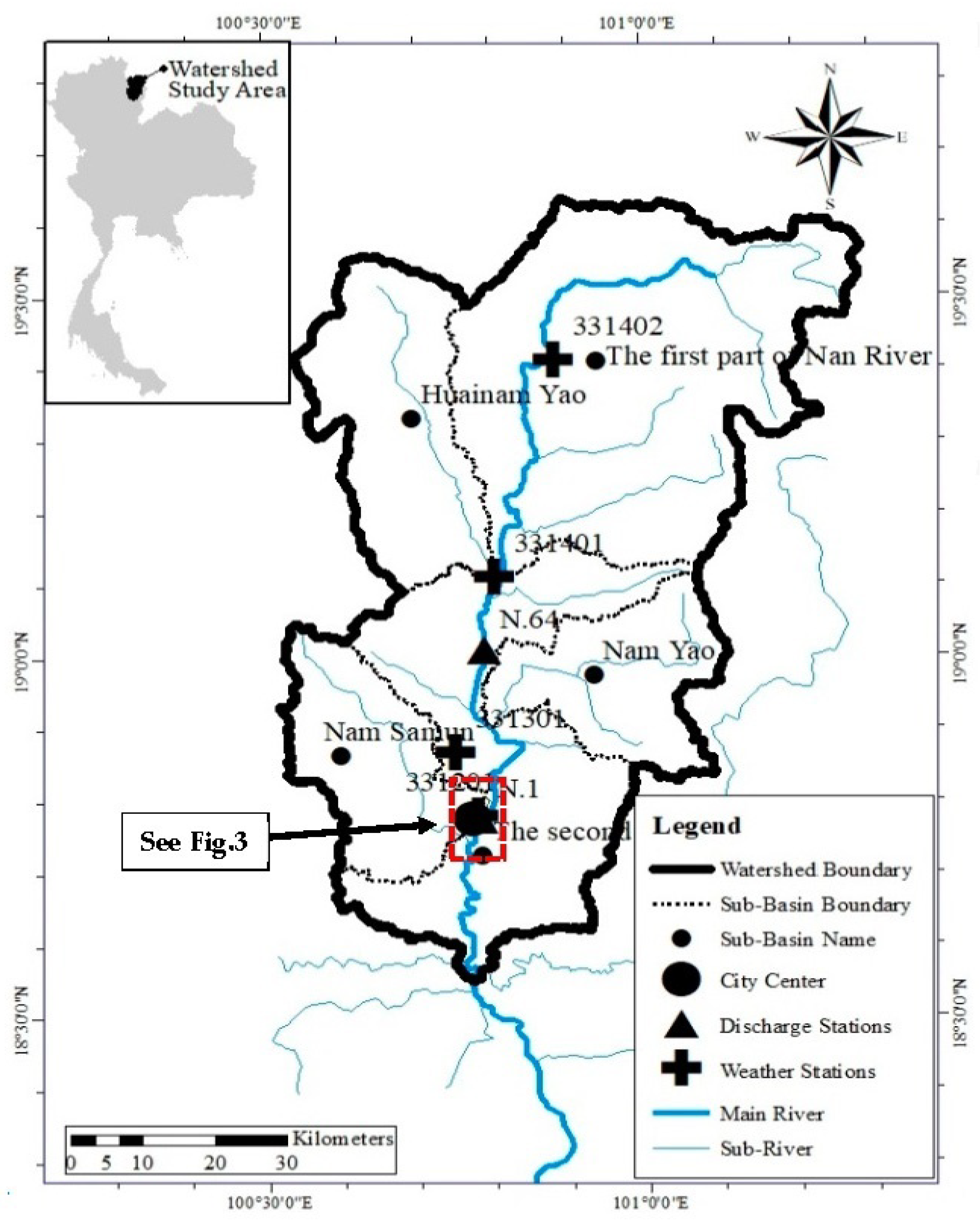
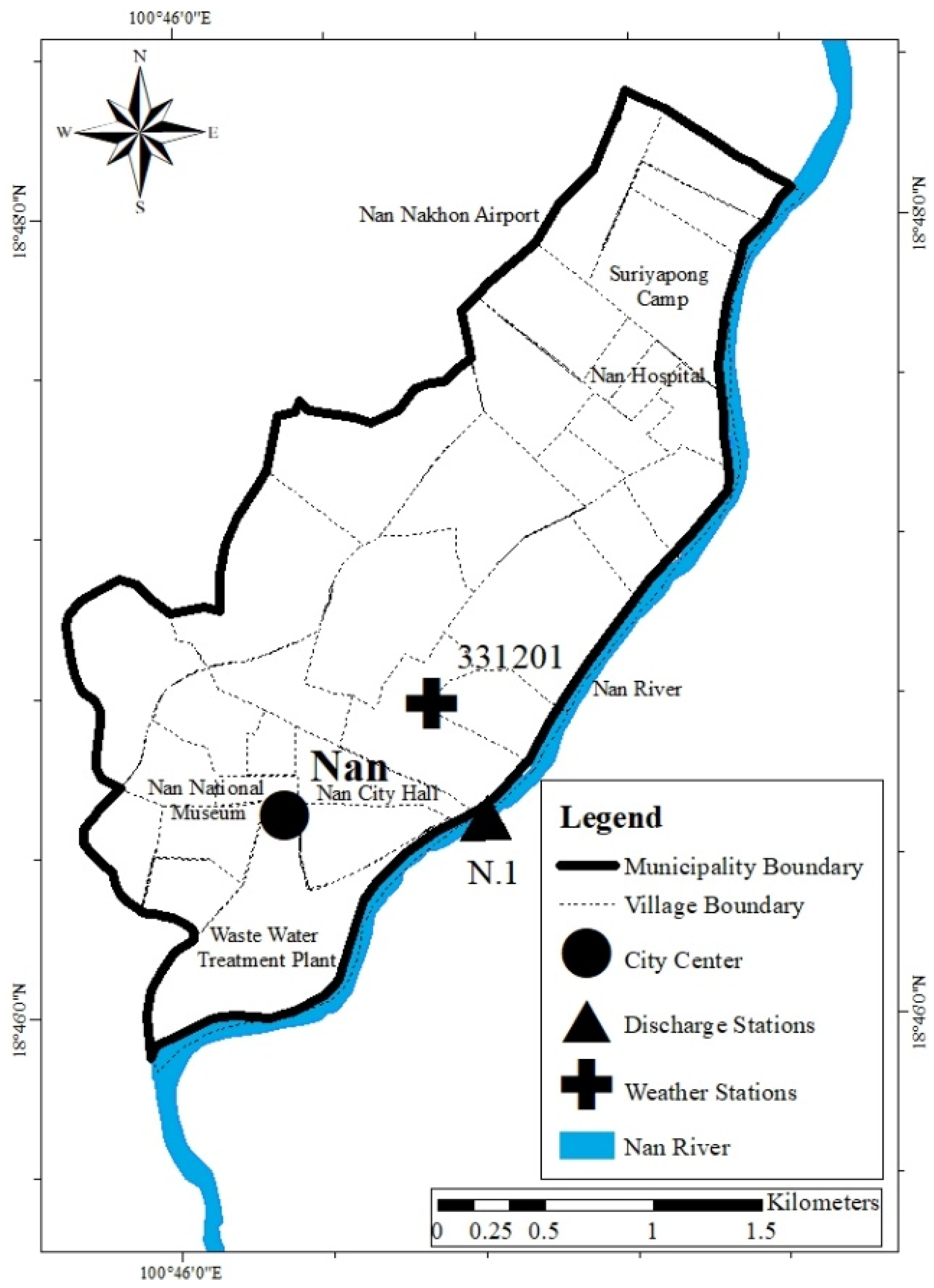
2. Study Area

The Upper Nan River Basin in Northern Thailand has a drainage area of 8709.50 km² [26]. Its main drainage way is the Nan River. It has an annual average temperature of 26.3 °C, relative humidity of 75.9%, wind speed of 0.9 knots, evaporation of 1457.4 mm, and rainfall of 1371 mm.

The basin drainage area from the river gauging station (N1) at Nan Province up to its headwater boundary of the river basin has an area of 5663 km² [27]. Another river gauging station upstream of station N1 is the Tha Wang Pha station (N64). The basin study area is subdivided into five sub-basins, namely, Upper Nan, Nam Yao (W), Nam Yao (E), Nam Samun, and Nam Nan part-2 as shown in Figure 2 [28].

These five sub-basins contribute runoff to the Nan River which flows from north to south through Nan’s municipal area of 7.6 km² on the right bank of the Nan River as shown in Figure 3. The municipal area is an urban area that has 31 villages that are mainly residential. The Nan River flows through the municipal area for a distance of 7 km. In this river reach, overbank flow occurs frequently during high flood periods. The municipal area has flooded often in the past. Large flood inundations occurred in 2006 [29] and 2011 due to the fact of heavy tropical storms [30]. Considerable flood damages and casualties were reported in both years.

3. Research Structure and Methodology

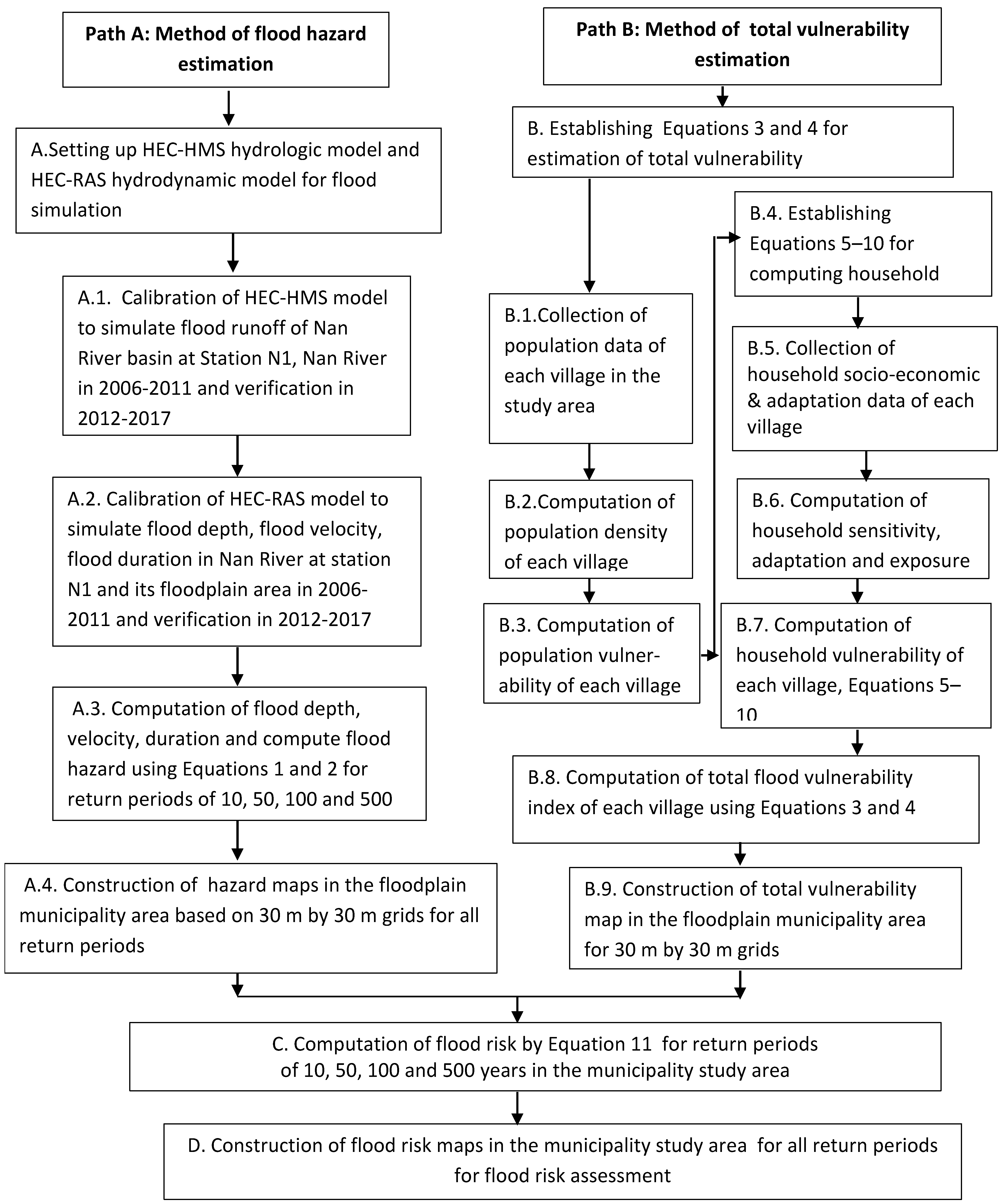
3.1. Research Structure

The research structure and methodology of this study is well described in Figure 4. The research structure has two parallel paths: Path A for flood hazard estimation and Path B for vulnerability estimation. The flow of work in Path A is from Block A.1 to Block A.4 as shown in the figure. The flow of work in Path B is from Block B.1 to Block B.9. The output of Block A.1, or flood hazard, and the output of Block B.9, or vulnerability, are multiplied to obtain the flood risk as shown in Block C near the bottom of the figure. The flood risk maps are constructed, as shown in Block D, based on the computed flood risk in Block C. From here onward, flood risk analysis and assessment were carried out to obtain a risk reference for further evaluation of risk reduction of proposed flood control measures. The methodology for the computational flood hazard, vulnerability, and flood risk analysis is described in detail in the following section.

3.2. Methodology

3.2.1. Determination of Flood Hazard

The flood hazard index (FHI) is expressed by Equation (1) in which FHIT is the flood duration index, FHID is the flood depth index, and FHIV is the flood flow velocity index. The symbols α, β, and µ are their weighting factors, respectively.

$$\mathrm{FHI}=\mathsf{\alpha } \mathrm{FHIT}+\mathsf{\beta } \mathrm{FHID}+\mathsf{\mu } \mathrm{FHIV}$$

(1)

where

$$\mathsf{\alpha }+\mathsf{\beta }+\mathsf{\mu }=1$$

(2)

The values for FHIT, FHID, and FHIV are determined according to the specified ranges of the computed flood duration, flood depth, and flood velocity in the study area as shown in

Table 1. Classification of flood hazard parameters, hazard levels, and hazard indices.

Hazard Parameters	Hazard Level	Hazard Index
Flood Duration, T (h)		FHIT
T ≤ 60	Very Low	1
60 < T ≤ 100	Low	2
100 < T ≤ 120	Medium	3
120 < T ≤ 140	High	4
140 < T	Very High	5
Flood Depth, D (m)		FHID
D ≤ 0.60	Very Low	1
0.60 < D ≤ 2.00	Low	2
2.00 < D ≤ 2.25	Medium	3
2.25 < D ≤ 2.50	High	4
2.50 < D	Very High	5
Flood Velocity, V (m/s)		FHIV
V ≤ 0.10	Very Low	1
0.10 < V ≤ 0.50	Low	2
0.50 < V ≤ 0.60	Medium	3
0.60 < V ≤ 0.70	High	4
0.70 < V	Very High	5

. The computed flood duration is classified into five ranges: very low, low, medium, high, and very high as shown in Table 1. The corresponding FHIT of each class is specified as 1, 2, 3, 4, and 5, respectively. The same method is applied to the FHID and FHIV. The sum of the weights α, β, and µ is equal 1. The weights α, β, and µ are determined using the analytic hierarchy process (AHP) of multi-criteria decision analysis [24,25,31,32,33] based on field and questionnaire surveys. The details of determining α, β, and µ by using AHP is explained in the Appendix A. Finally, the hazard level of FHI is specified as very low when FHI ≤ 1, low when 1 < FHI ≤ 2, medium when 2 < FHI ≤ 3, high when 3 < FHI ≤ 4, and very high when 4 < FHI ≤ 5.

3.2.2. Determination of Total Flood Damage Vulnerability

The total flood damage vulnerability index (FVI) for each village is calculated as the sum of the weighted flood vulnerability index of the population, FVI_pop, and the weighted flood vulnerability index of households, FVI_hh. The total vulnerability index (FVI) of each village is calculated by the following equations:

$${\mathrm{FVI}=\mathrm{w}}_{\mathrm{pop} }{\mathrm{FVI}}_{\mathrm{pop}}{+\mathrm{w}}_{\mathrm{hh}}{\mathrm{FVI}}_{\mathrm{hh}}$$

(3)

$${\mathrm{w}}_{\mathrm{pop}}{+\mathrm{w}}_{\mathrm{hh} }=1$$

(4)

The weights w_pop and w_hh are determined using AHP. The level of total vulnerability FVI is specified as very low when FVI ≤ 1, low when 1 < FVI ≤ 2, medium when 2 < FVI ≤ 3, high when 3 < FVI ≤ 4, and very high when 4 < FVI ≤ 5.

In determining FVI_pop, population vulnerability, VI_pop, is represented by population density (person/km²) and is classified into five ranges in ascending order as given in

Table 2. Classification of population vulnerability, household vulnerability, vulnerability levels, and indices.

Range of Population Vulnerability, VIpop (Person/km2)	Vulnerability Level	FVIpop Index
VIpop ≤ 1000	Very Low	1
1000 < VIpop ≤ 2000	Low	2
2000 < VIpop ≤ 3000	Medium	3
3000 <VIpop ≤ 4000	High	4
4000 < VIpop	Very High	5
Range of Household Vulnerability, VIhh(Equation (5))	VulnerabilityLevel	FVIhh Index
VIhh ≤ 22.6	Very Low	1
22.6 < VIhh ≤ 29.2	Low	2
29.2 < VIhh ≤ 35.8	Medium	3
35.8 < VIhh ≤ 42.4	High	4
42.4 < VIhh	Very High	5

. These five ranges are represented by the integer numbers 1, 2, 3, 4, and 5 for the index FVI_pop: very low, low, medium, high, and very high respectively. The household vulnerability index, FVI_hh, is determined by the value of the household vulnerability. VI_hh and its ranges according to Table 2. The VI_hh of the household samples is expressed as a function of three major contributing factors, namely: sensitivity F1, adaptive capacity F2, and exposure F3 according to the following equation:

$${\mathrm{VI}}_{\mathrm{hh}}=\left[{\mathrm{w}}_3{\mathrm{F}3-\mathrm{w}}_2\mathrm{F}2\right]{\mathrm{w}}_1\mathrm{F}1$$

(5)

$${\mathrm{w}}_1{ + \mathrm{w}}_{2 }{+ \mathrm{w}}_3 = 1$$

(6)

where w₁, w₂, and w₃ are the weights of F1, F2, and F3, respectively. The major contributing factors F1, F2, and F3 are defined in [24,25]. Equation (5) was developed in this study based on the original equation in [34,35,36] by including the weights w₁, w₂, and w₃ in Equation (5). The weighting factors w₁, w₂, and w₃ were introduced to normalize the relative importance of F1, F2, and F3. The values of w₁, w₂, and w₃ were determined by the AHP using data from collected samples of questionnaires and field surveys. Equation (6) requires that the sum of the weighting factors w₁, w₂ and w₃ is equal to one.

Each major contributing factor is divided into various components in which each component is further classified into sub-classes. An impact score is assigned to each class, as shown in

Table 3. Major contributing factors of household vulnerability and their components in Phumin-Thali village.

Major Con-tributing Factors Fi in Equations (5) and (6)	Weights Wi of Fi in Equations (5) and (6)	Components Ci of Factor Fi in Equation (7) & Definitions	Classification of Component Ci in Equation (7) into j Classes and Their Ranges	% of Total Collected Samples	Impact Score Kj of Class j in % in Equation (8)	Weights θi of Ci in Equations (8) and (9)	Remarks on Definition of Each Class of Ci
F1 = Sensitivity	W1 = 0.26	C1 = family size	Class 1 = family members > 5; Class 2 = members between 3–5; Class 3 = less than 3	Q1 = 16.7 Q2 = 33.3 Q3 = 66.7	100 67 33	θ1 = 0.386	Larger family is more sensitive to flooding
		C2 = gender of householder	Class 1 = female; Class 2 = male	Q1 = 33.3 Q2 = 66.7	100 40	θ2 = 0.193	Female is more sensitive to flooding than male
		C3 = health of householder	Class 1 = very poor; Class 2 = poor; Class 3 = good; Class 4 = very good	Q1 = 0 Q2 = 16.7 Q3 = 50.0 Q4 = 33.3	100 75 50 25	θ3 = 0.129	Very poor health person is most sensitive to flooding
		C4 = land use type	Class 1 = houses + orchards; Class 2 = houses + shops; Class 3 = houses only	Q1 = 0 Q2 = 50 Q3 = 50	100 67 33	θ4 = 0.055	House + orchard land is most vulnerable and most sensitive to flooding
		C5 = household damages, THB	Class 1 = damages >10,000; Class 2 = damages 5000–10,000; Class 3 = damages <5000; Class 4 = no damage	Q1 = 0 Q2 = 33.3 Q3 = 16.7 Q4 = 50.0	100 75 50 25	θ5 = 0.096	Household with higher damage potential is more sensitive to flooding
		C6 = public damages (THB/m2)	Class 1 = damages >750; Class 2 = damages 750–501; Class 3 = 501–250; Class 4 = less than 250	Q1 = 0 Q2 = 100 Q3 = 0 Q4 = 0	100 75 50 25	θ6 = 0.077	Public property of higher damages is more sensitive to flooding
		C7 = household ownership	Class 1 = owner; Class 2 = tenant	Q1 = 66.7 Q2 = 33.3	100 0	θ7 = 0.064	Owners are more sensitive to flooding than tenants
F2 = Adaptive Capacity	W2 = 0.11	C1 = education level of householder	Class 1 = university; Class 2 = higher secondary; Class 3 = secondary; Class 4 = primary; Class 5 = illiterate	Q1 = 16.7 Q2 = 33.3 Q3 = 0 Q4 = 50.0 Q5 = 0	100 80 60 40 20	θ1 = 0.129	Higher educated person has more adaptive capacity to flooding
		C2 = type of employment of householder	Class 1 = Govt. officer; Class 2 = private worker; Class 3 = agriculture; Class 4 = daily wage Class 5 = unemployed	Q1 = 16.7 Q2 = 0 Q3 = 0 Q4 = 83.3 Q5 = 0	100 80 60 40 20	θ2 = 0.096	Government officer has highest adaptive capacity to flooding
		C3 = householder income (THB/month)	Class 1 = income >25,000; Class 2 = income 25,000–20,001; Class 3 = 20,000–15,001; Class 4 = 15,000–10,001; Class 5 = 10,000–5001; Class 6 = less than 5000	Q1 = 16.7 Q2 = 16.7 Q3 = 0 Q4 = 16.7 Q5 = 16.7 Q6 = 33.3	100 83 67 50 33 16.7	θ3 = 0.386	Householder with higher income has more adaptive capacity to flooding
		C4 = household saving deposit	Class 1 = yes; Class 2 = no	Q1 = 100 Q2 = 0	100 0	θ4 = 0.193	Household with saving deposit has more adaptive capacity
		C5 = flood insurance	Class 1 = yes; Class 2 = no	Q1 = 0 Q2 = 100	100 0	θ5 = 0.055	Household with flood insurance has more adaptive capacity
		C6 = land price (THB/m2)	Class 1 = land price >7500 Class 2 = 7500–5001; Class 3 = 5000–2501; Class 4 = 1–2500	Q1 = 0 Q2 = 0 Q3 = 100 Q4 = 0	100 75 50 25	θ6 = 0.064	Household in high price land is richer and has more adaptive capacity
		C7 = flood notification	Class 1 = yes; Class 2 = no	Q1 = 100 Q2 = 0	100 0	θ7 = 0.077	People with flood notification have more adaptive capacity
F3 = Exposure	W3 = 0.63	C1 = distance from river, m	Class 1 = distance <500, Class 2 = 501–1000; Class 3 = 1001–1500; Class 4 = 1501–2000; Class 5 = more than 2000	Q1 = 100 Q2 = 0 Q3 = 0 Q4 = 0 Q5 = 0	100 80 60 40 20	θ1 = 0.408	Area at shorter distance to river is more exposed to flooding
		C2 = ground elevation, m	Class 1 = elev. 190–195, Class 2 = 196–200, Class 3 = 201–205, Class 4 = 206–210, Class 5 = elev.211–215	Q1 = 100 Q2 = 0 Q3 = 0 Q4 = 0 Q5 = 0	100 80 60 40 20	θ2 = 0.204	Area with lower elevation is more exposed to flooding
		C3 = inundation depth in 2011, m	Class 1 = depth >2.0; Class 2 = 1.1- 2.0; Class 3 = 0.1–1.0; Class 4 = less than 0.1	Q1 = 0 Q2 = 83.3 Q3 = 16.7 Q4 = 0	100 75 50 25	θ3 = 0.102	Area having larger inundation depth is more exposed to flooding
		C4 = flood velocity in 2011, ms−1	Class 1 = velocity >2.0; Class 2 = 1.1–2.0; Class 3 = 0.1–1.0; Class 4 = less than 0.1	Q1 = 16.7 Q2 = 50 Q3 = 33.3 Q4 = 0	100 75 50 25	θ4 = 0.082	Area having higher flood flow velocity is more exposed to flooding
		C5 = duration of inundation in 2011, days	Class 1 = duration > 7; Class 2 = 3.5–7; Class 3 = 0.5–3.5; Class 4 = less than 0.5	Q1 = 0 Q2 = 50 Q3 = 50 Q4 = 0	100 75 50 25	θ5 = 0.136	Area having longer flood duration is more exposed to flooding
		C6 = number of flooding events in 2011	Class 1 = 3 flooding events or more; Class 2 = 2 flooding events; Class 3 = 1 flooding event; Class 4 = none	Q1 = 0 Q2 = 33.3 Q3 = 66.7 Q4 = 0	100 75 50 25	θ6 = 0.068	Area having more frequent flooding is more vulnerable to flooding

, according to the influence or impact of the class on its component.

For example, the sensitivity F1 is further classified into 7 contributing components C₁–₇ in which C₁ = family size, C₂ = gender, C₃ = health, C₄ = land use type, C₅ = household damage, C₆ = public property damages, and C₇ = ownership of household. The sensitivity F1 is computed as:

$$\mathrm{F}1={\sum }_{\mathrm{i}=1}^{\mathrm{n}=7}{\mathrm{C}}_{\mathrm{i}}$$

(7)

where C_i is the ith contributing component of the sensitivity factor F1, and n = 7 is the total number of the component C_i of F1.

Each contributing component C_i of F1 is computed as:

$${\mathrm{C}}_{\mathrm{i}}={\mathsf{\theta }}_{\mathrm{i}}{\displaystyle \sum }_{\mathrm{j}=1}^{\mathrm{m}}{\mathrm{Q}}_{\mathrm{j}}{\mathrm{K}}_{\mathrm{j}}$$

(8)

$${{\displaystyle \sum }}_{\mathrm{i}=1}^{\mathrm{n}=7}{\mathsf{\theta }}_{\mathrm{i}}=1$$

(9)

where the weight θ_i of C_i is determined by AHP based on the collected samples from questionnaires and field surveys; m is the number of classes of the collected samples for the component C_i, arranged from the highest to the lowest significance of vulnerability; Q_j is the number of samples of class j as a percentage of the total collected samples of all classes; K_j is the assigned impact score of the class j between 0% and 100%. A score of 100% is assigned to the class that has the highest impact on vulnerability. More details regarding the calculation are given in the next section on the computational procedure.

The component C₁ for F1 is calculated as follows:

$${\mathrm{C}}_1{=\mathsf{\theta }}_1{\displaystyle \sum }_{\mathrm{j}=1}^3{\mathrm{Q}}_{\mathrm{j}}{\mathrm{K}}_{\mathrm{j}}$$

(10)

where Q_j is the number of family samples in the jth class with the assigned impact score K_j, and θ₁ is the weight of C₁ to be determined by AHP.

The same overall procedure described above is applied to the other two major contributing factors, namely: adaptation F2 and exposure F3. For the adaptation capacity F2, there are seven components as shown in Table 3, namely: education level of householders, their employment, household income, saving deposit, insurance for flood events, land price, and notification of flood events.

The exposure F3 in Table 3 is composed of six major components, namely: the distance from the river, ground elevation, the inundation depth in 2011, the flood velocity in 2011, the duration of inundation in 2011, and the number of flooding events in 2011. The year 2011 was the only year that flood inundation data in the study area were available. The exposure factor F3 was calculated based on the sum of its weighted components in which the weights were determined using AHP.

After obtaining the values of the three major contributing factors, namely, sensitivity F1, adaptation F2, and exposure F3, they were substituted into Equation (5) to calculate household vulnerability, VI_hh. The computed household vulnerability, VI_hh, of each village was fitted into the five classified ranges: very low, low, medium, high, and very high as shown in Table 2. Then, the value of FVI_hh corresponding to VI_hh was represented by an integer number from 1 to 5 according to Table 2.

Finally, the vulnerability indices of population density, FVI_pop, and of household FVI_hh were substituted into Equation (3) to compute the total vulnerability, VI.

Each village area occupies many grids of 30 by 30 m, which are used in calculating the flood hazard. As the grid size is relatively much smaller than the area of each village, all the grids in the same village are considered to have the same value of the total vulnerability, FVI.

3.2.3. Determination of Flood Risk

By using the same grids for hazard and vulnerability, the flood risk index, FRI, for each grid in the study area was computed as the product of the FHI and the total flood damage vulnerability index, FVI. The flood risk index (FRI) is calculated as:

$$\mathrm{FRI}=\mathrm{FHI} \times \mathrm{FVI}$$

(11)

Equation (11) does not explicitly include exposure. This is different from the equation given in [16], which includes exposure. In this study, exposure data were collected from the questionnaires and field surveys as shown in Table 3. This exposure term, F3, was considered in Equation (5) when calculating household vulnerability, V_hh, and the total vulnerability, FVI. The computed values of the FRI were classified into five ranges corresponding to very low for 1 < FRI ≤ 5, low for 5 < FRI ≤10, medium for 10 < FRI ≤ 15, high for 15 < FRI ≤ 20, and very high for 20 < FRI ≤ 25.

3.3. Data Collection

3.3.1. Hydrological Data

For the hydrological model simulation and the hydrodynamic model simulation, the hourly hydro-meteorological data from four stations (i.e., 331201, 331301, 331401, and 331402), as shown in Figure 2, and the daily river discharge and water level data at two stations at N1 (Nan) and N64 (Tha Wang Pha) were collected from the regional offices of the Thai Meteorological Department and of the Royal Irrigation Department (RID), Thailand. The river cross-sections, floodplain geometry, land topography, and DEM were collected from the Nan Provincial Office, the Regional Office of the Royal Irrigation Department (RID), and from the Geo-Informatics and Space Technology Development Agency (GISTDA).

3.3.2. Vulnerability Data

The following data were collected for the analysis: (a) land-use maps in the Nan River Basin from the Land Development Department (LDD); (b) population data and household flood damage and public infrastructure damage date in Nan Municipality from the Nan Provincial Administration; (c) socioeconomic and household data were collected from field and questionnaire surveys in the study area. The number of household samples collected for the questionnaire survey was estimated using Yamane’s equation [37]:

$$\mathrm{n}=\frac{\mathrm{N}}{{1+\mathrm{Ne}}^2}$$

(12)

where n is the number of household samples; N is the total number of households in the study area, which was 6310; e is the allowable error taken equal to 10%. The value of n was calculated and found to be approximately 100.

3.4. Computational Procedure

3.4.1. Computation of Flood Hazard

The HEC-HMS rainfall–runoff model and the HEC-RAS flood routing model are connected as shown in Figure 5 in computing flood discharges and depths. The computational procedure is as follows:

(a)

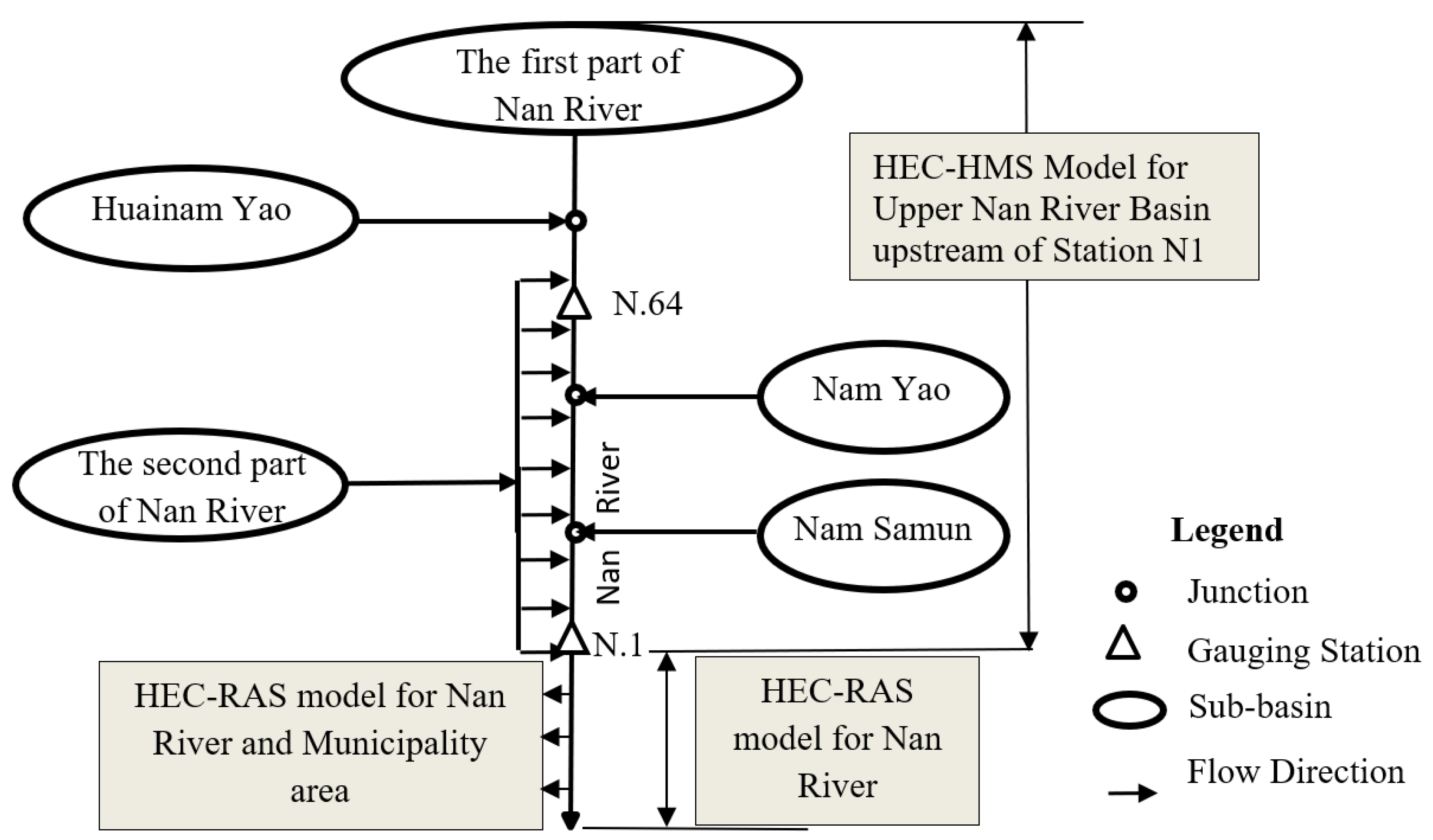
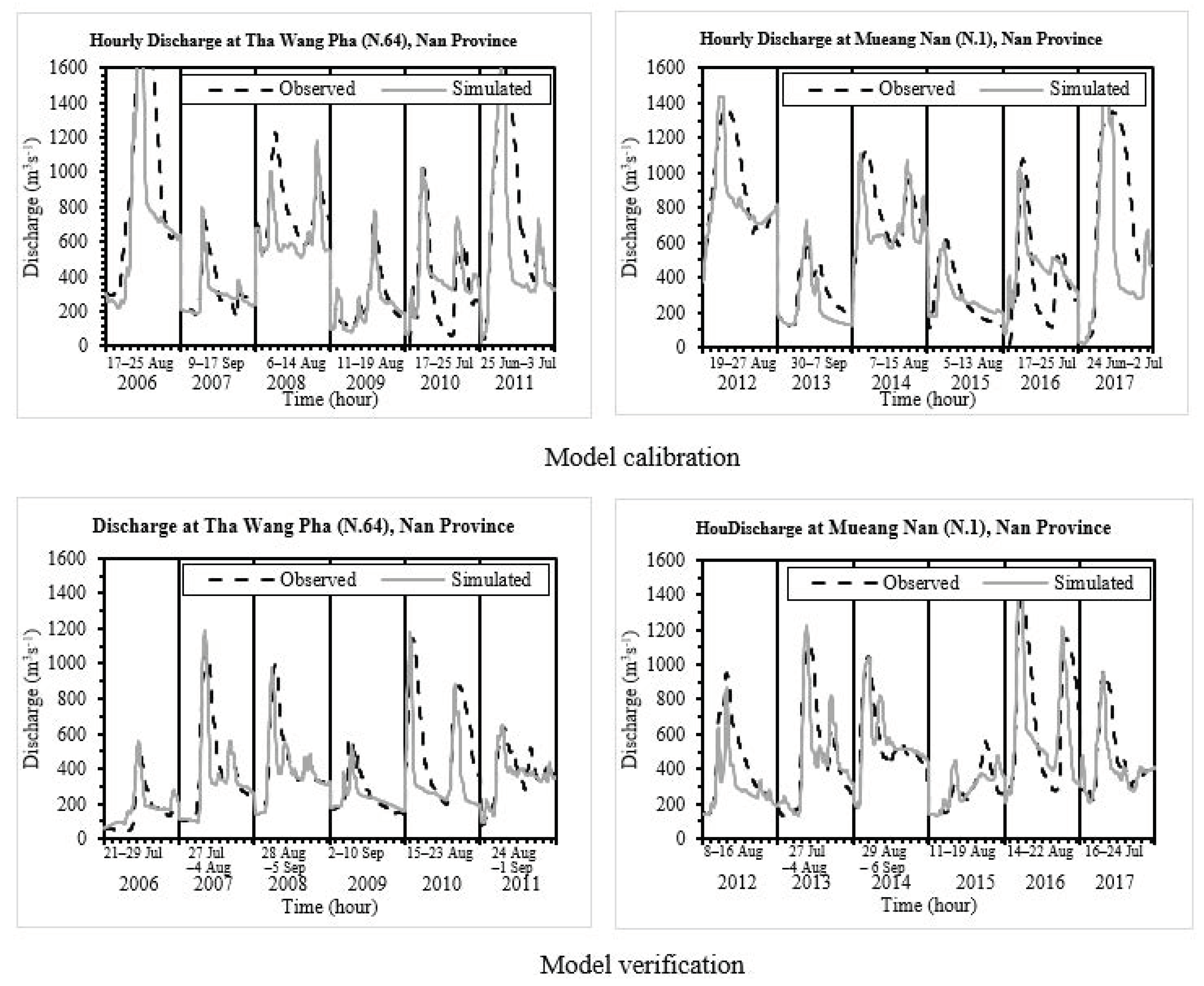
Rainfall–runoff computation: The HEC-HMS rainfall–runoff model [38] was applied to compute the runoff hydrograph using hourly rainfall input at four stations in the Upper Nan Basin. The hourly rainfalls at the four stations were averaged over the basin area using the Thiessen polygon method. The river basin was divided into seven sub-basins in which the hourly average rainfalls were used in each sub-basin. The computed runoff was used as the upstream boundary condition of the HEC-RAS flood routing model [39]. The HEC-HMS model requires a digital elevation model (DEM), soil and land-use maps, soil characteristics, and input rainfall hyetographs. The HEC–Geo HMS model, which is an extension of HEC-HMS, prepares raster layers of delineated sub-basins and river network systems for exporting to HEC-HMS as base maps. By inputting rainfall data, land cover, and soil maps to HEC-HMS, the model computes daily runoff hydrographs for each sub-basin. The HEC-HMS model was calibrated and verified against the observed daily discharges at station N64 at Tha Wang Pha and at station N1 at Muang Nan. The calibration period was during the wet period from June to December 2006–2011, and the verification period was from June to December 2012–2017. In the model calibration, the model parameters, such as initial and maximum storages of canopy, SCS curve number, time of concentration, and lag of unit hydrograph, were assumed and adjusted by trial and error to obtain a satisfactory agreement between the observed and computed discharge hydrographs;

(b)

Flood routing computation: The 1D and 2D HEC-RAS flood routing model [39] for the Upper Nan River and its floodplain were used to route the runoff from the upstream station N1 along the Nan River to the downstream end station, which is 7 km downstream of station N1. The river passes through the municipal area, which is in the river floodplain. The geometrical inputs to HEC-RAS were the measured river cross-sections every 1.2 km and the floodplain topography from the digital elevation model with a 30 by 30 m resolution with a 1 m contour interval. The river cross-sections from the field measurements and the floodplain topography from the DEM were merged using HEC-GEO RAS, an extension of HEC-RAS, to obtain the complete river and floodplain cross-sections [40]. This geometry data was input into HEC-RAS for flood flow simulation. In the HEC-RAS model, the 1D flow routing procedure was used to compute the 1D flow in the Nan River, and the 2D flow routing was used to compute the 2D flow in the floodplain;

(c)

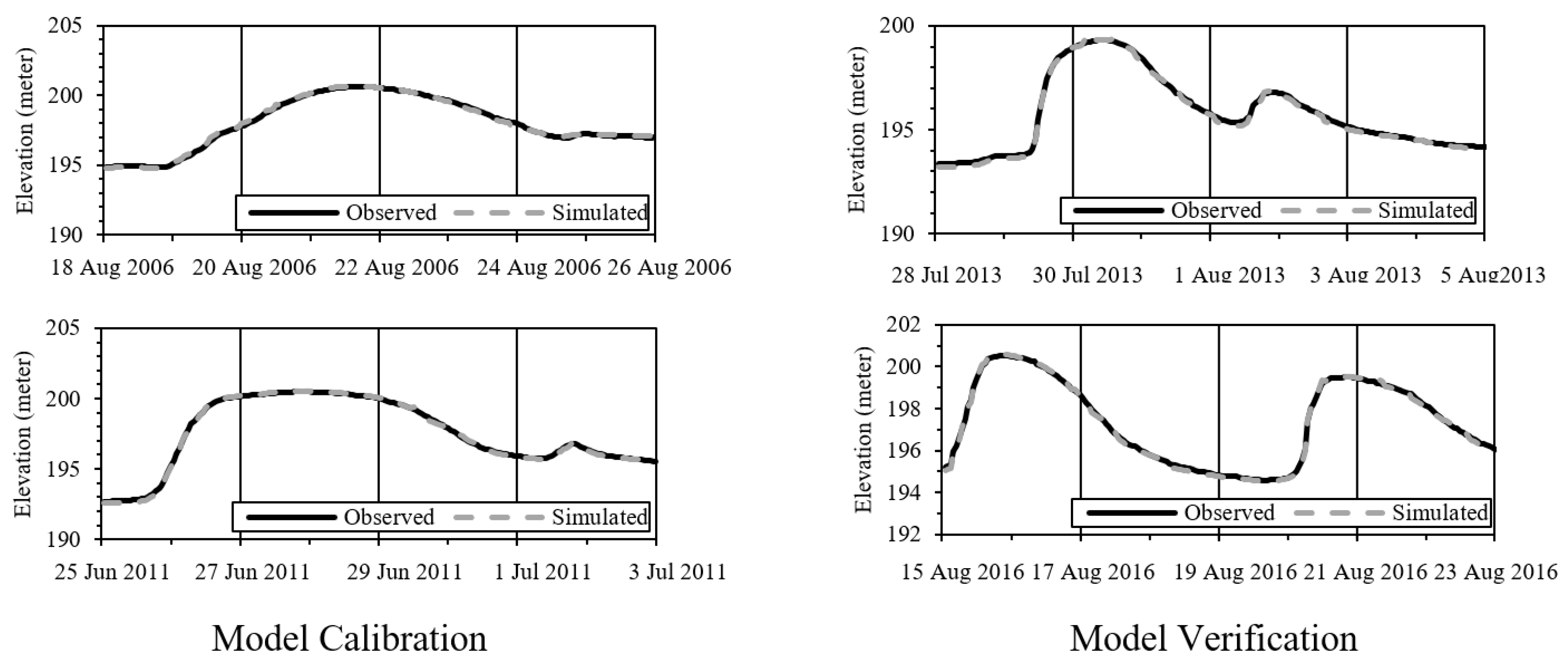
The hydrological inputs to HEC-RAS were the observed daily upstream discharge at station N1 as the upstream boundary condition. At the downstream end of the model, there was no river gauging station; thus, a depth–discharge relationship according to the Manning equation was used. The model was calibrated and verified by trial-and-error adjustment based on the values of the Manning roughness coefficient n;

(d)

Calculation of flood hazard index: The FHI was computed for each grid of 30 × 30 m in the municipality’s floodplain area using Equation (1). The flood duration index (FHI_T), the depth index (FHI_D), and the velocity index (FHI_V) were determined by using the results of the HEC-RAS model and the classification in Table 3. As shown in Figure 4, for Blocks A.1 to A.4, the computed FHI_D, FHI_V, and FHI_T were substituted into Equation (1) to compute the FHI. The hazard weighting factors α for flood duration, β for flood depth, and µ for flood velocity in Equation (1) were determined using AHP [24,25].

3.4.2. Computation of Total Vulnerability

As shown in Figure 4, for Blocks B.1 to B.8, the total vulnerability of the study area was computed as a function of the vulnerability of the population and the vulnerability of households. According to Equations (3) and (4), the total vulnerability is equal to the sum of the weighted vulnerability of the population and the weighted vulnerability of households. The weights of the vulnerability of the population and of household vulnerability were determined using AHP based on the questionnaire surveys.

The vulnerability of the population of each village was computed from the population density (number of persons/km²) of each village from census data. For the household vulnerability, VI_hh, each major contributing factor of VI_hh was composed of a number of components in which each component was further subdivided into classes with assigned impact scores. For example, the major contributing factor F1, or sensitivity, had seven components (C₁–₇), namely: family size, gender, health, land-use type, household damage, public damage, and household ownership as shown in Table 3. An example of calculating the component C₁ or family size of F1 in Table 3 for Phumin-Thali village is given here. The family size was subdivided into three classes: class 1 for households with more than five family members; class 2 for between three and five family members; class 3 for fewer than three family members. The impact scores of 100%, 67%, and 33% were assigned to each family class according to the information from local residents on vulnerability to their families. A score of 100% was assigned to class 1, because it is most sensitive to vulnerability. The number of collected household samples in Phumin-Thali village was six.

The component C₁ of the major contributing factor F1 was classified into three classes (m = 3). In class 1 (j = 1), the number of the families was equal to one. Hence, Q₁ was equal to 16.67% of the total collected samples of six, and the impact score K₁ was assigned to be 100%. In class 2 (j = 2), the number of families was equal to two or Q₂ = 33.33% and assigned K₂ = 67%. In class 3 (j = 3), the number of families was three or Q₃ = 50% and K₃ = 33%. The weighting factor θ₁ of the sensitivity factor F1 was determined by AHP and equal to 0.386. This is shown at the beginning of Table 3. Knowing Q₁, Q₂, Q₃, K₁, K₂, K₃, and θ₁, the value of the component C₁ of F1 is equal to θ₁ (Q₁K₁ + Q₂K₂ + Q₃K₃)/100 = 21.41%.

The same procedure was repeated for the remaining classes 2 and 3 of the component C₁ of the factor F1 as shown in Table 3. In this way, the components C₁–₇ were calculated using Equation (8) and summed to obtain the major contributing factor F1 according to Equation (7).

The same overall procedure was repeated for the major contributing factors F2 and F3. Hence, the total vulnerability, VI, and its index, FVI, was determined from Equations (3) and (4).

3.4.3. Computation of Flood Risk

As shown in Figure 4, the FRI was computed as the product of the FHI and the FVI. The distribution of flood risk over the municipal area can be represented by a flood risk map of grids of 30 by 30 m resolution. The maps of flood hazard and risk of a spatial resolution of 30 × 30 m were constructed for 10, 50, 100, and 500 year return periods. The flood risk index of each grid for each return period was classified into five levels of equal intervals, namely: very low for 1 < FRI ≤ 5, low for 5 < FRI ≤ 10, medium for 10 < FRI ≤ 15, high for 15 < FRI ≤ 20, and very high for 20 < FRI ≤ 25.

4. Results

4.1. Calibration and Verification of the HEC-HMS Rainfall–Runoff Model and HEC-RAS Flood Routing Model

The HEC-HMS rainfall–runoff model, which covers the Upper Nan River Basin area from its headwater to the model outlet at the gauging station N1, was calibrated and verified against the observed daily discharges at gauging stations N64 at Tha Wang Pha and N1 at Mueang Nan. The calibration period was during the wet period from June to December in 2006–2011, and the verification period was from June to December in 2012–2017. In the model’s calibration, the model parameters, such as initial and maximum storages of canopy, SCS curve number, time of concentration, and lag of unit hydrograph, were assumed based on previous studies [21,40] and adjusted by trial and error to obtain a satisfactory agreement between the observed and computed discharge hydrographs (Figure 6). The model’s performance was evaluated using the following statistical parameters, namely: coefficient of determination (R²), Nash–Sutcliffe efficiency (NSE), percent bias (PBIAS), volume ratio (Vr), and normalized root mean square error (NRMSE). The results of the model’s calibration at stations N64 and N1 were found to be satisfactory with coefficients of determination of 0.72 and 0.76; Nash–Sutcliffe efficiencies of 0.67 and 0.64; percent biases of 15.78 and 15.11; volume ratios of 0.95 and 0.89; normalized root mean square errors of 12.29% and 14.36%, respectively. The statistics showed acceptable agreement in both the model’s calibration and verification.

The HEC-RAS flood routing model covers the Nan River reach from the river gauging station N1 to the downstream end station 7 km downstream and its floodplain in the municipal area. The model was calibrated by comparing the computed and observed daily water levels at station N1 during the peak flood periods in 2006–2011, while in the floodplain, there was no water level data. According to [41], the Manning roughness coefficient n of 0.03 was initially assumed for the river and its floodplain in the calibration. The assumed Manning roughness coefficients were adjusted by trial and error and were found to be 0.032 for the river and 0.035 for the floodplain. These Manning n values matched with the roughness condition of the river channel and its floodplain, which is moderately rough according to [9]. The model was verified with the observed flood water levels at the river gauging station N1 during the flood periods in 2012–2017. The values of the performance statistics of both the model’s calibration and verification were as follows: coefficient of determination of 0.97 and 0.95; Nash–Sutcliffe efficiencies of 0.89 and 0.80; percent biases of 24 and 38; volume ratios of 1.0 and 1.0; normalized root mean square errors of 7.36% and 11.16%, respectively. The statistics showed acceptable agreement for both the model’s calibration and verification. The computed maximum flood water levels and discharges in the municipality’s floodplain area downstream of station N1 were compared with the measured high-water marks. The model was successfully calibrated and verified as shown in Figure 7.

The results of the calibration and verification of the HEC-RAS model for the river flow during flood peak periods are shown in Figure 7. As shown in the results, the performance statistics showed acceptable agreement for both the model’s calibration and verification. The comparison of the computed and observed inundation depths of high-water marks in the floodplain at the three locations, namely, Phuang-Payom, Phumin-Thali, and Mueang Len, were found to be satisfactory with percentage errors of 6.7, 6.3, and 9.1, respectively. This assures the accuracy of the model simulation in the floodplain.

The HEC-RAS model was applied to calculate the flood duration, flood depth, and flood velocity in the municipality’s floodplain area for the flood return periods of 10, 50, 100, and 500 years. It was found that the computed flood duration, T, varied from 74 to 151 h; the flood inundation depth, D, from 1.5 to 2.97 m; the flood flow velocity, V, from 0.34 to 0.81 ms⁻¹.

From the results of the HEC-RAS model, flood hazard maps of the municipal area for the return periods of 10, 50, 100, and 500 years were constructed as shown in Figure 8 and Figure 9 respectively.

4.2. Flood Hazard

In Equation (1), the flood duration index (FHIT), flood depth index (FHID), and flood velocity index (FHIV) were computed based on the results of the HEC-RAS model and the criteria in Table 2. They were substituted into Equation (1) to compute the FHI.

The hazard weighting factors α for flood duration, β for flood depth, and µ for flood velocity in Equation (1) were determined by AHP [24,25] as described in the Appendix A. It was found that weight α was 0.63 for the flood duration, β was 0.26 for the flood depth, and μ was 0.11 for the flood velocity. The sum of the three weights was equal to unity according to Equation (2).

The values of the FHI of each grid was computed for floods in the return periods of 10, 50, 100, and 500 years. In the municipal area of 7.6 km², the total flooded area for the 100 year return period was found to be 1,614,545 km², or 21.24% of the study area. The remaining part of the study area had no flood inundation. According to the ranges of classification, the hazard index of the flooded area of 1,614,545 km² was classified into a very high hazard area of 307,638 km², or 19.05% of the study area; a high hazard of 25,622 km², or 1.59%; a medium hazard of 68,432 km², or 4.32%; a low hazard of 1,014,760 km², or 62.85%; a very low hazard of 198,094 km², or 12.26%. The high and very hazardous areas were in Phumin-Thali village in the south of the study area, and another major flooding location was in the area of Suriyapong Camp in the north of the study area.

4.3. Total Flood Vulnerability

The total vulnerability index, FVI, was determined for each village using Equations (3) and (4). The computed population vulnerability index, FVI_pop, and the computed household vulnerability index, FVI_hh, were substituted into Equation (3). The weights w_pop for population vulnerability and w_hh for household vulnerability were determined using AHP based on the data collected from the Nan Municipality and from the questionnaire survey. The weights w_pop and w_hh were found to be 0.33 and 0.67, respectively. This shows that the household vulnerability, FVI_hh, has much more influence on the total vulnerability, FVI, than the population vulnerability, FVI_pop.

The computed total vulnerability index, VI, was further classified into five ranges of equal intervals corresponding to the index values FVI of 1, 2, 3, 4, and 5 and named very low, low, medium, high, and very high, respectively, as shown in Table 2. Figure 10 shows the vulnerability level of different villages in the municipal area.

As shown in Figure 10, it was found that the areas along the right bank (west bank) of the Nan River and in the southern part near Phumin-Thali village were highly vulnerable and highly sensitive to floods compared to the other parts of the municipality.

From the computed total vulnerability index, FVI, of each village, it is found that 10 villages, namely, Chiang Kang, Phumin-Thali, Pouang Phrayom, Phra Nate, Mueang Len, Tha Chang, Don Khwan, Huea Khaung, Phrayaphu, and Don Sri Saim, located near the Nan River and its tributary Chao Fa canal have very high flood vulnerability.

4.4. Flood Risk

In calculating the flood risk, the municipal area was divided into grids of 30 by 30 m. In each village in the municipality, the hazard varied from one point to another depending on the flood conditions and topography. For the total vulnerability, it was considered to be the same everywhere, as the village was the smallest unit in the questionnaire survey. The computed FRI for all grids in the same village was classified into five levels with equal intervals, namely: very low for 1 < FRI ≤ 5, low for 5 < FRI ≤ 10, medium for 10 < FRI ≤ 15, high for 15 < FRI ≤ 20, and very high for 20 < FRI ≤ 25. The maps of the computed flood risks for the 100 and 500 year return periods are shown in Figure 11 and Figure 12 respectively.

From the maps, it was found that the risk level and inundation area increased significantly by four times for the return period from 100 to 500 years. In Figure 11 and Figure 12, the highest risk areas consistently appear in the most southern part of the municipal area, near to the wastewater treatment plant, where the Phumin-Thali and Phuang-Payom villages are situated. There, the ground elevation is low; flood depth and flood duration are large; the population density and number of household properties are high. For the 100 year return period, more than half of the two villages are projected to be inundated and heavily damaged.

These two villages have the highest total vulnerability and highest hazard. Other locations with the highest or at high risk are along the right bank of the Nan River, especially in the northeastern part of the municipal area around Mueang Len village and Suriyapong Camp. The medium- and low-risk areas are in the inner part of the municipality approximately 1 or 2 km away from the riverbank. In the central part of the municipal area and in the northwestern part, the flood risk is very low or none, due to the fact of their higher ground elevations.

5. Discussions

Globally, the costs of flood losses and corresponding adaptations are generally preliminary and subject to a number of assumptions. Uncertainties are largely due to the fact of projected climate changes and estimation of flood damages as well as methodological shortcomings [42]. Options for adaptation measures and assumptions of vulnerability and exposure under various scenarios of socioeconomic conditions and physical environments are important factors in changes of flood risks. An attempt to overcome these shortcomings in risk assessments was conducted in the present study by developing a comprehensive and systematic method for flood risk assessment at the household level and to demonstrate its application in a municipal area of Nan Province in Thailand.

The discussion of the results of this study is as follows:

• The performance of the HEC-HMS model was evaluated using the following statistical parameters, namely: R², NSE, PBIAS, Vr, and NRMSE. The results of the model’s calibration at stations N64 and N1 were found to be satisfactory as shown in the results, and. the performance statistics showed acceptable agreement in both the model’s calibration and verification;
• The comparison of the computed and observed inundation depths of high-water marks in the floodplains at Phuang-Payom, Phumin-Thali, and Mueang Len villages were found to be satisfactory with percentage errors of 6.7, 6.3, and 9.1, respectively. This assures the accuracy of the model’s simulation in the floodplain. Importantly, the results show the reliability of the HEC-RAS flood simulation model and the data used in the calculation;
• The flood hazard was calculated by using Equations (1) and (2) in which the weights α, β, and μ representing flood duration, depth, and velocity, respectively, were systematically determined by AHP. In the other previous studies [17,18,20], the weights α, β, and μ for flood duration, depth, and velocity, respectively, in Equation (1) were specified by the researchers according to their experiences without using AHP. These weights could be subjective or questionable. By using the AHP, the weights α, β, and μ of 0.63, 0.26, and 0.11, respectively, were obtained. In AHP, the relative importance of a flood duration, depth, and velocity of 1, 3, and 5 was assigned according to the results of field and questionnaire surveys. A sensitivity analysis was conducted to determine the effects of change on the relative importance of flood duration, depth and, velocity from the original values of 1, 3, and 5 to the new values of 1, 5, and 9, respectively. By using AHP, the new weights α, β, and μ were found to be 0.72, 0.21 and 0.06, respectively. In percent, the changes were +14.3% for weight α, −19.2% for β, and −45.4% for μ. The changes in weights α and β were considered to be small and acceptable. The change in weight μ of −45.4% was negative and moderate. Based on the field and questionnaire surveys in this study, it was revealed that the damaging effect of flow velocity in the municipal area was much smaller compared to flood duration and depth; therefore, the change in weight μ of −45.4% was considered non-significant. Hence, weights α, β, and μ of 0.63, 0.26, and 0.11, respectively, were considered reasonable;
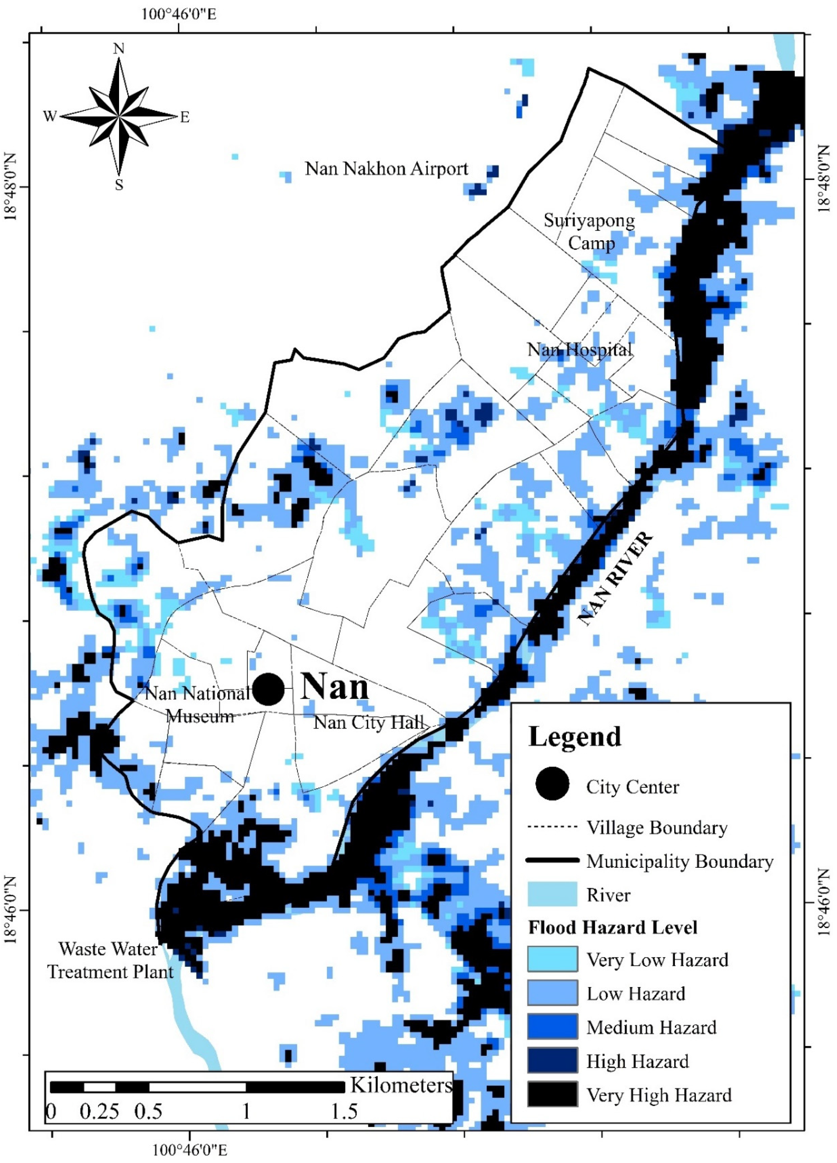
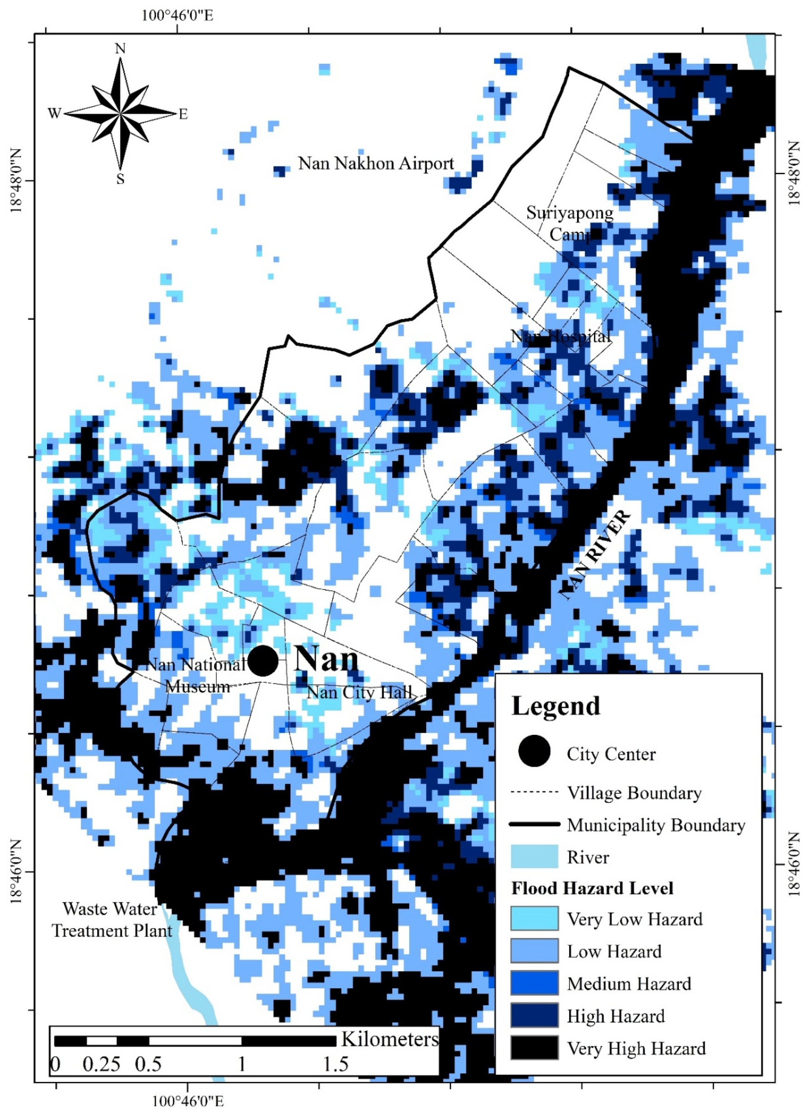
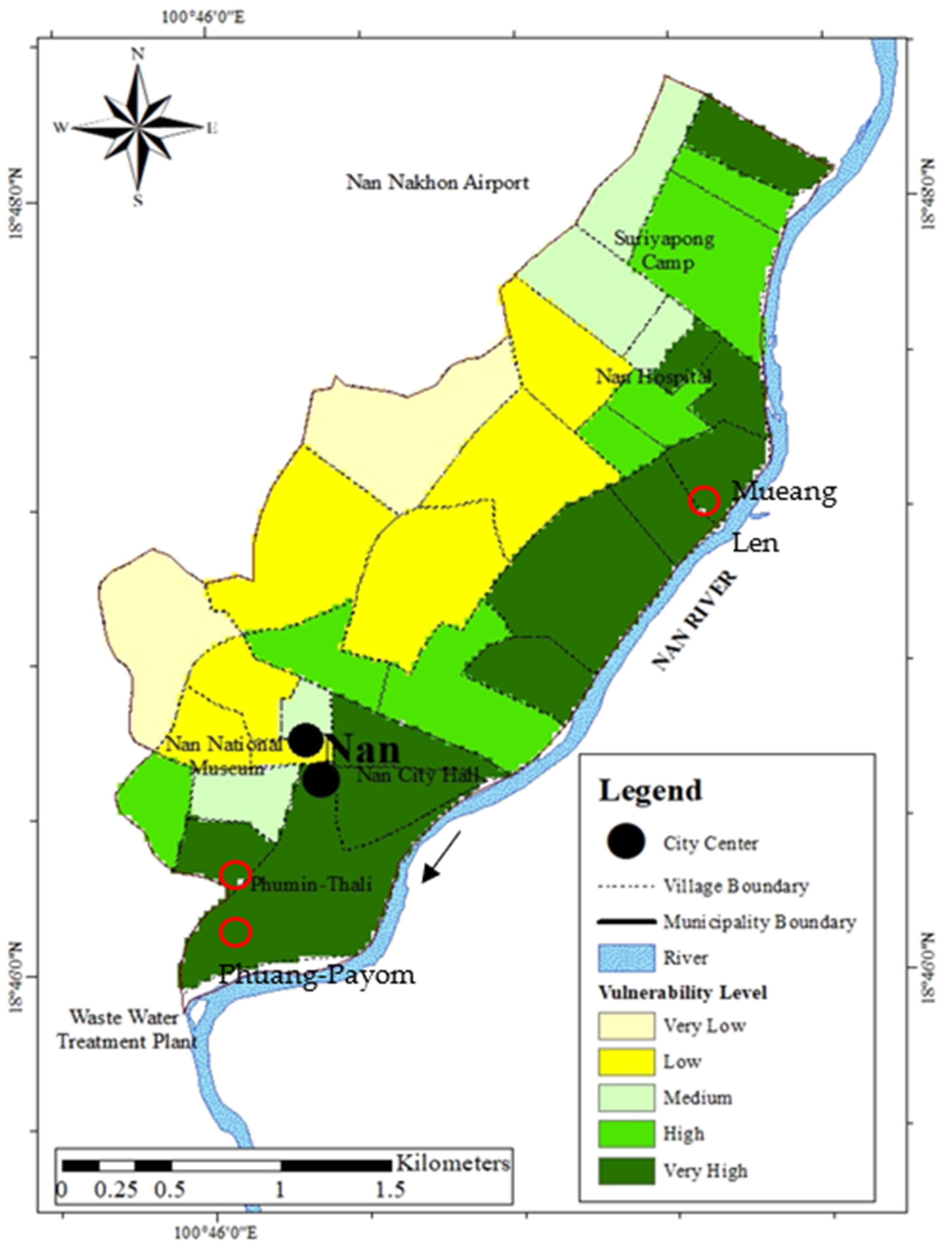
• As shown in Figure 8 and Figure 9, the flood hazard increased both spatially and in magnitude with the increase in the flood return periods. The 10 year flood hazard along the right bank of the Nan River was smaller than the 50 and 100 year floods, and it was much smaller compared to the 500 year flood. Significant flood hazard occurs in the Phumin-Thali and Phuang-Payom villages in the southern part of the municipality. The locations of the observed high-water marks are shown by the small red circles in Figure 10. It can be seen that the center of the municipal area has higher ground elevation than the surrounding area and, hence, it has less of a flood hazard. On the other hand, in the Mueang Len area in the northeastern part of the municipality, the hazard is significant when the flood magnitude is greater than the 100 year return period;
• For total flood vulnerability, the weights W_pop and W_hh in Equation (3) were found to be 0.33 and 0.67, respectively. This shows that FVI_hh had much more influence on FVI than FVI_pop. For household vulnerability, FVI_hh, the relative importance of the major contributing factors, namely, sensitivity F1, adaptation F₂, and exposure F₃ were set to be 1, 3, and 5, respectively. By using AHP, the weights of w₁ of sensitivity F1, w₂ of adaptation F2, and w₃ of exposure F3 were found to be 0.63, 0.26, and 0.11, respectively. The same sensitivity analysis was conducted for the case of flood hazard, and it was found that the values of 0.63, 0.26, and 0.11 for weights w₁, w₂, and w₃, respectively, were the most reasonable ones. In previous studies [21,23], the weights w₁, w₂, and w₃ were not determined by AHP but were assumed to be equal to one. Such an assumption could be incorrect, as the values of the sensitivity F1, the adaptation F2, and the exposure F3 were calculated on different bases, and they were not normalized. In this study, each major contributing factor was considered to have various contributing components Ci as shown in Table 3. The weight θi of each component Ci was determined by AHP based on the collected samples from the questionnaire surveys as given in Table 3;
• The distribution of the total vulnerability index, FVI, in the municipal area is shown in Figure 10. Depending on the sensitivity, adaptive capacity, and exposure of the households and population, the very high and highly vulnerable areas were found along the right bank of the Nan River, from upstream to downstream. These areas included Phumin-Thali, Phuang-Payom, and the Mueang Len villages. The medium vulnerable areas are in the central and western parts. Only two villages in the western rim of the municipal area, namely, Pha Mai and Don Swan, have very low vulnerability, because they have very low population densities and are located on higher ground elevations, far away from the river;
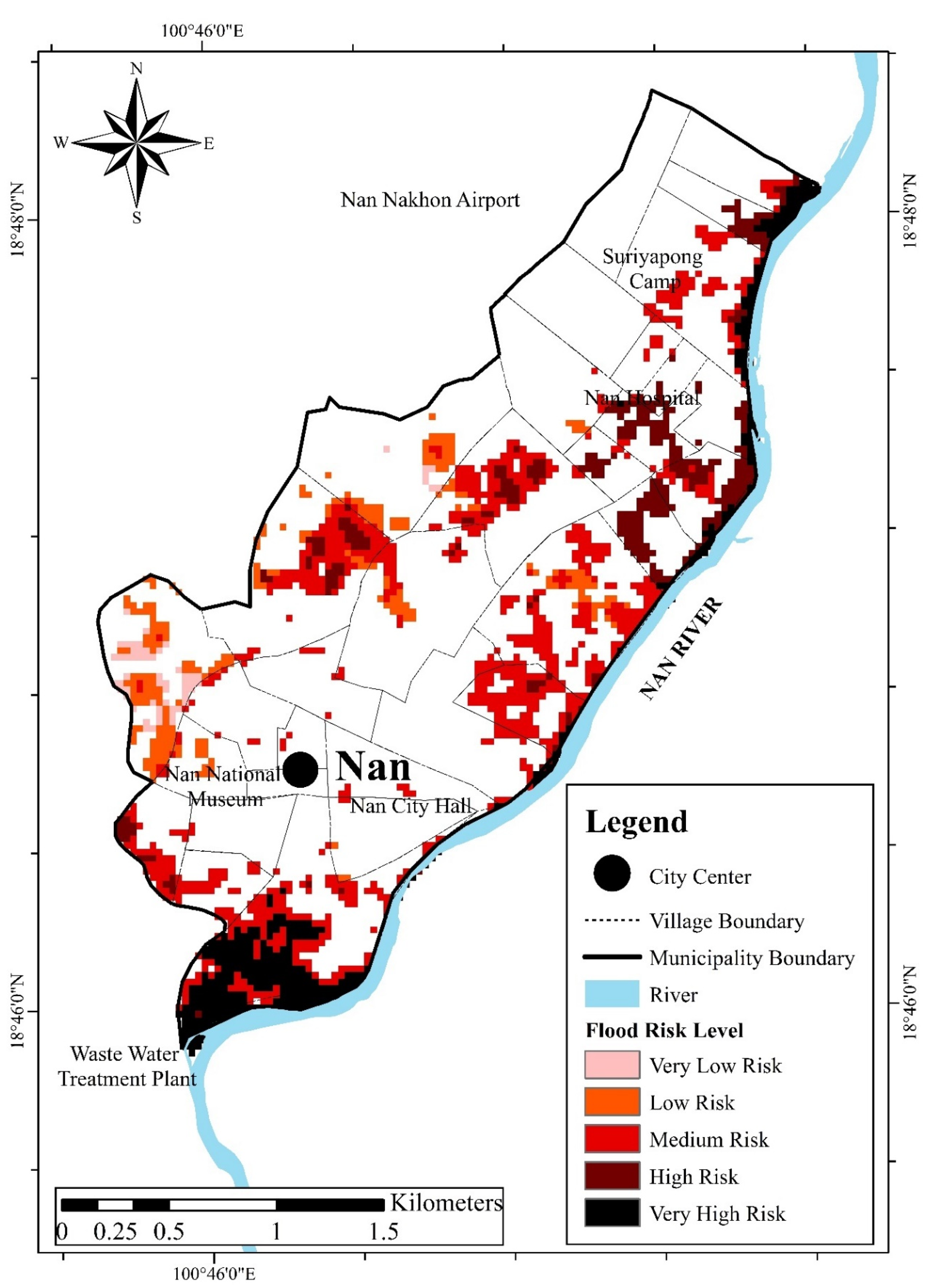
• Flood risks depend on flood hazard probabilities and vulnerabilities. Therefore, flood risks also change with flood probabilities or flood return periods. The study’s results show that when the flood hazard changes, the flood risk also changes correspondingly;
• To mitigate flood problems in the municipal area, various flood control or mitigation measures can be proposed such as dredging of the Nan River channel and its tributaries, raising crest elevations of river flood control levees, or construction of flood bypass channel around the Nan municipal area. The effectiveness of each measure in reducing the flood hazard can be evaluated by using the hydrological model (HEC-HMS) and the hydrodynamic flood routing model (HEC-RAS). Hence, the changes in flood risk in Nan Municipality can be determined. More details can be found in [21].

6. Conclusions

The main results of the present study can be summarized as follows:

• The novelty of this study is the development of an advanced comprehensive and systematic methodology in determining flood hazard, total flood vulnerability, and flood risk at the household level in a municipal area. This is an important improvement over previous studies in which the flood and vulnerability parameters were not all considered. Moreover, these parameters were not systematically determined;
• The methodology was applied to a case study of a municipal area of 7.6 km² in Nan Province, Northern Thailand. The study area was located in the floodplain on the right bank of the Nan River;
• The HEC-HMS hydrological model and the HEC-RAS flood flow simulation model were applied to predict flood depths, velocities, and durations for the return periods of 10, 50, 100, and 500 years;
• The model computed results showed that significant flood hazards occur in Phumin-Thali and Phuang-Payom villages in the southern part of the municipal area and in Mueang Len village in the northeastern part of the area. These villages have low ground elevations, and they are near to Nan River. The central part of the municipal area had less of a flood hazard, as it has a higher ground elevation, and it is far from the river. The computed results were found to be consistent with the past flood situations during the field survey;
• The questionnaire survey in the municipal area reported that the flood duration had the most significant impact on households, while the flood depth and velocity had lesser impacts;
• In-depth analysis of the total vulnerability in the municipal area showed that the vulnerability of the population constituted one-third of the total vulnerability, while the household vulnerability constituted the remaining two-thirds;
• From the computed flood risks, flood risk maps were constructed for various return periods. The maps show that Phumin-Thali and Phuang-Payom villages, located near the right bank of the Nan River, are under very high risk, and more than half of the villages will be inundated and prone to high flood damages. This is consistent with past flood situations;
• The flood risk in the municipal area increased by approximately four times for the increase in the return period from 10 to 500 years;
• Overall, the methodology developed in this study yielded realistic results, and it should be applied to other study areas.

References

1. World Health Organization. Home/Health Topics/Floods. 2021. Available online: https://www.who.int/health-topics/floods (accessed on 7 November 2021).
2. The Organization for Economic Co-operation and Development. Executive summary. In Financial Management of Flood Risk; OECD Publishing: Paris, France, 2016. [Google Scholar] [CrossRef]
3. Ritchie, H.; Roser, M. Natural Disasters. Published Online at OurWorldInData.org. 2014. Available online: https://ourworldindata.org/natural-disasters (accessed on 7 November 2021).
4. Statista. 2021. Available online: https://www.statista.com/statistics/267746/number-of-deaths-globally-due-to-major-flooding/ (accessed on 7 November 2021).
5. Arnell, N.W.; Gosling, S.N. The impacts of climate change on river flood risk at the global scale. Clim. Chang. 2016, 134, 387–401. [Google Scholar] [CrossRef] [Green Version]
6. United Nations Office for Disaster Risk Reduction, UNISDR. Flood Hazard and Risk Assessment; United Nations Office for Disaster Risk Reduction: Geneva, Switzerland, 2017; Available online: https://www.preventionweb.net/files/52828_04floodhazardandriskassessment.pdf (accessed on 15 May 2020).
7. Quesada-Román, A.; Ballesteros-Cánovas, J.A.; Granados-Bolaños, S.; Birkel, C.; Stoffel, M. Dendrogeomorphic reconstruction of floods in a dynamic tropical river. Geomorphology 2020, 359, 107133. [Google Scholar] [CrossRef]
8. Quesada-Román, A.; Villalobos-Chacón, A. Flash flood impacts of Hurricane Otto and hydrometeorological risk mapping in Costa Rica. Geogr. Tidsskr.-Dan. J. Geogr. 2020, 120, 142–155. [Google Scholar] [CrossRef]
9. Tingsanchali, T. Urban flood disaster management. Procedia Eng. 2012, 32, 25–37. [Google Scholar] [CrossRef] [Green Version]
10. Quesada-Román, A.; Ballesteros-Cánovas, J.A.; Granados-Bolaños, S.; Birkel, C.; Stoffel, M. Improving regional flood risk assessment using flood frequency and dendrogeomorphic analyses in mountain catchments impacted by tropical cyclones. Geomorphology 2022, 396, 108000. [Google Scholar] [CrossRef]
11. Kvočka, D.; Falconer, R.A.; Bray, M. Flood hazard assessment for extreme flood events. Nat. Hazards 2016, 84, 1569–1599. [Google Scholar] [CrossRef] [Green Version]
12. Quesada-Román, A.; Castro-Chacón, J.P.; Feoli-Boraschi, S. Geomorphology, land use, and environmental impacts in a densely populated urban catchment of Costa Rica. J. S. Am. Earth Sci. 2021, 112, 103560. [Google Scholar] [CrossRef]
13. García-Soriano, D.; Quesada-Román, A.; Zamorano-Orozco, J.J. Geomorphological hazards susceptibility in high-density urban areas: A case study of Mexico City. J. S. Am. Earth Sci. 2020, 102, 102667. [Google Scholar] [CrossRef]
14. Quesada-Román, A.; Villalobos-Portilla, E.; Campos-Durán, D. Hydrometeorological disasters in urban areas of Costa 13 Rica, Central America. Environ. Hazards 2020, 20, 264–278. [Google Scholar] [CrossRef]
15. Engle, N.L. Adaptive capacity and its assessment. Glob. Environ. Chang. 2011, 21, 647–656. [Google Scholar] [CrossRef]
16. Kron, W. Flood risk = hazard·values·vulnerability. Water Int. 2005, 30, 58–68. [Google Scholar] [CrossRef]
17. Tingsanchali, T.; Karim, F. Flood-hazard assessment and risk-based zoning of a tropical flood plain: Case study of the Yom River, Thailand. Hydrol. Sci. J. 2010, 55, 145–161. [Google Scholar] [CrossRef]
18. Keokhumcheng, Y.; Tingsanchali, T.; Clemente, R.S. Flood risk assessment in the region surrounding the Bangkok Suvarnabhumi Airport. Water Int. 2012, 37, 201–217. [Google Scholar] [CrossRef]
19. Vojtek, M.; Vojteková, J. Flood hazard and flood risk assessment at the local spatial scale: A case study. Geomatics. Nat. Hazards Risk 2016, 7, 1973–1992. [Google Scholar] [CrossRef]
20. Tingsanchali, T.; Keokhumcheng, Y. A method for evaluating flood hazard and flood risk of east Bangkok plain, Thailand. Proc. Inst. Civ. Eng.—Eng. Sustain. 2019, 172, 385–392. [Google Scholar] [CrossRef]
21. Promping, T. Integrated Flood Risk Assessment and Management with Flood Control Measures in Nan Municipality, Thailand. Master’s Thesis, Asian Institute of Technology, Khlong Nueng, Thailand, 2019; 137p. [Google Scholar]
22. Department of Water Resources. Integrated Plans for Water Resources Management in the Nan River Basin; Department of Water Resources: Bangkok, Thailand, 2003. [Google Scholar]
23. Samarasinghe, S.M.J.S.; Nandalal, H.K.; Welivitiya, D.P.; Fowze, J.S.M.; Hazarika, M.K.; Samarakoon, L. Application of Remote Sensing and GIS for Flood Risk Analysis: A Case Study at Kalu- Ganga River, Sri Lanka. In Proceedings of the International Archives of the Photogrammetry, Remote Sensing and Spatial Information Science, Kyoto, Japan, 9–12 August 2010; Volume XXXVIII. Part 8. [Google Scholar]
24. Saaty, T.L. Risk-Its priority and probability: The Analytic Hierarchy Process. Risk Anal. 1987, 7, 159–172. [Google Scholar] [CrossRef]
25. Saaty, T.L. Fundamentals of Decision Making and Priority Theory with the Analytic Hierarchy Process AHP; RWS Publications: Pittsburg, PA, USA, 2000. [Google Scholar]
26. Wangpimool, W.; Pongput, K.; Sukvibool, C.; Sombatpanit, S.; Gassman, P.W. The effect of reforestation on stream flow in Upper Nan river basin using Soil and Water Assessment Tool (SWAT) model. Int. Soil Water Conserv. Res. 2013, 1, 53–63. [Google Scholar] [CrossRef] [Green Version]
27. Department of Disaster Prevention and Mitigation (DDPM). A Development Network of Natural Disasters for Flash Floods and Landslides; Project Final Report; Institute of Science and Technology, Chiang Mai University: Chiang Mai, Thailand, 2010. [Google Scholar]
28. Royal Irrigation Department (RID). Flood Report in the Nan Basin, Thailand [in Thai]; Royal Irrigation Department: Bangkok, Thailand, 2006. [Google Scholar]
29. Poaponsakorn, N.; Meethom, P. Impact of the 2011 Floods, and Flood Management in Thailand; ERIA Discussion Paper Series, ERIA-DP-2013-34; Thailand Development Research Institute, Economic Research Institute for ASEAN and East Asia: Bangkok, Thailand, 2013; Available online: https://www.eria.org/ERIA-DP-2013-34.pdf (accessed on 18 March 2021).
30. Geo-Informatics and Space Technology Development Agency (GISTDA). Radar Satellite Images and Flood Maps of the 2011 Flood; Geo-Informatics and Space Technology Development Agency: Bangkok, Thailand, 2011. [Google Scholar]
31. Seejata, K.; Yodying, A.; Wongthadam, T.; Mahavik, N.; Tantanee, S. Assessment of flood hazard areas using Analytic Hierarchy Process over the Lower Yom Basin, Sukhothai Province. Procedia Eng. 2018, 212, 340–347. [Google Scholar] [CrossRef]
32. Ghosh, A.; Kar, S.K. Application of analytic hierarchy process (AHP) for flood risk assessment: A case study in Malda district of West Bengal, India. Nat. Hazards 2018, 94, 349–368. [Google Scholar] [CrossRef]
33. Alfa, M.I.; Ajibike, M.A.; Daffi, R.E. Application of Analytic Hierarchy Process and Geographic Information System Techniques in Flood Risk Assessment: A Case of Ofu River Catchment in Nigeria. J. Degrad. Min. Lands Manag. 2018, 5, 1363–1372. [Google Scholar] [CrossRef] [Green Version]
34. Intergovernmental Panel on Climate Change, IPCC. Climate Change 2007: Impacts, Adaptation, and Vulnerability. Contribution of Working Group II to the Fourth Assessment Report (Chapter 9); Cambridge University Press: Cambridge, UK, 2007. [Google Scholar]
35. Intergovernmental Panel on Climate Change, IPCC. Climate Change 2007: The physical Science Basis. Contribution of Working Group I to the Fourth Assessment Report (Chapter 11); Cambridge University Press: Cambridge, UK, 2007. [Google Scholar]
36. Hahn, M.B.; Riederer, A.M.; Foster, S.O. The livelihood vulnerability index: A pragmatic approach to assessing risks from climate variability and change—A case study in Mozambique. Glob. Environ. Chang. 2009, 19, 74–88. [Google Scholar] [CrossRef]
37. Yamane, T. Statistics, An Introductory Analysis, 2nd ed.; Harper and Row: New York, NY, USA, 1967. [Google Scholar]
38. U.S. Army Corps of Engineers, USACE. Hydrology Modelling System HEC-HMS, Version 4.2.1; U.S. Army Corps of Engineers: Davis, CA, USA, 2017; Available online: https://www.hec.usace.army.mil/software/hec-hms/documentation/HEC-HMS_ReleaseNotes421.pdf (accessed on 10 December 2018).
39. U.S. Army Corps of Engineers. USACE. HEC-RAS River Analysis System, Version 5.0; U.S. Army Corps of Engineers: Davis, CA, USA, 2016; Available online: https://www.hec.usace.army.mil/software/hec-ras/documentation/HEC-RAS%205.0%20Reference%20Manual.pdf (accessed on 10 December 2018).
40. Chuenchooklin, S.; Taweepong, S.; Pangnakorn, U. Rainfall-runoff Models and Flood Mapping in a Catchment of the Upper Nan Basin. Thailand. J. Water Resour. Hydraul. Eng. 2015, 4, 293–302. [Google Scholar] [CrossRef]
41. Chow, V.T.; Maidment, D.R.; Mays, L.W. Applied Hydrology. 1988. McGraw-Hill. Singapore. Available online: http://ponce.sdsu.edu/Applied_Hydrology_Chow_1988.pdf (accessed on 10 December 2018).
42. Kundzewicz, Z.W.; Kanae, S.; Seneviratne, S.I.; Handmer, J.; Nicholls, N.; Peduzzi, P.; Mechler, R.; Bouwer, L.M.; Arnell, N.; Mach, K.; et al. Flood risk and climate change: Global and regional perspectives. Hydrol. Sci. J. 2014, 59, 1–28. [Google Scholar] [CrossRef] [Green Version]
Figure 1. Number of deaths due to the fact of floods worldwide from 1900 to 2020 [3].
Water 14 00161 g001
Figure 2. Upstream sub-basins of the Nan River for hydrologic modeling (HEC-HMS).
Water 14 00161 g002
Figure 3. Nan River near Nan Province and its municipality area for hydrodynamic modeling (HEC-RAS).
Water 14 00161 g003
Figure 4. Methodology and computational procedure for calculation of the flood hazard, flood damage vulnerability, and flood risk at the household level in the municipal study area.
Water 14 00161 g004
Figure 5. Configuration of the HEC-HMS and HEC-RAS models for the upstream sub-basins of the Nan River and the Nan municipal area.
Water 14 00161 g005
Figure 6. Results of the HEC-HMS model’s calibration from 2006 to 2011 and verification from 2012 to 2017 at Tha Wang Pha station (N64) and Mueang Nan station (N1).
Water 14 00161 g006
Figure 7. Results of the HEC-RAS model’s calibration of flood events in 2006 and 2011 and its verification in 2013 and 2016 at Mueang Nan station (N1), Nan River.
Water 14 00161 g007
Figure 8. Flood hazard map for 100 year return period in the Nan municipal area.
Water 14 00161 g008
Figure 9. Flood hazard map for 500 year return period in the Nan municipal area.
Water 14 00161 g009
Figure 10. Vulnerability map of Nan Municipality.
Water 14 00161 g010
Figure 11. Flood risk map of the 100 year return period in the Nan Municipality.
Water 14 00161 g011
Figure 12. Flood risk maps of the 500 year return period in the Nan Municipality.
Water 14 00161 g012