Dynamic Changes in Groundwater Level under Climate Changes in the Gnangara Region, Western Australia

Abstract

The groundwater-dependent ecosystem in the Gnangara region is confronted with great threats due to the decline in groundwater level since the 1970s. The aim of this study is to apply multiple trend analysis methods at 351 monitoring bores to detect the trends in groundwater level using spatial, temporal and Hydrograph Analysis: Rainfall and Time Trend models, which were applied to evaluate the impacts of rainfall on the groundwater level in the Gnangara region, Western Australia. In the period of 1977–2017, the groundwater level decreased from the Gnangara’s edge to the central-north area, with a maximum trend magnitude of −0.28 m/year. The groundwater level in 1998–2017 exhibited an increasing trend in December–March and a decreasing trend in April–November with the exception of September when compared to 1978–1997. The rainfall + time model based on the cumulative annual residual rainfall technique with a one-month lag during 1990–2017 was determined as the best model. Rainfall had great impacts on the groundwater level in central Gnangara, with the highest impact coefficient being 0.00473, and the impacts reduced gradually from the central area to the boundary region. Other factors such as pine plantation, the topography and landforms, the Tamala Limestone formation, and aquifer groundwater abstraction also had important influences on the groundwater level.

1. Introduction

Groundwater is the world’s third largest reservoir of water resources and the largest reservoir of liquid fresh water on Earth. It is also an important natural resource for human survival and it provides drinking water to more than 2 billion people around the world [1,2]. It is of great significance for maintaining the sustainability of rivers, wetlands, lakes and aquatic communities [3,4,5,6]. Groundwater level is a stable and observable groundwater variable in the basin, and the important hydrological processes and the driving factors of groundwater dynamics can be identified by analyzing groundwater level [7]. Simultaneously, changes in groundwater level are important indicators reflecting the condition of groundwater resources in a region. Research on the dynamic changes of groundwater level is of great importance for studying the hydrological water cycle, water resource evolution, water balance and the sustainability of social and economic development. However, dynamic changes in groundwater level are complicated, hydrologically changing processes and are influenced by the combination of climate change and human activity. Groundwater resources are faced with the challenges of water supply and sustainability all over the world [8,9,10]. Climate changes have aggravated the unbalanced distribution of water resources and changed the groundwater cycle. Since 1960, the demand for groundwater is increasing due to urban expansion, population growth and industrial and agricultural development [6,8,11]. Additionally, the long-term over-exploitation of groundwater has resulted in a decline in groundwater level and shortages of groundwater resources, which in turn triggers social conflicts, limits economic development, and breaks the balance of ecosystems that depend on groundwater level [6,8,12,13,14,15].

Groundwater level varies over time and space, and it is influenced by a variety of factors such as climate, hydrology, geology, human activities and sunspots. For studying the dynamic changes in groundwater level, it is necessary to examine and analyze the changes in groundwater level in time and space on the basis of the collected groundwater level observations. Research on the temporal characteristics of groundwater level variation is generally based on mathematical statistics and time series analysis methods, whereas research on the spatial variation of groundwater level generally utilizes geostatistical analysis methods. Groundwater level trend analysis methods have been greatly developed in recent years, from simple linear regression to more complex parametric and non-parametric tests [16,17]. Parametric methods are generally based on linear models and residual models, which are more effective than non-parametric methods; however, parametric methods require data to be independent and normally distributed, and require t-tests to test the significance of the slope of the regression model, which may be inaccurate for time series data with seasonal characteristics [18,19,20]. The most commonly used nonparametric methods for testing trends in hydrologic time series are the Mann-–Kendall (MK) test and Sen’s slope estimator [21,22,23,24,25]. The MK test is a robust nonparametric test to quantify the significance of trends in data with seasonal variability and missing values. This test was further improved by taking into account a seasonality by Hirsch et al. (1982) [26]. Sen’s slope estimator is a nonparametric test proposed by Sen (1968) [24]. It is the unbiased estimation of linear trends and magnitudes. The accuracy is high in highly skewed data compared to regression estimators [24,27]. In recent years, nonparametric tests have been widely used to detect trends in precipitation and temperature, evaporation, runoff, groundwater dynamics, and water quality [23,28,29,30,31,32,33,34]. The innovative trend analysis developed by Şen (2012) is a new approach to test a time series trend [35]. This method does not require restrictive assumptions such as the independent structure of the time series, the normality of the distribution, and length of data, which are required for classical techniques, such as MK and Spearman’s rho (SR) tests [36].

Dynamic changes in groundwater levels are influenced by a combination of factors which can generally be divided into natural and human factors. Natural factors include climate change, changes in hydrogeological conditions, changes in river levels, geological activities, changes in the physical and chemical properties of soil, biological activities, earthquakes and bush fires. Human factors include groundwater extraction, changes in land use and land cover, water conservancy facilities, and agricultural irrigation. In most regions, changes in the groundwater level are mainly influenced by climate change. Recharge reductions induced by climate change have a greater impact on global groundwater depletion than groundwater pumping [37]. Climate change (rainfall, evaporation and temperature) leads to changes in the water cycle and the groundwater storage and recharge conditions, which results in changes in groundwater level. The rainfall amount and rainfall distribution in time and space have significant impacts on groundwater level changes [38]. A data-based method called the Hydrograph Analysis: Rainfall and Time Trends (HARTT) was developed by Ferdowsian et al. (2001) [39] and Ferdowsian et al. (2002) [40], and is widely used to calculate rainfall’s impacts on groundwater level. This model requires that the groundwater level observations have no missing value and are continuous in time.

Groundwater is the most important water resource in southwest Australia and is mainly used for domestic water, mines, gardens, parks, and industry. With the rapid development of the economy and the increase in population, the total water consumption has increased sharply. A total of 75% of the water consumption in this area comes from groundwater [41]. Due to the continuous growth of the mining industry, the population of Perth City is growing at a rate of 22,500 people per year (1.4%) [42]. The Gnangara groundwater system is the main source of drinking water in Perth City, providing approximately 165 GL of domestic and commercial water for residents every year, equivalent to 65% of the water consumption of the whole city. In 1975, 16% of drinking water came from groundwater, but with the decrease in runoff, this proportion increased since 2002 to more than 60% [43]. From the late 1980s to the late 1990s, groundwater storage decreased at the rate of 20 GL per year in the north and central area of the Gnangara region due to the continuous drought of the climate, and the public and private extraction of groundwater [43]. Since the late 1990s, groundwater storage has decreased at a rate of 45 GL per year and the groundwater level in some areas has decreased to 5 m [43]. In the last 40 years, groundwater levels in both the unconfined and confined aquifers in the Gnangara region have shown a decline, and the Gnangara groundwater system and its supporting ecosystems are under great threat in the current context of climate change. Therefore, the main objective of this study is to (1) investigate the temporal and spatial variation trend in the groundwater level in an unconfined aquifer of the Gnangara region by using multiple trend analysis methods, (2) provide an overview of the factors influencing the groundwater level, and (3) quantitatively estimate the impact of rainfall on the dynamic changes in groundwater level and the lag time between rainfall and its impact on groundwater level by the HARTT model. The research provides new insight for the spatiotemporal dynamics of the groundwater levels and are helpful for planners and policy makers for the sustainable management of groundwater resources.

2. Materials and Methods

2.1. Site Location

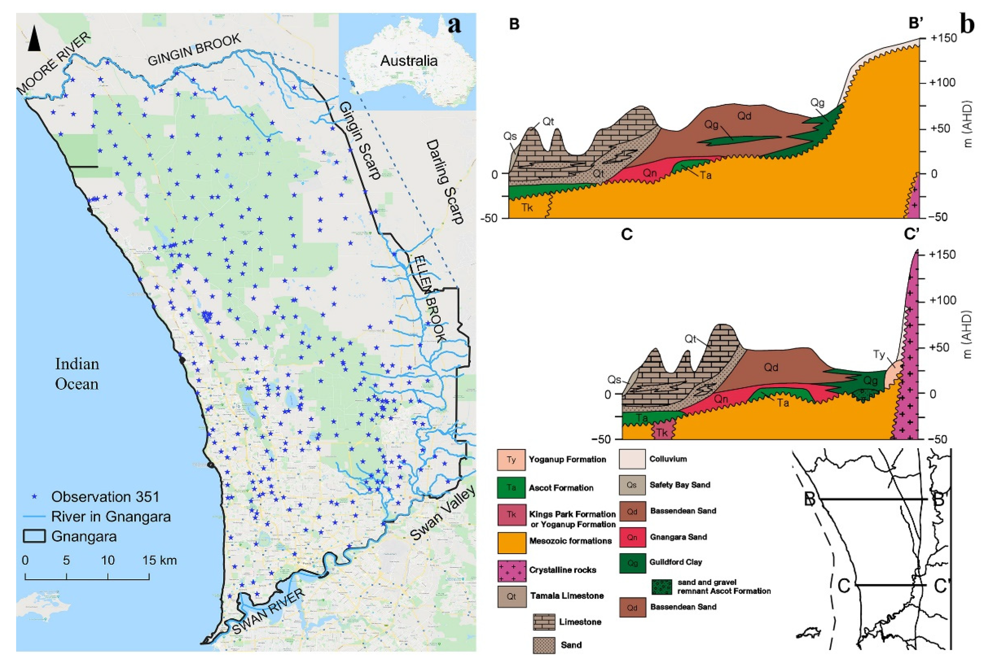
The Gnangara region is located at approximately −31.29° S~−32.05° S and 115.50° E–116.07° E in the southwestern area of Western Australia (Figure 1). Under the Mediterranean climate of the Gnangara region, the average annual rainfall is 758 mm, and 80% of the rainfall is concentrated in May to September when groundwater is recharged [44]. Rainfall is the main recharge source of groundwater in the Gnangara region. However, the rainfall is detected as being in decline in the recent 40 years. Rainfall during the period of 1968–2017 was reduced by 13% compared with rainfall during the period of 1900–2017 [44]. The groundwater system in this region is out of balance due to a faster reduction in rainfall than groundwater exploitation. Since the 1970s, the groundwater level in this region has shown a decline because of the high groundwater use and lower rainfall [45].

There are four main aquifers in the Gnagara region including the Superficial aquifer, Mirrabooka aquifer, Leederville aquifer and Yarragadee aquifer (A 3D aquifer map can be accessed at website of http://www.bom.gov.au/water/groundwater/explorer/3d-aquifer-visual.shtml (accessed on 7 January 2021)). The Superfical aquifer is a major unconfined aquifer which stretches across the entire Gnangara region with a mean thickness of 50 m and a maximum thickness of 70 m and it comprises the quaternary–tertiary sediments of the Swan Coastal Plain (Figure 1b) [46]. From the eastern inland to the western coast, the sediments of the Superficial aquifer vary from Guildford Clay in the east, Bassendean sand and Gnangara Sand in the center, to Tamala Limestone and Safety Bay Sand in the west (Figure 1b) [47]. The groundwater recharge in the Superficial aquifer is determined by the local rainfall, land use and hydrogeological conditions [46,48]. The main recharge source of the groundwater in the Gnangara region is winter rainfall. Other sources come from the upward recharge from the underlying Leederville and Yarragadee aquifers [48]. The groundwater level in the Gnangara region varies in depth. The groundwater level mainly flows from the east to the western coast in the northern Gnangara region and flows to the central-east area of the southern Gnangara region [46,49]. The hydraulic properties of the Superficial aquifer vary significantly depending on geology. For the Guildford Clay in the eastern Gnangara region (Figure 1b), which consists of clayey sediments, basal sandy lenses, Safety Bay Sand, and Becher Sand, the hydraulic conductivities vary between 0.1 m/day and 15 m/day [46]. The Bassendean and Gnangara sands (Figure 1b) are characterized by permeability with average horizontal hydraulic conductivities of 15 m/day and 20 m/day, respectively [46]. The Tamala Limestone in the western Gnangara region (Figure 1b) contains numerous solution channels and cavities and the horizontal hydraulic conductivities range between 100 and 1000 m/day [46].

2.2. Data Sources

In this study, the rainfall and groundwater level time series data of 351 groundwater level observation bores from 1977 to 2017 were used. Rainfall data were derived from the SILO Data Drill database and this dataset can be downloaded from website https://www.longpaddock.qld.gov.au/silo/ (accessed on 7 January 2021). Groundwater level observation bores are distributed in the Superficial aquifer and the data are irregularly recorded and can be acquired from the website https://water.wa.gov.au/maps-and-data/monitoring/water-information-reporting (accessed on 7 January 2021). The groundwater level data were included in a monthly dataset and were measured from logged bores in the Australian Height Datum (AHD) using meters as the unit of measurement. The detailed information, including the start of the records, the date of the well construction, and the depths of the monitoring wells, was described in Appendix A,

Table A1. Instructions of the groundwater level monitoring wells.

Bore ID	Start Date of Record	Longitude	Latitude	Date of Well Construction	Well Depth (m)
bore61610005	1978-06	115.761	−31.993	1978-06	23
bore61610006	1978-06	115.763	−31.917	1978-06	21
bore61610007	1953-05	115.759	−31.866	1953-05	0
bore61610012	1967-10	115.759	−31.850	1967-10	0
bore61610013	1974-09	115.758	−31.833	1974-09	51
bore61610015	1946-10	115.777	−31.979		0
bore61610016	1978-06	115.768	−31.955	1978-06	26
bore61610020	1970-07	115.797	−31.990	1970-07	3.9
bore61610021	1978-06	115.792	−31.975	1978-06	30
bore61610029	1978-06	115.795	−31.926	1978-06	17
bore61610031	1974-07	115.794	−31.892	1974-07	18.3
bore61610032	1972-03	115.796	−31.886	1972-03	0
bore61610033	1974-07	115.790	−31.883	1974-07	23.9
bore61610036	1974-07	115.789	−31.871	1974-07	21.4
bore61610037	1974-07	115.799	−31.864	1974-07	17.1
bore61610038	1974-07	115.793	−31.855	1974-07	20.9
bore61610039	1974-07	115.791	−31.846	1974-07	16.2
bore61610040	1967-09	115.786	−31.834	1967-09	0
bore61610045	1978-06	115.815	−31.963	1978-06	21
bore61610050	1974-07	115.810	−31.900	1974-07	21.8
bore61610100	1974-07	115.815	−31.859	1974-07	16
bore61610106	1974-07	115.802	−31.845	1974-07	24.7
bore61610107	1974-07	115.815	−31.851	1974-07	28.4
bore61610110	1974-07	115.811	−31.842	1972-04	35.6
bore61610111	1971-06	115.805	−31.829	1972-06	0
bore61610112	1965-09	115.815	−31.818		0
bore61610142	1974-07	115.821	−31.869	1974-07	19.8
bore61610143	1974-07	115.830	−31.866	1974-07	24.5
bore61610161	1978-06	115.844	−31.939	1978-06	15.8
bore61610163	1974-07	115.838	−31.882	1974-07	37.1
bore61610171	1978-06	115.859	−31.908	1978-05	15
bore61610172	1974-01	115.852	−31.875	1974-01	62.2
bore61610200	1946-08	115.879	−31.911	1946-08	7
bore61610204	1947-11	115.876	−31.891	1947-11	8
bore61610277	1969-04	115.897	−31.898	1969-04	0
bore61610283	1981-12	115.899	−31.874		0
bore61610284	1952-10	115.892	−31.872		0
bore61610381	1922-03	115.915	−31.928	1922-03	0
bore61610474	1947-08	115.923	−31.889		0
bore61610475	1974-01	115.919	−31.872	1974-01	12.8
bore61610493	1977-07	115.932	−31.820	1977-07	18
bore61610510	1974-01	115.941	−31.856	1974-01	13.2
bore61610511	1977-01	115.951	−31.856	1900-01	4
bore61610513	1976-02	115.937	−31.846	1975-06	48
bore61610517	1976-06	115.951	−31.846	1976-06	5
bore61610522	1976-05	115.943	−31.838	1976-05	6
bore61610525	1977-03	115.952	−31.832	1977-06	15
bore61610543	1978-06	115.958	−31.900	1978-05	17.5
bore61610546	1977-01	115.966	−31.856	1977-01	5
bore61610550	1976-05	115.957	−31.846	1976-05	6
bore61610559	1977-03	115.961	−31.820	1977-03	17
bore61610561	1977-08	115.969	−31.820	1977-06	15
bore61610563	1974-06	115.959	−31.813	1974-06	14
bore61610570	1977-01	115.978	−31.851	1977-01	6
bore61610572	1977-10	115.981	−31.840	1977-10	12
bore61610575	1977-02	115.979	−31.827	1977-06	14
bore61610576	1977-01	115.985	−31.819	1977-06	17
bore61610577	1976-04	115.979	−31.813	1976-06	25
bore61610582	1975-08	115.669	−31.558	1975-08	16.8
bore61610584	1974-12	115.709	−31.624	1974-06	56
bore61610585	1974-12	115.716	−31.602	1974-06	58
bore61610586	1974-12	115.718	−31.572	1974-06	52
bore61610587	1976-10	115.707	−31.556	1976-10	37.8
bore61610591	1973-06	115.720	−31.732	1973-06	43
bore61610594	1976-10	115.731	−31.587	1976-10	46
bore61610595	1977-01	115.735	−31.553	1977-01	73
bore61610596	1974-08	115.740	−31.778	1974-08	39
bore61610599	1974-12	115.738	−31.692	1974-06	59
bore61610600	1976-12	115.752	−31.660	1976-12	32.1
bore61610601	1976-11	115.747	−31.642	1976-11	43.4
bore61610603	1976-10	115.739	−31.608	1976-10	45.7
bore61610608	1978-10	115.751	−31.517	1978-05	62
bore61610613	1976-11	115.762	−31.626	1976-11	45.9
bore61610615	1975-06	115.761	−31.605	1975-05	75
bore61610617	1975-06	115.762	−31.587	1975-05	82
bore61610619	1975-06	115.760	−31.570	1975-06	83
bore61610620	1975-07	115.757	−31.561	1975-06	84
bore61610622	1976-10	115.764	−31.551	1976-10	41.3
bore61610624	1978-10	115.755	−31.534	1978-05	72
bore61610627	1972-03	115.782	−31.777	1972-06	0
bore61610628	1981-09	115.784	−31.726	1981-09	0
bore61610632	1974-08	115.779	−31.688	1974-08	70
bore61610633	1976-12	115.771	−31.669	1976-12	44.9
bore61610642	1981-02	115.771	−31.636	1973-06	68
bore61610644	1976-10	115.778	−31.578	1976-10	31.5
bore61610645	1976-10	115.781	−31.566	1976-10	33
bore61610649	1982-05	115.781	−31.538	1982-05	48
bore61610652	1982-05	115.781	−31.538	1982-05	48
bore61610654	1977-07	115.777	−31.505	1977-06	31
bore61610661	1970-06	115.796	−31.745	1970-06	0
bore61610662	1975-02	115.788	−31.725	1975-02	20.7
bore61610664	1975-03	115.797	−31.705	1975-03	40
bore61610665	1975-02	115.795	−31.687	1975-02	39.6
bore61610667	1975-04	115.793	−31.653	1975-04	74
bore61610670	1986-04	115.792	−31.610		0
bore61610671	1976-10	115.794	−31.594	1976-10	25.9
bore61610672	1976-10	115.802	−31.573	1976-10	30.8
bore61610673	1976-11	115.801	−31.547	1976-11	36.1
bore61610674	1978-11	115.802	−31.526	1978-08	68
bore61610676	1978-11	115.799	−31.508	1978-10	66
bore61610677	1972-10	115.809	−31.806	1972-06	0
bore61610678	1972-03	115.814	−31.784	1900-01	68.6
bore61610679	1978-11	115.803	−31.788	1978-02	13.5
bore61610683	1975-02	115.808	−31.751	1975-02	41.4
bore61610684	1975-02	115.811	−31.734	1900-01	27.4
bore61610685	1979-01	115.811	−31.728	1979-01	9
bore61610688	1978-12	115.810	−31.722	1978-12	9
bore61610690	1972-06	115.806	−31.714	1972-06	58.5
bore61610696	1965-08	115.808	−31.673	1965-08	48.5
bore61610697	1977-02	115.810	−31.649	1977-02	14
bore61610698	1976-12	115.819	−31.628	1976-12	13.2
bore61610712	1973-09	115.808	−31.479	1973-06	62.4
bore61610714	1973-09	115.832	−31.805	1973-09	31.7
bore61610715	1963-08	115.833	−31.796	1963-08	72.3
bore61610716	1975-02	115.827	−31.771	1975-02	53.6
bore61610720	1981-03	115.832	−31.756	1973-06	93.2
bore61610734	1979-05	115.823	−31.733	1979-12	16
bore61610736	1978-12	115.823	−31.725	1978-12	9
bore61610745	1979-05	115.836	−31.725	1979-02	13
bore61610750	1976-10	115.829	−31.658	1976-10	13.5
bore61610753	1965-10	115.830	−31.635	1965-10	38.1
bore61610756	1976-12	115.832	−31.587	1976-12	20.8
bore61610758	1975-08	115.852	−31.782	1975-08	32.9
bore61610761	1977-09	115.837	−31.755	1977-09	30
bore61610762	1977-09	115.852	−31.752	1977-09	10.7
bore61610764	1977-04	115.851	−31.749	1977-03	27
bore61610769	1977-04	115.852	−31.729	1977-03	30
bore61610789	1965-06	115.836	−31.708	1965-05	40.5
bore61610794	1975-02	115.853	−31.686	1975-02	16
bore61610803	1976-11	115.846	−31.634	1976-11	13.4
bore61610804	1976-11	115.843	−31.612	1976-11	17.1
bore61610805	1976-11	115.845	−31.573	1976-11	19.5
bore61610807	1971-03	115.845	−31.543	1971-03	81.7
bore61610808	1976-11	115.843	−31.529	1976-11	29.1
bore61610809	1977-07	115.840	−31.507	1977-07	26
bore61610810	1977-07	115.844	−31.478	1977-06	32
bore61610811	1974-06	115.854	−31.805	1974-06	22.4
bore61610815	1981-12	115.862	−31.795	1900-01	21.1
bore61610816	1963-09	115.866	−31.765	1963-09	48.8
bore61610817	1975-02	115.853	−31.746	1975-02	17.7
bore61610822	1977-04	115.853	−31.738	1977-04	20
bore61610832	1975-02	115.863	−31.672	1975-02	13.1
bore61610833	1975-02	115.855	−31.655	1975-02	14.4
bore61610834	1976-12	115.861	−31.597	1976-12	19.1
bore61610835	1973-09	115.875	−31.804	1973-09	16.5
bore61610843	1973-09	115.876	−31.785	1973-09	25.6
bore61610845	1975-02	115.881	−31.752	1975-02	8.2
bore61610855	1981-10	115.878	−31.716	1981-05	19.8
bore61610860	1975-02	115.879	−31.692	1975-02	13.5
bore61610861	1965-09	115.876	−31.661	1965-09	32
bore61610864	1976-11	115.881	−31.631	1976-11	17.2
bore61610869	1976-11	115.877	−31.522	1976-11	23.1
bore61610870	1977-08	115.877	−31.510	1977-08	24.5
bore61610871	1973-09	115.878	−31.483	1973-07	57
bore61610883	1973-09	115.898	−31.786	1973-09	15.8
bore61610884	1963-07	115.895	−31.768	1963-07	33.5
bore61610907	1983-05	115.894	−31.683	1983-05	11
bore61610908	1975-02	115.895	−31.662	1975-02	14.9
bore61610913	1983-03	115.895	−31.618	1983-03	13.5
bore61610914	1977-01	115.896	−31.598	1977-01	21.2
bore61610915	1971-03	115.891	−31.571	1971-03	78.9
bore61610917	1977-07	115.905	−31.477	1977-07	13.7
bore61610918	1974-01	115.918	−31.804	1974-01	13.4
bore61610933	1963-10	115.927	−31.771	1963-10	39.6
bore61610936	1983-05	115.910	−31.701	1983-05	17.5
bore61610941	1983-06	115.907	−31.694	1983-06	19
bore61610943	1975-02	115.907	−31.692	1975-02	16.1
bore61610946	1982-11	115.905	−31.676	1982-11	11
bore61610949	1983-05	115.917	−31.667	1983-05	8.8
bore61610951	1973-06	115.916	−31.539	1973-06	23
bore61610952	1977-08	115.910	−31.507	1977-08	17
bore61610953	1977-06	115.909	−31.455	1977-06	14
bore61610967	1984-01	115.930	−31.759	1900-01	10
bore61610978	1975-03	115.922	−31.728	1975-03	16.7
bore61610980	1984-01	115.929	−31.720	1900-01	10
bore61610982	1982-11	115.934	−31.714	1982-11	8.3
bore61610983	1975-02	115.930	−31.694	1975-02	16.5
bore61610984	1983-05	115.933	−31.682	1983-05	11
bore61610985	1977-07	115.935	−31.473	1977-07	3
bore61610989	1973-09	115.939	−31.785	1973-09	15.8
bore61611003	1981-04	115.950	−31.791	1976-06	8
bore61611010	1984-01	115.950	−31.759	1900-01	10
bore61611011	1984-01	115.940	−31.740	1900-01	13
bore61611014	1984-01	115.951	−31.740	1900-01	23
bore61611018	1984-01	115.948	−31.722	1900-01	10
bore61611019	1965-08	115.950	−31.674	1900-01	31.1
bore61611021	1983-03	115.941	−31.647	1983-03	15
bore61611022	1977-07	115.943	−31.500	1977-07	13
bore61611023	1978-06	115.949	−31.499	1978-06	16
bore61611025	1978-08	115.954	−31.804	1978-08	16
bore61611031	1973-10	115.957	−31.762	1971-06	47
bore61611033	1984-01	115.968	−31.764	1900-01	14
bore61611034	1971-06	115.957	−31.752	1971-06	19.7
bore61611035	1976-04	115.957	−31.742	1971-06	157
bore61611037	1984-01	115.961	−31.742	1900-01	9
bore61611041	1984-01	115.969	−31.721	1900-01	10
bore61611042	1983-05	115.957	−31.696	1983-05	9
bore61611043	1965-10	115.968	−31.641	1965-09	25.1
bore61611044	1970-02	115.959	−31.586	1970-02	85.3
bore61611047	1978-06	115.972	−31.553	1978-06	15
bore61611056	1984-01	115.972	−31.742	1900-01	10
bore61611064	1984-01	115.999	−31.770	1900-01	12
bore61611065	1984-01	115.994	−31.742	1900-01	6
bore61611068	1984-01	115.992	−31.718	1900-01	8
bore61611072	1978-06	116.006	−31.670	1978-06	15
bore61611074	1978-06	116.009	−31.805	1978-05	17
bore61611076	1984-01	116.009	−31.772	1900-01	12
bore61611079	1984-01	116.005	−31.742	1900-01	8
bore61611082	1984-01	116.015	−31.716	1900-01	8
bore61611083	1978-06	116.016	−31.642	1978-06	18
bore61611087	1977-07	115.872	−31.448	1977-06	16
bore61611088	1977-12	115.898	−31.435	1977-12	13.6
bore61611089	1977-07	115.916	−31.420	1977-07	13
bore61611092	1974-12	115.650	−31.584	1974-06	40.9
bore61611151	1989-01	115.822	−31.621		0
bore61611175	1984-12	115.970	−31.696	1900-01	8
bore61611183	1984-01	115.992	−31.699	1900-01	7
bore61611211	1985-11	115.804	−31.861	1985-01	18
bore61611220	1989-12	115.734	−31.631	1989-03	4.3
bore61611223	1989-12	115.731	−31.629	1989-03	13.4
bore61611225	1989-11	115.728	−31.629	1989-03	7.65
bore61611228	1990-01	115.736	−31.635	1989-03	8.4
bore61611233	1989-12	115.733	−31.639	1989-03	8.4
bore61611234	1989-11	115.731	−31.637	1989-03	13.4
bore61611240	1989-12	115.737	−31.630	1989-03	10.4
bore61611244	1989-12	115.735	−31.631	1989-03	26
bore61611247	1990-01	115.729	−31.633	1989-03	7.2
bore61611270	2001-10	115.902	−31.914	2001-07	7
bore61611289	2001-12	115.869	−31.711	2001-09	11.8
bore61611303	1990-02	115.708	−31.588	1990-01	6.6
bore61611377	2012-05	115.863	−31.790	2011-12	7
bore61611652	1989-08	115.716	−31.693	1989-08	61.5
bore61611656	1989-08	115.720	−31.702	1989-08	71
bore61611663	1989-11	115.722	−31.715	1989-08	59.5
bore61611664	1989-08	115.725	−31.669	1989-08	48
bore61611666	1989-08	115.697	−31.677	1989-08	45
bore61611667	1989-06	115.686	−31.615	1989-06	62.4
bore61611668	1989-06	115.698	−31.615	1989-06	68
bore61611669	1989-06	115.664	−31.621	1989-06	20
bore61611670	1989-06	115.657	−31.605	1989-06	26.5
bore61611673	1989-07	115.688	−31.599	1989-07	68.5
bore61611674	1989-07	115.700	−31.631	1989-07	63.5
bore61611676	1989-08	115.675	−31.634	1989-08	26
bore61611677	1989-08	115.683	−31.631	1989-08	51
bore61611678	1989-08	115.713	−31.654	1989-08	57
bore61611680	1989-08	115.706	−31.645	1989-08	44.5
bore61611681	1989-09	115.683	−31.647	1989-09	29.5
bore61611682	1989-09	115.689	−31.622	1989-09	73.5
bore61611685	1989-09	115.668	−31.596	1989-09	55
bore61611702	1990-07	115.698	−31.682	1990-06	8.85
bore61611833	1996-06	115.760	−32.003	1996-06	26
bore61611941	1993-05	115.846	−31.612	1993-05	8.72
bore61611960	2010-09	115.807	−31.945	2008-01	15
bore61611974	2010-09	115.770	−31.976	2008-03	28.6
bore61611975	2010-09	115.768	−31.906	2008-03	15
bore61611976	2010-09	115.744	−31.818	2008-03	17.6
bore61611977	2010-09	115.759	−31.886	2008-03	30.7
bore61612100	1991-05	115.712	−31.537	1991-05	61.3
bore61612101	1991-05	115.703	−31.539	1991-05	45
bore61612102	1991-06	115.692	−31.541	1991-05	33.1
bore61612103	1991-05	115.689	−31.542	1991-05	10.7
bore61612104	1991-05	115.685	−31.543	1991-05	8.96
bore61612105	1991-05	115.697	−31.555	1991-05	21.5
bore61612106	1991-05	115.687	−31.555	1991-05	15.2
bore61612107	1991-05	115.696	−31.570	1991-05	17.9
bore61613200	1995-09	115.944	−31.766	1995-08	9.55
bore61613201	1995-11	115.957	−31.750	1995-08	10
bore61613202	1995-09	115.947	−31.736	1995-08	9.97
bore61613203	1995-09	115.827	−31.687	1995-08	8.41
bore61613204	1995-11	115.840	−31.653	1995-08	12
bore61613205	1995-10	115.819	−31.611	1995-08	11.7
bore61613206	1995-10	115.815	−31.604	1995-08	13.1
bore61613208	1995-09	115.699	−31.568	1995-08	14.7
bore61613209	1995-10	115.697	−31.568	1995-08	14.1
bore61613210	1995-10	115.718	−31.508	1995-08	11.7
bore61613211	1995-09	115.854	−31.667	1995-08	12.8
bore61613213	1995-09	115.964	−31.704	1995-08	8.13
bore61613214	1995-09	115.963	−31.743	1995-09	2.91
bore61613215	1995-09	115.959	−31.752	1995-09	2.4
bore61613217	1994-01	115.974	−31.753	1995-10	0
bore61613231	1999-02	115.915	−31.705	1999-02	10.1
bore61618432	1995-07	115.805	−31.762	1995-04	19
bore61618440	1996-06	115.874	−31.790	1996-06	5.67
bore61618441	1996-07	115.861	−31.821	1996-06	25.4
bore61618444	1997-07	115.962	−31.836	1997-06	7.95
bore61618499	1997-08	115.763	−31.721	1996-11	70
bore61618500	1997-03	115.690	−31.575	1997-02	6.54
bore61618513	1997-10	115.764	−31.866	1997-09	13
bore61618558	1998-10	115.975	−31.662	1998-06	6.3
bore61618559	1998-07	116.013	−31.606	1998-06	18
bore61618606	2000-03	115.995	−31.795		0
bore61618607	2000-03	115.980	−31.771		0
bore61619294	1988-09	116.041	−31.845	1987-02	20.4
bore61619296	1988-09	116.037	−31.822	1987-02	12
bore61619406	1990-08	115.591	−31.482	1990-07	66
bore61619455	1990-08	115.589	−31.482	1979-05	61
bore61619461	1985-07	115.581	−31.484	1973-03	15
bore61619464	1980-06	115.586	−31.483	1980-06	55
bore61619608	1985-07	116.007	−31.830	1985-07	12
bore61619611	1985-07	116.025	−31.813	1985-07	17
bore61619615	1985-07	115.978	−31.873	1985-07	19
bore61620100	1992-05	115.737	−31.750	1992-05	53.7
bore61620101	1992-05	115.735	−31.785	1992-05	41.8
bore61620102	1992-05	115.742	−31.795	1992-05	48.3
bore61620103	1992-05	115.750	−31.807	1992-05	36.2
bore61620104	1992-05	115.758	−31.815	1992-05	59.7
bore61620110	1992-05	115.772	−31.784	1992-05	50.8
bore61620111	1992-05	115.768	−31.803	1992-05	58.6
bore61620112	1992-05	115.733	−31.753	1992-05	75.4
bore61625172	1995-06	115.723	−31.708	1994-08	42.1
bore61710001	1978-06	115.535	−31.372	1978-06	43.9
bore61710002	1978-06	115.545	−31.399	1978-06	46
bore61710003	1974-12	115.551	−31.350	1974-12	38.4
bore61710006	1977-07	115.561	−31.374	1977-07	37.6
bore61710007	1978-05	115.560	−31.329	1978-05	36
bore61710008	1977-07	115.586	−31.389	1977-05	55
bore61710010	1978-05	115.586	−31.349	1978-05	46
bore61710011	1977-07	115.595	−31.420	1977-04	63
bore61710013	1977-08	115.596	−31.329	1977-08	64.5
bore61710014	1973-06	115.605	−31.307	1973-06	38.3
bore61710017	1978-07	115.620	−31.373	1978-07	42
bore61710018	1973-06	115.620	−31.362	1973-06	80.9
bore61710022	1977-07	115.653	−31.375	1977-06	35
bore61710023	1977-07	115.654	−31.354	1977-04	15
bore61710025	1974-04	115.665	−31.545	1974-04	0
bore61710026	1974-04	115.655	−31.509	1974-04	0
bore61710027	1977-07	115.655	−31.479	1977-05	45
bore61710028	1974-04	115.677	−31.544		0
bore61710031	1974-01	115.684	−31.476	1973-06	66.2
bore61710033	1977-07	115.685	−31.445	1977-06	41
bore61710034	1977-06	115.704	−31.506	1977-06	46
bore61710036	1979-07	115.694	−31.463	1978-10	69
bore61710037	1977-06	115.714	−31.480	1977-06	35
bore61710040	1977-06	115.721	−31.453	1977-06	44
bore61710041	1978-10	115.738	−31.502	1978-07	60.4
bore61710047	1973-05	115.746	−31.480	1973-06	91.4
bore61710048	1977-08	115.739	−31.480	1977-08	44.5
bore61710052	1978-11	115.771	−31.483	1978-10	56
bore61710053	1977-07	115.763	−31.466	1977-06	22
bore61710055	1978-11	115.786	−31.496	1978-09	64
bore61710060	1977-07	115.812	−31.450	1977-07	21
bore61710061	1977-07	115.846	−31.453	1977-06	20
bore61710062	1977-06	115.659	−31.426	1977-05	37
bore61710063	1977-06	115.657	−31.402	1977-05	30
bore61710065	1977-06	115.687	−31.402	1977-06	33
bore61710066	1977-07	115.674	−31.343	1977-04	17.5
bore61710072	1981-09	115.690	−31.376	1981-09	0
bore61710073	1977-07	115.695	−31.348	1977-04	17.6
bore61710074	1977-07	115.694	−31.321	1977-06	22
bore61710075	1977-07	115.709	−31.423	1977-06	31
bore61710076	1977-07	115.720	−31.400	1977-06	20
bore61710077	1977-07	115.714	−31.377	1977-05	18
bore61710078	1977-05	115.717	−31.348	1977-04	18.4
bore61710079	1977-05	115.715	−31.329	1977-04	23
bore61710080	1977-07	115.745	−31.446	1977-06	21
bore61710082	1973-05	115.748	−31.426	1973-06	79
bore61710083	1977-07	115.749	−31.404	1977-06	18
bore61710086	1977-04	115.742	−31.341	1977-04	18
bore61710088	1977-07	115.776	−31.425	1977-06	21
bore61710089	1977-07	115.785	−31.404	1977-06	17.5
bore61710092	1977-07	115.790	−31.374	1977-04	3.88
bore61710093	1977-05	115.803	−31.334	1977-04	4
bore61710095	1973-09	115.809	−31.424	1973-07	50
bore61710097	1977-05	115.812	−31.407	1977-04	18.5
bore61710098	1977-05	115.816	−31.385	1977-04	12
bore61710103	1977-07	115.844	−31.339	1977-06	15
bore61710105	1977-07	115.850	−31.406	1977-07	10
bore61710107	1973-09	115.882	−31.422	1973-08	39
bore61710110	1977-07	115.893	−31.392	1977-07	17
bore61710116	1974-04	115.602	−31.480	1974-04	67.1
bore61710117	1978-12	115.616	−31.522	1978-12	27.5
bore61710118	1975-03	115.621	−31.476	1975-03	30.5
bore61710119	1977-08	115.617	−31.450	1977-05	41
bore61710123	1977-07	115.645	−31.450	1977-06	21
bore61710126	1992-07	115.633	−31.437	1992-07	41.1
bore61710127	1992-07	115.627	−31.430	1992-07	65.6
bore61710129	1992-07	115.614	−31.414	1992-06	68.5
bore61710131	1992-07	115.608	−31.396	1992-06	71.2
bore61710134	1992-07	115.590	−31.371	1992-06	77.2
bore61710136	2001-05	115.857	−31.390	2001-03	8.5
bore61710137	2001-05	115.870	−31.409	2001-03	4.5
bore61710508	2008-06	115.614	−31.309	2008-06	8.73
bore61710510	2008-06	115.613	−31.314	2008-06	20.9
bore61710512	2008-07	115.650	−31.331	2008-07	8.93
bore61710514	2008-07	115.665	−31.338	2008-07	12.7
bore61710518	2008-07	115.762	−31.300	2008-07	11.7
bore61710520	2008-08	115.775	−31.294	2008-08	8.95
bore61710522	2008-08	115.807	−31.295	2008-08	8.94
bore61710526	2008-09	115.850	−31.329	2008-08	9
bore61710543	2008-09	115.746	−31.334	2008-08	17
bore61710546	2008-08	115.803	−31.418	2008-07	50
bore61710552	2008-08	115.772	−31.395	2008-07	11
bore61710561	2008-08	115.785	−31.437	2008-08	47
bore61710566	2008-09	115.832	−31.408	2008-08	23
bore61710569	2008-08	115.802	−31.455	2008-07	56
bore61710573	2008-04	115.701	−31.322	2007-06	11.4
bore61710582	2008-09	115.733	−31.353	2008-08	20
bore61710596	2009-11	115.824	−31.396	2009-11	10
bore61710702	2010-08	115.893	−31.455	2010-04	12

.

2.3. Methods

2.3.1. Non-Parameter Kendall Test

The Mann–Kendall test is a method to examine the increasing or decreasing trend in a long time series dataset and is used in many studies such as hydrology, climate and the environment. This method is based on two hypotheses. One is the null hypothesis, meaning there is no trend in a time series dataset. Another is the alternative hypothesis, meaning there is a significant increasing or decreasing trend in a time series dataset over a time period [21,25]. The Mann-Kendall test is a non-parametric test which does not require the time series dataset to be in accordance with a certain distribution and is also not disturbed by a few outliers. Therefore, this method can be used in different kinds of datasets. The Mann–Kendall trend test is calculated by Equation (1) to Equation (4):

$$S={\displaystyle \sum }_{k=1}^{n-1}{\displaystyle \sum }_{j=k+1}^{n}sign\left(x_j-x_k\right)$$

(1)

$$\begin{array}{c}sign\left(x_j-x_k\right)=\{\begin{array}{ccc}\hfill 1,& if\hfill & x_j-x_k>0\hfill \\ \hfill 0,& if\hfill & x_j-x_k=0\hfill \\ \hfill -1,& if\hfill & x_j-x_k<0\hfill \end{array}\end{array}$$

(2)

where S is the statistics of the Mann-Kendall trend test; n is the length of the time series dataset; $x_j$ and $x_k$ are the jth and kth data of the time series data, separately. Additionally, j > k. is a sign function to indicate the direction of the trend. If n ≤ 10, the probability values corresponding to S should be found in the probability table. If the probability value is less than the significant level α, the null hypothesis is rejected and the trend in the time series dataset is determined by statistic S [50]. If n ≥ 10, S is assumed as obeying the normal distribution, $Z_c$ is also obeying the normal distribution, and the mean value is 0. The variance is calculated by Equation (3):

$$Var\left(S\right)=\frac{n\left(n-1\right)\left(2n+5\right)-{{\displaystyle \sum }}_{p=1}^g{t}_p\left(t_p-1\right)\left(2t_p+5\right)}{18}$$

(3)

where $t_p$ is the length of the pth tied group, g is the number of tied groups, and the standardized Mann–Kendall trend test statistic $Z_c$ is expressed as:

$$Z_c=\{\begin{array}{c}\hfill \frac{S-1}{\sqrt{Var\left(S\right)}}, S>0\\ \hfill 0, S=0\\ \hfill \frac{S+1}{\sqrt{Var\left(S\right)}}, S<0\end{array}$$

(4)

The evaluation rules of the Mann–Kendall trend test are presented as below. At the significant level α = 0.05, if |Z_c| > Z_1−α/2, the null hypothesis is rejected and the time series dataset is presented as an increasing or decreasing trend. Z_c > 0 indicates an increasing trend, and Z_c < 0 indicates a decreasing trend. If |Z_c| > Z_1−α/2, then there is no trend in the time series dataset. Z_1−α/2 is the critical value of Z from the standard normal table.

2.3.2. Sen’s Slope Estimator

Sen (1968) [24] developed a non-parameter method to calculate the slope of the trend in the time series dataset, and it is calculated by Equations (5)–(7):

$$Q_i=\frac{x_j-x_k}{j-k} for i=1, 2, 3,\cdots N$$

(5)

$$\mathrm{N}=\frac{n\left(n-1\right)}{2}$$

(6)

where $x_j$ and $x_k$ are the jth and kth data of the time series dataset, respectively, and j > k. Sort the $Q_i$ by increasing the sequence of the dataset. The Sen’s slope can be calculated by Equation (7):

$$Q_{med}=\{\begin{array}{cc}\hfill Q_{\frac{N+1}{2}},& if N is even\hfill \\ \hfill \frac{Q_{\frac{N}{2}}+Q_{\frac{N+1}{2}}}{2},& if N is odd\hfill \end{array}$$

(7)

where the sign of $Q_{med}$ represents the direction of the trend of the time series dataset, and a positive value indicates an increasing trend, and a negative value indicates a decreasing trend. $Q_{med}$ represents the magnitude of the trend.

2.3.3. Innovative Trend Analysis

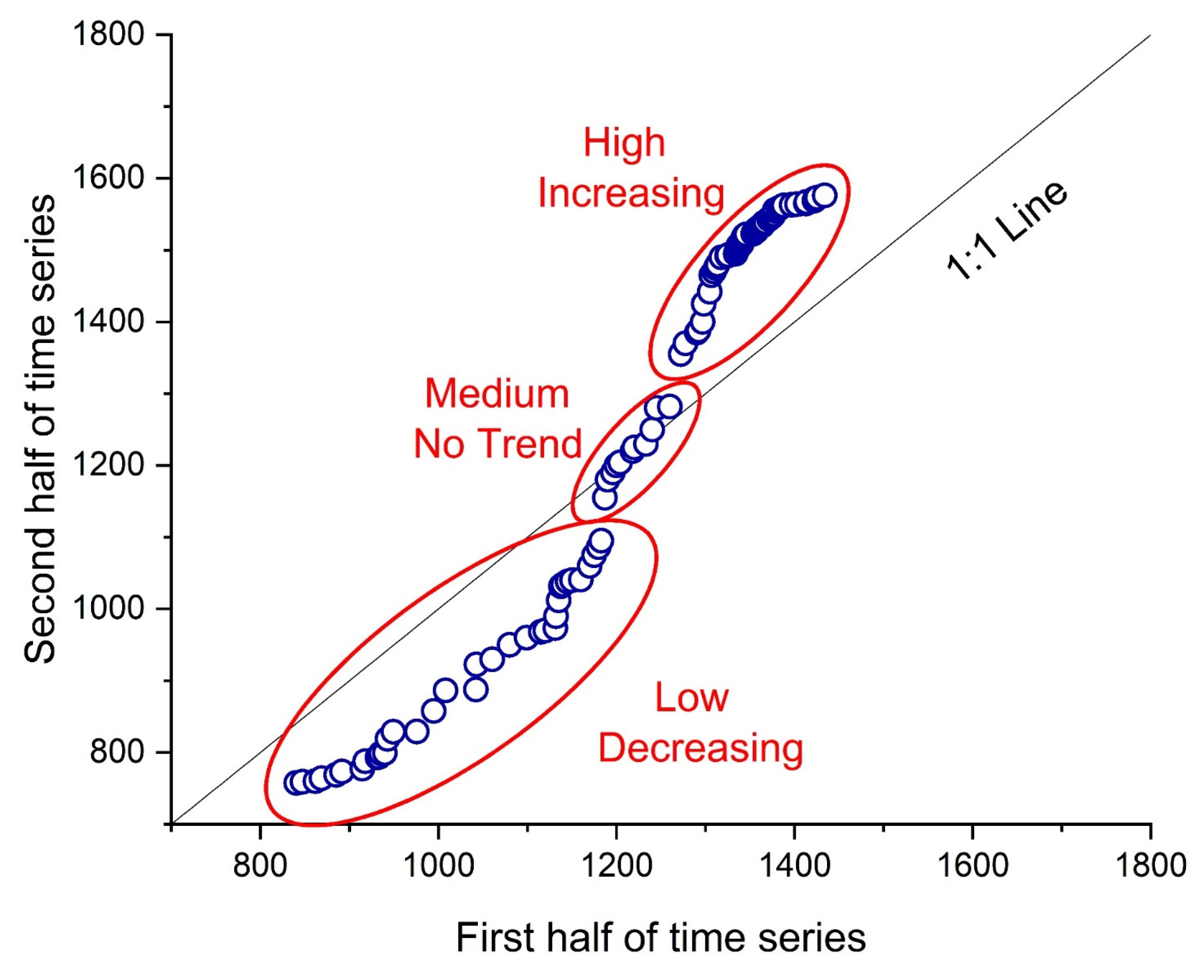
Innovative trend analysis, developed by Şen (2012) [35], is a method which examines the trends of the time series dataset by plotting a graph with advantages in detecting the trend in the low, medium and high values in a time series. This method can be accomplished by the following steps:

(1) For a time series dataset $T$, we divide this time series data into two equal parts ($T_1$ and $T_2$). T1 is the first half of the time series dataset and $T_2$ is the second half of the time series dataset. This situation is applied when the length of the time series dataset is an even number. If the number of time series data is odd, remove the first record of the time series data.

(2) The two parts ($T_1$ and $T_2$) of the time series dataset are sorted by increasing sequence of the value, separately.

(3) A scatter diagram is plotted by using the first half of the time series dataset $T_1$ as the X-axis and the second half of the time series dataset as the Y-axis.

(4) Plot 1:1 reference line in the scatter diagram.

(5) Identifying the time series trend using the evaluation rules below.

An increasing trend is presented if the scatters are distributed above the 1:1 reference line. A decreasing trend is presented if the scatters are distributed below the 1:1 reference line. No trend is presented if the scatters are distributed on the 1:1 reference line. The above three situations show that the time series dataset is a monotonous trend. In fact, a non-monotonous trend also existed in some time series datasets; that is to say, a mixture of the above three situations may appear simultaneously. A diagrammatic drawing is shown in Figure 2. In this situation, we separate the scatter into three parts including the low value part, medium value part and high value part, and identify the trend in the time series in the same way as the time series data with a monotonous trend.

The slope of the time series dataset can by calculated by Equation (1):

$$Slope=\frac{2\left(\overline{T_2}-\overline{T_1}\right)}{n}$$

(8)

where $\overline{T_2}$ is the average value of the second half of the time series dataset, $\overline{T_1}$ is the average value of the first half of the time series dataset, and n is the length of the time series data.

2.3.4. HARTT Model

The HARTT (Hydrograph Analysis: Rainfall and Time Trends) model is a statistical method to estimate the trends in the groundwater level. It was developed by Ferdowsian et al. (2001) based on CDFM (cumulative deviation from mean) which is based on the estimation of the cumulative departure from mean rainfall over the period of monitoring [39,51]. The HARTT model is a useful tool in groundwater resource modelling, and it has the following advantages: (1) it is simple and useful; (2) it separates the influence of atypical rainfall events on groundwater level changes from the time series; (3) the lag time of the rainfall event on groundwater level changes can also be calculated; (4) the results of the HARTT model are consistent with the intuitive hydrological explanations; and (5) simulation results are reliable for bores with depths greater than 5 m [39,52]. A potential disadvantage of the HARTT model is the rainfall in the observation periods is not in accordance with the typical long-term average rainfall [51]. Rainfall in the HARTT model is represented as accumulative residual rainfall. Two expressions of accumulative residual rainfall can be used. Accumulative monthly residual rainfall (AMRR, mm) is the first one, and it is expressed as Equation (9):

$$AMR{R}_t={\displaystyle \sum }_{i=1}^t\left(M_{i,j}-{\overline{M}}_j\right)$$

(9)

where $AMR{R}_t$ is the accumulative monthly residual rainfall at time t. $M_{i,j}$ is the ith month rainfall of the total rainfall time series which corresponds to the jth month of one year. ${\overline{M}}_j$ is the average monthly rainfall at the jth month of the year. t is the total months from the first record to the end record. The fluctuation of AMRR is relatively low within a year, because the fluctuation in the actual rainfall is offset by the seasonal variation of the average monthly rainfall.

The accumulative annual residual rainfall (AARR, mm) is the second one, and it is expressed as Equation (10):

$$AAR{R}_t={\displaystyle \sum }_{i=1}^t\left(M_i-\overline{A}/12\right)$$

(10)

where $AAR{R}_t$ is the accumulative annual residual rainfall at time t, $M_i$ is the ith month’s rainfall from the beginning of the time series, and $\overline{A}$ is the long-term average monthly rainfall.

$$D\mathrm{e}pt{h}_t=k_0+k_{1}AMR{R}_{t-L}+k_{2}t$$

(11)

$$D\mathrm{e}pt{h}_t=k_0+k_{1}AAR{R}_{t-L}+k_{2}t$$

(12)

where $D\mathrm{e}pt{h}_t$ is the groundwater level at time t. L (unit: month) is the lag time between the rainfall event and its impact on the groundwater level. k₀, k₁ and k₂ are the parameters to be estimated. Parameter k₀ is approximately equal to the initial groundwater level. k₁ represents the impacts of rainfall that is higher or lower than the average rainfall on the groundwater level. k₂ represents the rate of the increasing or decreasing trend in groundwater level over time. t is the months from the beginning to the end of the groundwater level time series.

3. Results and Discussion

3.1. Intra-Annual Variation in Groundwater Level

A trend analysis of the monthly groundwater level from 1977–2017 in the Gnangara region was conducted in the present study with over 20 years of observation head data from 1977 to 2017. A Mann–Kendall test and Sen’s slope estimator have been used for the determination of the trend and the trend magnitude.

3.1.1. Variation in Average Monthly Groundwater Level

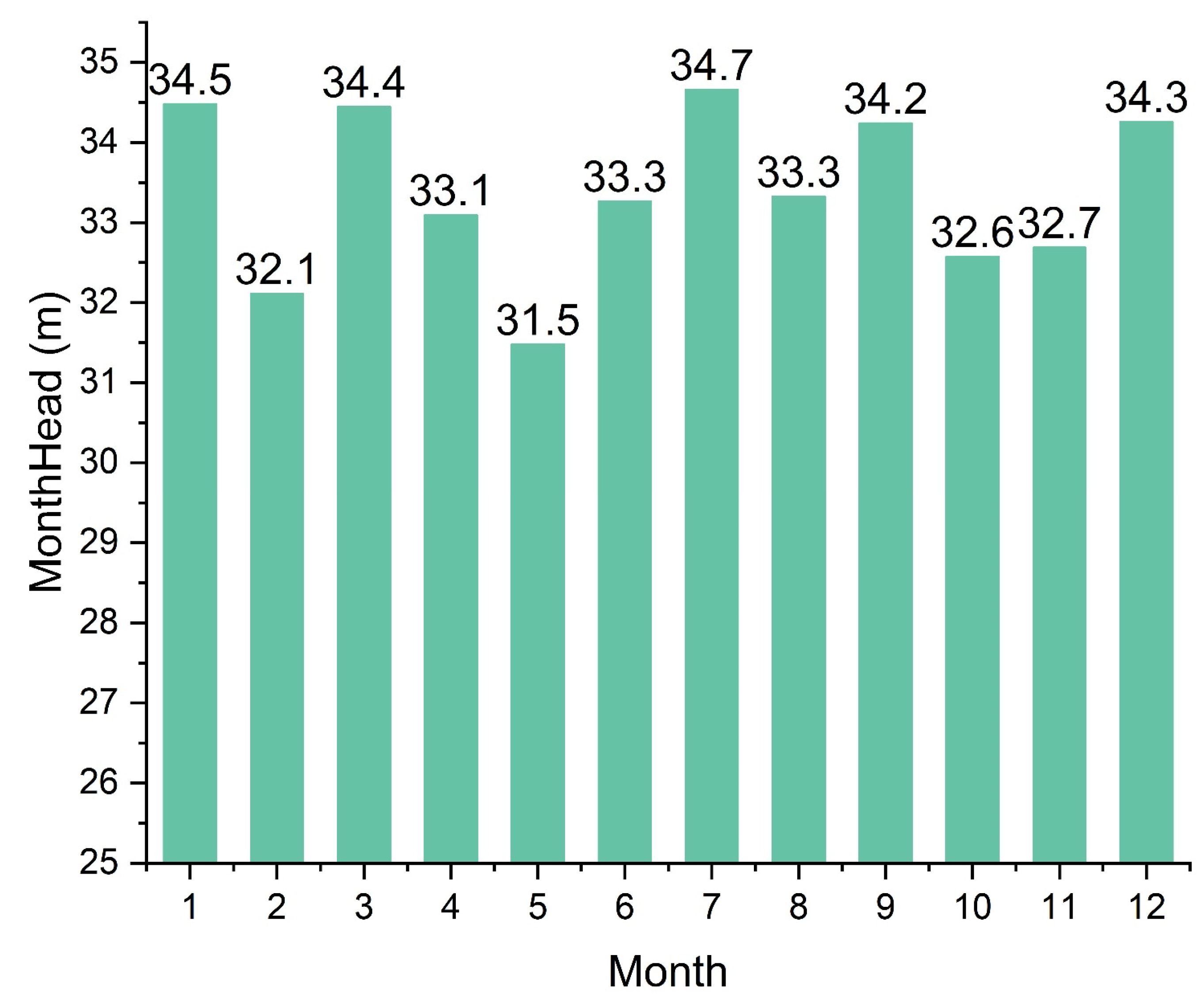
The average monthly groundwater level in the Gnangara region was calculated by averaging the monthly groundwater level of 351 bores during 1977–2017. The results are shown in Figure 3. The lowest average monthly groundwater level of 31.5 m occurred in May and the highest average monthly groundwater level of 34.7 was found in July. There was no seasonal trend in the average monthly groundwater level of the Gnangara region.

3.1.2. Long-Term Variation in Monthly Groundwater Level

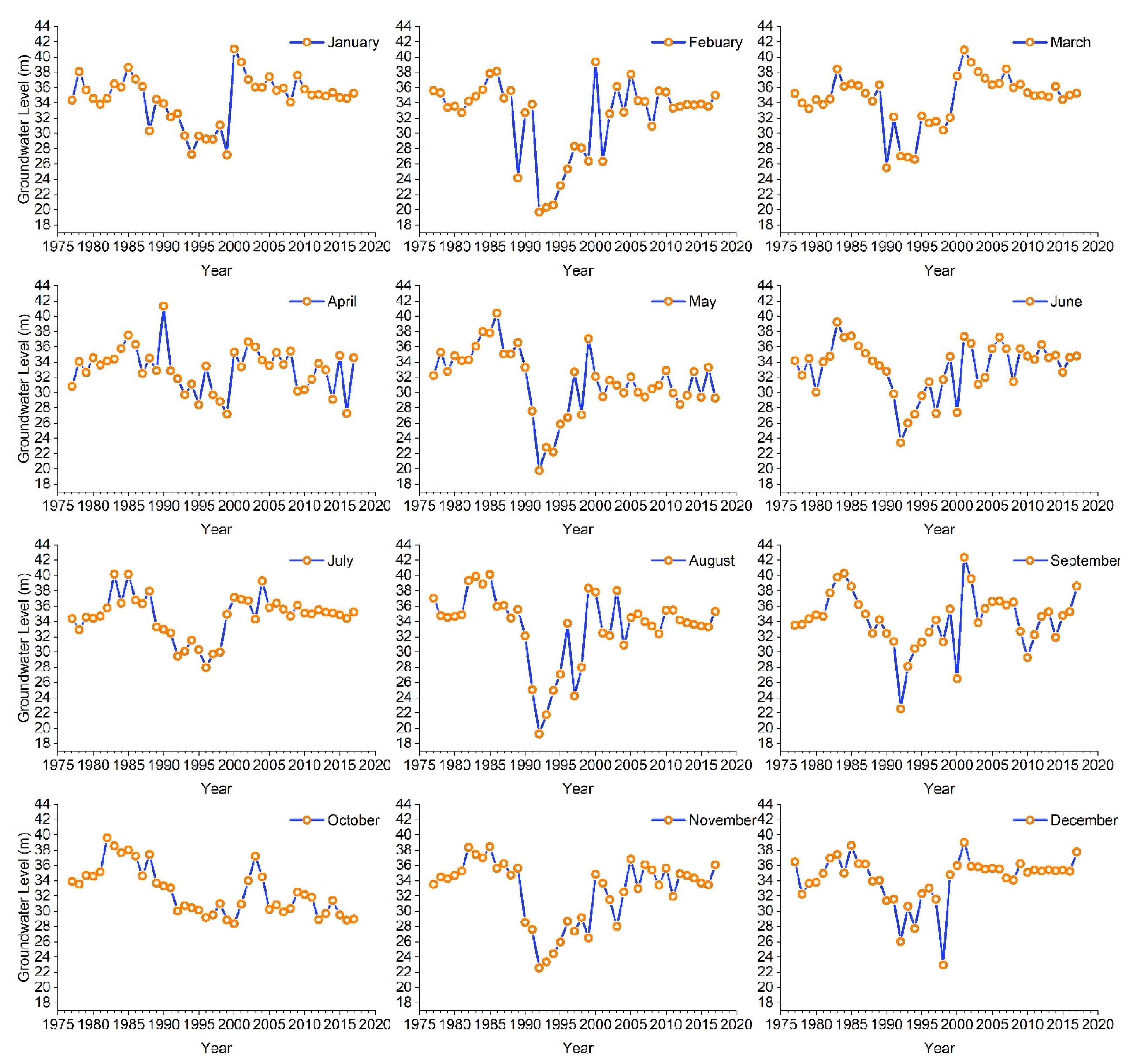
In order to analyze the variation trend in the groundwater level of each month of the year from 1977 to 2017, the average monthly rainfall of the Gnangara region from 1977 was plotted in Figure 4. The fluctuation in the groundwater level in April, July and October was slight. The groundwater level in other months fluctuated greatly. From 1977 to 1984, the groundwater level was high with a slightly increasing trend. Since 1985, the groundwater level in each month tended to decrease. Until 1992, the groundwater level in most months reached the lowest value except for the groundwater level in January, April and October, for which the lowest values occurred around 1999. From 1993 to 2001, the groundwater level showed an increasing trend again. After 2001, the groundwater level in each month tended to be stable.

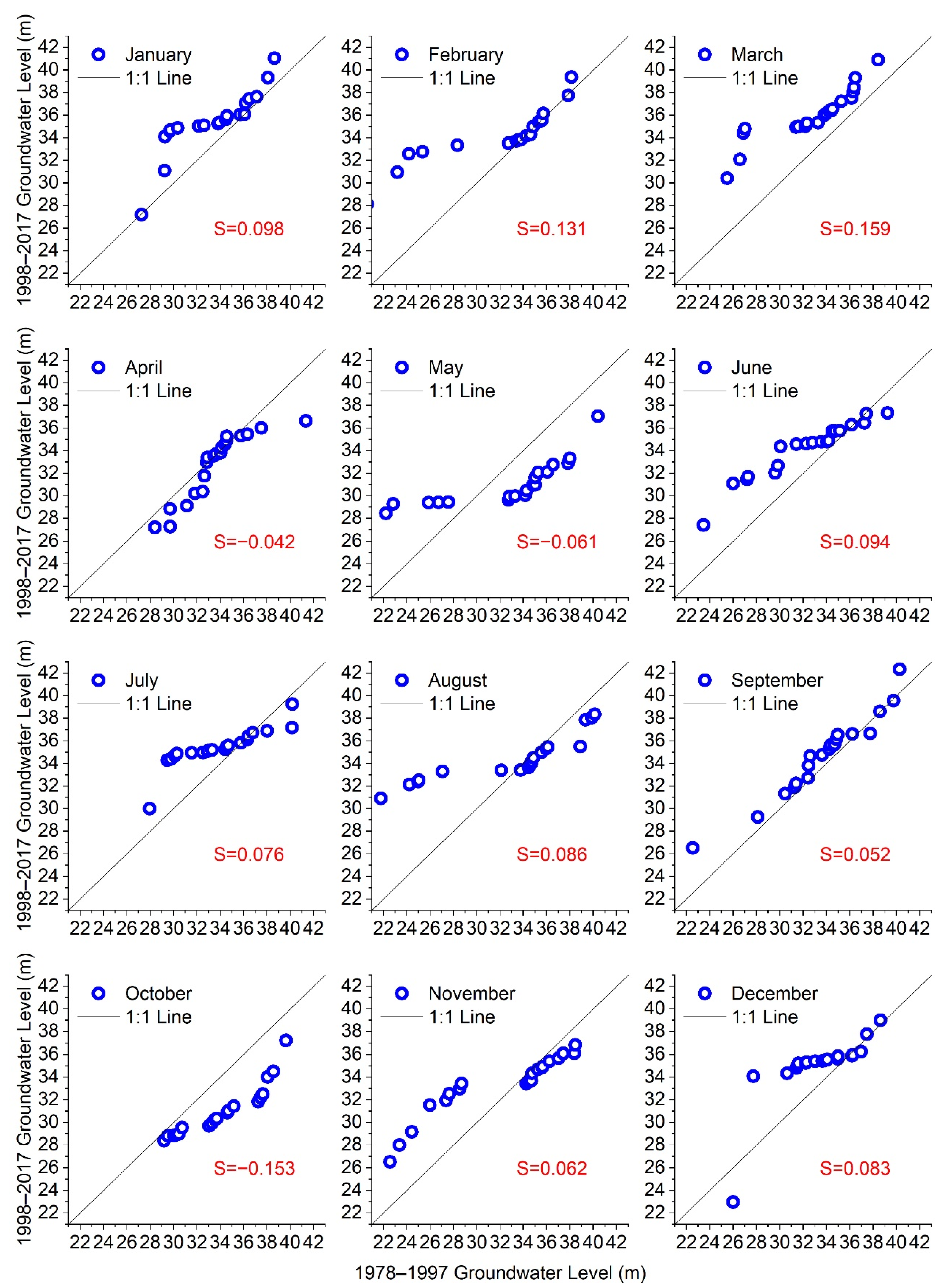
The innovative trend analysis method was used to analyze the trend in groundwater level in each month and the results are shown in Figure 5. Scatters of groundwater level from December to March in the next year were distributed above the 1:1 reference line, indicating an increasing trend in groundwater level in these months during the period 1998–2017 compared to the same months during the period 1978–1997. In addition, the groundwater level in the Gnangara region showed a strong increasing trend at a low groundwater level and the slopes were 0.083, 0.098, 0.131, 0.159 for December, January, February and March, respectively. In April and October, scatters were distributed below the 1:1 line, demonstrating the decreasing trend in groundwater level, and the slopes were −0.042 and −0.153, respectively. In May, June, July, August and November, scatters with a low groundwater level were distributed above the 1:1 line and scatters with a high groundwater level were distributed below the 1:1 line, especially in May, August, and November. This illustrated that groundwater level in the Gnangara region had a non-monotonic trend in these months and showed an increasing trend at a low groundwater level and a decreasing trend at a high groundwater level. In addition, the slope trends in these months were −0.061, 0.094, 0.076, 0.086 and 0.062, respectively. In September, scatters are distributed around the 1:1 line, indicating a stable groundwater level.

3.2. Inter-Annual Variation in Groundwater Level

3.2.1. Long-Term Variation in Annual Mean Groundwater Level

The mean annual groundwater level in each bore was spatially averaged to detect the variation trend in the groundwater level in the whole Gnangara region.

The long-term trend in groundwater level in the Gnangara region was analyzed by a Mann-Kendall test and Sen’s slope. The statistic Z is −6.4134 (p < 0.01) and Sen’s slope is −0.145, indicating the significant decreasing trend in groundwater level in the Gnangara region. The linear regression also resulted in the same significant decreasing trend in groundwater level with a slope of −0.16 (R² of 0.76, adjusted R² is 0.76) (Figure 6).

3.2.2. Variation in Annual Mean Groundwater Level in Different Periods

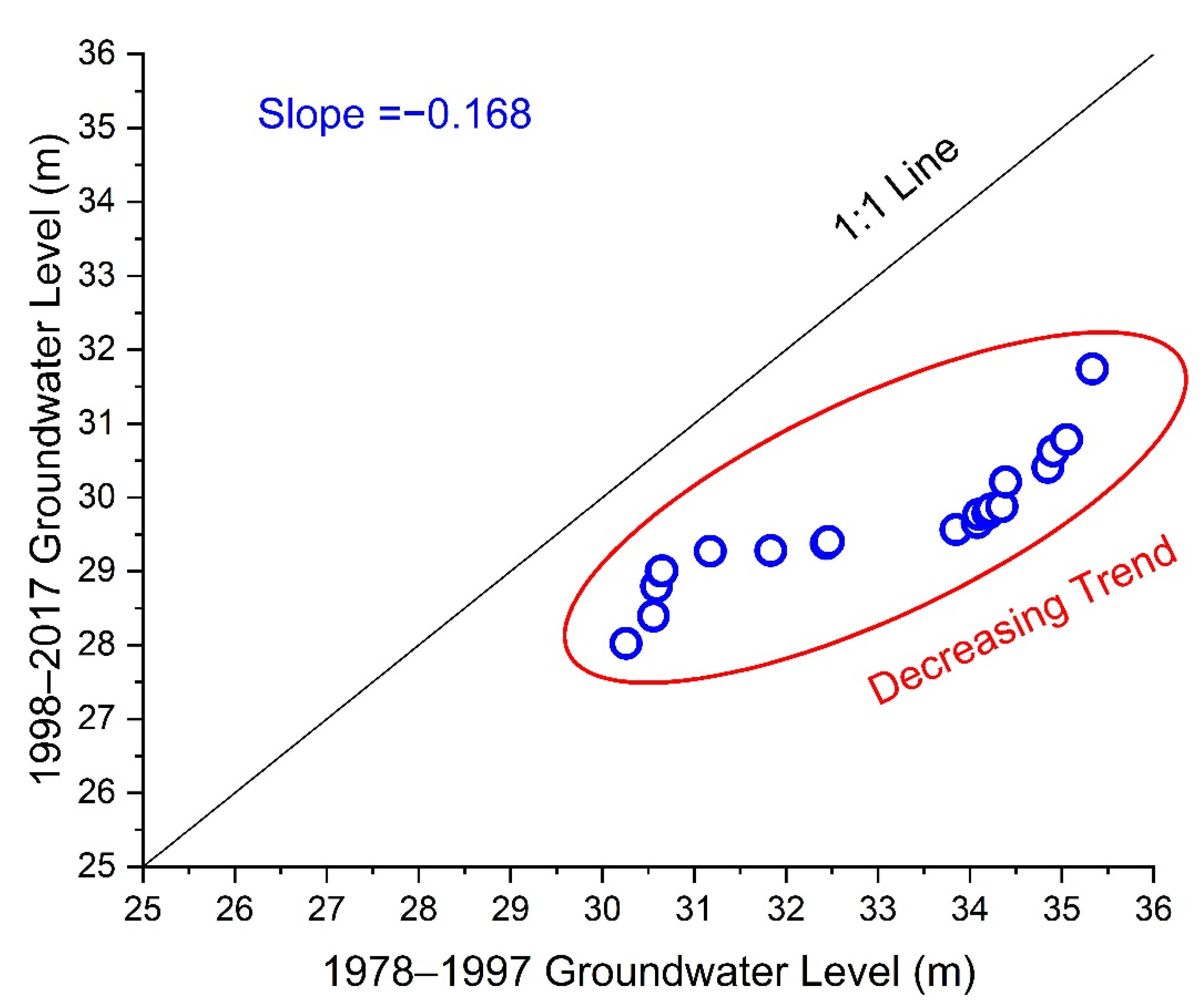
The innovative trend analysis was used to analyze the groundwater level trend. First of all, the data in 1977 were removed because the lengths of the groundwater level data were odd, and the groundwater level time series from 1978 to 2017 is divided into two equal parts (1978–1997 and 1998–2017). Secondly, these two time series datasets were sorted by an increasing sequence of the groundwater level observations. Then, a scatter plot was drawn using a groundwater level time series dataset in 1978–1997 as the X-axis and a groundwater level time series dataset in 1998–2017 as the Y-axis. Lastly, a 1:1 reference line was plotted in the scatter plot to analyze the trend in the groundwater level time series dataset. The results of the innovative trend analysis on groundwater level were shown in Figure 7. Groundwater level in the Gnangara region showed a monotonic trend in the period of 1998–2017 compared with 1978–1997. The largest and lowest groundwater levels are 30.26 m and 28.02 m, respectively, and all the scatters are distributed below the 1:1 line, demonstrating the decreasing trend in the groundwater level in the Gnangara region. Additionally, there is a big distance between scatters with a high groundwater level and 1:1 line, indicating a stronger decreasing trend at the high groundwater level than at the low groundwater level. The slope of the decreasing trend is −0.168. These results suggest that there is no big difference between the innovative trend analysis and linear regression to analyze the trend in groundwater level.

3.3. Spatial Variation in Groundwater Level

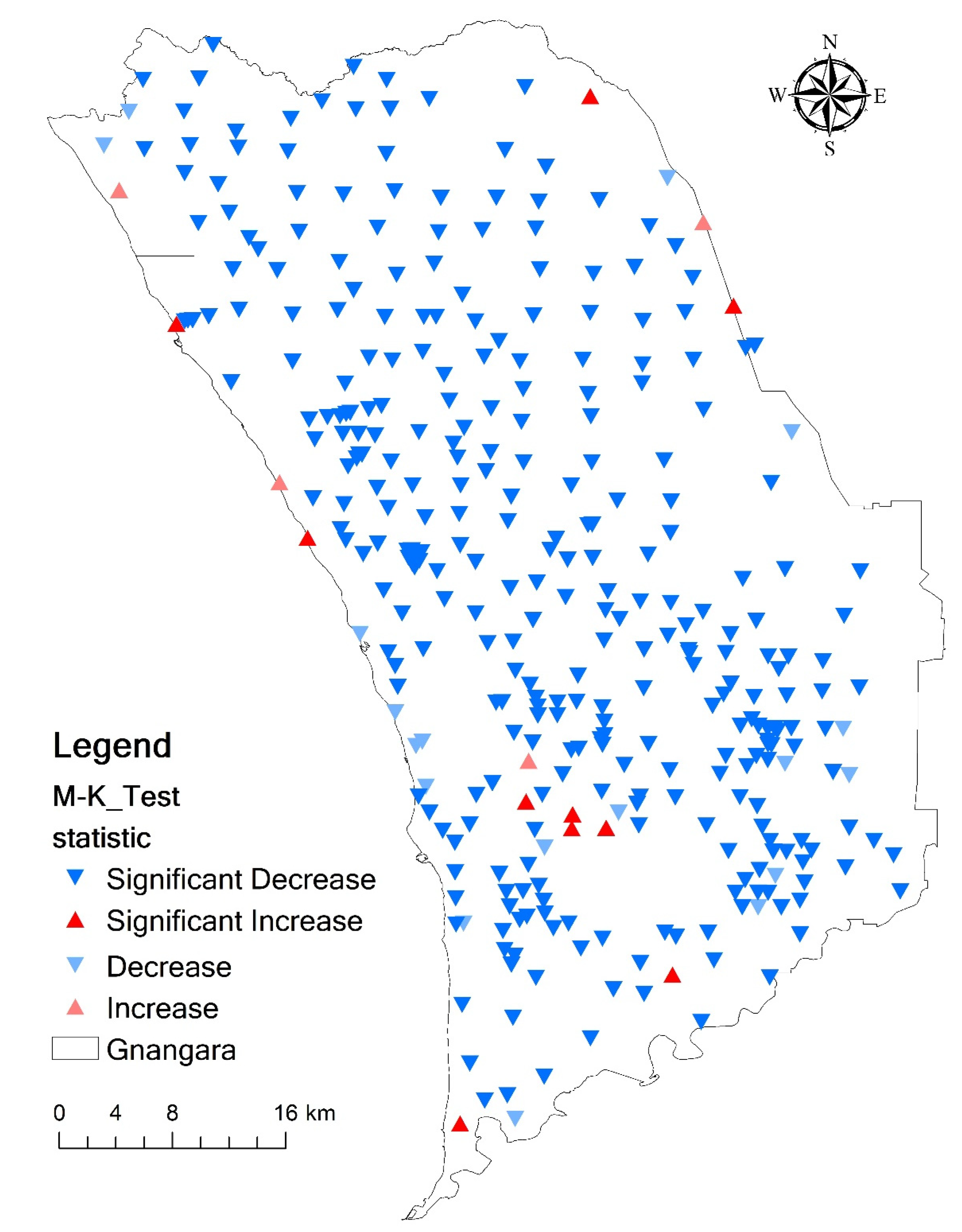
The trend analysis of groundwater level data was carried out by applying the MK test at annual time scales. Figure 8 showed the groundwater level trend results at 351 observation bores. A total of 336 observation bores exhibited a decreasing trend in groundwater level and 15 observation bores exhibited an increasing trend in groundwater level. The MK test detected a statistically significant trend in groundwater level in 329 out of 336 observation bores at a 95% significance level. Fifteen observation bores did not show a trend that was statistically significant. Statistically significant decreasing trends were observed at 319 observation bores (91%) in most areas of the Gnangara region and statistically significant increasing trends were detected at 10 bores (3%) (significant level at 0.05), which were located in the northwest, northeast margin, and southwest areas of the Gnangara region.

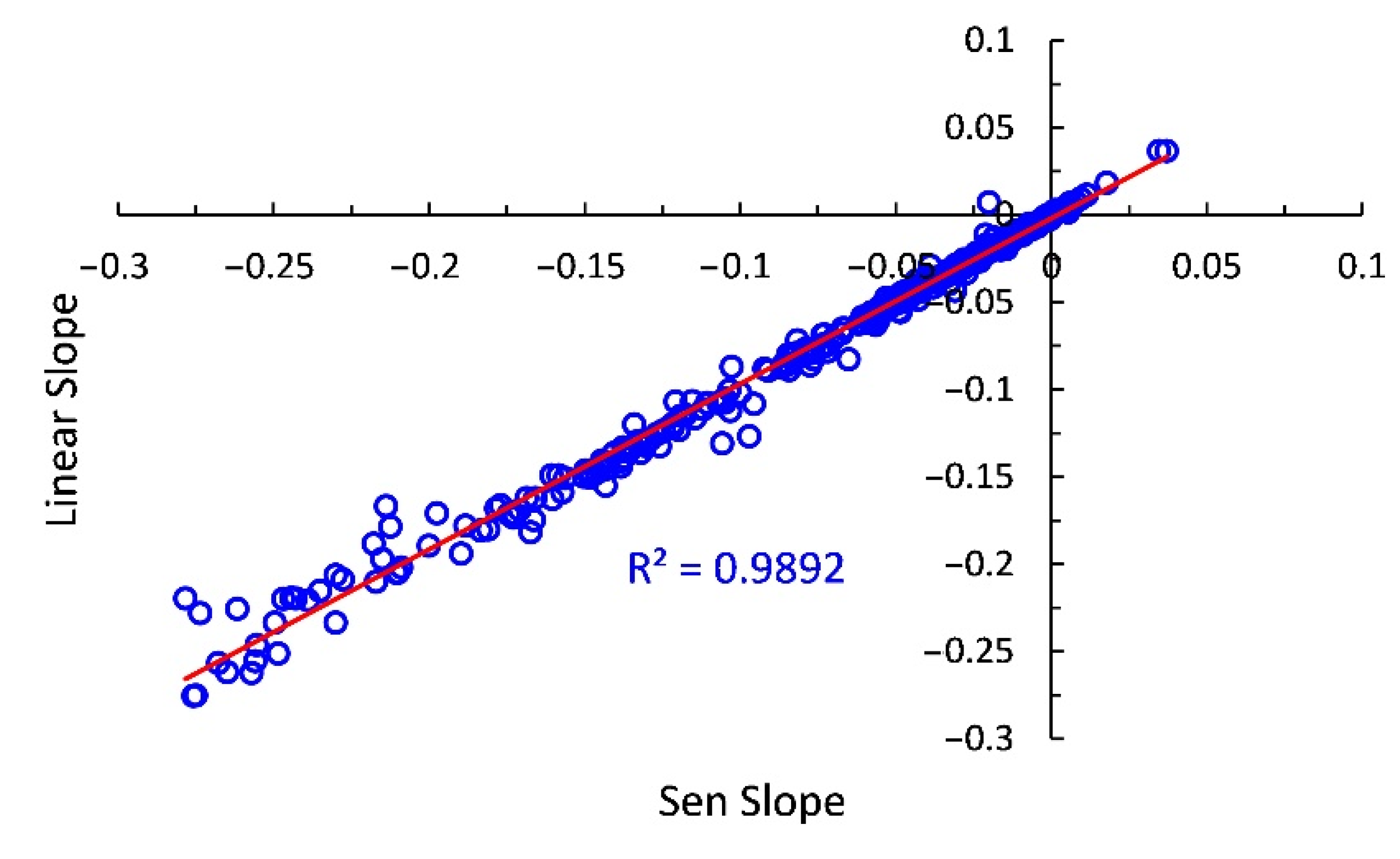
The magnitude of statistically significant trends at an annual scale was determined using the Sen’s slope estimator. Figure 9 showed there was no big difference between the results of the linear trend and Sen’s slope. The magnitudes of the significant decreasing trends in annual groundwater level are less than −0.28 m/year. The magnitudes of the significant increasing trends in annual groundwater level ranged between 0–0.03 m/year. According to the relationship between trend magnitude and groundwater level (Figure 10), the small trend magnitudes were found in groundwater levels of 0–10 m and 60–80 m and the big trend magnitudes were found in groundwater levels of 10–60 m.

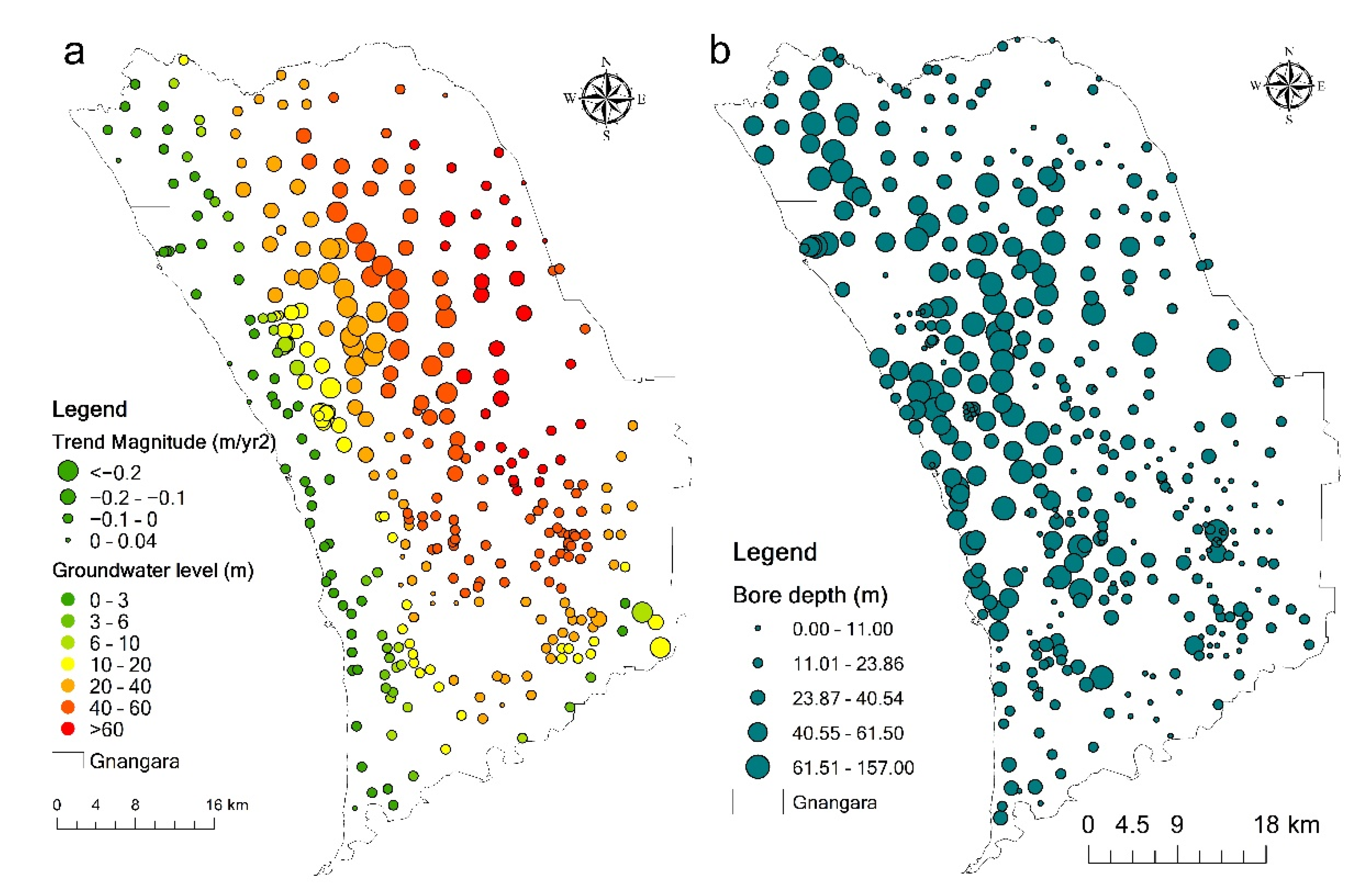
A trend map prepared from the results of Sen’s slopes by ArcGIS 10.2 was used to interpret the spatial distribution of trends in the groundwater level in the Gnangara region (Figure 11). Generally, the groundwater level in the Gnangara region was dominated by a downward trend, and the trend increased from the margin of the Gnangara to the central part of northern Gnangara. In the west, east margin area and southern Gnanagara region, a small number of bores (4%) showed an increasing trend in the groundwater level with a trend rate ranging from 0 to 0.04 m/year. About 68% of bores in the margin and southwestern area of the Gnangara showed a decreasing trend in the groundwater level with a rate of decline ranging between −0.1~0 m/year. Along the margin of the Gnangara region, about 19% of the bores had a decreasing trend in the groundwater level with a trend rate ranging between −0.2 and −0.1. About 8% of the bores in the central area of northern Gnangara showed a statistically significant decreasing trend in the groundwater level with a rate of decline of less than −0.2 m/year.

The mean annual groundwater level was lowest in the western coast and south of the Gnangara region, with a value of less than 3 m, and the groundwater level increases up to more than 60 m from the west to east and from the south to north.

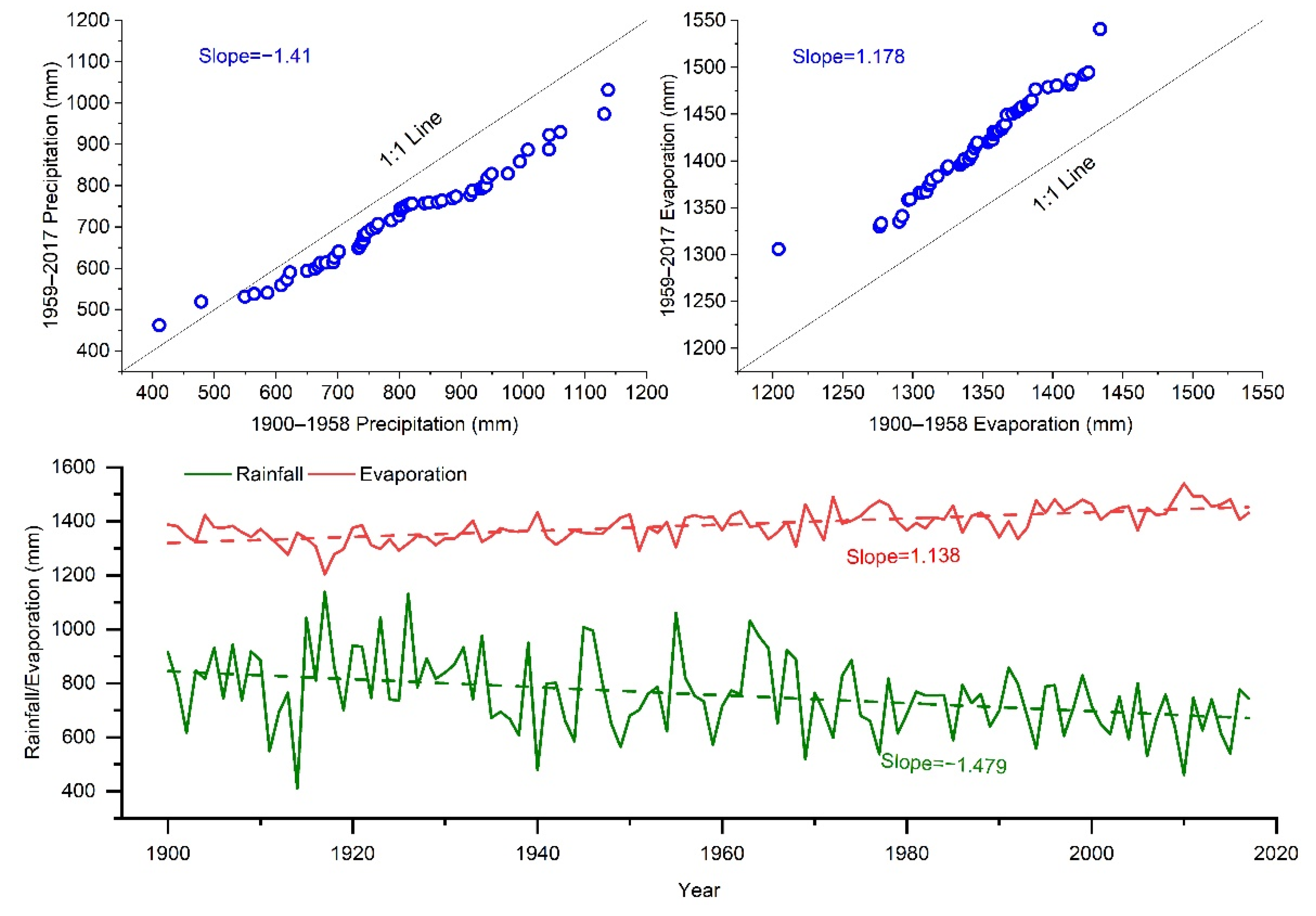
In order to analyze the influences of climate change on the dynamic changes in groundwater level, linear regression and the innovative trend analysis were applied to the mean annual rainfall and mean annual evaporation, and the results were shown in Figure 12. Scatters of the rainfall were mainly distributed below the 1:1 line and scatters of the evaporation were distributed above the 1:1 line, illustrating the decreasing trend in rainfall (slope: −1.41) and increasing trend in evaporation (slope: 1.178) in 1959–2017 compared to 1900–1958. Linear regression also resulted in the same decreasing trend in rainfall and increasing trend in evaporation from 1900 to 2017, with slopes of 1.479 and 1.138, respectively (Figure 12).

Rainfall is the main source of groundwater, and evaporation can reduce the groundwater level by intensifying the hydrological cycle [53]. Groundwater level decline in the Gnangara region was closely related to the reduction in rainfall and increase in evaporation. However, the changing trend rate of the groundwater level (−0.16) was lower than the rate of the rainfall (−1.479), indicating that there are other factors such as groundwater abstraction, land use and land cover changes that may influence the groundwater level in the Gnanagara region.

3.4. Relationship between Rainfall and Groundwater Level

Results of the monthly rainfall variation from 1977 to 2017 were shown in Figure 13. From October to April in the next year, rainfall in the Gnangara region was low with a value of less than 100 mm, and the rainfall showed slight fluctuation, especially in December. From May to September, rainfall was abundant with a value of more than 50 mm and greatly fluctuated, especially in May to July. Both monthly groundwater level and annual groundwater level showed a temporary increasing trend in the early 1980s, a dramatically declining trend since about 1985, and a sharp increasing trend in the early 2000s (Figure 4). However, monthly rainfall did not show big changes in these periods, suggesting that the groundwater level in these periods may have been influenced by other factors.

The vegetation of pine plantations and Banksia wood are the main forms of land use in the central area. In the early 1980s, the local trees were cleared gradually, and the pine trees were planted for commercial use. Moreover, studies have shown that pine trees consume more water than local trees, which had resulted in sharp decreases in the groundwater level in the late 1980s and early 1990s. From the early 2000s, the pine trees were cleared and replaced gradually by local trees, and the groundwater level showed a temporary recovery.

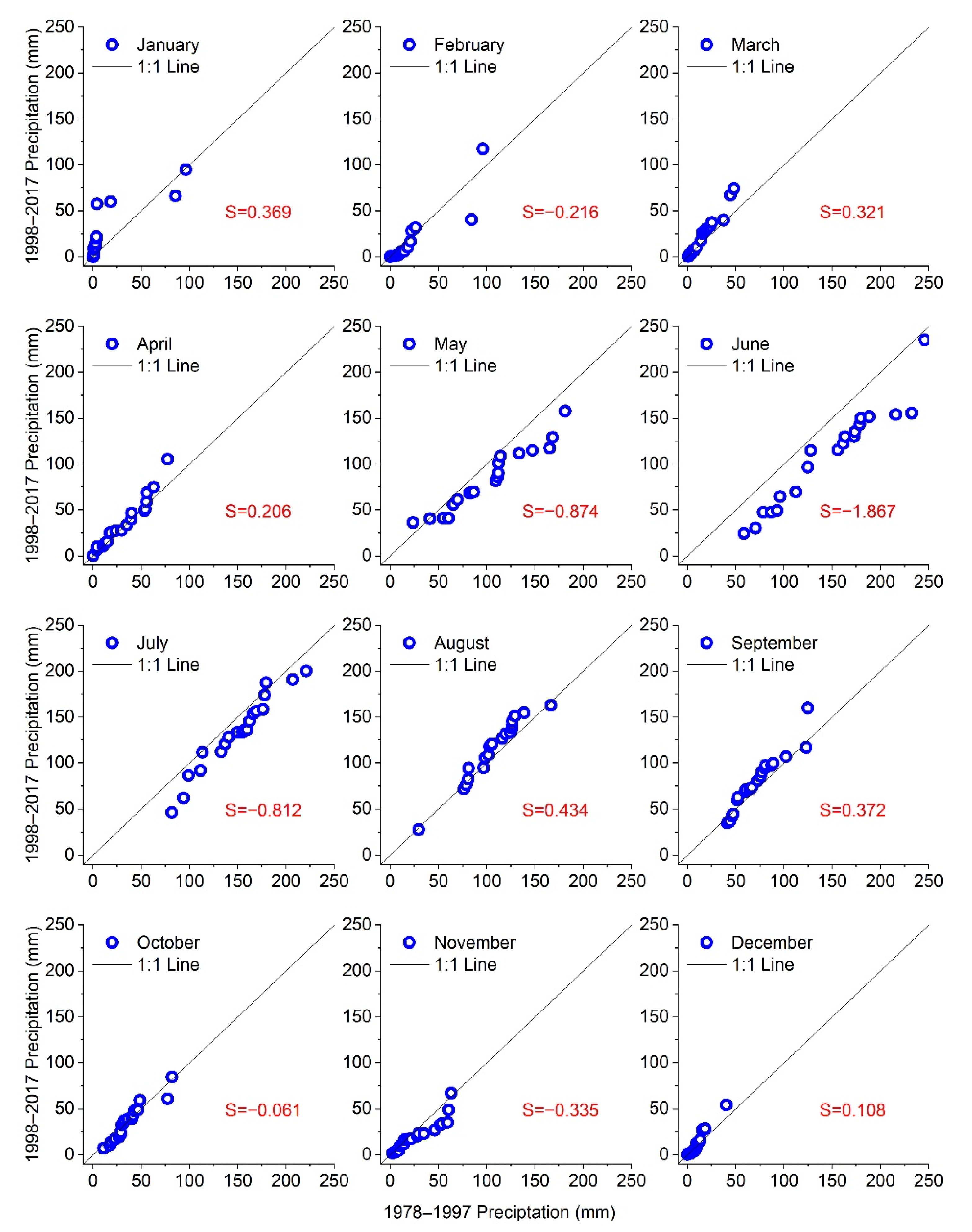
The results of the innovative trend analysis on the monthly rainfall were shown in Figure 14. In January, March, April and December, rainfall scatters were concentrated in the low value area and distributed above the 1:1 line, indicating a slightly increasing trend in rainfall in 1998–2017 compared to 1978–1997 with trend rates of 0.108, 0.369, 0.321 and 0.206, respectively. From May to July and October to November, rainfall scatters were mainly distributed below the 1:1 line, indicating a decreasing trend in 1998–2017 compared to 1977–1997. In addition, many rainfall scatters in May to July were mainly distributed in the high rainfall value area of Figure 14 and was a departure from the 1:1 line, demonstrating a large decreasing trend with slopes of −0.874, −1.867 and −0.812, respectively. Contrary to the rainfall scatters in May to July, the rainfall scatters in October to November were mainly distributed in the low rainfall value area of Figure 14, indicating a small decreasing trend with slopes of −0.061 and −0.335, respectively. Comparing the changing trend between groundwater level and rainfall, the same increasing trend occurred in January, March, August, September and December and the same decreasing trend occurred in May and October. It is worth noting that the contrary changing trend between groundwater level and rainfall occurred in February, April, June and November. In the Gnangara region, rainfall had significant influences on the groundwater level according to the above trend analysis between groundwater level and rainfall.

3.5. Rainfall Impacts on the Groundwater Level Based on the HARRT Model

3.5.1. Rainfall Patterns

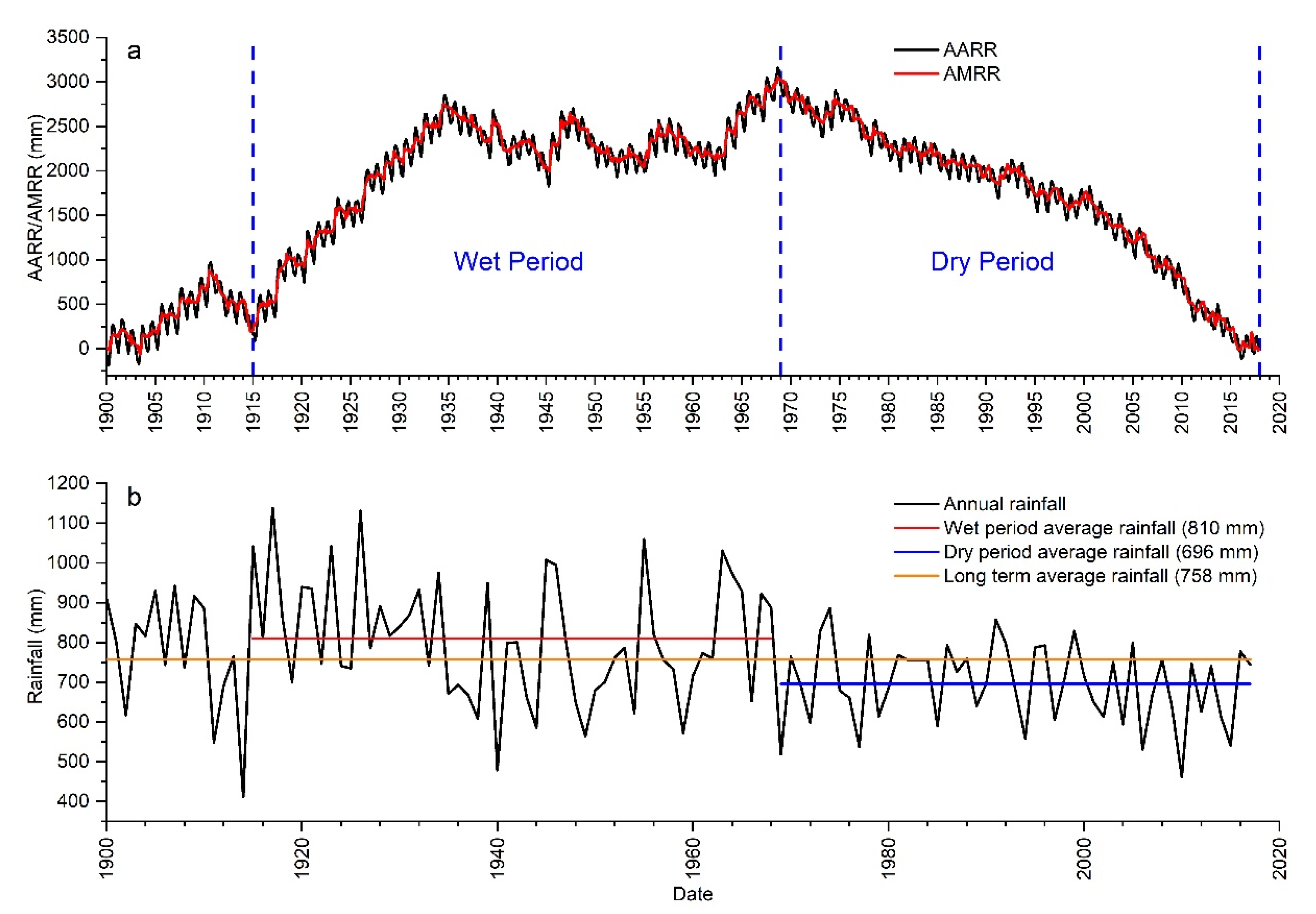
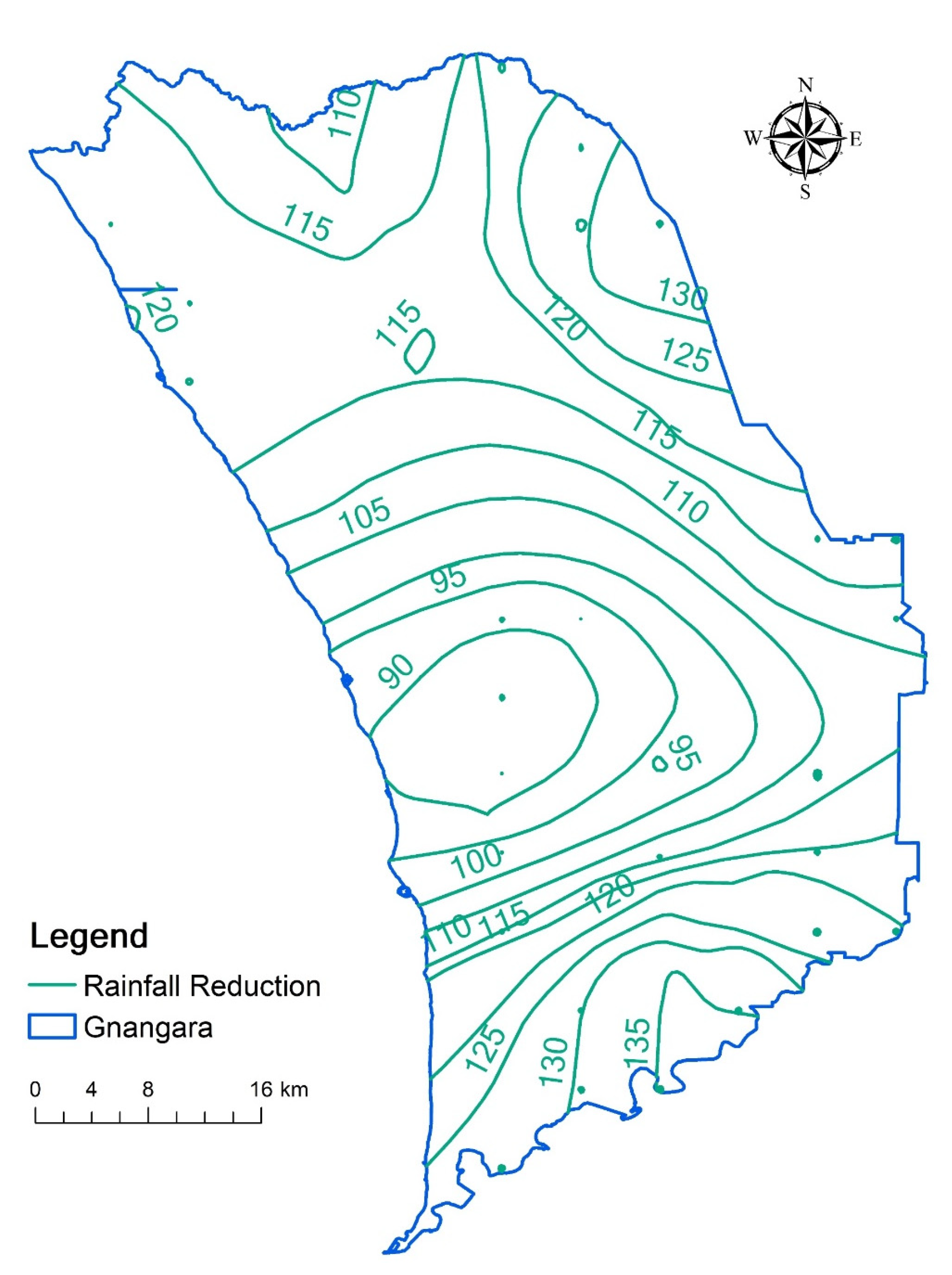
The rainfall pattern was evaluated using the HARRT technique, which determined a wet period between 1915 and 1968, and a dry period following 1969 (Figure 15a). From 1915, the AARR and AMRR showed an increasing trend with fluctuations, and it reached a peak value of mm until 1969. After that, the AARR and AMRR turned to be continually decreasing trends. These periods were the same with the results of cumulative deviation from the mean rainfall (CDFM) analysis conducted by Yesertener (2007) [54]. Additionally, Yesertener (2007) [54] insisted that the dry period may be a natural climatic phenomenon (reflecting the same pre-1915 condition) or it could be representative of the enhanced greenhouse effects. The reduction in rainfall for the Gnangara region can also be seen in Figure 15b by comparing the long-term (758 mm), wet period (810 mm), and dry period (696 mm) annual mean rainfall values. Rainfall experienced a reduction of 114 mm (14%) in annual rainfall in the dry period when compared to the wet period.

One hundred and eighteen SILO data points were used to determine the distribution of the reduction in annual rainfall in the dry period compared to that in the wet period and the results are given in Figure 16. In the whole region, the rainfall showed a decreasing trend (Figure 16). The annual rainfall in the Gnangara region experienced a 9.5% to 19.7% reduction in the dry period when compared to the wet period. The minimum rainfall reduction of approximately 90 mm was mainly distributed in the lower central-west area. The rainfall reduction increased outward from the point of minimum value. A maximum rainfall reduction of more than 100 mm was mainly distributed in the southeastern and northeastern Gnangara.

3.5.2. Rainfall Impacts

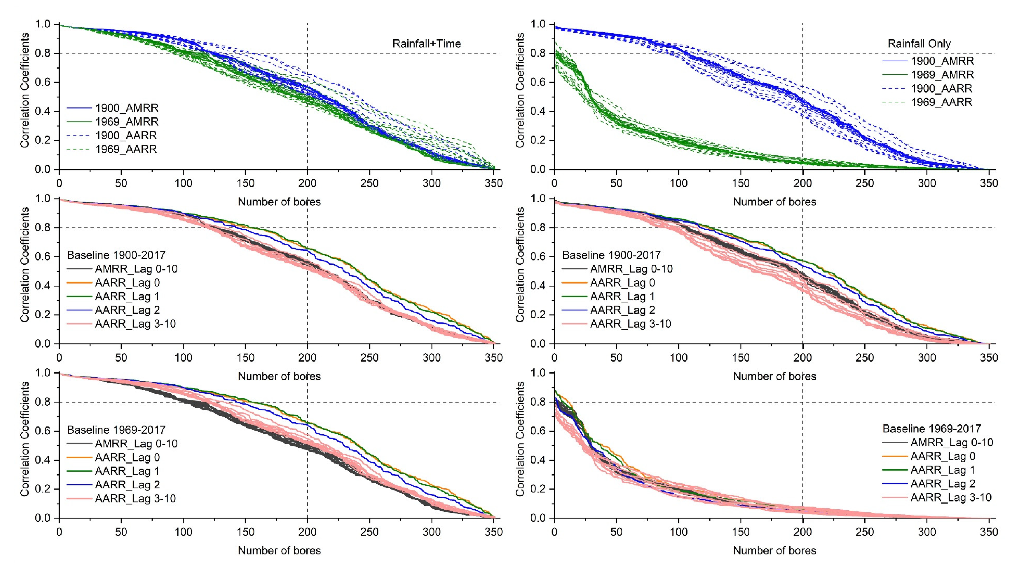
Two models, the rainfall only model and the rainfall and time model (rainfall + time), were compared to choose the best fitted model in the Gnangara region. This study simulated groundwater levels based on the long term (1900–2017) and dry periods (1969–2017) due to the different rainfall patterns before 1968 and after 1968. In addition, there is a lag period for the influence of rainfall on the groundwater level, and the lag period in this study area is uncertain; therefore, the study attempted 11 lag periods measured in months (from 0 month to 10 months) to determine the lag period of the influence of climate on the groundwater level. Results are shown in Figure 17.

For the rainfall only model, during the period of 1900–2017, the correlation coefficient curve based on the AARR and AMRR protruded to the upper right. However, during the period of 1969–2017, the correlation coefficient curve protruded to the lower left. For the rainfall + time model, the correlation coefficient curve based on the AARR and AMRR protruded to the upper right during the period of 1969–2017. This demonstrated that the accuracy of the model was promoted when the time variable was considered in the model. In addition, the correlation coefficient between rainfall and groundwater level is higher in the period of 1900–2017 than 1969–2017 for both the rainfall only model and the rainfall + time model, which indicated that the period of 1900–2017 is more fitted to the HARTT model to analyze the rainfall’s impacts (k₁ in Equations (11) and (12)) on the groundwater level.

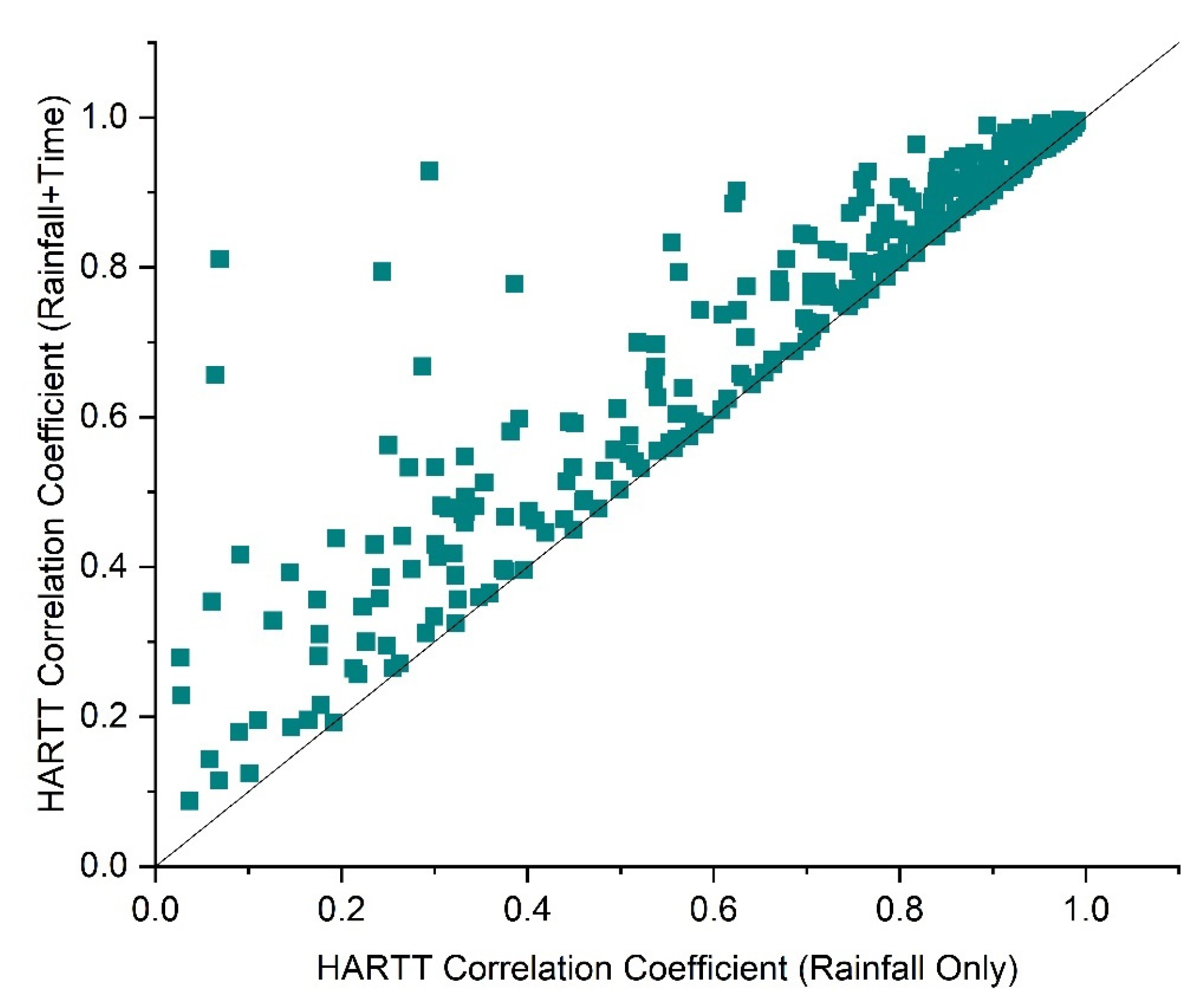
Moreover, for the rainfall only model, AARR with zero-, one- and two-month lag inbaseline 1900 and 1969 showed a better correlation with groundwater level than the AARR with a 3–10 month lag and the AMRR with a 0–10 month lag. The rainfall + time model had the same conclusion as the rainfall only model. Moreover, the simulation results of zero- and one-month lag based on the AARR are better than the two-month lag for the rainfall + time model. These indicated that there is a 0–2 month lag on the influence of rainfall on groundwater level in Gnangara. Furthermore, the number of observation bores with a high correlation coefficient was more in the model with a one-month lag. As Figure 18 shows, the correlation coefficients of the observation bores of the rainfall + time model were mainly distributed above the 1:1 line, indicating better simulation results than the rainfall only model. The AARR in baseline 1900 for the rainfall + time model with a one-month lag had the largest number of bores (156, 44%) with a correlation coefficient greater than 0.8. Therefore, the best model is defined as the rainfall + time HARTT model with a one-month lag based on AARR during 1900–2017.

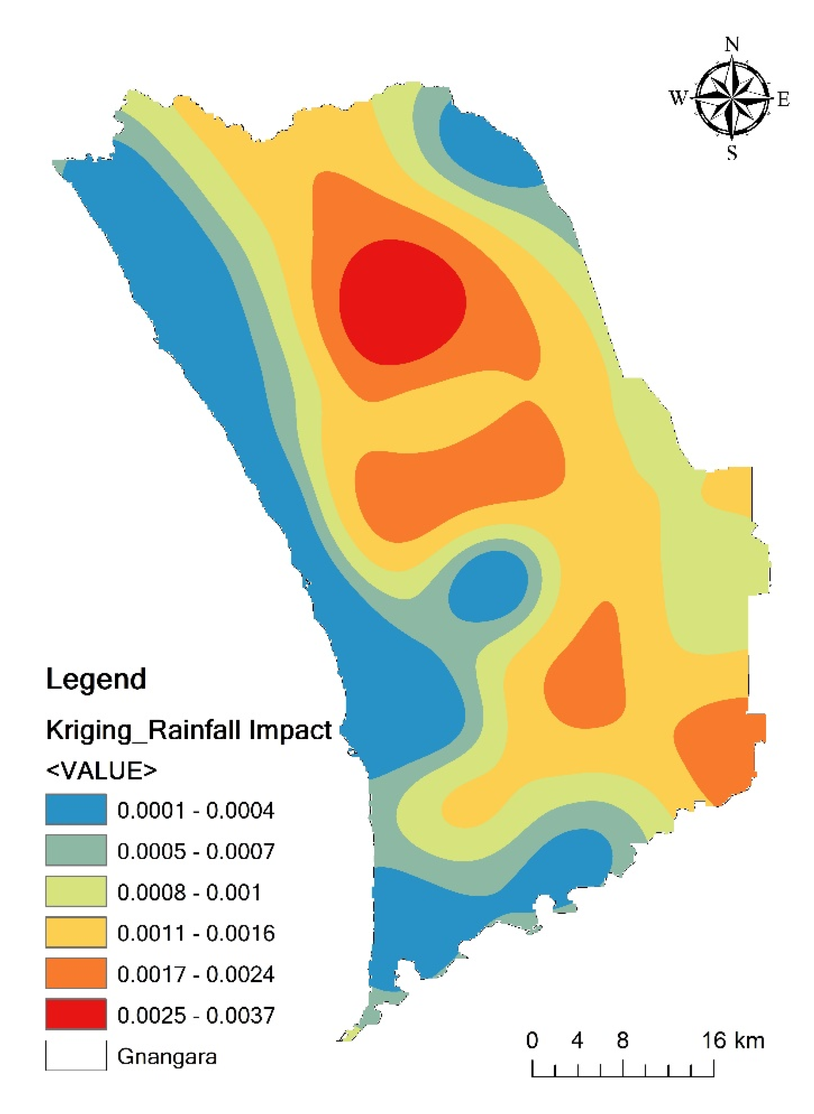
Based on the best HARTT model determined above, the influence coefficients of rainfall on the groundwater level in each observation bore were interpolated by the inverse distance weighted (IDW) method in ArcGIS 10.2. The results were shown in Figure 19. The areas where rainfall had a greater impact on the groundwater level were mainly distributed in the middle of the study area, especially in the middle of the northern part of the study area where rainfall has the greatest impact on the groundwater level with the highest impact coefficient up to 0.00473. From the central part to the surrounding area of the study area, the influence of rainfall on the groundwater level showed a decreasing trend. Compared to the spatial distribution map of groundwater level (Figure 11), rainfall impacts calculated by HARTT are great in the north-central part with a groundwater level more than 20 m and are little in the western coastal areas with a groundwater level at 0 m–6 m.

Comparing Figure 16 with Figure 11, major decreasing trends are located towards the central area for depths >20 m, and towards the southeast corner for shallow depths <20 m. The reduction in rainfall is largest towards the northeast and southeast of the aquifer. This means the decreasing trend in groundwater level in the southeast corner observed in Figure 11 is highly related to the rainfall reduction in this area. However, the decreasing trend in groundwater level also occurred in the central area. This can be attributed to the extensive pine plantation for commercial use in this area (discussed in Section 3.4). In addition, a clear gradient along the coast in terms of rainfall reduction was observed from Figure 16, which does not correlate with the constant value of the trend (−0.2–0.1) in Figure 11a along the coast for shallow depths. Moreover, the rainfall impacts calculated by HARTT also showed little impact on the groundwater level along the coast (Figure 19) where the groundwater level is away from the land surface (Figure 11b). In addition, the Tamala Limestone containing numerous solution channels and cavities occurs along the coastal strip with high hydraulic conductivity and close interaction with sea water, which has a great impact on the groundwater level in this area. Therefore, the impact of rainfall in the coastal area is very limited. In the southwestern Gnangara, rainfall has little impact on the groundwater level, although rainfall reduction is large when comparing Figure 16 to Figure 19. The reduction in the groundwater level in this area resulted from the groundwater abstraction from the aquifer for public and private use. The impact of the reduced rainfall on the decline in groundwater level decreases with proximity to the discharge zones of the mound where water levels are close to the surface. Because the eastern edge of the mound is being controlled by the Gingin scarp and that groundwater levels are close to the surface along Ellen Brook, the maximum groundwater decline resulting from reduced rainfall is shifted farther west. In the eastern edge of Gnangara, rainfall impact is less than the central area. This is because the groundwater level close to the Gingin scarp and the Ellen Brook is close to surface (well depth ranges between 1–20 m).

4. Conclusions

The inter-annual and intra-annual variation trends of the groundwater level in the Gnangara region were analyzed by four trend analysis methods including the Mann–Kendall test, Sen’s slope estimation, linear regression and innovative trend analysis. Then, the HARTT model was used to simulate the groundwater level to investigate the impacts of rainfall on the groundwater level and the lag between rainfall and its impact on groundwater level in the Gnangara region.

Groundwater level in the Gnangara region showed a downward trend from 1977 to 2017 with a trend rate of −0.145, −1.6 and −0.168 for Sen’s slope estimation, linear regression and innovative trend analysis, respectively. The trend magnitude was low at a groundwater level of 0–10 m and 60–80 m, and was high at a groundwater level of 10–60 m, especially at 30–50 m. The trend magnitude increased from the surrounding area to the central-north area (maximum value of −0.28 m/year) of the Gnangara region.

There was no apparent seasonal trend of monthly mean groundwater level in the Gnangara region, with a highest value of 34.7 m in July and a lowest value of 31.5 m in May. During the period of 1977–2017, groundwater level had great fluctuation except for in April, July and October. From 1985, the groundwater level in each month showed a decreasing trend, and the groundwater level reached the lowest value until around 1992. Compared with the period of 1978–1997, the groundwater level from 1998 to 2017 showed an increasing trend in December to March in the next year and a decreasing trend in April and October. The groundwater level in May to August and November showed a non-monotonic trend with an increasing trend at a low groundwater level and decreasing trend at a high groundwater level. In September, the groundwater level presented as stable.

The inter-annual and intra-annual variation trends in the groundwater level in the Gnangara region were closely related to the local rainfall. The rainfall + time HARTT model with a one-month lag based on AARR during 1900–2017 was defined as the best model to simulate the groundwater level by comparing different model structures and parameters. The areas where the groundwater level was greatly influenced by the rainfall was distributed in the central area of the Gnangara region with a maximum coefficient of impact of 0.00473. Moreover, the impact reduced from the central area to the surrounding area of the study area in the western coast area. Additionally, rainfall had great impacts on the observation bores with a groundwater level at 20 m–40 m and low impacts on the observation bores with a groundwater level at 0 m–6 m. In the central area, eastern edge, south area and western coastal area of Gnangara, the groundwater level decline is also related to pine plantation, the topography and landforms, the Tamala Limestone formation, and aquifer groundwater abstraction, respectively.

References

- Döll, P. Vulnerability to the impact of climate change on renewable groundwater resources: A global-scale assessment. Environ. Res. Lett. 2009, 4, 035006. [Google Scholar] [CrossRef]
- Famiglietti, J.S. The global groundwater crisis. Nat. Clim. Chang. 2014, 4, 945–948. [Google Scholar] [CrossRef]
- Guo, C.; Liu, T.; Niu, Y.; Liu, Z.; Pan, X.; De Maeyer, P. Quantitative analysis of the driving factors for groundwater resource changes in arid irrigated areas. Hydrol. Processes 2020, 35, e13967. [Google Scholar] [CrossRef]
- Feng, W.; Zhong, M.; Lemoine, J.-M.; Biancale, R.; Hsu, H.-T.; Xia, J. Evaluation of groundwater depletion in North China using the Gravity Recovery and Climate Experiment (GRACE) data and ground-based measurements. Water Resour. Res. 2013, 49, 2110–2118. [Google Scholar] [CrossRef]
- Amanambu, A.C.; Obarein, O.A.; Mossa, J.; Li, L.; Ayeni, S.S.; Balogun, O.; Oyebamiji, A.; Ochege, F.U. Groundwater system and climate change: Present status and future considerations. J. Hydrol. 2020, 589, 125163. [Google Scholar] [CrossRef]
- Gurdak, J.J. Climate-induced pumping. Nat. Geosci. 2017, 10, 71. [Google Scholar] [CrossRef]
- Peterson, T.; Western, A. Time-series modelling of groundwater head and its de-composition to historic climate periods. In Proceedings of the 34th World Congress of the International Association for Hydro-Environment Research and Engineering: 33rd Hydrology and Water Resources Symposium and 10th Conference on Hydraulics in Water Engineering, Brisbane, Australia, 26 June–1 July 2011; pp. 1677–1684. [Google Scholar]
- Wada, Y.; van Beek, L.P.H.; van Kempen, C.M.; Reckman, J.W.T.M.; Vasak, S.; Bierkens, M.F.P. Global depletion of groundwater resources. Geophys. Res. Lett. 2010, 37, L20402. [Google Scholar] [CrossRef] [Green Version]
- Wu, W.Y.; Lo, M.H.; Wada, Y.; Famiglietti, J.S.; Reager, J.T.; Yeh, P.J.; Ducharne, A.; Yang, Z.L. Divergent effects of climate change on future groundwater availability in key mid-latitude aquifers. Nat. Commun. 2020, 11, 3710. [Google Scholar] [CrossRef]
- Zhu, Y.; Luo, P.; Zhang, S.; Sun, B. Spatiotemporal Analysis of Hydrological Variations and Their Impacts on Vegetation in Semiarid Areas from Multiple Satellite Data. Remote Sens. 2020, 12, 4177. [Google Scholar] [CrossRef]
- Rodell, M.; Velicogna, I.; Famiglietti, J.S. Satellite-based estimates of groundwater depletion in India. Nature 2009, 460, 999–1002. [Google Scholar] [CrossRef] [Green Version]
- Konikow, L.F.; Kendy, E. Groundwater depletion: A global problem. Hydrogeol. J. 2005, 13, 317–320. [Google Scholar] [CrossRef]
- Fu, G.; Crosbie, R.S.; Barron, O.; Charles, S.P.; Dawes, W.; Shi, X.; Van Niel, T.; Li, C. Attributing variations of temporal and spatial groundwater recharge: A statistical analysis of climatic and non-climatic factors. J. Hydrol. 2019, 568, 816–834. [Google Scholar] [CrossRef]
- Gleeson, T.; Wada, Y.; Bierkens, M.F.P.; van Beek, L.P.H. Water balance of global aquifers revealed by groundwater footprint. Nature 2012, 488, 197–200. [Google Scholar] [CrossRef]
- Tularam, G.; Krishna, M. Long term consequences of groundwater pumping in Australia: A review of impacts around the globe. J. Appl. Sci. Environ. Sanit. 2009, 4, 151–166. [Google Scholar]
- Chen, H.; Guo, S.; Xu, C.-y.; Singh, V.P. Historical temporal trends of hydro-climatic variables and runoff response to climate variability and their relevance in water resource management in the Hanjiang basin. J. Hydrol. 2007, 344, 171–184. [Google Scholar] [CrossRef]
- Helsel, D.R.; Hirsch, R.M.; Ryberg, K.R.; Archfield, S.A.; Gilroy, E.J. Statistical Methods in Water Resources; 4-A3; US Geological Survey: Reston, VA, USA, 2020; p. 484. [Google Scholar]
- Montgomery, D.C.; Peck, E.A.; Vining, G.G. Introduction to Linear Regression Analysis, 5th ed.; John Wiley & Sons Inc.: Hoboken, NJ, USA, 2012. [Google Scholar]
- Snedecor, G.W.; Cochran, W.G. Statistical Methods, 4th ed.; The Iowa State College Press: Ames, IA, USA, 1946. [Google Scholar]
- Libiseller, C.; Grimvall, A. Performance of partial Mann–Kendall tests for trend detection in the presence of covariates. Environmetrics 2002, 13, 71–84. [Google Scholar] [CrossRef]
- Mann, H.B. Nonparametric Tests Against Trend. Econometrica 1945, 13, 245–259. [Google Scholar] [CrossRef]
- Aziz, O.I.A.; Burn, D.H. Trends and variability in the hydrological regime of the Mackenzie River Basin. J. Hydrol. 2006, 319, 282–294. [Google Scholar] [CrossRef]
- Thas, O.; Vooren, L.; Ottoy, J.-P. Selection of Nonparametric Methods for Monotonic Trend Detection in Water Quality. J. Am. Water. Res. Assoc. 1996, 34, 347–357. [Google Scholar] [CrossRef]
- Sen, P.K. Estimates of the regression coefficient based on Kendall’s tau. J. Am. Stat. Assoc. 1968, 63, 1379–1389. [Google Scholar] [CrossRef]
- Kendall, M.G. Rank Correlation Methods; Griffin: Oxford, UK, 1975. [Google Scholar]
- Hirsch, R.M.; Slack, J.R.; Smith, R.A. Techniques of trend analysis for monthly water quality data. Water Resour. Res. 1982, 18, 107–121. [Google Scholar] [CrossRef] [Green Version]
- Bouza-Deaño, R.; Ternero-Rodríguez, M.; Fernández-Espinosa, A.J. Trend study and assessment of surface water quality in the Ebro River (Spain). J. Hydrol. 2008, 361, 227–239. [Google Scholar] [CrossRef]
- Pal, L.; Ojha, C.S.P.; Chandniha, S.K.; Kumar, A. Regional scale analysis of trends in rainfall using nonparametric methods and wavelet transforms over a semi-arid region in India. Int. J. Climatol. 2019, 39, 2737–2764. [Google Scholar] [CrossRef]
- Deb, S.; Jana, K. Nonparametric quantile regression for time series with replicated observations and its application to climate data. arXiv 2021, arXiv:2107.02091. [Google Scholar]
- Xu, J.; Chen, Y.; Li, W.; Ji, M.; Dong, S.; Hong, Y. Wavelet analysis and nonparametric test for climate change in Tarim River Basin of Xinjiang during 1959–2006. Chin. Geogr. Sci. 2009, 19, 306–313. [Google Scholar] [CrossRef] [Green Version]
- Galeati, G. A comparison of parametric and non-parametric methods for runoff forecasting. Hydrol. Sci. J. 1990, 35, 79–94. [Google Scholar] [CrossRef]
- Bui, D.D.; Kawamura, A.; Tong, T.N.; Amaguchi, H.; Nakagawa, N. Spatio-temporal analysis of recent groundwater-level trends in the Red River Delta, Vietnam. Hydrogeol. J. 2012, 20, 1635–1650. [Google Scholar] [CrossRef]
- Kumar, P.; Chandniha, S.K.; Lohani, A.K.; Nema, A.K.; Krishan, G. Trend Analysis of Groundwater Level Using Non-Parametric Tests in Alluvial Aquifers of Uttar Pradesh, India. Curr. World Environ. 2018, 13, 44–54. [Google Scholar] [CrossRef] [Green Version]
- Mirabbasi, R.; Ahmadi, F.; Jhajharia, D. Comparison of parametric and non-parametric methods for trend identification in groundwater levels in Sirjan plain aquifer, Iran. Hydrol. Res. 2020, 51, 1455–1477. [Google Scholar] [CrossRef]
- Şen, Z. Innovative Trend Analysis Methodology. J. Hydrol. Eng. 2012, 17, 1042–1046. [Google Scholar] [CrossRef]
- Serinaldi, F.; Chebana, F.; Kilsby, C.G. Dissecting innovative trend analysis. Stoch. Environ. Res. Risk Assess. 2020, 34, 733–754. [Google Scholar] [CrossRef]
- Thomas, B.F.; Famiglietti, J.S. Identifying Climate-Induced Groundwater Depletion in GRACE Observations. Sci. Rep. 2019, 9, 4124. [Google Scholar] [CrossRef] [PubMed] [Green Version]
- Wang, D.; Zhang, R.; Shi, Y. General Hydrogeology; Geology Publishing House: Bath, UK, 1980. [Google Scholar]
- Ferdowsian, R.; Pannell, D.J.; McCarron, C.; Ryder, A.; Crossing, L. Explaining groundwater hydrographs: Separating atypical rainfall events from time trends. Soil. Res. 2001, 39, 861–876. [Google Scholar] [CrossRef] [Green Version]
- Ferdowsian, R.; Ryder, A.; George, R.; Bee, G.; Smart, R. Groundwater level reductions under lucerne depend on the landform and groundwater flow systems (local or intermediate). Soil. Res. 2002, 40, 381–396. [Google Scholar] [CrossRef]
- Ali, R.; McFarlane, D.; Varma, S.; Dawes, W.; Emelyanova, I.; Hodgson, G.; Charles, S. Potential climate change impacts on groundwater resources of south-western Australia. J. Hydrol. 2012, 475, 456–472. [Google Scholar] [CrossRef]
- WAPC. Western Australia Tomorrow: Population Projections for Planning Regions 2004 to 2031 and Local Government Areas 2004 to 2021; Western Australian Planning Commission: Perth, WA, Australia, 2005.
- Tapsuwan, S.; Leviston, Z.; Tucker, D. Community values and attitudes towards land use on the Gnangara Groundwater System: A Sense of Place study in Perth, Western Australia. Landsc. Urban Plan. 2011, 100, 24–34. [Google Scholar] [CrossRef]
- Kong, F.; Song, J.; Crosbie, R.S.; Barron, O.; Schafer, D.; Pigois, J.-P. Groundwater Hydrograph Decomposition With the HydroSight Model. Front. Environ. Sci. 2021, 9, 736400. [Google Scholar] [CrossRef]
- Yesertener, C. Impacts of climate, land and water use on declining groundwater levels in the Gnangara Groundwater Mound, Perth, Australia. Australas. J. Water Resour. 2005, 8, 143–152. [Google Scholar] [CrossRef]
- Davidson, W.A.; Yu, X. Perth Regional Aquifer Modelling System (PRAMS) Model Development: Hydrogeology and Groundwater Modelling, Hydrogeological Record Series HG 20; Department of Water, Government of Western Australia: Perth, Australia, 2008.
- Merz, S.K. Development of Local Area Groundwater Models—Gnangara Mound Lake Bindiar Model Report; Department of Water: Perth, Australia, Government of Western Australia, 2009.
- Department of Water, Government of Western Australia. Gnangara Groundwater Areas Allocation Plan; Report No. 30; Department of Water, Government of Western Australia: Perth, Australia, 2009. [Google Scholar]
- Davidson, W.A. Hydrogeology and Groundwater Resources of the Perth Region, Western Australia; Geological Survey of WA: Perth, Australia, 1995; Volume 142. [Google Scholar]
- Gilbert, R.O. Statistical Methods for Environmental Pollution Monitoring; John Wiley & Sons: Hoboken, NJ, USA, 1987. [Google Scholar]
- Department of Water, Government of Western Australia. Groundwater Level Trends Analysis for the South West Groundwater Areas; Department of Water, Government of Western Australia: Perth, Australia, 2008. [Google Scholar]
- Majidi, R.; Ferdowsian, R.; McCarron, C. HARTT: User-Friendly Software for Hydrograph Analysis to Separate Rainfall and Time Trend. In Proceedings of the Water Challenge: Balancing the Risks: Hydrology and Water Resources Symposium, Melbourne, Australia, 27 January 2002; pp. 314–320. [Google Scholar]
- Dinda, S. Handbook of Research on Climate Change Impact on Health and Environmental Sustainability; IGI Global: Hershey, PA, USA, 2015. [Google Scholar]
- Yesertener, C. Assessment of the Declining Groundwater Levels in the Gnangara Groundwater Mound; Department of Water, Government of Western Australia: Perth, Australia, 2007. [Google Scholar]
Figure 1.
(a) Location of the Gnangara region and the groundwater level observations in the study area. (b) Geological cross section of the study area [46].
Figure 2.
Illustration of the innovative trend analysis method.
Figure 3.
Average monthly groundwater level during 1977–2017 in the Gnangara region.
Figure 4.
Variation trend in the monthly groundwater level in the Gnangara region.
Figure 5.
Results of the innovative trend analysis of the monthly groundwater level.
Figure 6.
Results of the linear regression of the groundwater level in the Gnangara region.
Figure 7.
Results of the innovative trend analysis of the annual mean groundwater level in the Gnangara region.
Figure 8.
Trend of groundwater level at 351 bore sites.
Figure 9.
Results of the linear slope and Sen’s slope.
Figure 10.
The relationship between trend magnitudes and groundwater level.
Figure 11.
(a) Trend magnitude of groundwater level; (b) bore depths in the Gnangara region.
Figure 12.
Changing trend in annual rainfall and annual evaporation from 1977 to 2017 in the Gnangara region.
Figure 13.
Changing trend in monthly rainfall from 1977 to 2017 in the Gnangara region.
Figure 14.
Results of the innovative trend analysis of the annual rainfall in the Gnangara region.
Figure 15.
The rainfall in dry and wet climatic periods shown by the Hydrograph Analysis: Rainfall and Time Trends (HARRT) (a), and the long-term, wet period and dry period mean rainfall (b) in the Gnangara region.
Figure 16.
Distribution of the reduction in rainfall (mm) within the Gnangara region.
Figure 17.
Results of the HARTT model.
Figure 18.
Scatter diagram of correlation coefficients between groundwater level and rainfall based on the rainfall only and rainfall + time HARTT models.
Figure 19.
Spatial distribution map of the rainfall impacts on the groundwater level in the Gnangara region.
Publisher’s Note: MDPI stays neutral with regard to jurisdictional claims in published maps and institutional affiliations. |
© 2022 by the authors. Licensee MDPI, Basel, Switzerland. This article is an open access article distributed under the terms and conditions of the Creative Commons Attribution (CC BY) license (https://creativecommons.org/licenses/by/4.0/).
Share and Cite
MDPI and ACS Style
Kong, F.; Xu, W.; Mao, R.; Liang, D. Dynamic Changes in Groundwater Level under Climate Changes in the Gnangara Region, Western Australia. Water 2022, 14, 162. https://doi.org/10.3390/w14020162
AMA Style
Kong F, Xu W, Mao R, Liang D. Dynamic Changes in Groundwater Level under Climate Changes in the Gnangara Region, Western Australia. Water. 2022; 14(2):162. https://doi.org/10.3390/w14020162
Chicago/Turabian StyleKong, Feihe, Wenjin Xu, Ruichen Mao, and Dong Liang. 2022. "Dynamic Changes in Groundwater Level under Climate Changes in the Gnangara Region, Western Australia" Water 14, no. 2: 162. https://doi.org/10.3390/w14020162
Note that from the first issue of 2016, this journal uses article numbers instead of page numbers. See further details here.