
Wave Climate and Trends for the Marine Experimental Station of Capo Tirone Based on a 70-Year-Long Hindcast Dataset


1
National Research Council of Italy, Institute of Atmospheric Sciences and Climate (CNR-ISAC), Zona Industriale Comparto 15, 88046 Lamezia Terme, CZ, Italy
2
Department of Environmental Engineering, University of Calabria, Via Pietro Bucci, 87036 Arcavacata di Rende, CS, Italy
*
Author to whom correspondence should be addressed.
Water 2022, 14(2), 163; https://doi.org/10.3390/w14020163
Submission received: 23 November 2021
/
Revised: 15 December 2021
/
Accepted: 24 December 2021
/
Published: 8 January 2022
(This article belongs to the Special Issue Vulnerability and Resilience in Coastal Environmental Systems: A Framework to Adapting to Climate Change and Other Coastal Hazards)
Abstract
:Nearshore marine systems provide multiple economic and ecological services to human communities. Several studies addressing the climate change stressors and the inappropriate use of the sea indicate a decline of coastal areas. An extensive monitoring of the most important marine sites and protected areas is crucial to design effective environmental-friendly measures to support the sustainable development of coastal regions. A 70-year-long wave climate analysis is presented to study the climatology of the area belonging to the Marine Experimental Station of Capo Tirone, Italy. The analysis is based on the global atmospheric reanalysis developed by the European Centre for Medium-Range Weather Forecasts, validated through an observed buoy dataset recorded by the Italian Sea Wave Measurement Network. No significant long-term trends have been detected. The need to set up new monitoring stations has been pointed out by means of a hydrodynamic model developed at the regional scale, evaluating the effect of the local morphology on the nearshore wave climate and highlighting the importance of surveying the marine protected area of Capo Tirone located therein.
1. Introduction
Covering about 70% of the Earth’s surface, marine ecosystems show a wide range of characteristics and geographical extents [1]. These ecosystems encompass deep oceans, seas, intertidal zones, estuaries, lagoons, salt marshes, mangroves, coral reefs, and coastal areas [2], being of paramount importance in supporting human welfare. Coastal areas contain a wide amount of life and supply an estimated 43% of the world’s ecosystem services [3], providing social, economic, and environmental benefits to the growing world population [1,4]. Marine-protected areas are among the most strategic natural resources in serving human populations and environments, biodiversity conservation, the restoration of ecosystem integrity, and supporting marine populations. In the last decades, the health and most of the services provided by coastal ecosystems have been increasingly threatened by urban pressure and climate change [5]. The vulnerability of coastal environments to coastal flooding and erosion processes driven by climate change subject most of the coastal areas to large economic and environmental loss and damage, with particular reference to the climatic transition zones, such as the Mediterranean Sea. In this context, researchers, together with stakeholders and local authorities, have committed to identify adaptation and mitigation strategies to reduce the impact of climate change on the local economy and environment [6,7,8,9,10,11].
The knowledge of the local wave climate, and a reliable characterization of the wind sea and swell climate, play a key role in understanding the stressors of climate change. A long and homogeneous infield dataset, together with high-resolution coupled wind wave numerical modeling, is essential to satisfy the needs of the design of coastal and offshore structures and to preserve the habitats of marine areas. The variability of wave climates requires mid- and long-term infield measurements of high spatial and temporal resolutions [12]. Buoy data provide a more accurate characterization of the wind sea and swell climate if compared to global analyses, as the local patterns of the wave fields differ from the open sea, due to the complex geometry of the coast, island sheltering, and variable wind fetch lengths. However, the heterogeneity in the type, morphology, and extent of coastal areas, together with the uncertainty in the calculation of the terrestrial radiative balance and the processes of wave energy growth and dissipation, limit the knowledge and the identification of the specific processes that affect these environments [13]. Several studies were conducted to develop and refine climate models at the global and regional scales to identify any possible changes in the meteorological and oceanic dynamics, such as temperature and precipitation [14], multiannual fluctuations [15], and wind sea, swell wave, and surge hazards [16,17], as well as the effectiveness and implications of the use of downscaling techniques [18]. Nearshore wave climate is related to swell waves, generated by the wind blowing far from the shoreline and then propagating freely across the sea—in some cases, in different directions with respect to the original wind—and wind sea waves, generated by the local wind and strongly affected by the spatial heterogeneity of the inshore morphology [19,20]. Extreme storms can damage coastal and offshore engineering structures [21], affecting the morphology of the shoreline, sediment transport, and rip currents. Thus, a deep knowledge of the local wind wave climate, together with the assessment of the possible effects of climate change, is fundamental to limit the impact of sea hazards, to restore coastal ecosystems, and to fully exploit the marine resources [20,22,23]. Mathematical modeling is a fundamental support in analyzing offshore and inshore wave climates; coastal hydrodynamics; and erosion processes in oceans, shorelines, lagoons, and estuaries and the possible effects of climate change [24,25,26,27,28,29,30,31,32,33].
In particular, the Mediterranean Sea is a hot-spot region for climate change [34,35], as it shows large seasonal variability of temperature, rainfall, wind, and an increased occurrence of local cyclones [36,37,38]. Many studies carried out in the Mediterranean Sea deal with the regional wave climate [39,40,41,42,43], highlighting the importance of the heat reservoir effect [44] during the cold season, when significant temperature gradients between northerly air masses and sea surface enhance the frequency and intensity of cyclonic systems. Furthermore, the complex orography of the basin affects the synoptic structures, increasing the local wind speed. Here, we focus on a seven-decades wave climate analysis in the Marine Experimental Station of Capo Tirone area (MESCT, see References [45,46,47] for more details). The establishment of the Marine Protected Area of Capo Tirone (SCI_CT) makes the MESCT a fundamental hub for in situ data collection as a support to mathematical modeling in view of improving the knowledge of the marine processes in the whole Southern Tyrrhenian region. We investigated possible trends in the evolution of the sea state through the European Centre for Medium-Range Weather Forecasts (ECMWF) Reanalysis v5 (hereinafter named as ERA5). ERA5 have been validated on the basis of observed buoy data, representing the most accurate and robust source of information to characterize the wave climate of the Mediterranean Sea. Buoys are generally located far enough from the shoreline to avoid the effect of the local morphology on wave characteristics. Buoy data generally show an error lower than 10%, mostly experienced during the strongest storms, which produce the slip of the buoys over the wave crests, leading to an underestimation of the wave height. Most of the studies on wave climate estimation are validated on a few years of wave data [21,48]; here, we used a ten-year long homogeneous dataset at Cetraro buoy within the period 1999–2008 (Figure 1). As no buoy data are available from 2009 to now, we further compared during the period 2009–2019 ERA5 to the WAve Model (WAM), and during the year 2006 WAM to buoy data. Furthermore, WAM has been used to set up effective simulations of some synthetic swells, and of one of the most important storms occurred in the MESCT. We forced a coupled wind wave hydrodynamical model (MIKE 21-3 Coupled Model FM) with the wave climate computed by means of the WAM model, highlighting the effect of the coastal morphology on wave damping and investigating the most suitable location to the set up new monitoring stations belonging to the MESCT.
The paper is organized as follows. In Section 2, we describe the characteristics of the MESCT, briefly presenting the methodology, the dataset, and the mathematical models we used. Numerical simulations reproducing the wave climate trend at Capo Tirone are presented in Section 3, together with the simulations of the inshore wave climate. A set of conclusions closes the paper.
2. Materials and Methods
2.1. The Study Area
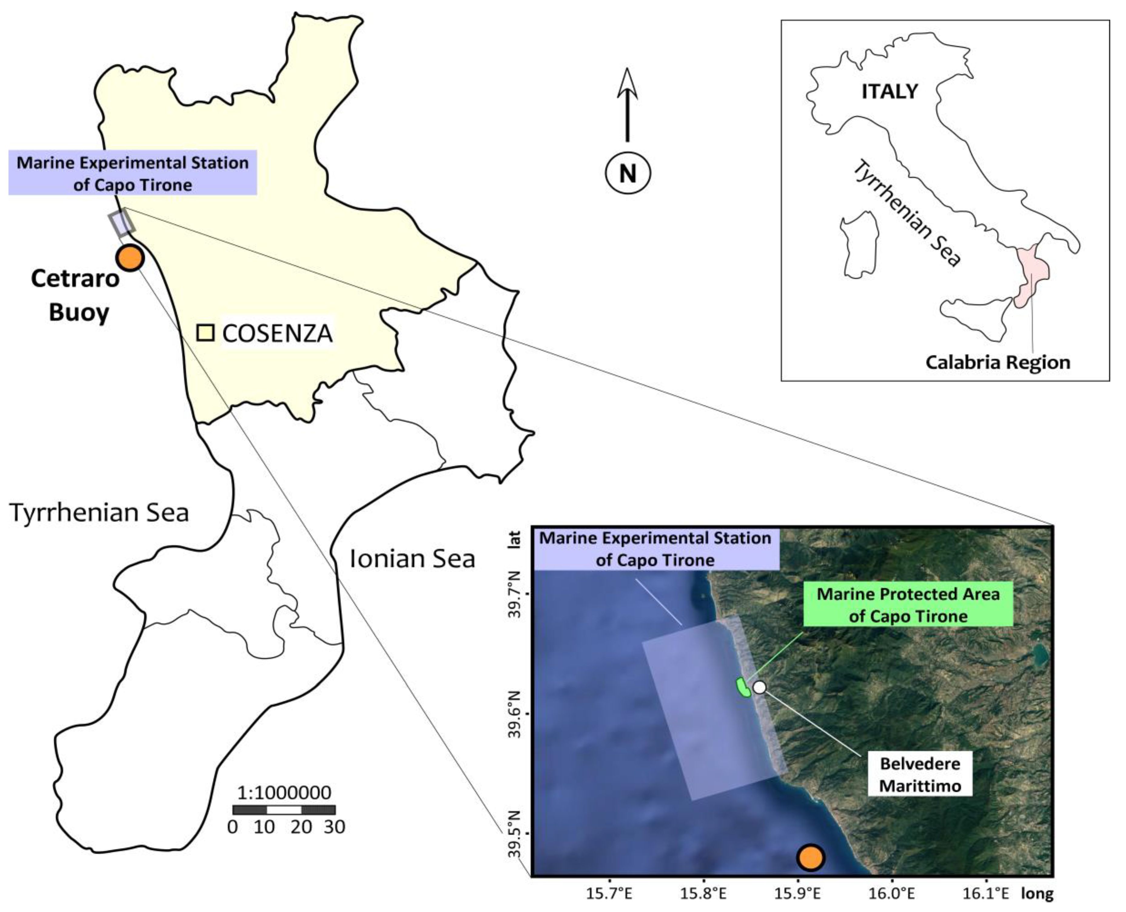
Calabria is characterized by a densely populated coastline, partly located in the Ionian Sea and partly in the Tyrrhenian Sea (Figure 1). The coastal areas of Calabria provide multiple services to the local population and economy, which is mostly based on fishing, tourism, and leisure activities [47]. In this paper, we focus on the Southern Tyrrhenian Coast belonging to the Province of Cosenza (Figure 1), which is significantly affected by erosion processes [47]. In the last decades, the shoreline experienced a significant retreat, threatening the coastal assets and the population [47,49]. The SCI_CT (IT9310033 Fondali di Capo Tirone) is located into the municipality of Belvedere Marittimo (Province of Cosenza, see Figure 1). The SCI_CT extends for 101 ha of marine surface into the MESCT. The seabed is characterized by the presence of Posidonia oceanica meadows, and it is classified as a 1120 * priority habitat for conservation under the Habitats Directive (Dir 92/43/CEE). Posidonia oceanica is a native seagrass of the Mediterranean Sea, providing multiple services to the environment and the ecosystem of the marine area, e.g., reducing wave power, erosion processes, and the bedload [50,51]. The prevailing wind directions range from 30° N to 150° N, whereas the coastline is affected by swell waves generated in the West Mediterranean Sea (incoming wave direction ranging from 210° N to 330° N). The mean spring tidal range at Capo Tirone is about 0.5 m; hence, the tidal currents and wave-current interactions are not significant. The storms affecting the area are mainly characterized by a ground-level trough located at the Genova Gulf that develops downwind of the Alps and moves southward. This pattern triggers intense western winds over the whole Tyrrhenian Sea, and it is named as a “typical Tyrrhenian storm” [52]. The local wind climate is strongly affected by the orography of the shoreline, since the Coastal Chain, extended up to the coastline, is high more than 1000 m above sea level (see Reference [47] for more details on the orography of the area).
The Marine Experimental Station of Capo Tirone
The MESCT (Figure 2) supports field monitoring surveys, research activities, and the development of mathematical models aimed at analyzing the local hydrodynamic and the erosion processes that have affected the shoreline in the last century [53,54]. The MECST has recently been equipped with a fixed buoy and a full weather station, fundamental for further monitoring activities concerning the local sea dynamic and the protection of the environment [47]. The actual plans aim to promote a sustainable management of the area, with particular reference to the SCI_CT, mainly based on nature-based solutions, such as the restoration of Posidonia oceanica meadows [45].
2.2. Dataset
Mathematical models can reproduce two-dimensional wave fields, simulating wave energy growth and dissipation, but much more attention needs to be paid to the lack and errors of the measured data [20,55]. Though few wave-gauging stations exist in the Southern Tyrrhenian Sea, the Cetraro buoy recorded a ten-year-long dataset. The Cetraro buoy is located about 10 km south from the MESCT (Figure 1), not providing a comprehensive spatial coverage of the region. Nevertheless, it can support the validation of the ERA5 and WAM models, which can be further used to explore and reproduce the wave climate of the region.
In this work we analyzed the following climate parameters: Significant Wave Height (SWH, approximating the average of the upper third of all individual wave heights derived from the 0th moment of the wave energy spectrum), Maximum Wave Height (HMAX), incoming Wave Direction (θ), Mean Wave Period (Tm, corresponding to the mean frequency of the spectrum), Peak Wave Period (Tp, corresponding to the maximum energy frequency), 10-m Wind Speed (W10), and incoming Wind Direction (θWind).
2.2.1. Cetraro Buoy Dataset
In this study, we used a ten-year-long wave climate dataset (from 27 February 1999 to 5 April 2008) based on the data collected by a Datawell Waverider buoy (Triaxys) located at Cetraro (39°27′12″ °N, 15°55′06″ °E, 100-m depth, see Figure 1) belonging to the Italian National Sea Wave Measurement Network (RON, see Reference [56]). This type of buoy is regularly adopted in coastal and marine engineering, and it can be considered standard industry equipment [57]. The Cetraro buoy collected significant wave height, period, and direction at intervals of 30 min. No wind data are available from this sensor.
2.2.2. ERA5 Hindcast
ERA5 is the latest global atmospheric hindcast reanalysis produced by ECMWF, following the FGGE, ERA-15, ERA-40, and ERA-Interim. ERA5 is based on a more recent version of the ECMWF Integrated Forecast System model (IFS 41r2), extending from the year 1950 to the present. The ERA5 dataset is open access at the Copernicus Climate Change Service [58,59]. The main improvements of ERA5 IFS 41r2 with respect to the former releases are (i) the output time step (one hour); (ii) the horizontal resolution (0.25° for climate parameters and 0.50° for wave parameters); (iii) the vertical resolution (137 vertical layers extending from the surface to 0.01 hPa); and (iv) the implementation of additional parameters (e.g., microphysics, convection, surface pressure, and ozone concentration), together with (v) the data assimilation technique. Compared to its predecessors, ERA5 improves the estimation of several climate variables, including rainfall and tropical convection [60], land surface temperature [61], downwelling solar radiation at the surface [62], and wind climate [63]. At present, ERA5 dataset is extended every three months. Since the analysis of a long dataset is fundamental to produce a reliable long-term trend, in this work, we used the whole 70-year-long dataset of ERA5, from January 1950 to December 2019, with a temporal resolution of six hours of SWH (m), Hmax (m), θ (deg), Tp (s), Tm (s), and W10 (m/s). Hereinafter, we refer to the ERA5 output point located west of Cetraro (39.5° N, 15.5° E, an almost 500-m depth).
2.2.3. WAM Model
With the aim to reproduce the storms that occurred in the last decade, when the gauged data at the Cetraro buoy were not available, we used the WAve Model hindcast (WAM), a high-resolution wave model developed by the Wave Model Development and Implementation Group [64]. The WAM simulations were performed for an eleven-year-long period between 2009 and 2019 integrated into the buoy dataset, and for the year 2006, compared to the gauged data. WAM solves the spectral equations to characterize the two-dimensional wave spectrum, forced by the ECMWF 10-m wind [65]. We used a two-grid nested configuration, with a horizontal resolution of 0.1° (lat/lon coverage: 28° N–45° N/5° W–24° E) and 0.05° (lat/lon coverage: 35° N–42° N/8° W–20° E) in both the north–south and east–west directions. As concerns the initial and dynamic boundary conditions, we used ECMWF wind data with a horizontal resolution of 0.25° (lat/lon coverage: 30° N–48° N/5° W–38° E) and a time step of six hours. We selected a spectrum of 25 frequency bands (frequency range 0.05–0.5 Hz) and 24 direction bands (15° of resolution). The output parameters are SWH, θ, and Tm, and the output time step is three hours for the whole period and one hour for the single storm analysis.
2.2.4. MIKE Hydrodynamical Model
MIKE 21-3 Coupled Model FM (hereinafter named as MIKE) is an integrated system based on a flexible mesh approach (i.e., unstructured grid) widely used to study ocean, coastal, and estuarine processes. MIKE solves the two- and three-dimensional incompressible Reynolds-averaged Navier–Stokes equations subject to the assumptions of Boussinesq and of hydrostatic pressure. Shallow water equations were solved through the approximate Riemann solver [66,67], and wave fields were described by the wave action conservation equations [68]. The wave boundary conditions were assigned by using a fully spectral formulation in the frequency domain (Jonswap spectrum, with the standard shape parameters). A detailed description of the model can be found in the scientific documentation compiled by the Danish Hydraulics Institute [69].
2.3. Methods
With the aim to assess the climatic trend and the interannual variability of the sea parameters at the MESCT (Section 3), we processed the ERA5 over a 70-yearl-ong period. The ERA5 performance was preliminary assessed by comparing the hindcast results to the observations at the Cetraro buoy within the period February 1999–April 2008. ERA5 data were stored every six hours across the computational domain (00:00, 06:00, 12:00, and 18:00 UTC). We compared the wave height, period, and direction through some standard statistics parameters and error metrics, i.e., mean, median, variance, 10th and 90th percentiles, standard deviation (SD), root mean square error (RMSE), mean absolute error (MAE), arithmetic mean value of the errors (Bias), Scatter Index (SI), and correlation coefficient (R2). The statistical significance of the annual and seasonal trends of SWH and Tm were calculated through the Mann–Kendall (MK) test [70,71], endorsed by the World Meteorological Organization for hydro-meteorological trend assessments [72], and widely used in wave climate analyses (see Reference [73] for an application in the Mediterranean Sea). The Sen’s slope estimator (SSE) was used to estimate the linear slope of the correlations. Finally, we performed the Innovative Trend Analysis (ITA) method [74]. The formulations of the statistic parameters and error metrics used in this study are described in Appendix A. Among the criteria adopted to remove the outliers [42], we neglected the data that showed a difference, computed with respect to the previous times, of 1.5 m, 5 s, and 30° for SWH, Tm, and θ, respectively. In reproducing the nearshore wave climate, we used MIKE forced with the wave climate computed by WAM. We validated the 2006 WAM dataset on buoy observations. Furthermore, we compared ERA5 and WAM over the period 2009–2019.
2.3.1. ERA5 Validation
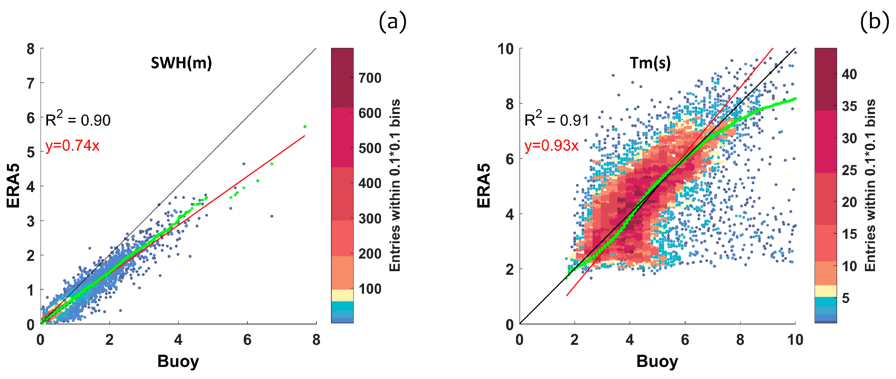
We compared SWH, Tm, and θ computed by ERA5 at Cetraro (Figure 3 and Table 1). Although a monitoring period of 1 to 2 years is deemed suitable to validate a wave model [20], we analyzed the whole buoy dataset (1999–2008).
Figure 3a shows the quantile–quantile SWH scatter plots between the ERA5 and Cetraro buoy dataset. ERA5 slightly overestimates SWH for small waves (<0.6 m) and underestimates SWH in strong sea conditions, consistent with the statistical parameters and error metrics reported in Table 1. The correlation between the ERA5 and buoy data can be expressed as a linear relationship with a 0.74 slope. This is the result of the widespread constraint of low-resolution models in reproducing the mesoscale of the surface wind climate with particular reference to the Mediterranean area, where the wave height increases with the model resolution, as shown by Reference [75]. The mean wave period comparison (Figure 3b and Table 1) showed a general underestimation of larger waves. Some differences were evidenced also in wave direction (Table 1), but they were limited to small waves and mainly caused by the effect of the local wind, which was not properly reproduced by ERA5.
2.3.2. WAM–ERA5 Difference
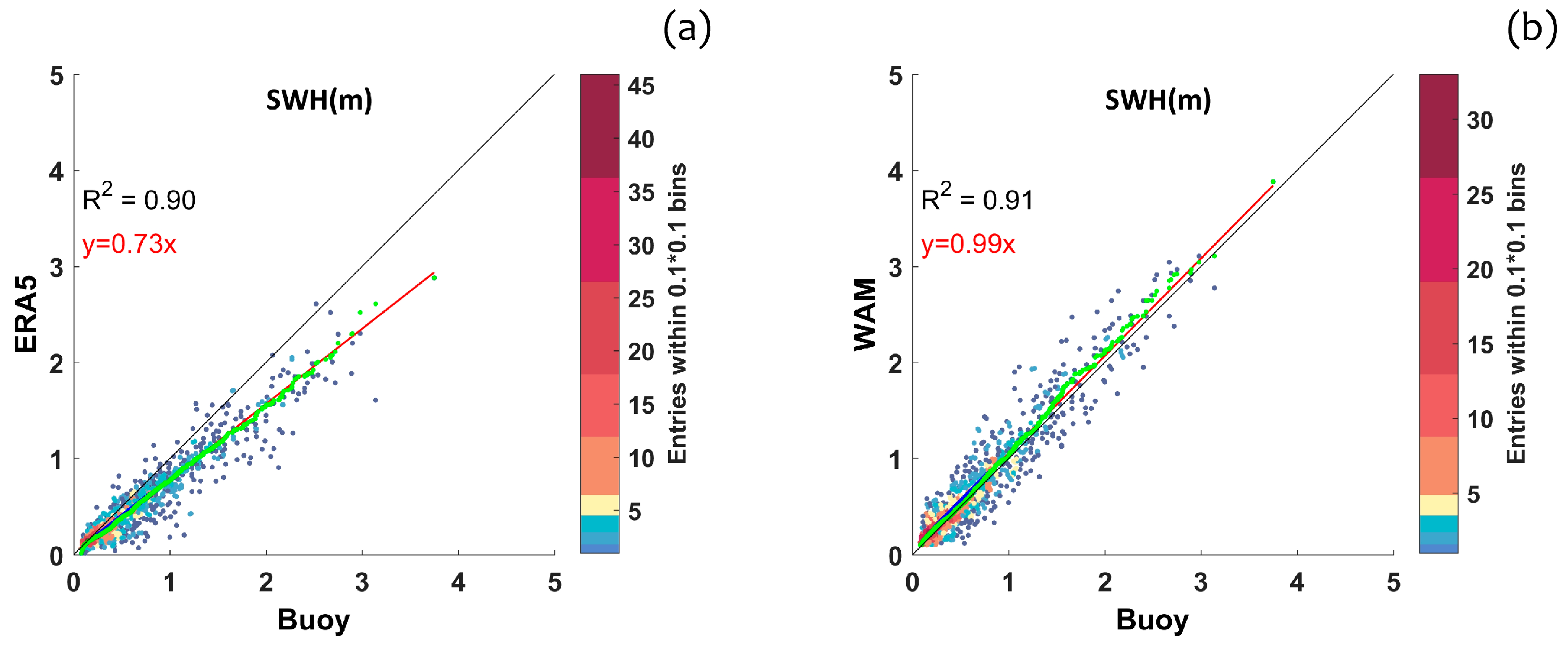
SWH and Tm comparisons between ERA5 and WAM hindcast provided a linear relationship with slopes of almost 0.9 and 1.0, respectively (Figure 4 and Table 2). As the slope of the SWH correlation was slightly higher if compared to the correlation between ERA5 and buoy data, we argue that WAM underestimates wave heights less. A possible explanation is the finer resolution of the grid of the WAM model (5 km), consistent with Reference [75]. Similar results were obtained for Tm and θ (Table 2).
3. Results and Discussion
With the aim to describe the wave climate at the MESCT, we processed the ERA5 reanalysis dataset from 1950 to 2019, focusing on the wave climate (Section 3.1), its seasonal variability (Section 3.1.1), possible trends (Section 3.1.2), and the inshore wave characteristics (Section 3.2).
3.1. Off-Shore Wind and Wave Climatology
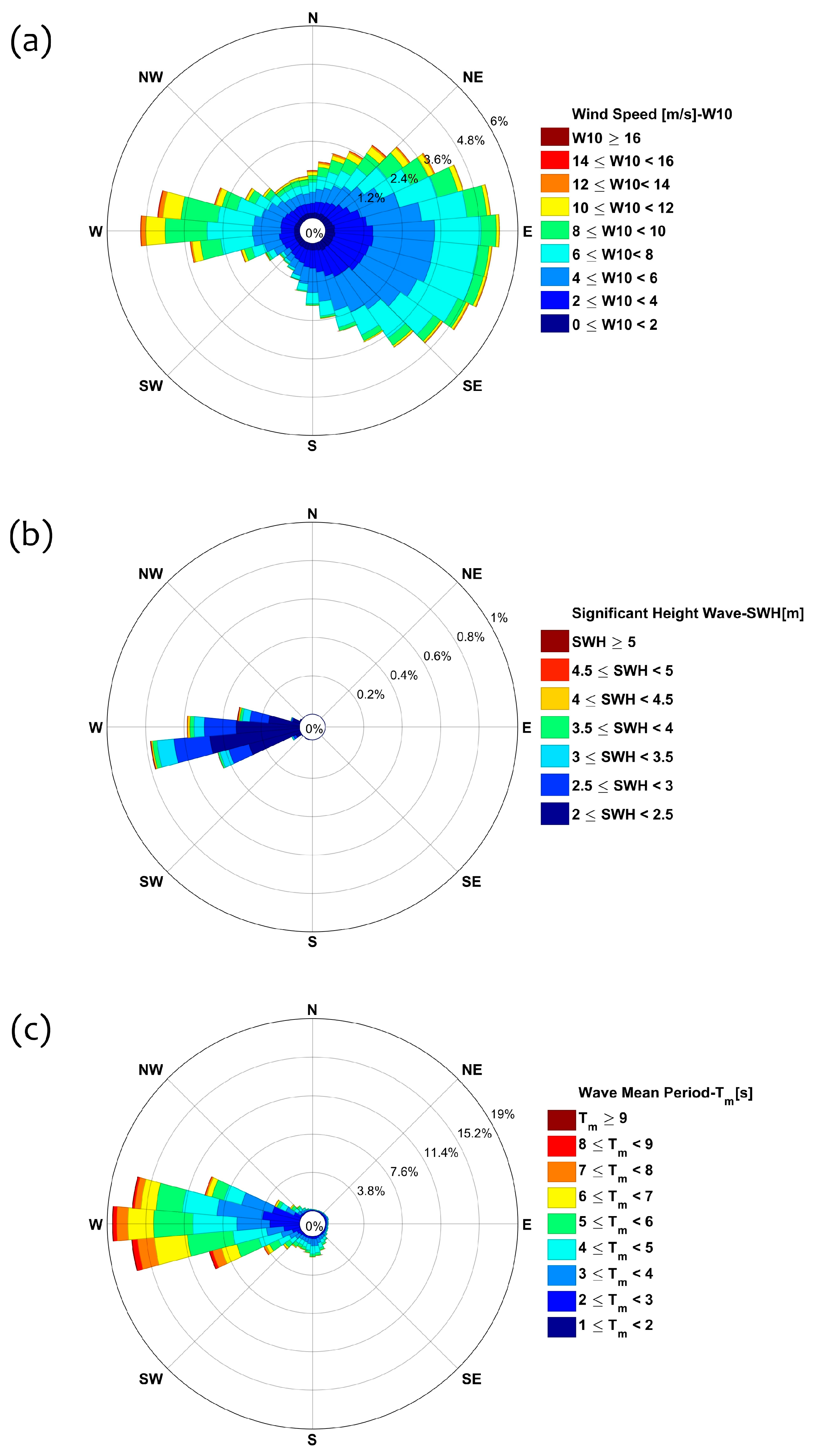
Wind and wave roses in Figure 6 illustrate the frequency and relative percentiles of W10, SWH, and Tm of wind and waves coming from a certain direction at the MESCT. The analysis of the ERA5 dataset provided a predominant western mean wave direction θ (Figure 6b,c), according to other studies performed in the Southern Tyrrhenian Sea [42,76]. Wave fields are driven by the Mistral-Etesian and Scirocco-Libeccio wind regimes, as highlighted in Figure 6a. However, due to the null fetch in the northern and eastern directions at the shoreline belonging to the MESCT (i.e., from 345° N to 135° N, see Figure 1), 50% of the waves of SWH > 2 m corresponded to the WNW direction (270° N–315° N) and 50% to the WSW (225° N–270° N).
3.1.1. Seasonal Variability
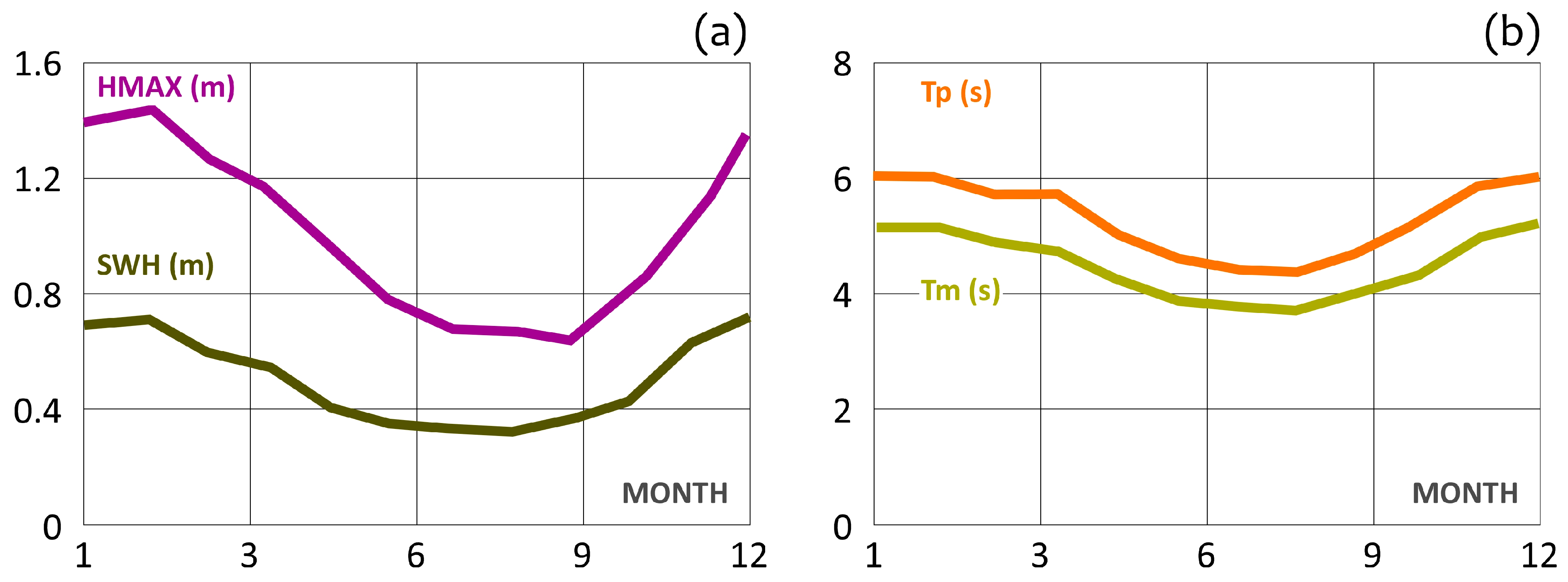
The wave climate in the Southern Tyrrhenian Sea shows a significant seasonality [42], characterized by a relatively calm sea in the hot season (from March to August) and strong sea triggered by the Mistral and Libeccio winds during the cold season (from September to February). Figure 7 shows the monthly average of the SWH and HMAX (a) and Tm and Tp (b) at the MESCT, computed on the basis of the 70-year-long ERA5 dataset.
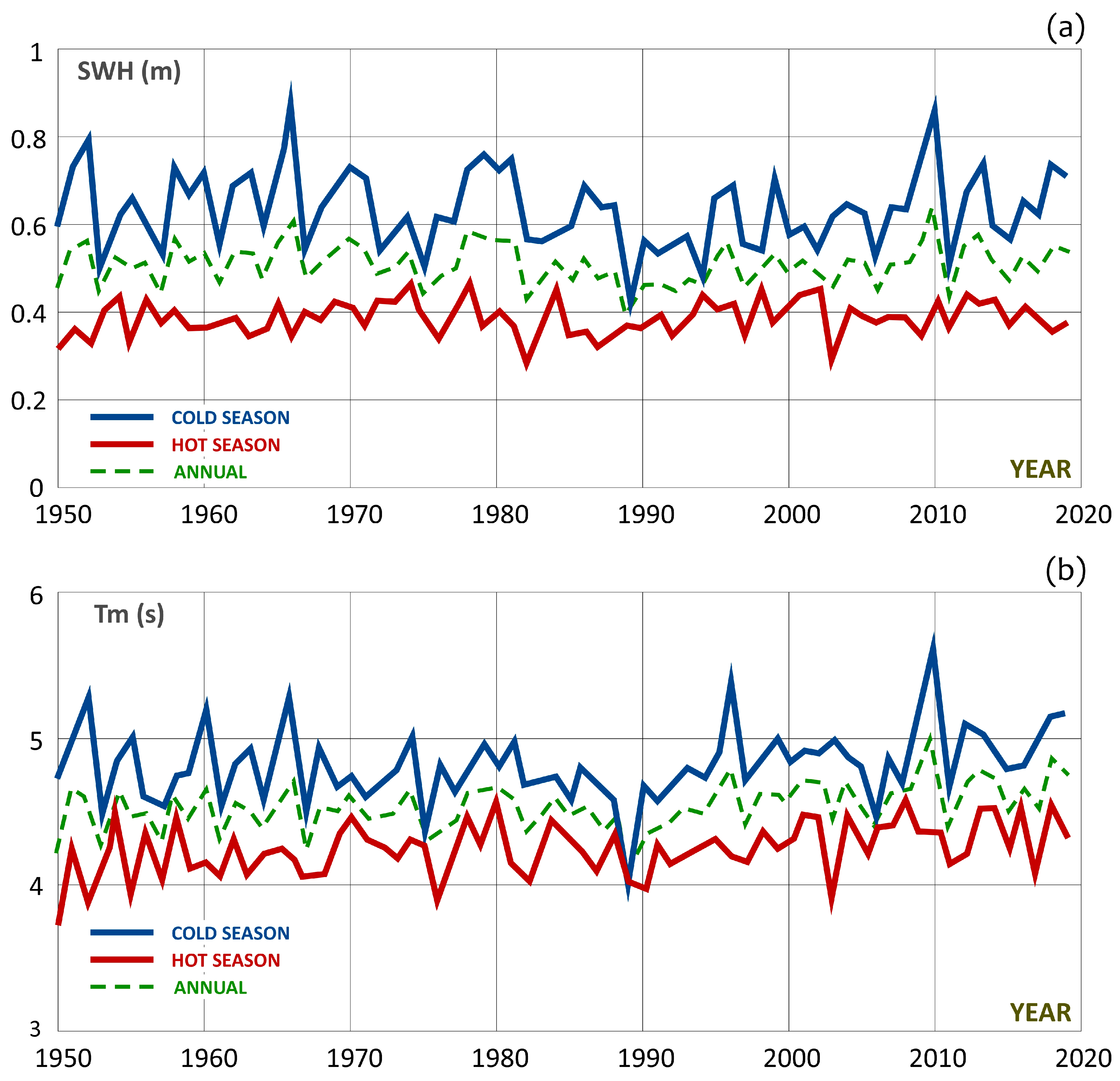
Figure 8 compares the seasonal mean (i.e., hot and cold seasons) of the SWH (a) and Tm (b) to the annual mean for each year of the ERA5 dataset. Table 3 and Table 4 report some statistical parameters referred to the four seasons defined according to the World Meteorological Society standards for the Northern Hemisphere: winter from December to February (DJF), spring from March to May (MAM), summer from June to August (JJA), and autumn from September to November (SON). The MESCT area experiences a significant difference between the four seasons: the minimum wave forcing occurs in the summer, whereas in the fall and in spring we notice a wave climate similar to the annual mean. Higher and longer waves characterize the cold season in almost all the years within the period 1950–2019.
3.1.2. Trend Analysis
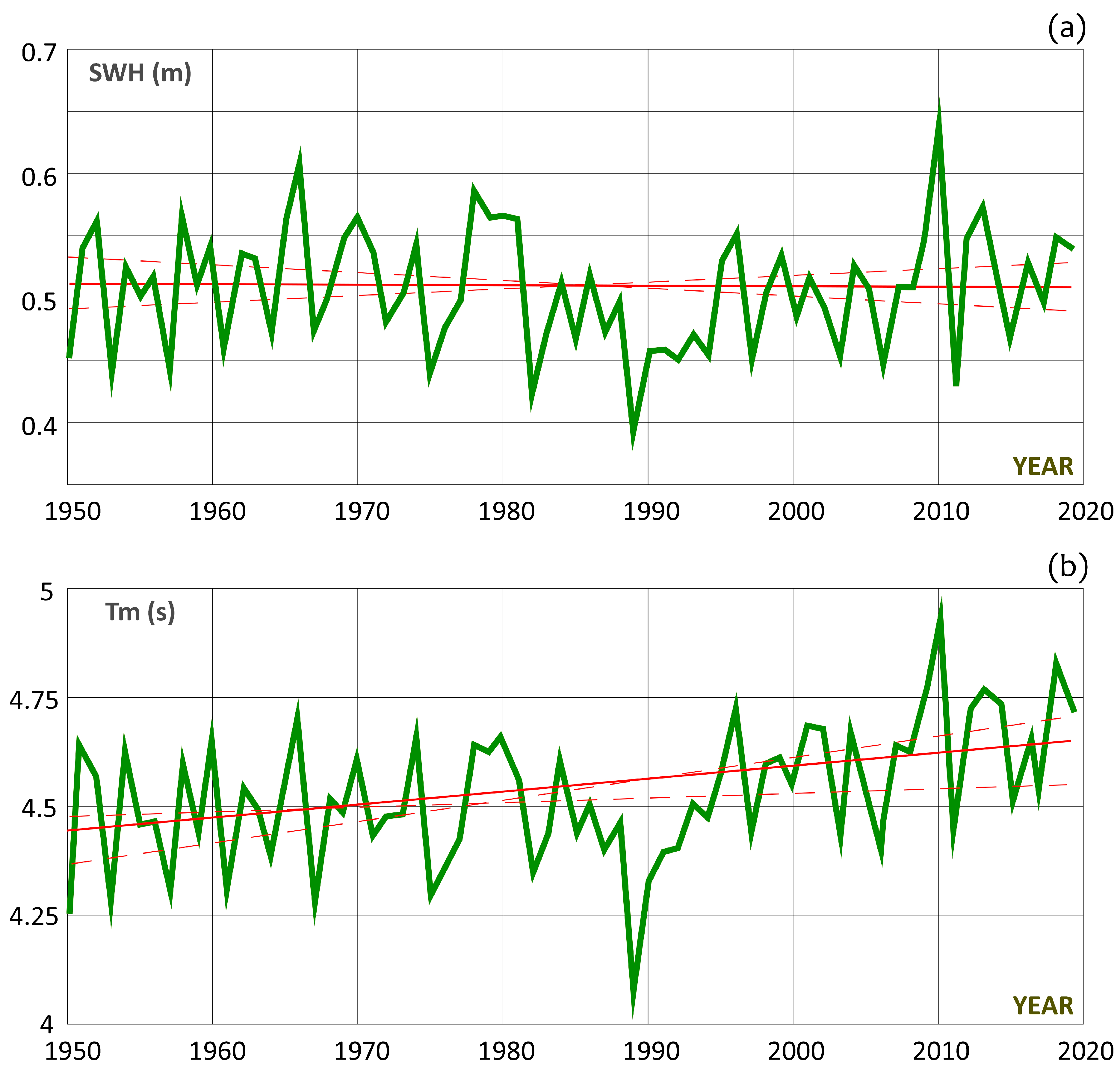
Figure 9 and Table 5 and Table 6 report the annual trend of the wave climate (SWH and Tm) at the MESCT based on ERA5 reanalysis dataset. The possible monotonic trend was investigated by computing the nonparametric MK test and the SSE estimator [77]. Despite our findings showing a large annual variability of the SWH and Tm, the results allowed to infer a slight positive trend for the mean wave period only (significance at 95%), according to Reference [42]. The MK test was further used to identify the possible monthly and seasonal trends [78], where the significance levels of the test (90%, 95%, and 98%) were highlighted with “S”, “SS”, and “SSS”, respectively (Table 5 and Table 6). Some months show an increasing trend in the wave period but mostly not significantly. As concerns the seasonal analysis, the spring, fall, and summer showed an increasing trend of Tm significant at 95%, 90%, and 98%, respectively, whereas the SWH exhibited non-significant trends. In the winter, we observed for both the SWH and Tm non-significant trends. The Tp and HMAX (not shown) showed similar trends.
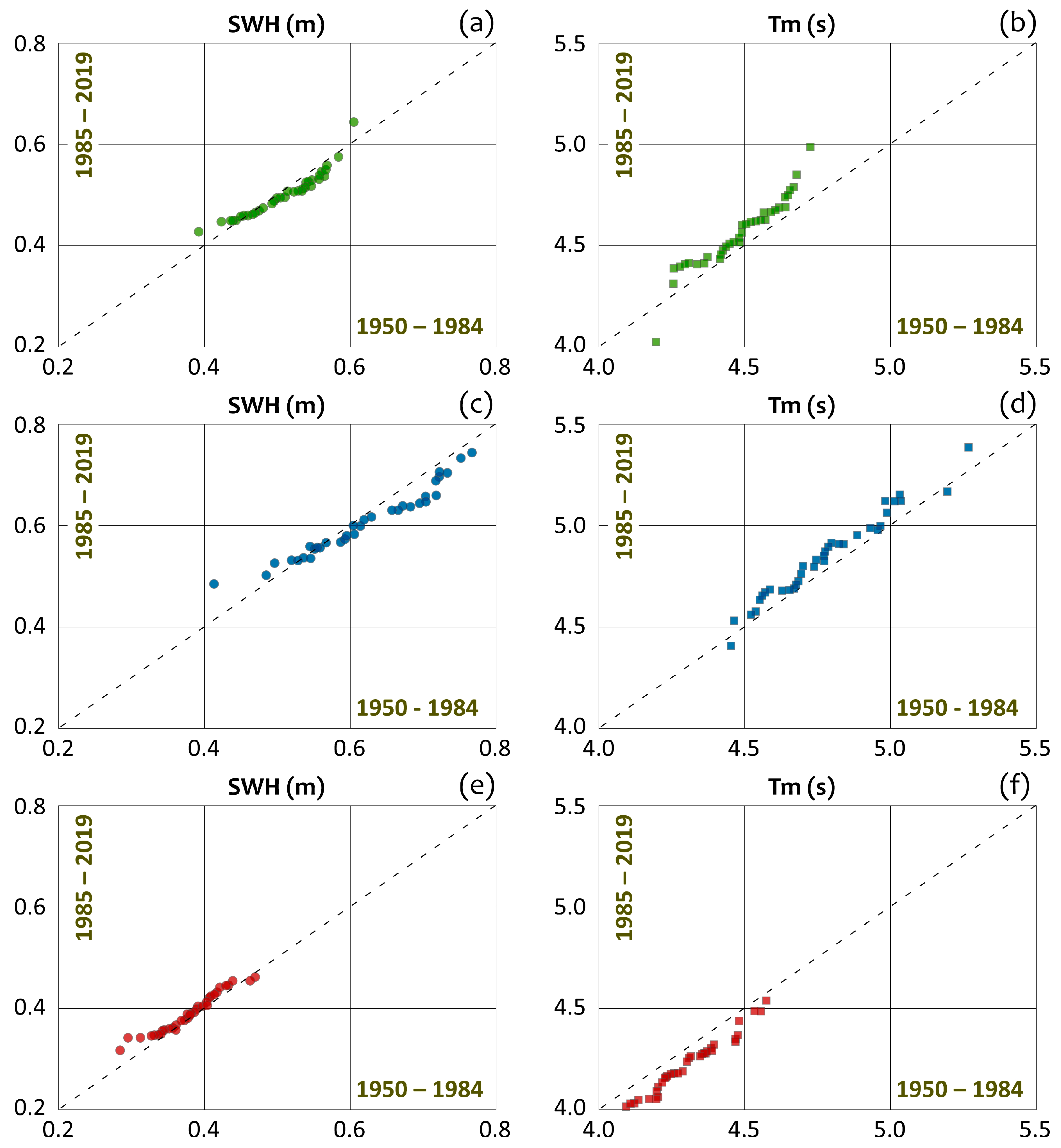
Figure 10 illustrates the Innovative Trend Analysis (ITA), widely applied in hydrology [74,79,80]. We compared two ERA5 sub-datasets (i.e., 1950–1984, x-axis, and 1985–2019, y-axis) sorted in ascending order. We investigated the average annual (green), cold season (blue), and hot season (red) trends for SWH and Tm. The MK test trends were confirmed through the ITA.
3.2. Nearshore Wave Analysis
We investigated how the nearshore wave climate is affected by the complex morphology of the coastline to gain further insights into the MESCT variability of the sea state. Numerical simulations were carried out using the MIKE model, which reproduces growth, decay, and transformation of wind sea and swell waves [69]. The sensitivity analysis of the spatial and temporal resolutions, as well as the boundaries of the model domain, were carried out to identify its optimum resolution, extent, performance, and time consumption. The model domain included all the MESCT area 4 km north of Diamante, 4 km south of Cape Bonifati, and 6 km seaward (Figure 10b). The computational mesh consisted of about 1200 nodes and 2500 triangular elements of characteristic sizes (side-length) of almost 600 m. Smaller elements (200 m) described the SCI_CT area and the two sections where we investigated the suitability of the deployment of a new monitoring buoy. MIKE was forced by imposing (i) SWH at the seaward boundary section (SBS) computed by the WAM every 60 min at the output sections (yellow bullets), (ii) lateral conditions at the two lateral boundary sections (LBS), and land condition at the coastal boundary section (CBS). A uniform wind field computed by ERA5 was assigned within the whole domain.
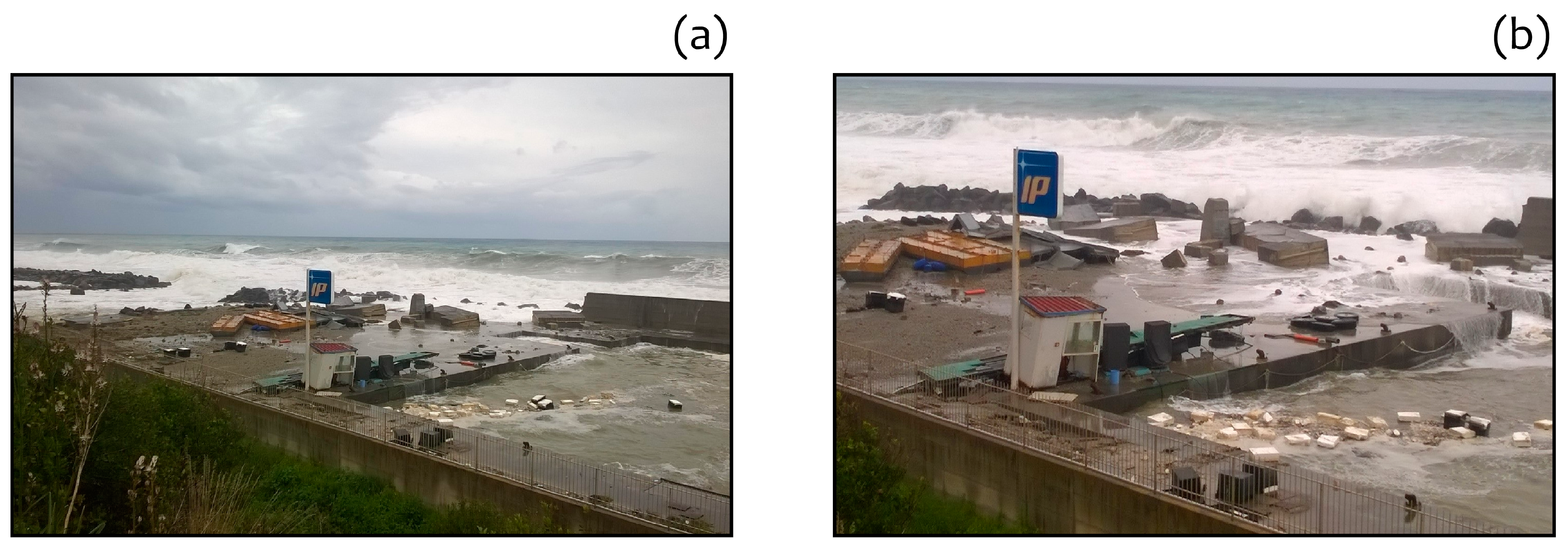
We first reproduced a storm that occurred on 21 March 2018, which struck all the Southern Tyrrhenian coast, causing multiple devastating floods (see Figure 11 and Figure 12 and Reference [81] for more details). The storm was characterized by intense southwestern winds triggered by a ground-level trough located over the Central Tyrrhenian Sea. Figure 11 illustrates the SWH computed at the full power of the storm (21 March, 09 UTC) in the whole domain of the WAM (Figure 11a), the domain of MIKE (Figure 11b), and the nearshore bathymetry (Figure 11c).
The results evidenced a large variability in the SWH within the Southern Tyrrhenian Sea, with higher waves approaching the coast (Figure 11a). Nearshore simulations performed by MIKE showed a further variability of the wave climate within the study area, which was affected by the local bathymetry. In general, the SWH were larger in higher water depths and exposure. Furthermore, Cape Diamante located north of the MESCT could cause regions of sheltering and lower wave energy with respect to the southern area. In addition, subtidal sandbanks and Posidonia oceanica meadows caused regions of focusing and defocusing via refraction. This was particularly evident in the vicinity of the shoreline.
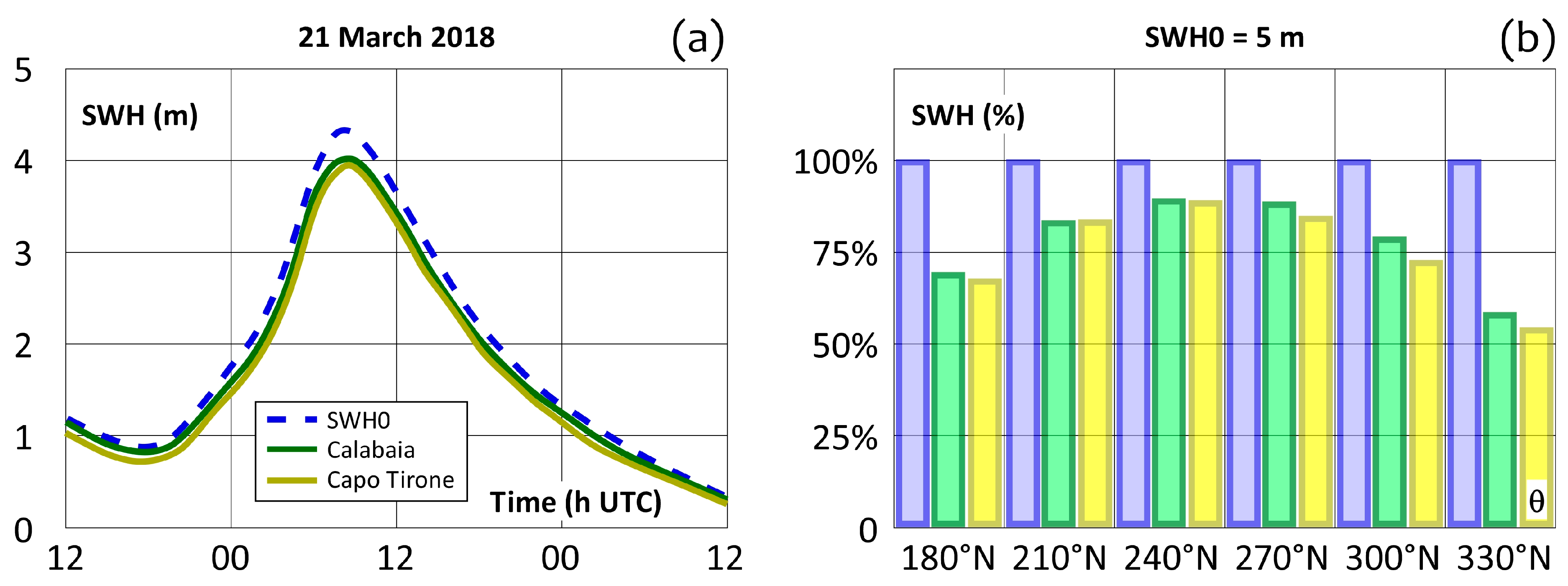
To identify the optimal location to deploy a monitoring buoy, we compared the SWH computed at two sections eligible for buoy deployment to the offshore SWH boundary conditions (namely, Calabaia and Capo Tirone, Figure 11c). As concerns the event of 21 March 2008 (Figure 13a), Calabaia showed a SWH slightly less affected by the local morphology due to the lower seabed elevation. With the aim to draw a general trend, we systematically computed the SWH damping from the SBS (i.e., SWH0) in the same two sections and for wave directions θ ranging from 180° N to 330° N and a constant SWH0 ranging from 1 to 8 m (Figure 13b reports the example of SWH0 = 5 m). The results confirmed a higher SWH for the Calabaia location for almost all the θ. As a note, this was only a preliminary assessment, which should be followed by a thorough study (e.g., a ray-tracing analysis) to confirm the results.
4. Conclusions
This work provided insights into the wave climate at the Marine Experimental Station of Capo Tirone (MESCT), located in the Southern Tyrrhenian Sea (Italy). A statistical trend analysis of the significant wave height and period was performed with a 70-year-long wave hindcast within the period 1950–2019. We analyzed the ERA5 reanalysis dataset validated at the Cetraro buoy within the period 1999–2008. Furthermore, we investigated the local spatial variability of the wave climate by means of the WAM and MIKE high-resolution models. Specifically:
- -
- beside a general underestimation of wave height and period, ERA5 showed satisfactory results, accurately estimating the wave climate in the Southern Tyrrhenian Sea. Typical values of the average monthly bias were −0.15 m (wave height) and −0.13 s (wave period), with correlation coefficients R2 of about 0.9. The WAM model evidenced a smaller negative bias than ERA5, compared to the buoy data, proving to be a fundamental tool to counterbalance the recent lack of data at the Cetraro buoy;
- -
- the 70-year long ERA5 dataset showed that the offshore wave climate at Capo Tirone was characterized by a mean significant wave height of about 0.5 m. The mean maximum wave height and peak period exceeded 1.2 m and 6 s, respectively, corresponding to the major storms occurring in the winter. Furthermore, the results evidenced a clear seasonality for both the wave height and wave period and a strong interannual variability;
- -
- -
- nearshore wave modeling provided instructive insight into the spatial variability of the wave climate. The location in front of Calabaia is considered most suitable for buoy deployment and for further wave climate monitoring at the Marine Experimental Station of Capo Tirone.
The data presented in this paper are expected to provide insights on the role of the wave climate in coastal processes of the Southern Tyrrhenian Coast. These data can be used for multiple research purposes, such as the long-term variability of wind sea and swell wave climates and nearshore sediment transport, supporting the assessment of the effects of coastal hazards related to climate change and extreme wave actions. Although the interactions between the waves and shoreline currents were beyond the aim of this work, it is worth investigating the possible results in higher waves during strong storms, improving the prediction accuracy [82]. Furthermore, the possible effect of watercourse discharge on the wave climate is an important topic to assess, as river flows can affect the interactions between waves and shorelines currents and salt intrusion [20,83,84].
Lastly, our findings highlighted the urgent need to conduct extensive high-resolution bathymetric surveys on the marine protected area of Capo Tirone and to deploy a buoy to monitor the local state of the sea. These works will pertain to the Marine Experimental Station of Capo Tirone, which is set to become a crucial hub for supporting the sustainable development of the Southern Tyrrhenian Coast belonging to the Province of Cosenza.
Author Contributions
T.L.F.: conceptualization, methodology, investigation, data curation, validation, visualization, and writing—review and editing; R.A.M.: conceptualization, methodology, investigation, validation, visualization, writing—original draft, and writing—review and editing; S.S.: conceptualization, methodology, investigation, data curation, validation, and visualization; and M.M.: conceptualization, methodology, validation, visualization, writing—review and editing, supervision, funding acquisition, and project administration. All authors have read and agreed to the published version of the manuscript.
Funding
This work was partially funded by the Italian Ministry of University and Research (MIUR) through Project PON-AIM “Attraction and International Mobility”, Action I.2, CUP: H24I19000360005.
Institutional Review Board Statement
Not applicable.
Informed Consent Statement
Not applicable.
Data Availability Statement
All the data used in the paper are available by contacting the corresponding author.
Conflicts of Interest
The authors declare no conflict of interest. The funders had no role in the design of the study; in the collection, analyses, or interpretation of the data, in the writing of the manuscript; or in the decision to publish the results.
Appendix A
The error metrics used in this paper are (A1) the root mean square error (RMSE), (A2) the mean absolute error (MAE), (A3) the arithmetic mean value of the errors (Bias), (A4) the Scatter Index (SI), and (A5) the correlation coefficient (R2).
In all the formulations, ei is the estimation of a certain variable (ERA5 and WAM), oi represents the in situ observations (buoy data) and n is the amount of data.
The Mann–Kendall test (MK) (A6) has been used to identify possible monotonic trends:
where xj and xk are the annual means j and k (with j = k + 1), and
If n < 10, the absolute value of MK is compared directly to the theoretical distribution derived by Mann and Kendall (Gilbert, 1987). If n > 10, the test provides a normal distribution with the mean (μ = 0) (Helsel and Hirsch 1992) and variance VAR (MK) defined by Equation (A8).
where qj is defined as the tied group, and tj the number of observations in the jth group. The possible significant trend has been identified by using the Z value (A9). Specifically, a positive (negative) value of Z indicates an increasing (decreasing) trend:
In Table 5 and Table 6, we calculated Z at different significance levels, i.e., 90%, 95%, and 99% (two tailed test).
We further used the Sen’s nonparametric method to estimate the linear slope of a possible trend. For given time series data Xi = x1, x2, …, xn, the Sen’s slope equation is:
where A is the slope, and B is the intercept. The parameter A is estimated by computing the slopes of all pairs of data (A11):
where the total number N of Ai is defined as (A12):
where n is the total number of xj of the dataset. The Sen’s slope Amed (A13) is defined as the median of the N ranked values of Ai:
A positive value of Amed represents an increasing trend and vice versa.
Appendix B
Table A1 reports the acronyms we used in the manuscript.

Table A1.
List of acronyms used in this work (alphabetical order).
| Bias | Arithmetic Mean Value of the Errors |
| CBS | Coastal Boundary Section |
| DJF | Winter (December–February) |
| ERA5 | ECMWF Reanalysis v5 |
| ECMWF | European Centre for Medium-Range Weather Forecasts |
| HMAX | Maximum Wave Height |
| IFS41r2 | ECMWF Integrated Forecast System model |
| ITA | Innovative Trend Analysis |
| JJA | Summer (June–August) |
| LBS | Lateral Boundary Section |
| MAE | Mean Absolute Error |
| MAM | Spring (March–May) |
| MESCT | Marine Experimental Station of Capo Tirone |
| MIKE | MIKE 21-3 Coupled Model FM |
| MK | Mann-Kendall test |
| R2 | Correlation Coefficient |
| RMSE | Root Mean Square Error |
| RON | Italian National Sea Wave Measurement Network |
| SBS | Seaward Boundary Section |
| SCI_CT | Marine Protected Area of Capo Tirone |
| SD | Standard Deviation |
| SI | Scatter Index |
| SON | Autumn (September–November) |
| SSE | Sen’s Slope Estimator |
| SWH | Significant Wave Height |
| Tm | Mean Wave Period |
| Tp | Peak Wave Period |
| WAM | WAve Model |
| W10 | 10 m Wind Speed |
| θ | Wave Direction |
| θWind | Wind Direction |
References
- OECD. Marine Protected Areas: Economics, Management and Effective Policy Mixes; OECD Publishing: Paris, France, 2017. [Google Scholar] [CrossRef]
- Roumasset, J.K.; Brooks, K. Valuing Indirect Ecosystem Services: The Case of Tropical Watersheds. Environ. Dev. Econ. 2002, 7, 701–714. [Google Scholar] [CrossRef] [Green Version]
- Jorve, J.; Kordas, R.; Anderson, K.; Nelson, J.; Picard, M.; Harley, C. Climate Change: Coastal Marine Ecosystems. Encycl. Nat. Resour. Air 2014. [Google Scholar] [CrossRef]
- Costanza, R.; d’Arge, R.; de Groot, R.; Farber, S.; Brasso, M.; Hannon, B.; Limburg, K.; Naeem, S.; O’Neill, R.V.; Paruelo, J.; et al. The value of the world’s ecosystem services and natural capital. Nature 1997, 387, 253–260. [Google Scholar] [CrossRef]
- Hoegh-Guldberg, O.; Bruno, J.F. The impact of climate change on the world’s marine ecosystems. Science 2010, 328, 1523–1528. [Google Scholar] [CrossRef] [PubMed]
- Hoozemans, F.M.J.; Marchand, M.; Pennekamp, H.A. A Global Vulnerability Analysis: Vulnerability Assessment for Population, Coastal Wetlands and Rise Production on a Global Scale, 2nd ed.; Delft Hydraulics: Delft, The Netherlands, 1993. [Google Scholar]
- Tol, R.S.J. The double trade-off between adaptation and mitigation for sea level rise: An application of FUND. Mitig. Adapt. Strateg. Glob. Chang. 2007, 5, 741–753. [Google Scholar] [CrossRef] [Green Version]
- Vafeidis, A.T.; Nicholls, R.J.; McFadden, L.; Tol, R.S.J.; Spencer, T.; Grashoff, P.S.; Boot, G.; Klein, R.J.T. A new global coastal database for impact and vulnerability analysis to sea-level rise. J. Coast. Resour. 2008, 24, 917–924. [Google Scholar] [CrossRef]
- Nicholls, R.J.; Marinova, N.; Lowe, J.A.; Brown, S.; Vellinga, P.; de Gusmão, D.; Hinkel, J.; Tol, R.S.J. Sea-level rise and its possible impacts given a ‘beyond 4 degrees C world’ in the twenty-first century. Philos. Trans. R. Soc. 2011, 369, 161–181. [Google Scholar] [CrossRef] [Green Version]
- Mel, R. Exploring the partial use of the Mo. S.E. system as effective adaptation to rising flood frequency of Venice. Nat. Hazards Earth Syst. Sci. 2021, 21, 3629–3644. [Google Scholar] [CrossRef]
- Mel, R.; Carniello, L.; Viero, D.P.; Defina, A.; D’Alpaos, L. The first operations of Mo. S.E. system to prevent the flooding of Venice: Insights on the hydrodynamics of a regulated lagoon. Estuar. Coast. Shelf Sci. 2021, 261, 107547. [Google Scholar] [CrossRef]
- Jena, B.K.; Rajkumar, J.; Avula, A.; Jossia, K.; Murthy, M. Simulated wave climate and variability over the North Indian Ocean. Curr. Sci. 2020, 118, 11. [Google Scholar] [CrossRef]
- Lee, Y.H.; Shindell, D.T.; Faluvegi, G.; Pinder, R.W. Potential impact of a US climate policy and air quality regulations on future air quality and climate change. Atmos. Chem. Phys. 2016, 16, 5323–5342. [Google Scholar] [CrossRef] [Green Version]
- Giorgi, F.; Bi, X.; Pal, J. Mean, interannual variability and trends in a regional climate change experiment over Europe. II: Climate change scenarios (2071–2100). Clim. Dyn. 2004, 23, 839–858. [Google Scholar] [CrossRef]
- Vecchi, G.A.; Wittemberg, A.T. El Niño and our future climate: Where do we stand? Wiley Interdiscip. Rev. Clim. Chang. 2010, 1, 260–270. [Google Scholar] [CrossRef]
- Pasaric, M.; Orlic, M. Meteorological forcing of the Adriatic: Present vs. projected climate conditions. Geofizika 2004, 21, 69–87. [Google Scholar]
- Conte, D.; Lionello, P. Storm surge distribution along the Mediterranean coast: Characteristics and evolution. Procedia-Soc. Behav. Sci. 2014, 120, 110–115. [Google Scholar] [CrossRef] [Green Version]
- Bellafiore, D.; Bucchignani, E.; Gualdi, S.; Carniel, S.; Djurdjevic, V.; Umgiesser, G. Assessment of meteorological climate models as inputs for coastal studies. Ocean Dyn. 2012, 62, 555–568. [Google Scholar] [CrossRef]
- Bolanos-Sanchez, R.; Sanchez-Arcilla, A.; Cateura, J. Evaluation of two atmospheric models for wind-wave modelling in the NW Mediterranean. J. Mar. Syst. 2007, 65, 336–353. [Google Scholar] [CrossRef]
- Yang, Z.; García-Medina, G.; Wu, W.C.; Wang, T.; Ruby Leung, L.; Castrucci, L.; Mauger, G. Modeling analysis of the swell and wind-sea climate in the Salish Sea. Estuar. Coast. Shelf Sci. 2019, 224, 289–300. [Google Scholar] [CrossRef]
- Gippius, F.; Myslenkov, S.A. Black Sea’s wind wave climate with a focus on coastal regions. Ocean. Eng. 2020, 218, 108199. [Google Scholar] [CrossRef]
- Booij, N.; Ris, R.C.; Holthuijsen, L.H. A third-generation wave model for coastal regions. Model description and validation. J. Geophys. Res.-Ocean. 1999, 104, 7649–7666. [Google Scholar] [CrossRef] [Green Version]
- Campos, R.M.; Alves, J.H.G.M.; Soares, C.G.; Guimaraes, L.G.; Parente, C.E. Extreme wind-wave modeling and analysis in the south Atlantic Ocean. Ocean Model. 2018, 124, 75–93. [Google Scholar] [CrossRef]
- Mulligan, R.P.; Bowen, A.J.; Hay, A.E.; van der Westhuysen, A.J.; Battjes, J.A. Whitecapping and wave field evolution in a coastal bay. J. Geophys. Res.-Ocean. 2008, 113. [Google Scholar] [CrossRef] [Green Version]
- Gedan, K.B.; Silliman, B.R.; Bertness, M.D. Centuries of human-driven change in saltmarsh ecosystems. Annu. Rev. Mar. Sci. 2009, 1, 117–141. [Google Scholar] [CrossRef] [PubMed] [Green Version]
- Liquete, C.; Zulian, G.; Delgado, I.; Stips, A.; Maes, J. Assessment of coastal protection as an ecosystem service in Europe. Ecol. Indic. 2013, 30, 205–217. [Google Scholar] [CrossRef] [Green Version]
- Mel, R.; Sterl, A.; Lionello, P. High resolution climate projection of storm surge at the Venetian coast. Nat. Hazards Earth Syst. Sci. 2013, 13, 1135–1142. [Google Scholar] [CrossRef] [Green Version]
- Nayak, S.; Bhaskaran, P.K.; Venkatesan, R.; Dasgupta, S. Modulation of local windwaves at Kalpakkam from remote forcing effects of Southern Ocean swells. Ocean. Eng. 2013, 64, 23–35. [Google Scholar] [CrossRef]
- Mel, R.; Lionello, P. Storm surge ensemble prediction for the city of Venice. Weather Forecast. 2014, 29, 1044–1057. [Google Scholar] [CrossRef]
- Bendoni, M.; Mel, R.; Solari, L.; Lanzoni, S.; Francalanci, S.; Oumeraci, H. Insights into lateral marsh retreat mechanism through localized field measurements. Water Resour. Res. 2016, 52, 1446–1464. [Google Scholar] [CrossRef] [Green Version]
- Albarakati, A.M.A.; Aboobacker, V.M. Wave transformation in the nearshore waters of Jeddah, west coast of Saudi Arabia. Ocean Eng. 2018, 163, 599–608. [Google Scholar] [CrossRef]
- Finotello, A.; Marani, M.; Carniello, L.; Pivato, M.; Roner, M.; Tommasini, L.; D’alpaos, A. Control of wind-wave power on morphological shape of salt marsh margins. Water Sci. Eng. 2020, 13, 45–56. [Google Scholar] [CrossRef]
- Mel, R.; Carniello, L.; D’Alpaos, L. How long the Mo. S.E. barriers will be effective in protecting all the urban settlements in the Venice lagoon? The wind setup constraint. Coast. Eng. 2021, 168, 103923. [Google Scholar] [CrossRef]
- Scarascia, L.; Lionello, P. Global and regional factors contributing to the past and future sea level rise in the northern Adriatic Sea. Glob. Planet. Chang. 2013, 106, 51–63. [Google Scholar] [CrossRef]
- Pranzini, E.; Wetzel, A.; Williams, A. Aspects of coastal erosion and protection in Europe. J. Coast. Conserv. 2015, 19, 445–459. [Google Scholar] [CrossRef]
- Pytharoulis, I.; Craig, G.C.; Ballard, S.P. The hurricane-like Mediterranean cyclone of January 1995. Meteorol. Appl. 2000, 7, 261–279. [Google Scholar] [CrossRef]
- Davolio, S.; Miglietta, M.M.; Moscatello, A.; Pacifico, F.; Buzzi, A.; Rotunno, R. Numerical forecast and analysis of a tropical-like cyclone in the Ionian Sea. Nat. Hazard. Earth Syst. Sci. 2009, 9, 551–562. [Google Scholar] [CrossRef] [Green Version]
- Miglietta, M.M.; Laviola, S.; Malvaldi, A.; Conte, D.; Levizzani, V.; Price, C. Analysis of tropical-like cyclones over the Mediterranean Sea through a combined modeling and satellite approach. Geophys. Res. Lett. 2013, 40, 2400–2405. [Google Scholar] [CrossRef]
- Lionello, P.; Sanna, A. Mediterranean wave climate variability and its links with NAO and Indian Monsoon. Clim. Dyn. 2005, 25, 611–623. [Google Scholar] [CrossRef]
- Galanis, G.; Hayes, D.; Zodiatis, G.; Chu, P.C.; Kuo, Y.H.; Kallos, G. Wave height characteristics in the Mediterranean Sea by means of numerical modeling, satellite data, statistical and geometrical techniques. Mar. Geophys. Res. 2012, 33, 1–15. [Google Scholar] [CrossRef] [Green Version]
- Pomaro, A.; Cavaleri, L.; Lionello, P. Climatology and trends of the Adriatic Sea wind waves: Analysis of a 37-year long instrumental data set. Int. J. Climatol. 2017, 37, 4237–4250. [Google Scholar] [CrossRef]
- Caloiero, T.; Aristodemo, F.; Algieri-Ferraro, D. Trend analysis of significant wave height and energy period in southern Italy. Theor. Appl. Climatol. 2019, 138, 917–930. [Google Scholar] [CrossRef]
- Caloiero, T.; Aristodemo, F.; Algieri-Ferraro, D. Changes of Significant Wave Height, Energy Period and Wave Power in Italy in the Period 1979–2018. Environ. Sci. Proc. 2020, 2, 3. [Google Scholar] [CrossRef]
- Trigo, R.M.; Osborn, T.J.; Corte-Real, J.M. The North Atlantic Oscillation influence on Europe: Climate impacts and associated physical mechanisms. Clim. Res. 2002, 20, 9–17. [Google Scholar] [CrossRef]
- Maiolo, M.; Mel, R.A.; Sinopoli, S. A stepwise approach to beach restoration at Calabaia Beach. Water 2020, 12, 2677. [Google Scholar] [CrossRef]
- Maiolo, M.; Mel, R.A.; Sinopoli, S. A simplified method for an evaluation of the submerged breakwaters effect on the wave damping: The case study of Calabaia Beach. J. Mar. Sci. Eng. 2020, 8, 510. [Google Scholar] [CrossRef]
- Maiolo, M.; Carini, M.; Pantusa, D.; Capano, G.; Bonora, M.A.; Lo Feudo, T.; Sinopoli, S.; Mel, R.A. History and heritage of coastal protection in the southern Tyrrhenian area. Ital. J. Eng. Geol. Environ. 2020, 2. [Google Scholar] [CrossRef]
- Erdik, T.; Beji, S. Wave climate in the sea of Marmara. In Oil Spill Along the Turkish Straits Sea Area; Turkish Marine Research Foundation: Istanbul, Turkey, 2018. [Google Scholar]
- Foti, G.; Barbaro, G.; Bombino, G.; Fiamma, V.; Puntonieri, P.; Minniti, F.; Pezzimenti, C. Shoreline changes near river mouth: Case study of Sant’Agata River (ReggioCalabria, Italy). Eur. J. Remote Sens. 2019, 52, 102–112. [Google Scholar] [CrossRef]
- De Falco, G.; Molinaroli, E.; Baroli, M.; Bellacicco, S. Grain size and compositional trends of sediments from Posidonia oceanica meadows to beach shore, Sardinia, western Mediterranean. Estuar. Coast. Shelf Sci. 2003, 58, 299–309. [Google Scholar] [CrossRef]
- Bellotti, P.; Caputo, C.; Davoli, L.; Evangelista, S.; Pugliese, F. Coastal protections in Tyrrhenian Calabria (Italy): Morphological and sedimentological feedback on the vulnerable area of belvedere Marittimo. Geogr. Fis. Din. Quat. 2009, 32, 3–14. [Google Scholar]
- Federico, S.; Bellecci, C. Sea storms hindcast around Calabrian coasts: Seven cases study. Il Nuovo Cim. C 2004, 2, 179–203. [Google Scholar] [CrossRef]
- Bossolasco, M. L’Erosione del litorale di Belvedere Marittimo. Geofis. Pura Appl. 1939, 1, 47–51. [Google Scholar] [CrossRef]
- Maiolo, M.; Versace, P.; Natale, L.; Irish, J.; Pope, J.; Frega, F.A. Comprehensive study of the Tyrrhenian shoreline of the Province of Cosenza. In Proceedings of the Giornate Italiane di Ingegneria Costiera V Edizione (AIPCN 2000) 2000, Reggio Calabria, 11–13 October 2000. [Google Scholar]
- Cavaleri, L.; Abdalla, S.; Benetazzo, A.; Bertotti, L.; Bidlot, J.R.; Breivik, Ø.; Carniel, S.; Jensen, R.E.; Portilla-Yandun, J.; Rogers, W.E.; et al. Wave modelling in coastal and inner seas. Prog. Oceanogr. 2018, 167, 164–233. [Google Scholar] [CrossRef]
- Bencivenga, M.; Nardone, G.; Ruggiero, F.; Calore, D. The Italian Data Buoy Network (RON). WIT Trans. Eng. Sci. 2012, 74, 305. [Google Scholar] [CrossRef] [Green Version]
- Fairley, I.; Williams, H.; Horrillo-Caraballo, J.; Thompson, I.; Masters, I.; Reeve, D.; Karunarathna, H.; Faraggiana, E.; Thompson, D. An analysis of the wave climate in South Wales. In Proceedings of the 12th European Wave and Tidal Energy Conference, Cork, Ireland, 27 August–1 September 2017. [Google Scholar]
- Hersbach, H.; Dee, D. ERA5 Reanalysis Is in Production; ECMWF Newsletter; ECMWF: Reading, UK, 2016. [Google Scholar]
- Hersbach, H.; de Rosnay, P.; Bell, B. Operational global reanalysis: Progress, future directions and synergies with NWP. Re-Anal. Proj. Rep. Ser. 2018, 27, 1–63. [Google Scholar]
- Nogueira, M. Inter-comparison of ERA-5, ERA-interim and GPCP rainfall over the last 40 years: Process-based analysis of systematic and random differences. J. Hydrol. 2020, 583, 124632. [Google Scholar] [CrossRef]
- Johannsen, F.; Ermida, S.; Martins, J.; Trigo, I.F.; Nogueira, M.; Dutra, E. Cold bias of ERA5 summertime daily maximum land surface temperature over Iberian Peninsula. Remote Sens. 2019, 11, 2570. [Google Scholar] [CrossRef] [Green Version]
- Urraca, R.; Huld, T.; Gracia-Amillo, A.; Martinez-de-pison, F.K.; Sanz-Garcia, A. Evaluation of global horizontal irradiance estimates from ERA5 and COSMO-REA6 reanalyses using ground and satellite-based data. Sol. Energy 2018, 164, 339–354. [Google Scholar] [CrossRef]
- Ramon, J.; Lledo, L.; Torralba, V.; Soret, A.; Doblas-Reyes, F.J. What global reanalysis best represents near-surface winds? Q. J. R. Meteorol. Soc. 2019, 145, 3236–3251. [Google Scholar] [CrossRef] [Green Version]
- WAMDI Group. The WAM model—A third generation ocean wave prediction model. J. Phys. Oceanogr. 1988, 18, 1775–1810. [Google Scholar] [CrossRef] [Green Version]
- Federico, S.; Lo Feudo, T.; Bellecci, C.; Arena, F. Impact of wind field horizontal resolution on sea waves hindcast around Calabrian coasts. Il Nuovo Cim. C 2006, 29, 147–165. [Google Scholar] [CrossRef]
- Roe, P.L. Approximate Riemann Solvers, Parameter Vectors, and Difference Schemes. J. Comput. Phys. 1981, 43, 357–372. [Google Scholar] [CrossRef]
- Jawahar, P.; Kamath, H.A. High-Resolution Procedure for Euler and Navier-Stokes Computations on Unstructured Grids. J. Comput. Phys. 2000, 164, 165–203. [Google Scholar] [CrossRef]
- Anastasiau, K.; Chan, C.T. Solution of the 2D shallow water equations using the finite-volume method on unstructured triangular meshes. Int. J. Numer. Methods Fluids 1997, 24, 1225–1245. [Google Scholar] [CrossRef]
- Danish Hydraulics Institute. MIKE 21 & MIKE 3 Flow Model FM–Hydrodynamic and Transport Module, Scientific Documentation; DHI: Hørsholm, Denmark, 2017. [Google Scholar]
- Mann, H.B. Nonparametric tests against trend. Econometrica 1945, 13, 245–259. [Google Scholar] [CrossRef]
- Kendall, M.G. Rank Correlation Methods; Oxford University Press: New York, NY, USA, 1975. [Google Scholar]
- Kundzewicz, Z.W.; Robson, A. 2000 Detecting Trend and Other Changes in Hydrological Data. World Climate Program Data and Monitoring. WMO/TD-No. 1013. Available online: https://library.wmo.int/index.php?lvl=notice_display&id=11628#.Yd0KoFkRVPZ (accessed on 22 November 2021).
- De Leo, F.; De Leo, A.; Besio, G.; Briganti, R. Detection and quantification of trends in time series of significant wave heights: An application in the Mediterranean. Sea Ocean Eng. 2020, 202, 107155. [Google Scholar] [CrossRef]
- Şen, Z. Innovative Trend Analysis Methodology. J. Hydrol. Eng. 2012, 17, 1042–1046. [Google Scholar] [CrossRef]
- Cavaleri, L.; Bertotti, L. Accuracy of the modelled wind and wave fields in enclosed seas. Tellus A Dyn. Meteorol. Oceanogr. 2004, 56, 167–175. [Google Scholar] [CrossRef]
- Morucci, S.; Picone, M.; Nardone, G.; Arena, G. Tides and waves in the Central Mediterranean Sea. J. Oper. Oceanogr. 2016, 9, s10–s17. [Google Scholar] [CrossRef] [Green Version]
- Klein-Tank, A.M.G.; Können, G.P. Trends in Indices of Daily Temperature and Precipitation Extremes in Europe 1946–99. J. Clim. 2003, 16, 3665–3680. [Google Scholar] [CrossRef]
- Vitale, D.; Rana, G.; Pietro, S. Trends Analysis of Daily Data from a Site in the Capitanata Plain (Southern Italy). Ital. J. Agron. 2010, 5, 133–144. [Google Scholar] [CrossRef] [Green Version]
- Haktanir, T.; Citakoglu, H. Trend, Independence, Stationarity, and Homogeneity Tests on Maximum Rainfall Series of Standard Durations Recorded in Turkey. J. Hydrol. Eng. 2014, 19, 05014009. [Google Scholar] [CrossRef]
- Kisi, O. An innovative method for trend analysis of monthly pan evaporations. J. Hydrol. 2015, 527, 1123–1129. [Google Scholar] [CrossRef]
- Pasqua, A.A.; Bruno, C.; Guardia, S.; Valente, E.; Petrucci, O. La Mareggiata del 21 Marzo 2018 Sulla Costa Tirrenica Calabrese; Consiglio Nazionale delle Ricerche–IRPI: Perugia, Italy, 2018; ISBN 978-88-95172-08-8. [Google Scholar]
- Sun, Y.J.; Perrie, W.; Toulany, B. Simulation of wave-current interactions under hurricane conditions using an unstructured-grid model: Impacts on ocean waves. J. Geophys. Res.-Ocean. 2018, 123, 3739–3760. [Google Scholar] [CrossRef]
- Gong, W.P.; Chen, Y.Z.; Zhang, H.; Chen, Z.Y. Effects of wave-current interaction on salt intrusion during a typhoon event in a highly stratified estuary. Estuar. Coasts 2018, 41, 1904–1923. [Google Scholar] [CrossRef]
- Wargula, A.; Raubenheimer, B.; Elgar, S.; Chen, J.L.; Shi, F.Y.; Traykovski, P. Tidal flow asymmetry owing to inertia and waves on an unstratified, shallow ebb shoal. J. Geophys. Res.-Ocean. 2018, 123, 6779–6799. [Google Scholar] [CrossRef]
Figure 1.
Location of the MESCT (purple area), the SCI_CT (green area), and the Cetraro buoy (orange bullet).
Figure 1.
Location of the MESCT (purple area), the SCI_CT (green area), and the Cetraro buoy (orange bullet).

Figure 2.
MESCT. (a,c) The north and the south views of the sea defense located in the locality “Scogli Oremus” (Belvedere Marittimo municipality), (b) longitudinal breakwaters located perpendicularly to the shoreline, and (d) De Novellis Palace, aimed to host a sea museum, supporting the scientific activities of the MESCT [47].

Figure 3.
Dataset 27 February 1999–5 April 2008, time step of 6 h. Comparison between ERA5 and buoy observations at Cetraro. Scatter plots of SWH (a) and Tm (b). Green lines represent the quantile–quantile plots, black lines the bisectors, and red lines the least-square best fits.
Figure 3.
Dataset 27 February 1999–5 April 2008, time step of 6 h. Comparison between ERA5 and buoy observations at Cetraro. Scatter plots of SWH (a) and Tm (b). Green lines represent the quantile–quantile plots, black lines the bisectors, and red lines the least-square best fits.

Figure 4.
Dataset 27 February 1999–5 April 2008, time step of 6 h. Comparison between ERA5 and WAM hindcast at Cetraro. Scatter plots of SWH (a) and Tm (b). Green lines represent the quantile–quantile plots, black lines the bisector, and red lines the least-square best fits.
Figure 4.
Dataset 27 February 1999–5 April 2008, time step of 6 h. Comparison between ERA5 and WAM hindcast at Cetraro. Scatter plots of SWH (a) and Tm (b). Green lines represent the quantile–quantile plots, black lines the bisector, and red lines the least-square best fits.

Figure 5.
Dataset 1 January 2006–31 December 2006, time step of 6 h. Comparison of SWH ERA5 (a) and WAM (b) hindcast datasets to buoy data at Cetraro. Green lines represent the quantile–quantile plots, black lines the bisector, and red lines the least-square best fits.
Figure 5.
Dataset 1 January 2006–31 December 2006, time step of 6 h. Comparison of SWH ERA5 (a) and WAM (b) hindcast datasets to buoy data at Cetraro. Green lines represent the quantile–quantile plots, black lines the bisector, and red lines the least-square best fits.

Figure 6.
MESCT, ERA5 dataset 1950–2019, time step of 6 h. (a) Wind rose. (b) SWH rose. (c) Tm rose.
Figure 6.
MESCT, ERA5 dataset 1950–2019, time step of 6 h. (a) Wind rose. (b) SWH rose. (c) Tm rose.

Figure 7.
MESCT, ERA5 dataset 1950–2019, time step of 6 h. Monthly average of: (a) SWH (mustard) and HMAX (purple), (b) Tm (yellow) and Tp (orange).
Figure 7.
MESCT, ERA5 dataset 1950–2019, time step of 6 h. Monthly average of: (a) SWH (mustard) and HMAX (purple), (b) Tm (yellow) and Tp (orange).

Figure 8.
ERA5, dataset 1950–2019. Cold (blue) and hot (red) seasons: SWH (a) and Tm (b). Green dashed lines represent the annual means.
Figure 8.
ERA5, dataset 1950–2019. Cold (blue) and hot (red) seasons: SWH (a) and Tm (b). Green dashed lines represent the annual means.

Figure 9.
ERA5 reanalysis dataset 1950–2019. Green lines illustrate the mean annual SWH (a) and Tm (b). The MK and SSE tests at 95% confidence intervals are represented with solid and dashed red lines respectively.
Figure 9.
ERA5 reanalysis dataset 1950–2019. Green lines illustrate the mean annual SWH (a) and Tm (b). The MK and SSE tests at 95% confidence intervals are represented with solid and dashed red lines respectively.

Figure 10.
ERA5 reanalysis dataset 1950–2019. The ITA method for SHW (left side) and Tm (right side). The annual mean (green, (a,b)), cold season (blue, (c,d)), and hot season (red, (e,f)).
Figure 10.
ERA5 reanalysis dataset 1950–2019. The ITA method for SHW (left side) and Tm (right side). The annual mean (green, (a,b)), cold season (blue, (c,d)), and hot season (red, (e,f)).

Figure 11.
21 March 2018, 09 UTC. (a) WAM domain and spatial distribution of the SWH. (b,c) The MIKE domain and the bathymetry of the area. Yellow bullets indicate the output sections, where WAM computes the wave climate; the yellow solid line is the seaward boundary section (SBS, i.e., where MIKE is forced by the SWH computed by WAM in the output sections), the red lines are the two lateral boundary sections (LBS), and the grey line is the coastal boundary section (CBS). Blue (Capo Tirone) and purple (Calabaia) rhombi illustrate the two sites eligible for buoy deployment.

Figure 12.
(a,b) Damages produced by the storm that occurred on 21 March 2018 to the assets of Belvedere Marittimo Port.
Figure 12.
(a,b) Damages produced by the storm that occurred on 21 March 2018 to the assets of Belvedere Marittimo Port.

Figure 13.
SWH comparison between the seaward boundary condition (SWH0, blue) and the two eligible sections for the deployment of the buoy reported in Figure 11 (Calabaia, green and Capo Tirone, yellow). (a) Event of 21 March 2018. (b) SWH0 = 5 m and θ from 180° N to 330° N.
Figure 13.
SWH comparison between the seaward boundary condition (SWH0, blue) and the two eligible sections for the deployment of the buoy reported in Figure 11 (Calabaia, green and Capo Tirone, yellow). (a) Event of 21 March 2018. (b) SWH0 = 5 m and θ from 180° N to 330° N.

Table 1.
Dataset 27 February 1999–5 April 2008, time step of 6 h. Comparison between ERA5 and buoy data at Cetraro. Statistics parameters and error metrics for SWH, Tm, and θ. Non-significant values are identified with “//”.
Table 1.
Dataset 27 February 1999–5 April 2008, time step of 6 h. Comparison between ERA5 and buoy data at Cetraro. Statistics parameters and error metrics for SWH, Tm, and θ. Non-significant values are identified with “//”.
| 10,857 Data | Significant Wave Height SWH (m) | Wave Mean Period Tm (s) | Wave Mean Direction Θ (deg) | |||
|---|---|---|---|---|---|---|
| ERA5 | Buoy | ERA5 | Buoy | ERA5 | Buoy | |
| Mean | 0.52 m | 0.67 m | 4.6 s | 4.7 s | 252° | 240° |
| Variance | 0.22 m2 | 0.40 m2 | 2.1 s2 | 2.4 s2 | // | // |
| St. Deviation | 0.46 m | 0.62 m | 1.4 s | 1.5 s | // | // |
| Median | 0.33 m | 0.50 m | 4.4 s | 4.3 s | 263° | 261° |
| 10th percentile | 0.13 m | 0.14 m | 2.7 s | 3.0 s | 181° | 131° |
| 90th percentile | 1.08 m | 1.43 m | 6.6 s | 6.5 s | 264° | 261° |
| BIAS | −0.15 m | −0.13 s | 12° | |||
| MAE | 0.19 m | 0.96 s | 34° | |||
| RMSE | 0.28 m | 1.44 s | 67° | |||
| SI | 0.42 | 0.33 | 0.30 | |||
| R2 | 0.90 | 0.91 | 0.70 | |||
Table 2.
Dataset 1 January 2009–31 December 2019, time step of 6 h. Comparison between ERA5 and WAM at Cetraro. Statistics parameters and error metrics for SWH, Tm, and θ. Non-significant values are identified with “//”.
Table 2.
Dataset 1 January 2009–31 December 2019, time step of 6 h. Comparison between ERA5 and WAM at Cetraro. Statistics parameters and error metrics for SWH, Tm, and θ. Non-significant values are identified with “//”.
| 14,607 Data | Significant Wave Height SWH (m) | Wave Mean Period Tm (s) | Wave Mean Direction Θ (deg) | |||
|---|---|---|---|---|---|---|
| ERA5 | WAM | ERA5 | WAM | ERA5 | WAM | |
| Mean | 0.55 m | 0.62 m | 4.7 s | 4.6 s | 254° | 253° |
| Variance | 0.25 m2 | 0.32 m2 | 2.3 s2 | 2.7 s2 | // | // |
| St. Deviation | 0.50 m | 0.57 m | 1.5 s | 1.6 s | // | // |
| Median | 0.38 m | 0.43 m | 4.5 s | 4.5 s | 266° | 270° |
| 10th percentile | 0.14 m | 0.16 m | 2.8 s | 2.6 s | 187° | 176° |
| 90th percentile | 1.17 m | 1.30 m | 6.8 s | 6.8 s | 289° | 296° |
| BIAS | −0.07 m | 0.07 s | 1° | |||
| MAE | 0.09 m | 0.39 s | 14° | |||
| RMSE | 0.15 m | 0.59 s | 37° | |||
| SI | 0.25 | 0.13 | 0.15 | |||
| R2 | 0.92 | 0.88 | 0.61 | |||
Table 3.
SWH seasonal statistic parameters. Right-side column reports the annual mean.
| SWH | Winter | Spring | Summer | Fall | Annual |
|---|---|---|---|---|---|
| Mean | 0.71 m | 0.52 m | 0.33 m | 0.48 m | 0.51 m |
| Variance | 0.020 m2 | 0.008 m2 | 0.002 m2 | 0.008 m2 | 0.002 m2 |
| St. Deviation | 0.140 m | 0.089 m | 0.039 m | 0.088 m | 0.048 m |
| Median | 0.70 m | 0.53 m | 0.34 m | 0.47 m | 0.51 m |
| 10th percentile | 0.53 m | 0.40 m | 0.29 m | 0.37 m | 0.45 m |
| 90th percentile | 0.88 m | 0.62 m | 0.38 m | 0.58 m | 0.56 m |
| Max | 0.99 m | 0.76 m | 0.43 m | 0.76 m | 0.64 m |
Table 4.
Tm seasonal statistic parameters. Right-side column reports the annual mean.
| Tm | Winter | Spring | Summer | Fall | Annual |
|---|---|---|---|---|---|
| Mean | 5.20 s | 4.65 s | 3.83 s | 4.43 s | 4.52 s |
| Variance | 0.148 s2 | 0.088 s2 | 0.040 s2 | 0.111 s2 | 0.027 s2 |
| St. Deviation | 0.384 s | 0.296 s | 0.200 s | 0.333 s | 0.165 s |
| Median | 5.27 s | 4.67 s | 3.84 s | 4.41 s | 4.51 s |
| 10th percentile | 4.73 s | 4.22 s | 3.62 s | 4.04 s | 4.31 s |
| 90th percentile | 5.66 s | 5.06 s | 4.03 s | 4.92 s | 4.73 s |
| Max | 5.99 s | 5.32 s | 4.31 s | 5.26 s | 4.99 s |
Table 5.
SWH monthly, seasonal, and annual analyses. The MK trend is reported in the second and third columns. Non-significant values are identified with “//”. A 90% significance level is highlighted with “S”, 95% with “SS”, and 98% with “SSS”. The right-side column reports the Sen’s slope estimator A.
| Period | Test Z | Significance | A |
|---|---|---|---|
| Jan | 0.1521 | // | 0.00030 |
| Feb | −1.0443 | // | −0.00154 |
| Mar | 1.1964 | // | 0.00142 |
| Apr | −0.3650 | // | −0.00025 |
| May | 1.2624 | // | 0.00091 |
| Jun | 0.4157 | // | 0.00017 |
| July | 0.8314 | // | 0.00036 |
| Aug | −2.2104 | SS | −0.00087 |
| Sep | 1.2978 | // | 0.00070 |
| Oct | −0.5171 | // | −0.00043 |
| Nov | 0.3853 | // | 0.00042 |
| Dec | −0.4157 | // | −0.00065 |
| DJF | −0.96 | // | −0.00067 |
| MAM | 1.38 | // | 0.00082 |
| JJA | −0.67 | // | −0.00018 |
| SON | 0.48 | // | 0.00030 |
| ANNUAL | −0.13 | // | −0.00005 |
Table 6.
Tm monthly, seasonal, and annual analyses. The MK trend is reported in the second and third columns. Non-significant values are identified with “//”. A 90% significance level is highlighted with “S”, 95% with “SS”, and 98% with “SSS”. The right-side column reports the Sen’s slope estimator A.
| Period | Test Z | Significance | A |
|---|---|---|---|
| Jan | 0.0406 | // | 0.00011 |
| Feb | 0.5779 | // | 0.00217 |
| Mar | −0.1115 | // | −0.00032 |
| Apr | 1.2066 | // | 0.00426 |
| May | 1.3485 | // | 0.00373 |
| Jun | 2.1293 | SS | 0.00577 |
| July | 1.8758 | S | 0.00421 |
| Aug | 1.5108 | // | 0.00342 |
| Sep | −1.0342 | // | −0.00186 |
| Oct | 2.4537 | SS | 0.00620 |
| Nov | 0.9937 | // | 0.00407 |
| Dec | 1.4296 | // | 0.00443 |
| DJF | 0.06 | // | 0.00009 |
| MAM | 2.58 | SS | 0.00473 |
| JJA | 1.65 | S | 0.00212 |
| SON | 3.02 | SSS | 0.00579 |
| ANNUAL | 3.10 | SSS | 0.00304 |
Publisher’s Note: MDPI stays neutral with regard to jurisdictional claims in published maps and institutional affiliations. |
© 2022 by the authors. Licensee MDPI, Basel, Switzerland. This article is an open access article distributed under the terms and conditions of the Creative Commons Attribution (CC BY) license (https://creativecommons.org/licenses/by/4.0/).
Share and Cite
MDPI and ACS Style
Lo Feudo, T.; Mel, R.A.; Sinopoli, S.; Maiolo, M. Wave Climate and Trends for the Marine Experimental Station of Capo Tirone Based on a 70-Year-Long Hindcast Dataset. Water 2022, 14, 163. https://doi.org/10.3390/w14020163
AMA Style
Lo Feudo T, Mel RA, Sinopoli S, Maiolo M. Wave Climate and Trends for the Marine Experimental Station of Capo Tirone Based on a 70-Year-Long Hindcast Dataset. Water. 2022; 14(2):163. https://doi.org/10.3390/w14020163
Chicago/Turabian StyleLo Feudo, Teresa, Riccardo Alvise Mel, Salvatore Sinopoli, and Mario Maiolo. 2022. "Wave Climate and Trends for the Marine Experimental Station of Capo Tirone Based on a 70-Year-Long Hindcast Dataset" Water 14, no. 2: 163. https://doi.org/10.3390/w14020163
Note that from the first issue of 2016, this journal uses article numbers instead of page numbers. See further details here.