Spatiotemporal Analysis on the Teleconnection of ENSO and IOD to the Stream Flow Regimes in Java, Indonesia

Abstract

While many studies on the relationship between climate modes and rainfall in Indonesia already exist, studies targeting climate modes’ relationship to streamflow remain rare. This study applied multiple regression (MR) models with polynomial functions to show the teleconnection from the two prominent climate modes—El Niño–Southern Oscillation (ENSO) and Indian Ocean Dipole (IOD)—to streamflow regimes in eight rivers in Java, Indonesia. Our MR models using data from 1970 to 2018 successfully show that the September–November (SON) season provides the best predictability of the streamflow regimes. It is also found that the predictability in 1970–1989 was better than that in 1999–2018. This suggests that the relationships between the climate modes and streamflow in Java were changed over periods, which is suspected due to the river basin development. Hence, we found no clear spatial distribution patterns of the predictability, suggesting that the effect of ENSO and IOD are similar for the eight rivers. Additionally, the predictability of the high flow index has been found higher than the low flow index. Having elucidated the flow regimes’ predictability by spatiotemporal analysis, this study gives new insight into the teleconnection of ENSO and IOD to the Indonesian streamflow.

1. Introduction

The perspective of streamflow management has been suggested to be shifted toward climate and ecological dynamics [1]; therefore, the need for predicting streamflow regimes will increase. Many studies have developed physical hydrological models to predict streamflow. Indeed, finding a good streamflow prediction by statistical models is not easy, due to various climate phenomena affecting hydrological processes. For that reason, fewer studies related to statistical hydrological models are found for predicting streamflow, especially in Indonesia.

The rainfall in Indonesia is affected by at least two global climate phenomena: the El Niño–Southern Oscillation (ENSO) and the Indian Ocean dipole (IOD). The ENSO is a periodical variation in sea surface temperatures over the Pacific Ocean, which consists of El Niño (associated with drought in Indonesia) and La Niña phases (associated with the flood in Indonesia) [2,3]. The influence of ENSO events is well-correlated to rainfall in southern Indonesia [4,5]. The IOD is a seasonal oscillation of sea surface temperatures in the Indian Ocean. The high activity of the IOD has been recognized to cause droughts in Indonesia [6].

The teleconnection of climate events to streamflows has been studied in many parts of the Earth [7,8,9,10]; however, the works in Indonesia are still very few. The only notable study on this topic used the streamflow from a river in West Java. The study found that the extreme high streamflow events were associated with La Niña and negative IOD, while the extreme low streamflow events were associated with positive IOD and El Niño [11]. The study acknowledged that developing a statistical model for teleconnection was not easy and discussed their finding by simple correlation analyses.

Our previous study successfully demonstrated the use of multiple polynomial regression models for explaining the relationship between the streamflow regimes and climate indices of ENSO and IOD on a river in south Java [12]. Although our past study found a good statistical model, it only used one river with only 21 years of streamflow data. We still do not know whether the method in the previous study could be successfully applied to other rivers in the same region. Even though all areas of Java have the same rainfall region [4], the different characteristics of rivers (e.g., catchment area, land use, and gauge location) could affect the relationship with climates.

This study extends our previous achievement by applying the multiple polynomial regression approach to several rivers in Java. This study aimed to investigate the predictability of streamflow regimes by the ENSO and IOD indices in the Javanese rivers, which are not limited to natural rivers. The investigation was conducted by finding temporal and spatial patterns of the flow regimes’ predictability. The different timescales and seasonal periods are investigated to find the highest predictability skill. Since ENSO and IOD originated from different sides of Indonesia, we expected that a stronger effect of ENSO (IOD) would be less (more) apparent at the western side of Java.

2. Data and Methods

2.1. Streamflow Data

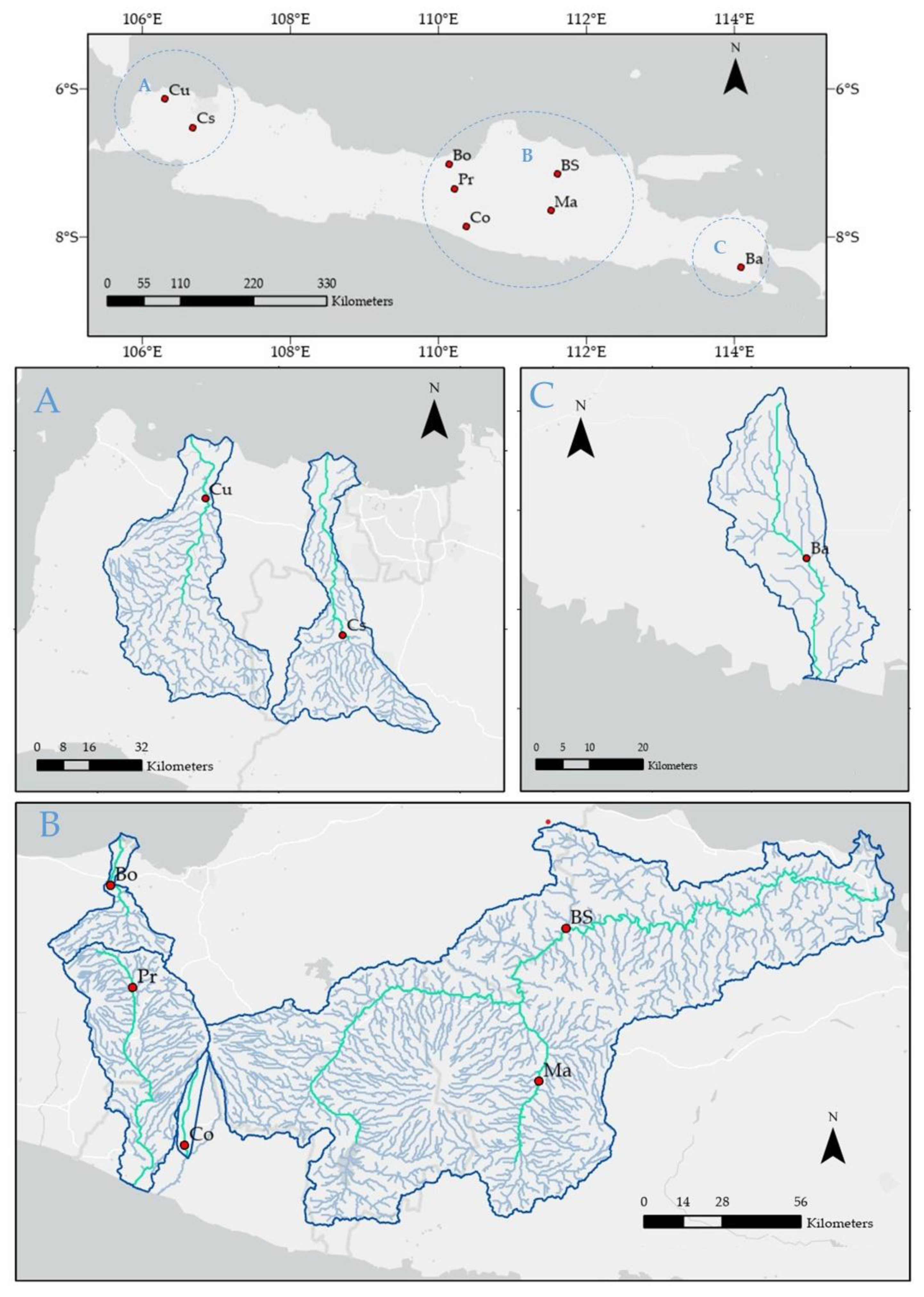
The streamflow data used in this study were obtained from the Research Center of Water Resource under the Ministry of Public Works Indonesia. The daily streamflow data from 1970–2018 of eight Indonesian rivers in Java Island were used. The eight rivers were Ciujung River (Cu), Cisadane River (Cs), Bodri River (Bo), Progo River (Pr), Bengawan Solo River (BS), Madiun River (Ma), Baru River (Ba), and Code River (Co). The profiles of those rivers can be found in

Table 1. Profiles of the streamflow gauge stations.

Code-Name	River Name	Flow Records Used (year)	Gauge’s Catchment Area (km2)	Region in Java	Gauge’s Location Coordinates
Cu	Ciujung	42	1562.7	West	−6.133, 106.300
Cs	Cisadane	44	850.2	West	−6.514, 106.678
Bo	Bodri	31	522.3	Central	−7.011, 110.137
Pr	Progo	38	423.4	Central	−7.340, 110.209
BS	Bengawan Solo	42	11,125.0	East	−7.150, 111.599
Ma	Madiun	30	2126.0	East	−7.645, 111.513
Ba	Baru	33	454.0	East	−8.413, 114.094
Co	Code	21	40.0	Central	−7.849, 110.375

, while their location can be seen in Figure 1.

The river selection is based on three criteria: temporal data quality, geographical location, and catchment area. Meanwhile, Co River is taken from our previous study for comparison. The data quality was first controlled by sorting the river gauges with minimum flow records of 30 years. Years with too many missing daily flows, as well as zero and interpolated flows, were omitted. To compare the effect of ENSO, which originated from the Pacific Ocean (east of Java), and IOD, which originated from the Indian Ocean (west of Java), we selected at least two rivers for each of eastern, western, and central regions of Java. Finally, we selected rivers that have catchment areas as similar as possible. However, due to the limitation from the other criteria, the selected rivers based on the catchment area became these three categories: <1000 km² (Cs, Bo, Pr, Ba), >1000 km² (Cu, Ma), and >10,000 km² (BS). For further information, the BS River is the largest river basin in Java which flows from Central Java to East Java.

The streamflow data analyzed in this study are in the form of flow regime indices based on the flow duration curve (FDC) definition. The FDC is a cumulative frequency curve that depicts the percentage of time that specified discharges were equaled or exceeded in a particular period [13]. This study used three flow regime indices, which are medium flow (Q₅₀), high flow (Q₁₀), and low flow (Q₉₀). With the definition of the FDC, Q₁₀ (Q₉₀) is the flow equaled or exceeded 10 (90) percent of all the time. Meanwhile, in data distribution, the definition of Q₁₀ (Q₉₀) is the 90th (10th) percentile due to the data ranking from lowest to highest. The three flow regimes were calculated using the R package fasstr [14].

2.2. Climate Indices

The ENSO indices used in this study were the Southern Oscillation Index (SOI) and the Niño 3.4, while Dipole Mode Index (DMI) was used for the IOD index. The DMI is the most commonly used index for IOD. SOI is the traditional ENSO index based on different sea level pressure between Darwin and Tahiti. It has been generally used in early [15] and recent [16] research. The Niño 3.4 is a sea surface temperature (SST) index, located in 5° N–5° S and 170° W–120° W, that has been acknowledged as the most representative index for ENSO [17], and was frequently used in many recent studies [18,19,20]. The SOI, Niño 3.4, and DMI data sets were obtained from the USA National Oceanic and Atmospheric Administration (NOAA).

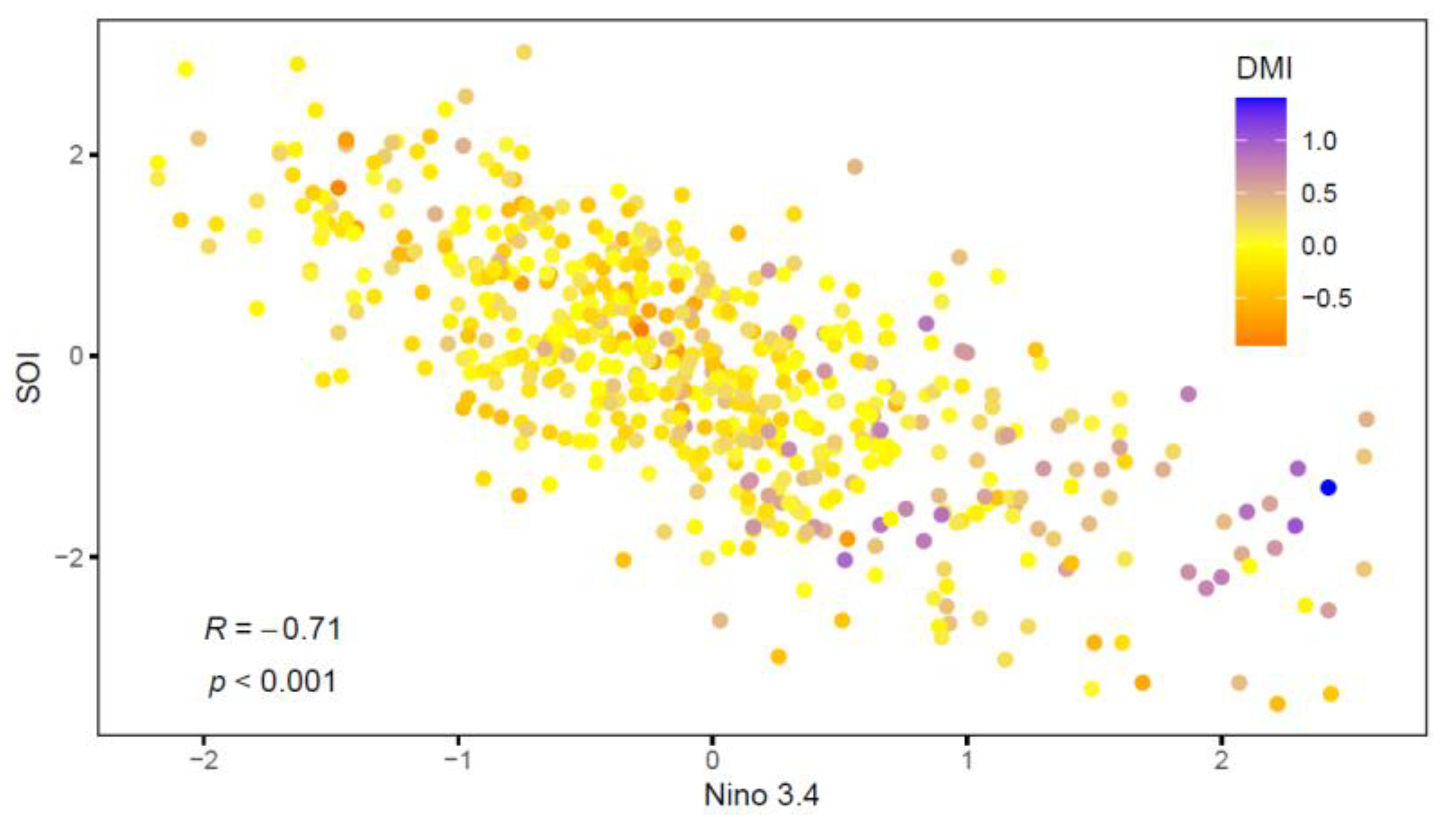
Our previous study [12] used SOI as the ENSO index while this study compared the monthly results of the two ENSO indices, SOI and Niño 3.4. The scatterplots in Figure 2 showed a correlation between the two ENSO indices using monthly data of 1970–2018. The correlation between the two indices was highly negative (R = −0.71), with high positive DMI mostly appearing in the El Niño phase (negative SOI, positive Niño 3.4). The SOI and Niño 3.4 did not differ by much in showing ENSO dynamics. Therefore, the results of our regression model from both climate indices were expected to be similar.

2.3. Temporal Variation Sets

This study attempted to find the best regression to explain ENSO and IOD variance in the streamflow data with four different sets. The first, second, and third sets are in monthly series, while the fourth sets are in the annual series. The first set is a series of monthly flows calculated from the distribution of daily flows. The second set is a six-month moving average series of monthly flow regime indices calculated from the average of the first series. The purpose of averaging over six months of monthly data is to reduce the effect of short timescale variation, such as Madden–Julian Oscillation (MJO) [21]. The third set is a series of seasonal monthly flows calculated as the first series in the three-monthly window of a season (explained below). The fourth set is a series of the seasonal average calculated by averaging the third set for each year.

Table 2. Temporal variation sets calculation method.

Set Name	Code-Name	Time Scale	Calculation Method
Ordinary monthly	MON	monthly flow	Q50: median of daily flow distribution in a month. Q90: 10% percentile of daily flow distribution in a month. Q10: 90% percentile of daily flow distribution in a month. Thus, there are 12 data sets for each year.
Six-month moving average	MA6	monthly flow with six-month information	Mean of each flow regime monthly series for six months. Thus, there are 12 data sets for each year.
Seasonal monthly (SM)	MAM/ JJA/ SON/ DJF	monthly flow	The same as with the ordinary monthly flow series, except the series is limited only to three months according to each season (e.g., Q50 of the MAM series includes the monthly Q50 of only March, April, and May, from 1970 to 2018). Thus, there are three data sets for each year.
Seasonal average (SMa)	MAMa/ JJAa/ SONa/ DJFa	three-month flow	Mean of the seasonal monthly series (e.g., the first datum in the MAMa series is the mean of three months: March, April, and May, in 1970). Thus, there is only one datum set for each year.

shows the detail of the streamflow data arrangement on each set. ENSO and IOD indices data sets followed the same temporal arrangement.

There are four seasons: March–April–May (MAM), June–July–August (JJA), September–October–November (SON), and December–January–February (DJF). The DJF series started from the year 1970, which consists of 1970 December, 1971 January, and 1971 February. This study strictly uses the period of 1970–2018, hence no 2019 data at all, even for DJF. Therefore, the period of the DJF series is 1970–2017, slightly different from the other three seasons, in which the period is 1970–2018.

2.4. Multiple Polynomial Regression

The regression analysis in this study used one of the ENSO indices (SOI or Niño 3.4) and DMI as predictors to predict Q₅₀ (medium flow), Q₁₀ (high flow), and Q₉₀ (low flow) for each river. Multiple regression (MR) models were developed using second-order and third-order polynomial functions to minimize the model’s error term as shown in Equations (1) and (2), respectively. All regression analyses and statistics in this study were carried out by using R programming [22,23].

y = β₀ + β₁x₁ + β₂x₂ + β₃x₁² + β₄x₂² + β₅x₁x₂ + ε

(1)

y = β₀ + β₁x₁ + β₂x₂ + β₃x₁² + β₄x₂² + β₅x₁x₂ + β₆x₁³ + β₇x₂³ + β₈x₁²x₂ + β₉x₁x₂² + ε

(2)

with:

y = flow regime index (Q₅₀/Q₁₀/Q₉₀)

x₁ = ENSO index (SOI/Niño 3.4)

x₂ = DMI

β = regression coefficient

ε = error term

2.5. Model Evaluation

The multiple polynomial regression in this study was evaluated by the adjusted coefficient of determination (adjusted R²) and the Kling–Gupta Efficiency (KGE) coefficient. The adjusted R² is commonly used to indicate the goodness of fit in models using multiple predictors. The KGE has been widely used in recent hydrological modeling studies. We used both evaluation metrics hoping that the result of our study can be easily compared to other studies, which use the common metric (R²) and the recently popular metric (KGE). The two evaluation metrics were calculated using the R package hydroGOF [24].

The adjusted R² is a better evaluation metric than the ordinary R² because it is adjusted by the number of observations and variables, resolving the bias issue in the ordinary R² caused by the degree of freedom problem. The adjusted R² is calculated by Equation (3) (n = number of observations, and p = number of predictors). The value of adjusted R² closer to 1 indicates better model skill.

$$R_{adjusted}^2=1-\left(1-R^2\right)\frac{n-1}{n-p-1}$$

(3)

The KGE coefficient is increasingly used in the recent hydrological modeling studies because it has been acknowledged to improve the famous model efficiency metric in hydrology, Nash–Sutcliffe Efficiency (NSE) [25,26]. The KGE coefficient is composed of three components: correlation (r), variability (standard deviation), and bias (mean). The values which can be considered to show any model skill are within −0.41 < KGE ≤ 1 [27], in which the model skill becomes better when the value is closer to 1. The metric of KGE will be more useful for future validation studies due to having a bias component. In this study, we used the modified KGE [28] by replacing the standard deviation (of the variability component) with the coefficient of variation (CV, ratio of standard deviation σ to mean μ) of each variable (Equation (4)).

$$KGE=1-\sqrt{{\left(r-1\right)}^2+{\left(\frac{C{V}_{sim}}{C{V}_{obs}}-1\right)}^2+{\left(\frac{{\mu }_{sim}}{{\mu }_{obs}}-1\right)}^2} , CV=\frac{\sigma }{\mu }$$

(4)

3. Results

3.1. Temporal Variability

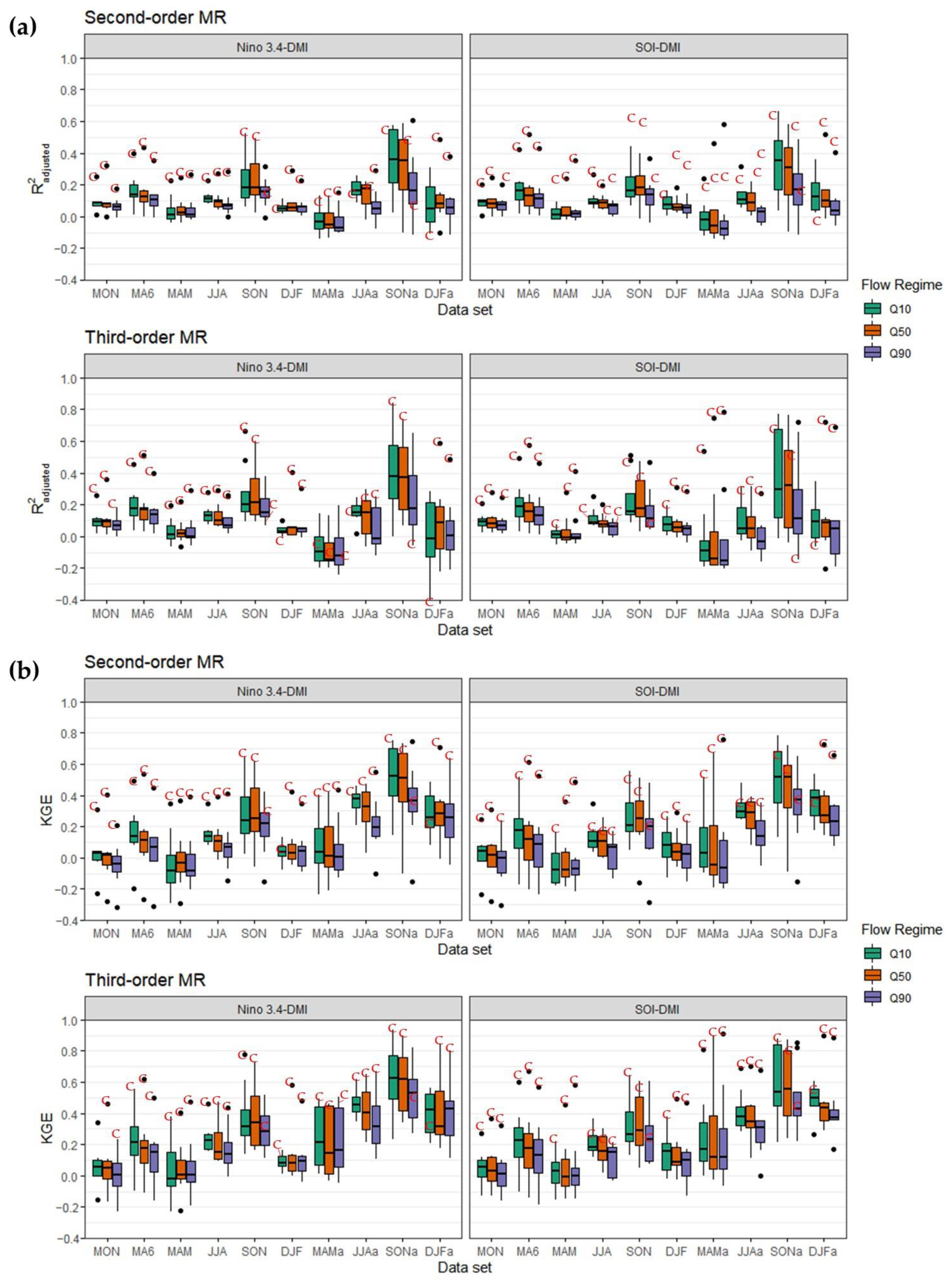
We applied the multiple regression (MR) analyses with the second- and third-order polynomial functions to find the best temporal variation set for regressing the indices of ENSO and IOD to the flow regime indices. The MR models were first developed by all possible variables. The model evaluation using adjusted R² and KGE coefficient (Figure 3) highlighted several points.

As shown in Figure 3, the regression of streamflow by ENSO and IOD indices is best achieved by the seasonal three-month average (SM_a) set in September–November (SON_a). The seasonal monthly (SM) from September–November (SON) also performed better among the SM sets. The results indicate two things. First, the streamflow predictability by ENSO and IOD was good only in the September–November season, when the transition from dry season to wet season usually occurs in the Java region [29]. Many previous studies have found a high correlation of ENSO and IOD during May–October or September–November to the rainfall [3,4,16,29,30,31] and streamflow [11] in the Java region. Second, in general, the SM_a sets have better model skills than the SM sets. This indicates that even with monthly data series in three-month windows, just ENSO and IOD are not enough to satisfy the need to describe the variance of the streamflows. The comparison between the monthly set (MON) and the six-month moving average set (MA6) also showed the same behavior. MA6 obtained a better model skill than MON due to MA6 carrying over the information of streamflow and climate indices for six months. Thus, it could filter the noises from other factors, such as another climate phenomenon with a shorter timescale, such as Madden–Julian Oscillation.

In general, the Q₅₀ and Q₁₀ models achieved better model skills than the Q₉₀. The overall distribution of Q₉₀ model skills is always lower than the other two regimes in SON and SON_a. It corresponds to the higher flow tending to be more sensitive in the regression with ENSO and IOD indices, as shown in our previous study for Code River [12]. Another previous study on a northwestern Java river showed that low stream flow events are related more to positive IOD based on a probability analysis [11]. However, our result cannot be compared directly to that study due to the different methods. While we used the ENSO and IOD indices together in multiple regression, that study treated them independently in simple probability and correlation analyses.

As expected, there were no significant differences between the model predicted by SOI-DMI and those by Niño 3.4-DMI. Only a few insignificant differences showed up in the maximum or minimum values of adjusted R² and KGE coefficients (Figure 3). It may also be worth noting that, in the averaged seasonal sets (MAM_a, JJA_a, SON_a, DJF_a) of the third-order models, the NINO 3.4 variant showed no KGE outliers. In contrast, the SOI variant has >10 KGE outliers. Meanwhile, there was no significant difference in KGE sets of the second-order models. This may indicate that in our case, the quality of the models developed in third-order MR is better when predicted by NINO 3.4 than SOI.

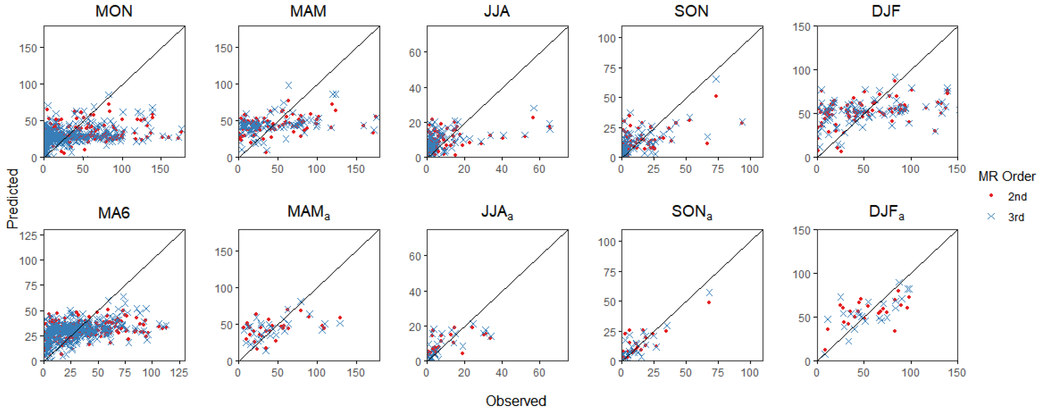
The results of the third-order MR were identified to be better than those of the second-order MR. The second (third)-order MR models for Q₁₀, Q₅₀, Q₉₀, which Niño 3.4-DMI predicted in the SON_a data set, have the maximum KGE of 0.75 (0.94), 0.74 (0.90), and 0.55 (0.82), respectively. Additionally, in the prediction by Niño 3.4-DMI in SON_a set, the outliers of the adjusted R² and KGE are found only in the second-order MR models. Overall, the third-order MR improved the model skills after the second-order MR, not only for the maximum but also for the minimum values of the evaluation metrics (Figure 3). The improvement of the predictability by the third-order models is more apparent in the higher flows, as shown by the example of Ma River in Figure 4.

It should be noted that a higher order polynomial function in a multiple regression model could reduce more degrees of freedom, causing model overfitting in the most extreme case. We discuss more details about this in Section 4.1 and Section 4.2.

3.2. Spatial Variability

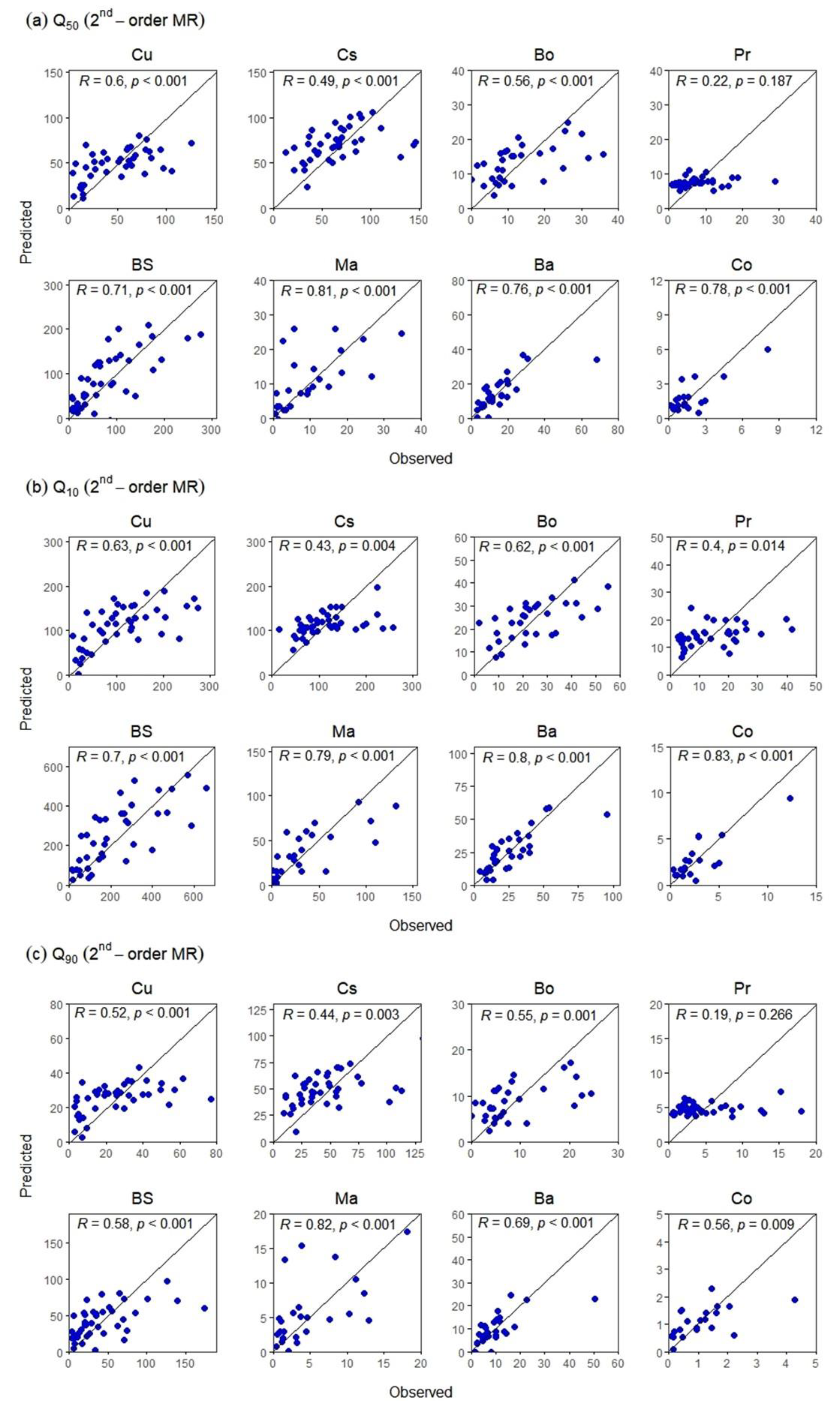
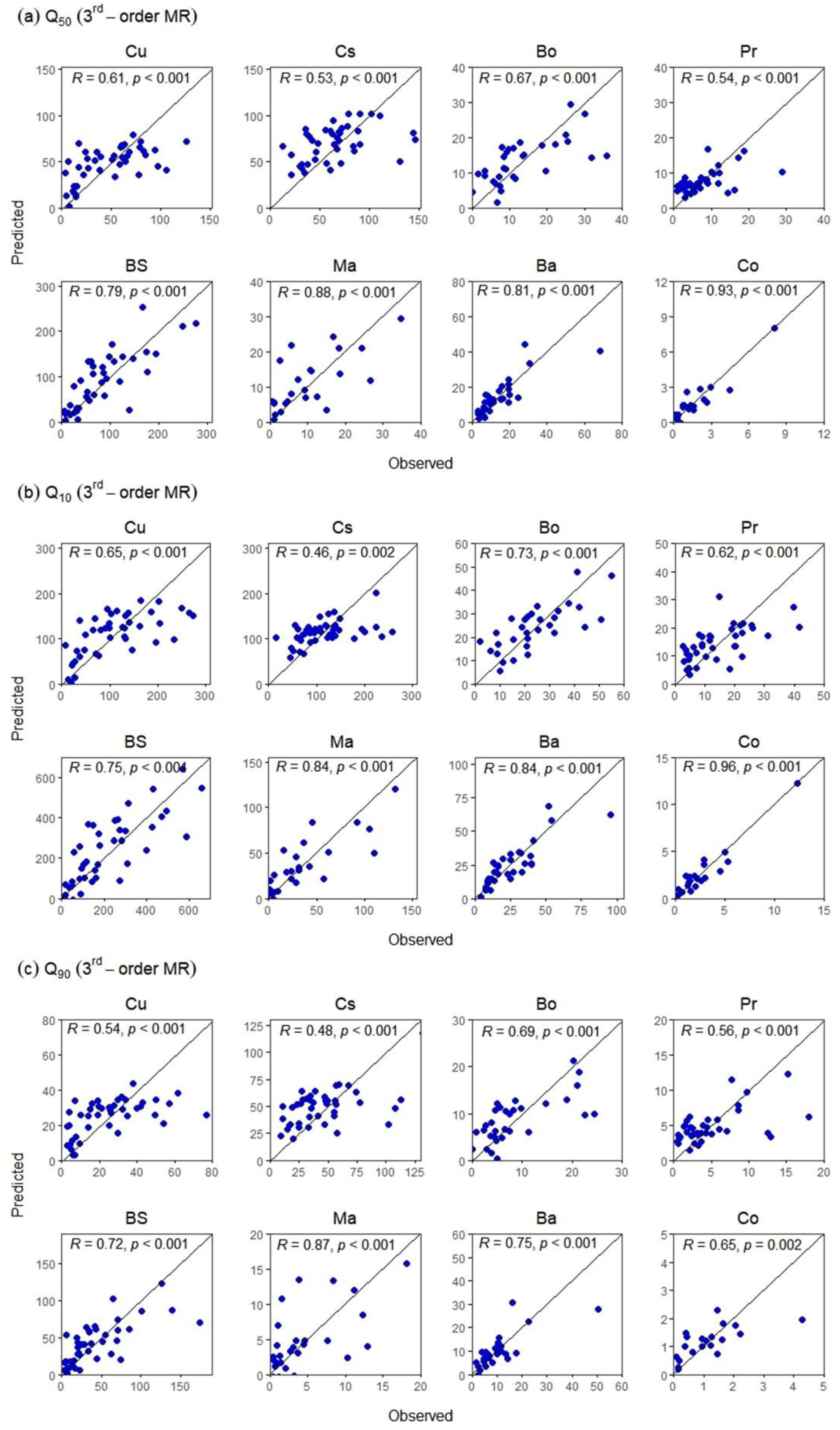
We knew from the previous section that the best model skill is found on the SON_a set. In Figure 2, the boxplots of the SON_a evaluation metrics are generally longer relative to the other sets, indicating a higher spatial variability among the temporal variation sets for all rivers. In this section, we attempted to explain the spatial variability among the rivers by analyzing the goodness of fit metrics (

Table 3. Adjusted R² for the models using Niño 3.4 and DMI as predictors in SON_a set. The values higher than 0.5 are bolded, indicating good model skill.

River	2nd-Order MR			3rd-Order MR
	Q50	Q10	Q90	Q50	Q10	Q90
Cu	0.28	0.17	0.31	0.19	0.10	0.26
Cs	0.14	0.09	0.08	0.09	0.03	0.00
Bo	0.18	0.16	0.26	0.21	0.26	0.33
Pr	−0.10	−0.12	0.02	0.07	0.09	0.19
BS	0.43	0.25	0.41	0.53	0.38	0.43
Ma	0.59	0.61	0.54	0.67	0.65	0.57
Ba	0.50	0.37	0.58	0.53	0.40	0.60
Co	0.48	0.08	0.57	0.74	−0.06	0.84

and

Table 4. KGE for the models using Niño 3.4–DMI as predictors in SON_a set. The values higher than 0.5 are bolded, indicating good model skill.

River	2nd-Order MR			3rd-Order MR
	Q50	Q10	Q90	Q50	Q10	Q90
Cu	0.24	−0.04	0.30	0.24	0.05	0.35
Cs	−0.15	−0.40	−0.44	0.00	−0.19	−0.31
Bo	0.11	0.06	0.28	0.41	0.46	0.54
Pr	−2.65	−3.48	−0.64	0.04	0.09	0.28
BS	0.49	0.17	0.47	0.67	0.52	0.58
Ma	0.70	0.72	0.65	0.82	0.80	0.75
Ba	0.61	0.44	0.68	0.70	0.59	0.76
Co	0.64	0.08	0.73	0.89	0.35	0.94

), the correlation between the predicted (by Niño 3.4-DMI in SON_a) and the observed flow regimes (

Table 5. Correlation coefficient (R Pearson) between the observed and the predicted flow regimes by Niño 3.4 and DMI in SON_a set. The values higher than 0.7 are bolded, indicating good model skill.

River	2nd-Order MR			3rd-Order MR
	Q50	Q10	Q90	Q50	Q10	Q90
Cu	0.60	0.63	0.52	0.61	0.65	0.54
Cs	0.49	0.43	0.44	0.53	0.46	0.48
Bo	0.56	0.62	0.55	0.67	0.73	0.69
Pr	0.22	0.40	0.19	0.54	0.62	0.56
BS	0.71	0.70	0.58	0.79	0.75	0.72
Ma	0.81	0.79	0.82	0.88	0.84	0.87
Ba	0.76	0.80	0.69	0.81	0.84	0.75
Co	0.78	0.83	0.56	0.93	0.96	0.65

). Generally, the west and the central rivers (Cu, Cs, Bo, Pr) have a lower predictability than the eastern rivers (BS, Ma, Ba). The western river models also tend to underestimate the higher flows, while the eastern river models’ estimations are spread evenly (Figure A1).

Ma River showed the best model skills (Table 3, Table 4 and Table 5) by consistently achieving excellent evaluation for all flow regimes and all MR orders. The scatterplots of second-order MR in Figure A1 showed that Ma River has some far-spread overestimation in the lower Q₅₀ and Q₉₀, even though their correlation coefficients (R) were higher than that of the Q₁₀. In that case, we can consider that another river in the same region, Ba, has more quality in prediction skill, due to having more consistently lower error distances. Only the highest flow of each flow regime in Ba River showed a relatively too far error distance, which underestimates by about 50% of the observed values. Those error distances were lowered in the third-order MR models (Figure A2).

Meanwhile, the Pr River in central Java consistently showed exceptionally poor model skills among all rivers in this study. With the negative values on KGE for all flow regimes, Pr becomes the only river that could not satisfy the minimum standard of KGE (−0.41) by the second-order MR modeling. The values of KGE (Table 3), adjusted R² (Table 4), and R of predicted–observed values (Table 5) all agree with the conclusion that Pr streamflow regimes cannot sufficiently develop a relationship model to the climate indices by MR analysis. Scatterplots of the second-order MR in Figure A1 showed more details that the predicted–observed correlation of Pr River is poor compared to those of the other rivers. Additionally, among the three flow regime indices of Pr River, only Q₁₀ could achieve a significant correlation to the observed values (Figure A1; the respective p-values for Q₅₀, Q₁₀, and Q₉₀ are 0.187, 0.014, and 0.266). In the third-order MR, the Pr River’s KGE (Table 4) and R (Table 5) values are become improved, passing the minimum standards (KGE > −0.41 and R > 0.50). However, the third-order MR models are still poor with the low KGE and adjusted R² values (Table 3). The scatterplots of predicted–observed values (Figure A2) also showed that the model skill of the third-order MR in the Pr River is more improved than that in the second-order MR (Figure A1). However, the spread of the plots does not make it a strong model.

In the end of this section, we can conclude that: (1) the eastern rivers could be predicted better than western and central rivers, (2) the Ma River in eastern Java achieved the highest model skill, and (3) the Pr River in central Java has the worst model skill. Although a minor point, it is also noted that the Bo River did not show a similar feature with the Pr River, although they are located in the same region. Instead, it showed a more similar quality to the western rivers, especially the Cu River. Many possible factors could affect the predictability difference among the rivers. We further investigated the tendency to conclude the reason for the different predictabilities in Section 4.

4. Discussion

4.1. Predictability Tendency by the Number of Observations

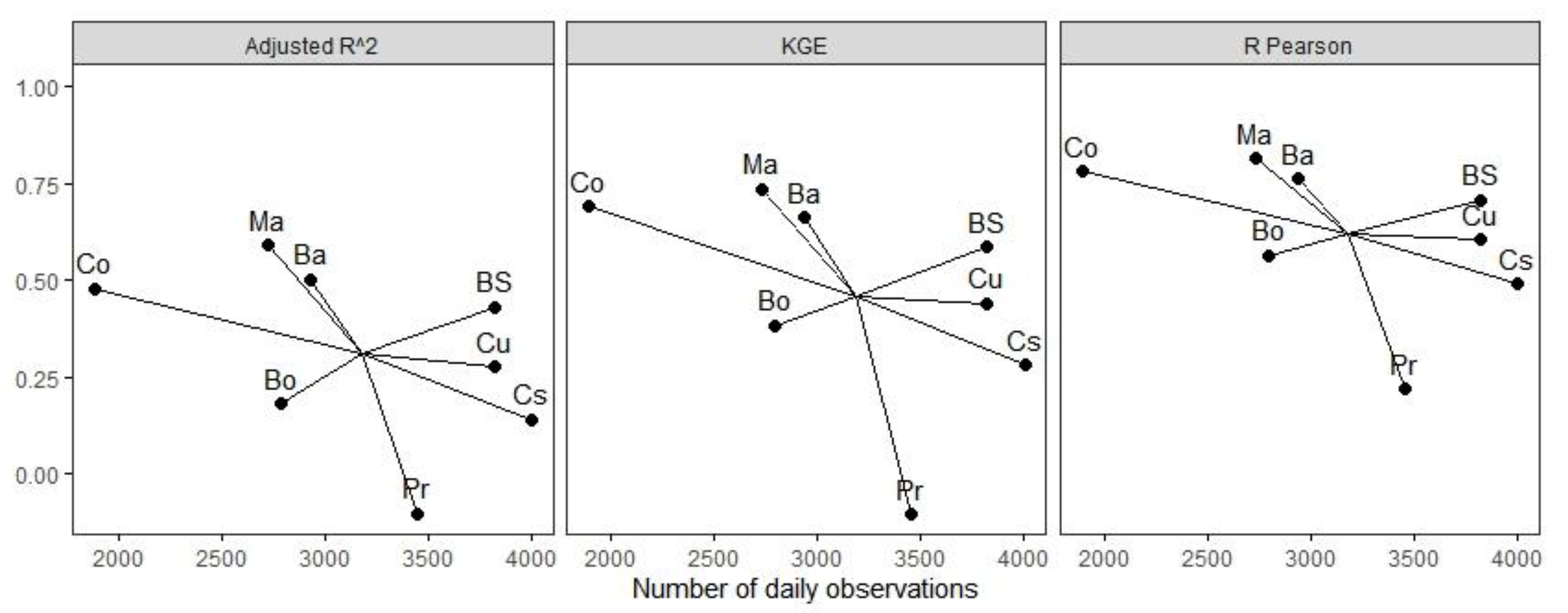
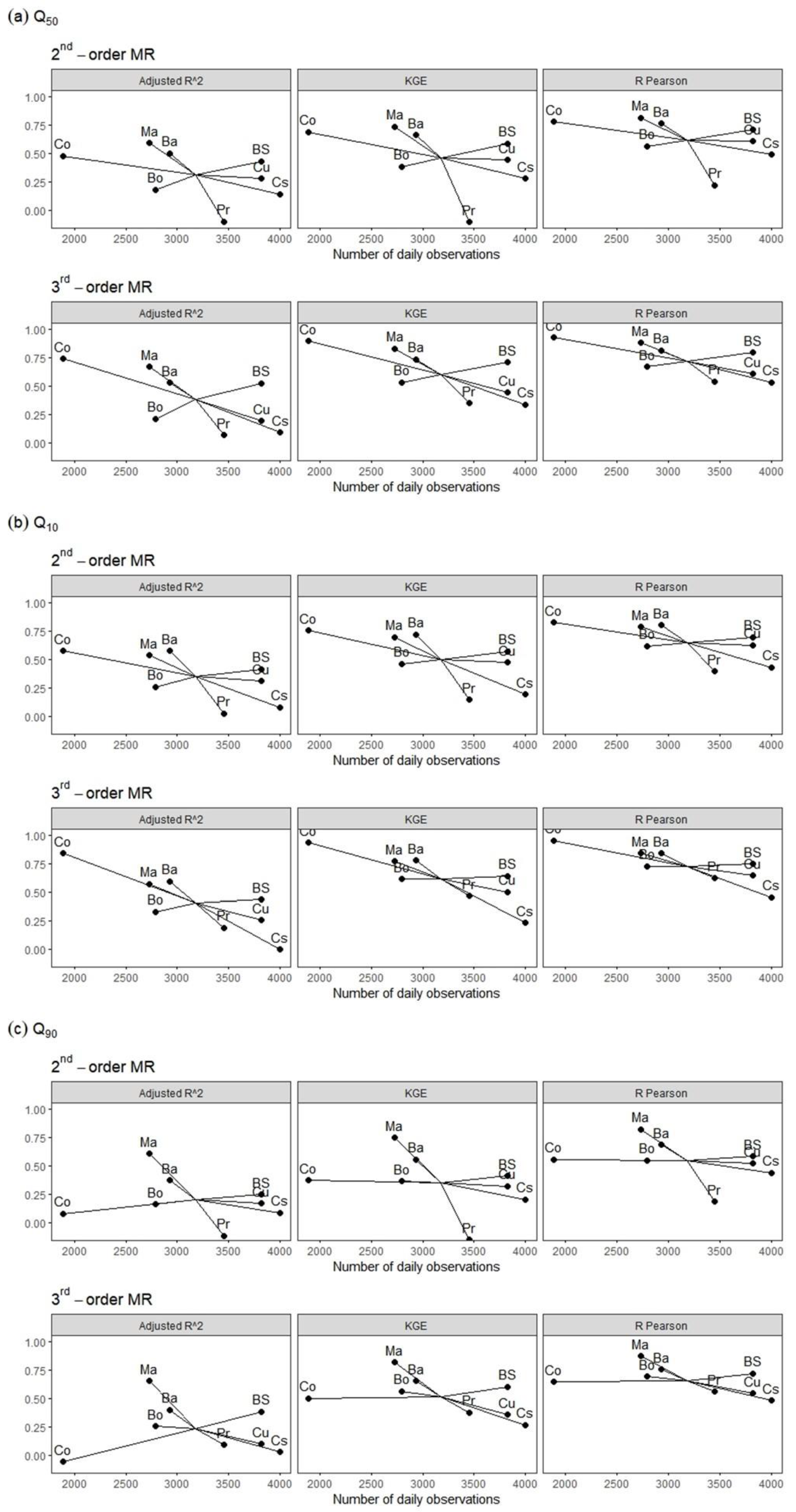
The rivers of Cu and Cs in western Java, along with the BS River in eastern Java, have the highest number of observations among the eight rivers in this study (Table 1). The model evaluation metrics (Table 3, Table 4 and Table 5) showed that the rivers of Cu and Cs have lower model skills than the eastern rivers. Typically, this phenomenon may be addressed on the problem of degree of freedom. A lower degree of freedom could lead to overfitting the regression model when dealing with higher order polynomial functions in a regression analysis. We looked further at the number of daily observations used on the models in SON_a and plotted them to the evaluation metrics (adjusted R², KGE, and R Pearson). Figure 5 shows the plots for Q₅₀ with the evaluation metrics for second-order MR models. Complete results for all flow regimes on second- and third-order MR models can be seen in Figure A3 in the Appendix B. All results showed similar tendency among the eight rivers. The BS River, which also has a large amount of data, similar to the rivers of Cu and Cs, could achieve a higher skill than the average, nearing the rivers of Ma and Ba (eastern rivers), which have the best skills among all. Meanwhile, Bo River, which has a similarly low number of observations as the Ma and Ba Rivers, had poor model skills. Pr River still had the lowest skills, despite it having more observations than Ma and Ba Rivers.

These results indicate that patterns related to the number of data and model skills may exist among the rivers, showing the difference in predictability under some spatial factors. The tendencies are probably not just that ‘‘higher amounts of data lead to lower model skill, and lower amounts of data lead to higher model skill’’. It is more likely indicating that the number of observations is not an issue related to the degree of freedom, affecting predictability. However, this argument is not quite strong enough to conclude this issue, so we continued the investigation by reanalyzing the data in the next subsection.

4.2. Change of Predictability over Periods

To resolve the degree of freedom issue, we reanalyzed the SON_a data sets from two different periods: 1970–1989 and 1990–2018. We recalculated new data sets which had been divided, then developed new regression models from them. This analysis may reduce the number of observations and become half of the original. Moreover, the number of parameters in the multiple polynomial regressions could further reduce the degree of freedom. Therefore, the second-order MR was used in this reanalysis due to having fewer parameters than third-order MR.

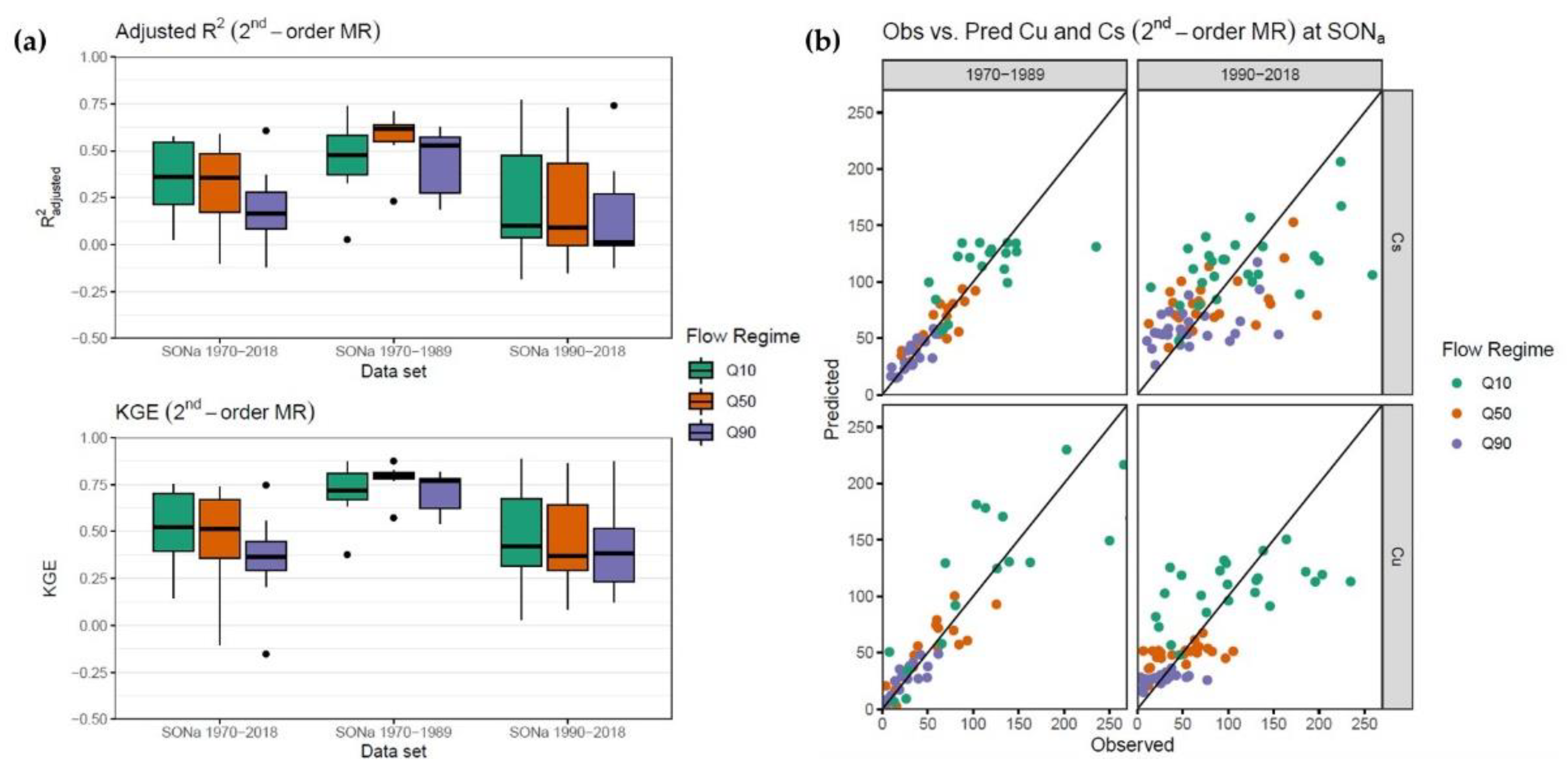
Figure 6 shows the result of the models’ evaluation for two periods. The results showed that the models in 1970–1989 (first period) generally have higher skills than those in 1990–2018 (second period). This is true for all flow regimes. Most rivers achieved good model skills in the first period, while in the second period, their model skills became poor mostly. On the other hand, the model skills of the original period (1970–2018) took place between the two periods. The complete adjusted R² and KGE values of the second- and third-order MR models in SON_a for the three periods are provided in

Table A1. Adjusted R² of the second-order MR models predicted by Niño 3.4 and DMI in SON_a set in three different periods. The values higher than 0.5 are bolded, indicating good model skill.

River	1970–2018			1970–1989			1990–2018
	Q50	Q10	Q90	Q50	Q10	Q90	Q50	Q10	Q90
Cu	0.277	0.309	0.170	0.618	0.478	0.568	0.090	0.100	−0.001
Cs	0.142	0.078	0.085	0.615	0.027	0.579	0.029	0.055	0.011
Bo	0.181	0.260	0.162	0.533	0.411	0.626	−0.037	0.022	−0.009
Pr	−0.101	0.025	−0.117	0.231	0.329	0.189	−0.149	−0.184	−0.122
BS	0.431	0.415	0.248	0.653	0.738	0.361	0.362	0.398	0.147
Ma	0.590	0.537	0.606	0.568	0.508	0.188	0.727	0.771	0.741
Ba	0.502	0.576	0.372	0.711	0.653	0.527	0.502	0.548	0.389
Co	-	-	-	-	-	-	0.479	0.575	0.078

,

Table A2. Adjusted R² of the third-order models predicted by Niño 3.4 and DMI in SON_a set in three different periods. The values higher than 0.5 are bolded, indicating good model skill.

River	1970–2018			1970–1989			1990–2018
	Q50	Q10	Q90	Q50	Q10	Q90	Q50	Q10	Q90
Cu	0.192	0.257	0.099	0.563	0.294	0.505	0.160	0.284	−0.048
Cs	0.093	−0.002	0.030	0.564	−0.326	0.560	−0.178	−0.148	−0.216
Bo	0.212	0.328	0.255	0.525	0.580	0.645	−0.222	−0.297	−0.060
Pr	0.065	0.188	0.091	0.540	0.648	0.318	−0.189	−0.253	0.040
BS	0.526	0.433	0.383	0.887	0.876	0.655	0.361	0.353	0.086
Ma	0.670	0.571	0.652	0.643	0.419	−0.254	0.863	0.893	0.839
Ba	0.530	0.596	0.401	0.625	0.514	0.300	0.708	0.674	0.653
Co	-	-	-	-	-	-	0.741	0.841	−0.058

,

Table A3. KGE of the second-order MR models predicted by Niño 3.4 and DMI in SON_a set in three different periods. The values higher than 0.5 are bolded, indicating good model skill.

River	1970–2018			1970–1989			1990–2018
	Q50	Q10	Q90	Q50	Q10	Q90	Q50	Q10	Q90
Cu	0.441	0.323	0.473	0.800	0.771	0.718	0.334	0.230	0.345
Cs	0.281	0.205	0.194	0.792	0.771	0.377	0.254	0.232	0.284
Bo	0.383	0.362	0.462	0.769	0.818	0.701	0.371	0.395	0.420
Pr	−0.105	−0.152	0.146	0.573	0.544	0.637	0.085	0.125	0.028
BS	0.587	0.410	0.572	0.826	0.657	0.870	0.575	0.383	0.604
Ma	0.735	0.747	0.696	0.797	0.586	0.767	0.865	0.872	0.887
Ba	0.663	0.555	0.719	0.875	0.789	0.849	0.711	0.634	0.741
Co	-	-	-	-	-	-	0.689	0.371	0.753

and

Table A4. KGE of the third-order MR models predicted by Niño 3.4 and DMI in SON_a set in three different periods. The values higher than 0.5 are bolded, indicating good model skill.

River	1970–2018			1970–1989			1990–2018
	Q50	Q10	Q90	Q50	Q10	Q90	Q50	Q10	Q90
Cu	0.441	0.356	0.502	0.858	0.837	0.761	0.560	0.417	0.637
Cs	0.337	0.268	0.230	0.847	0.845	0.453	0.287	0.251	0.314
Bo	0.533	0.564	0.615	0.875	0.907	0.890	0.597	0.659	0.567
Pr	0.351	0.375	0.464	0.863	0.792	0.897	0.387	0.536	0.339
BS	0.708	0.604	0.642	0.968	0.899	0.964	0.673	0.497	0.668
Ma	0.829	0.819	0.773	0.920	0.694	0.867	0.961	0.954	0.969
Ba	0.737	0.653	0.777	0.932	0.870	0.911	0.887	0.865	0.873
Co	-	-	-	-	-	-	0.895	0.500	0.937

in the Appendix C.

The scatterplots of predicted-observed rivers of Cu and Cs in Figure 6 clearly showed that the first period has better model skills. Cu and Cs are two examples of rivers in the lower model skills among the seven rivers in this study, placing them both in the lower parts of the boxplots, which shows the model skills among the rivers. The lower parts of the boxplots in Figure 6 showed that the first period achieved much better model skills than the second period, especially for the Q₅₀. Moreover, the model skill of the original period with all the data from both periods naturally became lower than the first period and higher than the second period. These results indicate that the rivers of Cu and Cs did not always have a poor relationship with the ENSO and IOD. Instead, it suggests that the relationship in the first period was changed in the second period.

The relationship changes in the western Java rivers were probably caused by the human perturbation to the river basin, such as land-use change and the development of the river. The start of the river development era in Indonesia might be related to this phenomenon. River development means that rivers were physically changed—such as meander cutoff, riverbank narrowing, adding irrigation weir, and dam building—thus, it becomes more unnatural and changes the hydrological processes of streamflow. In Indonesia, these structural modifications to rivers started to grow rapidly around 1990, especially in the region of Java [32]. The construction of several dams could be identified around that time, such as Pongkor Dam in Cs River (1996) [33] and Wonogiri Dam in BS River (1981) [34]. At that time, the purpose of the structural changes was mostly for agriculture use. Such physical changes may alter the hydrological processes in the watershed, thus giving a different relationship between climate and streamflow. Therefore, one reason that the relationship between ENSO and IOD to the streamflow could be better predicted before 1990 might be due to the rivers still being more natural than those in the next period (1990–2018).

4.3. Good Predictability in Code River

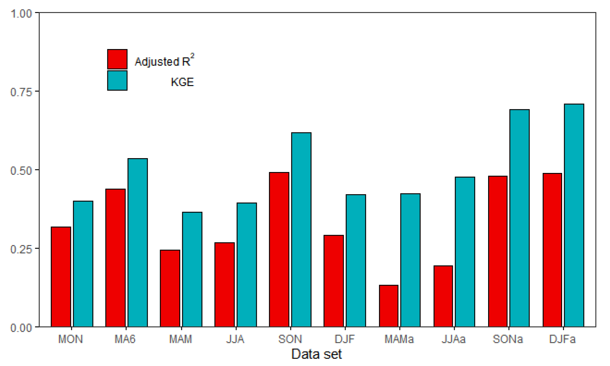
In our previous study [12], we obtained good predictability of the Code (Co) River streamflow by SOI-DMI predictors. In this paper, the Code River data were reanalyzed further with the seasonal and the averaged seasonal sets, achieving higher model skills than the six-month moving average data set (MA6). The result of spatiotemporal analysis in this study indicates that Code River has lower seasonal variability than the other rivers. Code River’s model skills are consistently at the maximum point in all rivers’ evaluation metrics distribution (Figure 3), sometimes shown as outliers.

The MA6 data set represents intra-annual variation, while SON and SON_a are not. It can be understood that if a river showed high MA6 model skill, its relationship to the climate indices in intra-annual variation is also high. Meanwhile, we knew that, among the four seasons, only the SON season gives the best model skill. Hence, if MA6′s model skill is high, then it must be due to low intra-annual (seasonal) variation, in which the predictability of the other three seasons is not too different from the SON season.

We already knew that the predictability of Code River is good in SON sets, just like the other rivers. Meanwhile, the MA6 set of Code River also showed relatively good predictability. However, the other rivers could not achieve the same quality of MA6 as Code River (Figure 3). Therefore, it can be concluded that Code River has a lower intra-annual variation than the other rivers. Figure 7 showed that the predictability of Q₅₀ of Code River is similar in SON_a and DJF_a, while MAM_a and JJA_a were about 0.25 lower. Hence, the intra-annual predictability of Code River is relatively low. Therefore, we concluded that the excellent model skill obtained by Code River in our previous paper seems to be owing to its seasonal characteristic.

Additionally, when comparing the catchment area of Code River to those of the other seven rivers, it could be seen that the small catchment area of Code River is an outlier. Hence, it can be assumed that the small catchment area of Code River may contribute to the good predictability of Code River. However, before this study, we have tried to connect the ENSO and IOD indices to a few other small catchment rivers near the Code River (such as Tambakbayan and Gajahwong Rivers) but could not get results as good as that in the Code River case. Hence, a smaller catchment area may, but not necessarily, improve the relationship between climate and streamflow.

4.4. Streamflow Prediction by ENSO and IOD

Our study results showed that the ENSO and IOD teleconnection to flow regimes in Java rivers only appeared good in the SON season (the onset of wet season [29]), with averaged set (SON_a) better than the monthly set (SON). It emphasizes that intra-annual variation is crucial to be considered in studying the relationship between climate indices and the streamflow or rainfall in Indonesia. Despite Indonesia having only two seasons (wet and dry), intra-annual variation is still important to be considered, owing to many interrelated climate phenomena around the regions in different periods and timescales.

Considering the results of spatial variability analysis, we suggest that the teleconnections for climate–rainfall and climate–streamflow are not necessarily similar. The physical processes in the climate–streamflow teleconnection are more complex than those in the climate–rainfall teleconnection. In the climate–streamflow relationship, physical processes are mainly related to the hydrological processes, such as runoff generation and evaporation. It has been known that anthropogenic activities could directly affect the hydrological processes [35,36]. Therefore, different physical conditions of a watershed due to human perturbation could create a large variation in the climate–streamflow relationship, even though the rivers are located in the same region. In this case, not only spatial variability but temporal variability could also be related to the hydrological changes of a river basin, as discussed in Section 4.2.

Good predictability of flow regimes by ENSO and IOD would be useful in forecasting the streamflow. In this study, we did not forecast the streamflow by the two climate indices. Instead, we successfully elucidated the connection between the indices of two climate phenomena and streamflow indices in simultaneous seasons diagnostically. As good progress was shown in the prediction of ENSO [37] and IOD [38], now we can forecast them more accurately. If we can accurately forecast ENSO and IOD, we can also accurately forecast the streamflow regimes using a skilled teleconnection model. The forecast of extreme flow events could lead to better mitigation of water-related disasters. For that reason, the knowledge of climate teleconnections to the streamflow is very useful for river managers.

However, there is a difference in predictability skills between high flow and low flow found in our study. Based on our study results, high flow index (Q₁₀) and medium flow index (Q₅₀) could be predicted better than low flow index (Q₉₀). While the Q₁₀ predictability level seemed similar among rivers in Java, Q₉₀ was the opposite. The different predictability of Q₉₀ from one river to another is probably caused by the low flow dependency on the physical condition of a river’s watershed. Anthropogenic drought problems, such as land-use change and groundwater exploitation, make Q₉₀ prediction by climate harder. Meanwhile, high flow situations, even in flood, are usually linear to the amount of rainfall (hence climate), making the prediction of Q₁₀ by climate better than Q₉₀.

5. Conclusions

This study developed the relationship between river flow regimes in Java and climate indices of ENSO and IOD by multiple regression (MR) models in ten different temporal data sets. We obtained good predictability of the flow regimes using the ENSO and IOD indices in September–November (SON), especially with the averaged SON set (SON_a). The high predictability in the SON season is consistent with the previous studies on ENSO and IOD indices’ connections to rainfall [16,31] and streamflow [11] in Indonesia. Here, we advanced the simple correlation analysis in past studies to multiple polynomial regression and achieved new insights into the prediction of Indonesian streamflow by both ENSO and IOD indices.

Spatial variability analysis showed no clear distribution pattern of predictability over the Javanese rivers. The difference in model skills among the eight rivers in Java does not seem to be due to the regional distribution effects of ENSO and IOD; instead, the characteristics of each river are suggested to be the main cause. We compared the teleconnection of two different periods, 1970–1989 and 1990–2018. Interestingly, the first period bestowed better prediction skills, most likely due to physical changes caused by river development, thereby weakening the climate–streamflow relationship over the years.

The difference between climate–rainfall and climate–streamflow relationships could be seen from their spatial variabilities caused by the different hydrological processes in river basins. The hydrological processes in each river basin often varied significantly, caused mainly by anthropogenic disturbance. This disturbance could also be detected in the temporal variations by comparing the predictability in different periods. As for our case, different predictabilities were found between the periods of 1970–1989 and 1990–2018. Therefore, we could assume that the difference was due to the relationship change before and after the disturbance.

The Code River, featured in our previous work [12], was included in this study to compare and better understand the teleconnection with rivers in the same region. We achieved good model skills of the Code River in the previous study, with a six-month moving average set, and the current study, with seasonal data sets. However, the other seven rivers in this study showed varied quality in model skills, caused by the lower intra-annual variation and higher inter-annual variation that the Code River had compared with the other rivers. Therefore, our previous work results could be a fortunate case for finding a good flow regime predictability for a river.

This study contributes to the new understanding of ENSO and IOD relationship to the streamflow in Indonesia. Our result showed new insights into the relationship using flow regimes and spatiotemporal analysis. Varied predictability skills were found among the three flow regimes and the eight rivers in Java. The predictability of the high flow regime tends to be higher than that of the low flow regime over many rivers in Java. From the eight rivers, we found that the rivers of Ma, Ba, and Co could be better predicted than the rest of the rivers.

Future works can be aimed toward forecasting the streamflow regimes, as it will be useful for river managers. A further investigation aimed at forecasting could be done by studying the lead-lag relationship between the climate indices and the streamflow regimes. Another future study should be on improving the teleconnection model. To improve the predictability skill of the flow regimes, it might be a good idea to incorporate components from the physical processes in the watershed or apply more advanced data filtering and modeling methods.

References

- Poff, N.L. Beyond the natural flow regime? Broadening the hydro-ecological foundation to meet environmental flows challenges in a non-stationary world. Freshw. Biol. 2018, 63, 1011–1021. [Google Scholar] [CrossRef]
- Ropelewski, C.F.; Halpert, M.S. Global and Regional Scale Precipitation Patterns Associated with the El Niño/Southern Oscillation. Mon. Weather Rev. 1987, 115, 1606–1626. [Google Scholar] [CrossRef] [Green Version]
- Hendon, H.H. Indonesian rainfall variability: Impacts of ENSO and local air-sea interaction. J. Clim. 2003, 16, 1775–1790. [Google Scholar] [CrossRef]
- Aldrian, E.; Susanto, R.D. Identification of three dominant rainfall regions within Indonesia and their relationship to sea surface temperature. Int. J. Climatol. 2003, 23, 1435–1452. [Google Scholar] [CrossRef]
- Lee, H.S. General Rainfall Patterns in Indonesia and the Potential Impacts of Local Seas on Rainfall Intensity. Water 2015, 7, 1751–1768. [Google Scholar] [CrossRef]
- Saji, N.; Goswami, B.; Vinayachandran, P.; Yamagata, T. A dipole mode in the Tropical Ocean. Nature 1999, 401, 360–363. [Google Scholar] [CrossRef]
- Cardoso, A.O.; Silva Dias, P.L. The relationship between ENSO and Paraná River flow. Adv. Geosci. 2006, 6, 189–193. [Google Scholar] [CrossRef] [Green Version]
- Cluis, D.; Laberge, C. Analysis of the El Niño Effect on the Discharge of Selected Rivers in the Asia-Pacific Region. Water Int. 2002, 27, 279–293. [Google Scholar] [CrossRef]
- Zhang, Q.; Xu, C.Y.; Jiang, T.; Wu, Y. Possible influence of ENSO on annual maximum streamflow of the Yangtze River, China. J. Hydrol. 2007, 333, 265–274. [Google Scholar] [CrossRef]
- Mohsenipour, M.; Shahid, S.; Nazemosadat, M.J. Effects of El Nino Southern Oscillation on the Discharge of Kor River in Iran. Adv. Meteorol. 2013, 2013, 1–7. [Google Scholar] [CrossRef]
- Sahu, N.; Behera, S.K.; Yamashiki, Y.; Takara, K.; Yamagata, T. IOD and ENSO impacts on the extreme stream-flows of Citarum River in Indonesia. Clim. Dyn. 2012, 39, 1673–1680. [Google Scholar] [CrossRef]
- Nugroho, A.R.; Tamagawa, I.; Harada, M. The Relationship between River Flow Regimes and Climate Indices of ENSO and IOD on Code River, Southern Indonesia. Water 2021, 13, 1375. [Google Scholar] [CrossRef]
- Searcy, J.K. Flow-Duration Curves; United States Government Printing Office: Washington, DC, USA, 1959. [Google Scholar] [CrossRef]
- Goetz, J.; Schwarz, C.J. Fasstr: Analyze, Summarize, and Visualize Daily Streamflow Data, R package version 0.3.3; CRAN, 2021; Available online: https://cran.r-project.org/package=fasstr (accessed on 29 November 2021).
- Ropelewski, C.F.; Halpert, M.S. Precipitation Patterns Associated with the High Index Phase of the Southern Oscillation. J. Clim. 1989, 2, 268–284. [Google Scholar] [CrossRef] [Green Version]
- Kurniadi, A.; Weller, E.; Min, S.K.; Seong, M.G. Independent ENSO and IOD impacts on rainfall extremes over Indonesia. Int. J. Climatol. 2021, 41, 3640–3656. [Google Scholar] [CrossRef]
- Bamston, A.G.; Chelliah, M.; Goldenberg, S.B. Documentation of a Highly ENSO-Related SST Region in the Equatorial Pacific: Research Note. Atmos.-Ocean 1997, 35, 367–383. [Google Scholar] [CrossRef]
- Hendrawan, I.G.; Asai, K.; Triwahyuni, A.; Lestari, D.V. The interanual rainfall variability in Indonesia corresponding to El Niño Southern Oscillation and Indian Ocean Dipole. Acta Oceanol. Sin. 2019, 38, 57–66. [Google Scholar] [CrossRef]
- Rao, J.; Ren, R. Parallel comparison of the 1982/83, 1997/98 and 2015/16 super El Niños and their effects on the extratropical stratosphere. Adv. Atmos. Sci. 2017, 34, 1121–1133. [Google Scholar] [CrossRef]
- Qian, H.; Xu, S.-B. Prediction of Autumn Precipitation over the Middle and Lower Reaches of the Yangtze River Basin Based on Climate Indices. Climate 2020, 8, 53. [Google Scholar] [CrossRef] [Green Version]
- Hidayat, R.; Kizu, S. Influence of the Madden-Julian Oscillation on Indonesian rainfall variability in austral summer. Int. J. Climatol. 2010, 30, 1816–1825. [Google Scholar] [CrossRef]
- R Core Team. R: A Language and Environment for Statistical Computing, R version 4.1.2; 2021; Available online: http://www.r-project.org/ (accessed on 29 November 2021).
- Wickham, H. Modelr: Modelling Functions that Work with the Pipe, R package version 0.1.8; CRAN, 2020; Available online: https://cran.r-project.org/package=modelr (accessed on 29 November 2021).
- Zambrano-Bigiarini, M. Hydrogof: Goodness-of-Fit Functions for Comparison of Simulated and Observed Hydrological Time Series, R package version 0.4-0; CRAN, 2020; Available online: https://cran.r-project.org/package=hydroGOF (accessed on 29 November 2021).
- Nash, J.E.; Sutcliffe, J.V. River flow forecasting through conceptual models part I—A discussion of principles. J. Hydrol. 1970, 10, 282–290. [Google Scholar] [CrossRef]
- Gupta, H.V.; Kling, H.; Yilmaz, K.K.; Martinez, G.F. Decomposition of the mean squared error and NSE performance criteria: Implications for improving hydrological modelling. J. Hydrol. 2009, 377, 80–91. [Google Scholar] [CrossRef] [Green Version]
- Knoben, W.J.M.; Freer, J.E.; Woods, R.A. Technical note: Inherent benchmark or not? Comparing Nash-Sutcliffe and Kling-Gupta efficiency scores. Hydrol. Earth Syst. Sci. 2019, 23, 4323–4331. [Google Scholar] [CrossRef] [Green Version]
- Kling, H.; Fuchs, M.; Paulin, M. Runoff conditions in the upper Danube basin under an ensemble of climate change scenarios. J. Hydrol. 2012, 424–425, 264–277. [Google Scholar] [CrossRef]
- Hamada, J.I.; Yamanaka, M.D.; Matsumoto, J.; Fukao, S.; Winarso, P.A.; Sribimawati, T. Spatial and temporal variations of the rainy season over Indonesia and their link to ENSO. J. Meteorol. Soc. Japan 2002, 80, 285–310. [Google Scholar] [CrossRef] [Green Version]
- Jun-Ichi, H.; Mori, S.; Kubota, H.; Yamanaka, M.D.; Haryoko, U.; Lestari, S.; Sulistyowati, R.; Syamsudin, F. Interannual rainfall variability over northwestern Jawa and its relation to the Indian Ocean Dipole and El Niño-Southern Oscillation events. Sci. Online Lett. Atmos. 2012, 8, 69–72. [Google Scholar] [CrossRef] [Green Version]
- Hidayat, R.; Ando, K.; Masumoto, Y.; Luo, J.J. Interannual Variability of Rainfall over Indonesia: Impacts of ENSO and IOD and Their Predictability. IOP Conf. Ser. Earth Environ. Sci. 2016, 31, 012043. [Google Scholar] [CrossRef]
- Maryono, A. River Restoration, 4th ed.; Gadjah Mada University Press: Yogyakarta, Indonesia, 2020; ISBN 978-979-420-667-6. [Google Scholar]
- Kali Cisadane. Catalogue of Rivers for Southeast Asia and the Pacific-Volume V; Tachikawa, Y., James, R., Abdullah, K., Desa, M.N.b.M., Eds.; The UNESCO-IHP Regional Steering Committee for Southeast Asia and the Pacific, 2004; pp. 45–56. ISBN 4-902712-00-8. Available online: https://hywr.kuciv.kyoto-u.ac.jp/ihp/riverCatalogue/Vol_05/index.html (accessed on 29 November 2021).
- Bengawan Solo. In Catalogue of Rivers for Southeast Asia and the Pacific-Volume I; Takeuchi, K.; Jayawardena, A.W.; Takahasi, Y. (Eds.) The UNESCO-IHP Regional Steering Committee for Southeast Asia and the Pacific, 1995; pp. 91–102. ISBN 962-8014-07-2. Available online: https://hywr.kuciv.kyoto-u.ac.jp/ihp/riverCatalogue/Vol_01/index.html (accessed on 29 November 2021).
- Gornitz, V.; Rosenzweig, C.; Hillel, D. Effects of anthropogenic intervention in the land hydrologic cycle on global sea level rise. Glob. Planet. Change 1997, 14, 147–161. [Google Scholar] [CrossRef]
- Vorosmarty, C.J.; Sahagian, D. Anthropogenic disturbance of the terrestrial water cycle. Bioscience 2000, 50, 753–765. [Google Scholar] [CrossRef] [Green Version]
- Tang, Y.; Zhang, R.H.; Liu, T.; Duan, W.; Yang, D.; Zheng, F.; Ren, H.; Lian, T.; Gao, C.; Chen, D.; et al. Progress in ENSO prediction and predictability study. Natl. Sci. Rev. 2018, 5, 826–839. [Google Scholar] [CrossRef]
- Feba, F.; Ashok, K.; Collins, M.; Shetye, S.R. Emerging Skill in Multi-Year Prediction of the Indian Ocean Dipole. Front. Clim. 2021, 3, 1–8. [Google Scholar] [CrossRef]
Figure 1.
Location of the selected rivers in Java Island, Indonesia.
Figure 2.
Scatterplot of SOI and Niño 3.4 with DMI levels (1970–2018).
Figure 3.
Boxplot series showing model’s evaluation metrics of (a) adjusted R2 and (b) KGE coefficient with two variants of predictor combinations: NINO 3.4-DMI and SOI-DMI. The x-axis shows the temporal variation sets (MON: monthly flow, MA6: six-month moving average flow, MAM-DJF: monthly flow in the window of each respective season, MAMa-DJFa: three-month average flow in the window of each respective season). C = Code River. The lines in the middle of the box are median. The top of the box is the third quartile (Q3), and the bottom is the first quartile (Q1). The vertical lines above and below the box show the data range, excluding outliers. The dots represent outliers, values that are farther than 1.5 times of their interquartile ranges (IQR = Q3 − Q1).
Figure 4.
Scatterplots between the predicted (using second- and third-order MR models with Niño 3.4 and DMI as predictors) and the observed Q50 for Madiun River (Ma) in all temporal variants: monthly (MON), six-month moving average (MA6), monthly seasonal (MAM-DJF), and averaged monthly seasonal (MAMa-DJFa).
Figure 5.
Plot between the number of daily observations (x-axis) for Q50 models (second-order) in the SONa set and their model skills (y-axis).
Figure 6.
(a) Evaluation metrics boxplots and (b) predicted–observed scatterplots of MR models (2nd-order, Niño 3.4–DMI predictors, SONa set) with three different window periods: 1970–2018, 1970–1989, and 1990–2018. The boxplots show the metrics for all rivers, while the scatterplots only show the plots for Cs and Cu Rivers.
Figure 7.
The adjusted R2 and KGE of Code River’s Q50 second-order MR models in different temporal data sets.