Swin Transformer for Complex Coastal Wetland Classification Using the Integration of Sentinel-1 and Sentinel-2 Imagery

Abstract

The emergence of deep learning techniques has revolutionized the use of machine learning algorithms to classify complicated environments, notably in remote sensing. Convolutional Neural Networks (CNNs) have shown considerable promise in classifying challenging high-dimensional remote sensing data, particularly in the classification of wetlands. State-of-the-art Natural Language Processing (NLP) algorithms, on the other hand, are transformers. Despite the fact that transformers have been utilized for a few remote sensing applications, they have not been compared to other well-known CNN networks in complex wetland classification. As such, for the classification of complex coastal wetlands in the study area of Saint John city, located in New Brunswick, Canada, we modified and employed the Swin Transformer algorithm. Moreover, the developed transformer classifier results were compared with two well-known deep CNNs of AlexNet and VGG-16. In terms of average accuracy, the proposed Swin Transformer algorithm outperformed the AlexNet and VGG-16 techniques by 14.3% and 44.28%, respectively. The proposed Swin Transformer classifier obtained F-1 scores of 0.65, 0.71, 0.73, 0.78, 0.82, 0.84, and 0.84 for the recognition of coastal marsh, shrub, bog, fen, aquatic bed, forested wetland, and freshwater marsh, respectively. The results achieved in this study suggest the high capability of transformers over very deep CNN networks for the classification of complex landscapes in remote sensing.

1. Introduction

Wetlands are territories that have been immersed in water for long enough to generate hydric soils and support the growth of hydrophytic or water-tolerant plants [1,2,3]. Wetlands can be found practically everywhere on the planet, from the tundra to the tropics, and are an important aspect of the natural habitat [1,4,5,6,7]. Although the importance of wetlands for fish and animal conservation has been recognized for over a century, some of the other benefits have only lately been discovered. Because they operate as downstream recipients of water and waste from both natural and human sources, wetlands are sometimes referred to as the natural environment’s kidneys [4]. They help to stabilize the water supply, reducing the risk of flooding and drought [8,9]. It has been discovered that they can clean polluted rivers, safeguard shorelines, and recharge groundwater aquifers. Because of the wide food chain and diverse biodiversity that they support, wetlands have been dubbed “nature’s supermarkets.” In ecosystem service assessments, wetlands are still considered the most valuable aspects of our environment [4,10,11]. Wetland species, on the other hand, account for 24% of the world’s invasive plants, despite accounting for only 6% of global land cover [12]. Invasive species pose a serious risk to coastal wetlands since they can form dense, monolithic stands, out-competing native species and affecting wetlands’ structure [12]. A coastal wetland is defined as an area between the lower subtidal zone, where sunlight can penetrate and sustain photosynthesis by benthic plant communities, and the landward border, where the sea’s hydrologic impact is relinquished to groundwater and atmospheric processes [13]. Considering the multiple stressors that wetlands face from human activities, invasive species, and climate change, proper management and monitoring methods are required to ensure wetland conservation and protection. Wetland mapping with high spatial and thematic precision is crucial for wetland management and monitoring. These maps aid in identifying wetlands’ vulnerabilities and pressures and assessing the efficacy of wetland conservation strategies.

Wetland conservation programs exist in New Brunswick and numerous other Canadian provinces, but their successful implementation requires an accurate and up-to-date wetland map. The cost-effectiveness and quality of data sources, subsequent studies, and ground-truthing are all important factors in producing reliable wetland maps [14]. Wetland mapping on a large scale has traditionally been problematic given the cost of data collection and wetland ecosystems’ highly dynamic and remote nature. Long-term wetland observation in Canada demands a significant amount of fieldwork and long-term human commitment and financing. As a result, remote sensing data acquisition brings up hitherto unimagined opportunities for large-scale wetland analysis [15,16,17,18,19]. While remote sensing, like every instrument, has limitations when it comes to wetland mapping and monitoring, it offers some advantages that make it a good fit for these tasks. Remote sensing, for instance, saves money and time by eliminating the requirement for site visits while still covering vast geographical regions [20]. Moreover, due to the temporal frequency of the images used for classification, remote sensing-generated wetland maps can be updated on a regular basis. Another feature of remote sensing that makes it even better for wetland mapping applications is its ability to collect data from any area globally, including inaccessible wetlands [20].

For accurate wetland mapping, there are several essential factors, including selecting an appropriate classification algorithm and utilizing different satellite data sources, such as Sentinel-1, Sentinel-2, and Landsat series images. It should be noted that there has been extensive research on using and proposing various traditional and deep learning classifiers for remote sensing image classification [21,22,23,24,25]. Currently, Convolutional Neural Networks (CNNs) are regarded as cutting-edge classifiers in remote sensing due to their advantages, such as their higher level of classification accuracies, automated feature engineering, and recognizing more general patterns in remote sensing data compared to traditional classifiers, such as Decision Tree (DT), Random Forest (RF), and Support Vector Machines (SVM). The disadvantage of CNN models can be explained by their need for much more training data compared to traditional classifiers. In other words, as there is a much higher number of hyper-parameter variables in CNNs, specifically very deep CNNs, to reach a high level of classification accuracy, there is a need for the availability of a huge amount of training data. On the other hand, in natural language processing (NLP), transformers [26] have shown great success and are considered state-of-the-art deep learning architectures. In ecological mapping, specifically wetland mapping, there has been no literature on the utilization of transformers. It is worth highlighting that there are few studies on the use of transformer models in remote sensing [26,27,28].

As such, our research motivation is to investigate the efficiency of this cutting-edge NLP method (i.e., transformers) for complex coastal wetland classification. As a result, the objective of this paper is to assess and illustrate the Swin Transformer’s effectiveness in the classification of coastal wetland complexes. We employed and modified the Swin Transformer method as our wetland classifier, and the modified Swin Transformer’s classification results are compared to two well-known CNN classifiers, AlexNet, and VGG-16. The main contribution of this research is the use and modification of this cutting-edge NLP deep learning classifier (i.e., Swin Transformer) for the recognition of complex coastline wetlands in New Brunswick, Canada. Based on the literature on wetland classification, there has been no research on the use of transformers and their potential capabilities for the classification of complex and high-dimensional wetland data. This research fills the gap in the possible use of cutting-edge transformer models to solve issues of ecological mapping, specifically in wetland mapping.

2. Related Works

The selection of a suitable classification algorithm based on in-house supplies, such as the presence of training data and computational power and the complexity and dimensionality of the satellite data to be classified, is another essential factor for accurate wetland classification using remotely sensed data techniques. For example, the maximum likelihood algorithm [19] is often unable to identify multi-dimensional remote sensing data correctly. For the classification of high-dimensional data, algorithms such as DT [29,30,31], RF [29,30,32], and SVM [33,34,35] performed better. Considering the success of these classification models for remote sensing image classification, deep learning approaches for remote sensing image classification have attracted great attention [36,37,38,39]. CNN deep learning techniques have outperformed classification algorithms, such as RF, in remote sensing applications. Traditionally, CNNs have dominated computer vision modeling, particularly image classification. CNN designs have gained power as a result of increasing size [40], more expanded connections [41], and more complex convolutions [42] since the debut of AlexNet [43] and its ground-breaking success on the ImageNet image classification problem. On the other hand, transformers are presently the most extensively used architecture in NLP [44]. The transformer is known for its ability to model long-range patterns in data using an attention mechanism. Transformers were created to aid with sequence modeling and transduction. Because of its huge success in the language domain, researchers are now looking into its applicability in computer vision. It has recently demonstrated success in several tasks, including a few remote sensing scene classifications [26,27,28].

For improving wetland mapping in Canada, with the utilization of different data sources and techniques, there has been extensive research by different research groups [45,46]. For instance, Jamali et al. [47] used Sentinel-1 and Sentinel-2 data for the classification of five wetlands of bog, fen, marsh, swamp, and shallow water in Newfoundland, Canada, with the use of very deep CNN networks and the Generative Adversarial Network (GAN) [48,49,50,51], reaching a high average accuracy of 92.30%. In their research, creating synthetic samples of Sentinel-1 and Sentinel-2 data significantly improved the classification accuracy of wetland mapping. With the use of Sentinel-1, Sentinel-2, and digital elevation data, Granger et al. [52] created a wetland inventory of areas surrounding the Conne River watershed, Newfoundland. An object-based RF method was used to classify bog, fen, swamp, marsh, and open water wetlands, obtaining an overall accuracy of 92%. Moreover, with the utilization of an RF classifier and different data sources, including Landsat 8 OLI, ALOS-1 PALSAR, Sentinel-1, and LiDAR-derived topographic metrics, LaRocque et al. [14] classified various wetlands, including open bog, treed bog, shrub bog, open fen, freshwater marsh, shrub fen, coastal marsh, shrub marsh, forested wetland, shrub wetland, and aquatic bed, in New Brunswick, Canada, reaching a high overall accuracy of 97.67%. Based on the literature, traditional classifiers, specifically RF, are highly capable of complex wetland classification [8,15,52]. The advantage of the traditional classifiers over deep learning methods, such as CNNs, is their need for lower training data and the fact that CNNs are like black-boxes (i.e., results of CNNs cannot be fully understood and explained). The advantage of a deep learning classifier is that over time and with their advancement, they become more capable of complex scene classification with less training data. For example, synthetic wetland training data can be produced by GAN networks [47,48] to overcome the biggest disadvantage of deep learning methods. Moreover, multi-model deep learning classifiers can be developed to obtain higher classification accuracies [53,54].

3. Methods

3.1. Study Area and Satellite Data

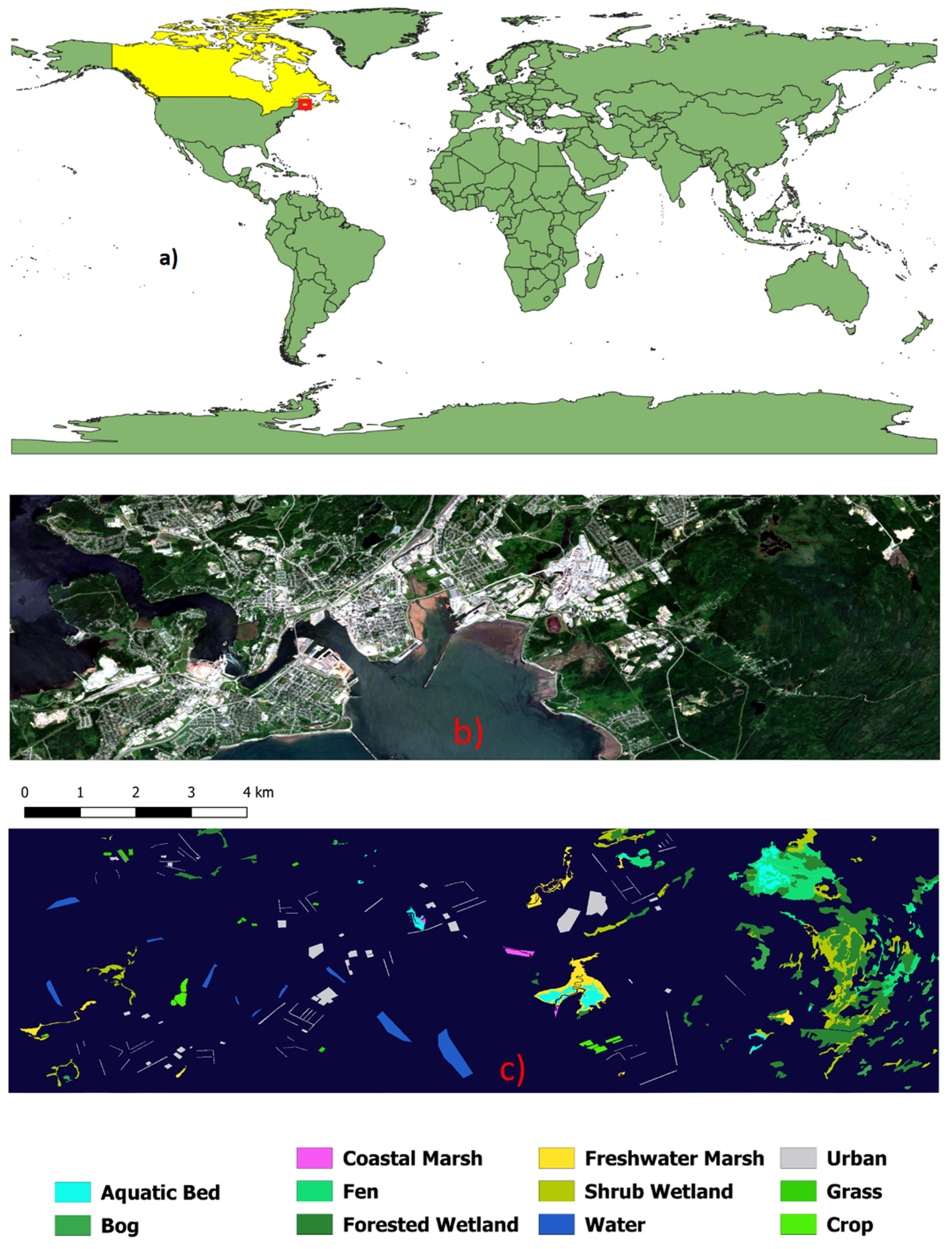
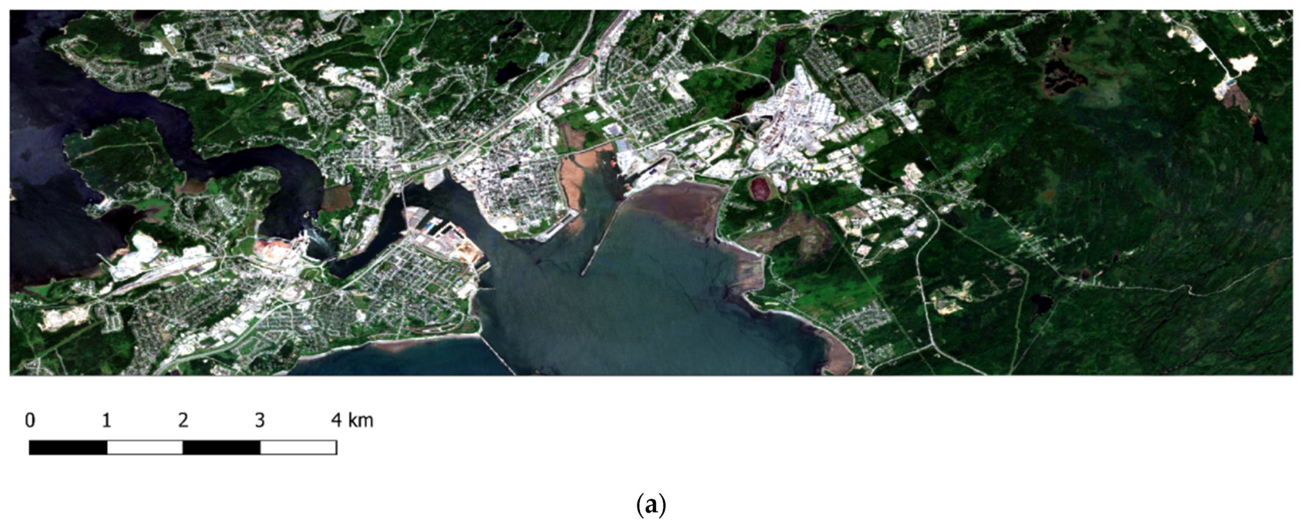
The research area is in Saint John, New Brunswick, Canada, in the province’s south-central region (see Figure 1). Saint John, located on the Bay of Fundy, has a population of over 71,000 people and covers an area of around 326 km². The city is separated by the south-flowing river, while the east side is traversed by the Kennebecasis River, which flows into the Saint John River near Grand Bay. Saint John harbor, located at the junction of the two rivers and the Bay of Fundy, is a deep-water harbor with no ice throughout the year. A humid continental climate prevails throughout the city.

We classified seven types of wetlands using Sentinel-1, Sentinel-2, and LiDAR data, including aquatic bed, bog, coastal marsh, fen, forested wetlands, freshwater marsh, and shrub wetland. Wetland ground truth data was obtained from New Brunswick’s 2021 wetland inventory (http://www.snb.ca/geonb1/e/DC/catalogue-E.asp, accessed on 8 December 2021) (see Figure 2). We manually extracted four additional non-wetland classes of water, urban, grass, and crop through visual interpretation of very high-resolution imagery of Google Earth to avoid over-classification of wetlands in the study area.

Table 1. The number of training and test pixels for the wetland and non-wetlands in the pilot site of Saint John, New Brunswick, Canada.

Class	Training (Pixels)	Test (Pixels)
Aquatic bed	6476	2776
Bog	3833	1643
Coastal marsh	851	364
Fen	15,836	6787
Forested wetland	32,521	13,937
Freshwater marsh	7403	3173
Shrub wetland	15,793	6769
Water	7086	3037
Urban	11,378	4876
Grass	1005	431
Crop	1975	846

shows the total number of training and test data.

Sentinel-1 and Sentinel-2 imagery features, such as normalized backscattering coefficients, spectral bands, and indices, were created in the Google Earth Engine (GEE) code editor (https://code.earthengine.google.com/, accessed on 8 December 2021) as shown in

Table 2. The normalized backscattering coefficients, spectral bands, and indices used in this study ($\mathrm{NDVI}$ = Normalized Difference Vegetation Index, $\mathrm{NDBI}$ = Normalized Difference Build-up Index).

Data	Normalized Backscattering Coefficients/Spectral Bands	Spectral Indices
Sentinel-1	${\sigma }_{VV}^0$$, {\sigma }_{VH}^0$$, {\sigma }_{HH}^0$$, {\sigma }_{HV}^0$
Sentinel-2	B2, B3, B4, B5, B6, B7, B8, B8A, B11, B12	$\mathrm{NDVI}=\frac{\left(\mathrm{NIR}-\mathrm{R}\right)}{\left(\mathrm{NIR}+\mathrm{R}\right)}$ $\mathrm{NDBI}=\frac{\left(\mathrm{SWIR}-\mathrm{NIR}\right)}{\left(\mathrm{SWIR}+\mathrm{NIR}\right)}$

. As satellite images are pre-processed in GEE, we did not perform any image pre-processing for Sentinel-1 and Sentinel-2 imagery. We used Las Tools (https://rapidlasso.com/lastools/, accessed on 8 December 2021) with QGIS 3.16.7 software to produce a DEM from LiDAR data to increase the coastal wetland classification accuracy in the Saint John pilot site. The DEM was resampled into 10 m before being stacked with Sentinel-1 and Sentinel-2 images with the use of the raster calculator in QGIS 3.16.7 software. It is worth noting that the LiDAR data had a point density of six points per square meter.

3.2. Methods

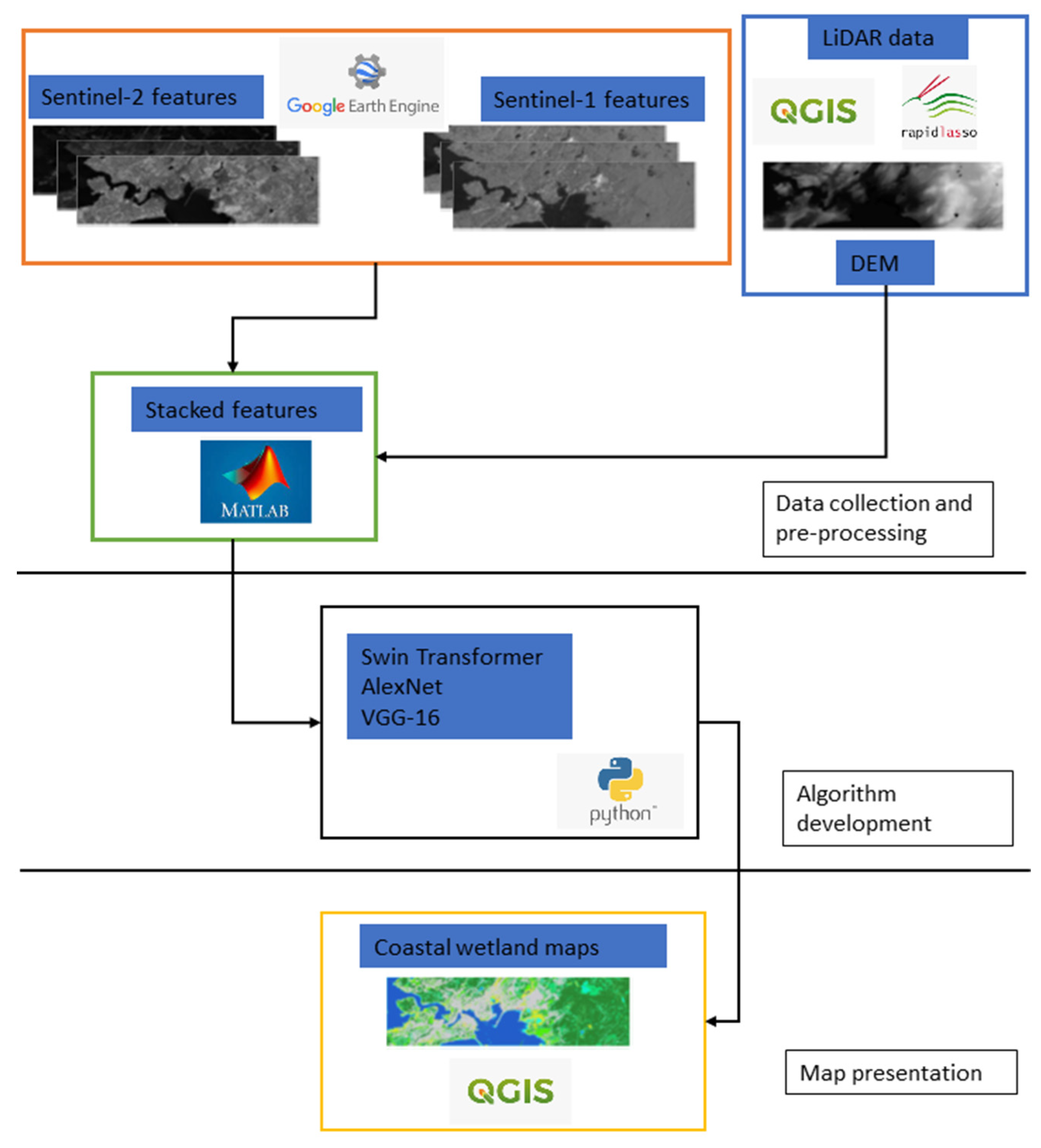
The flowchart of this research is shown in Figure 2. As seen in Figure 2, Sentinel-1 and Sentinel-2 features are extracted from GEE, while DEM is generated from LiDAR data with the use of QGIS 3.16.7 software and the LAS tool. Afterward, extracted features are stacked using the MATLAB programming language. Then, the Python programming language is used to develop deep learning classifiers of Swin Transformer, AlexNet, and VGG-16, followed by classification map presentation in QGIS 3.16.7 software.

3.2.1. VGG-16

As seen in Figure 3, this 16-layer network with about 138 million parameters was trained and tested on the ImageNet dataset by the University of Oxford’s Visual Geometry Group. The original VGG-16 model architecture is made up of 3 by 3 kernel-sized filters that allow the network to learn increasingly complicated features by increasing the depth of the network [55]. There are 13 convolutional and 3 fully connected layers in the architecture of the VGG-16 DCNN network, as seen in Figure 3. It is worth highlighting that there are five max-pooling layers in the VGG-16 network.

3.2.2. AlexNet

Krizhevsky [56] introduced AlexNet as a classic and better-performing network structure of CNNs in a recognizing duty competition called ImageNet. Introducing the activation function of ReLU and revolutionary dropout procedures helped avoid the over-fitting issue. The goal was to improve AlexNet’s validation accuracy, as well as its generalization capabilities. AlexNet’s concept offered ample space for engineering scientific research while also opening up a new window for upcoming artificial intelligence technology. Figure 4 depicts the AlexNet architecture. There are six convolutional layers in AlexNet architecture. The first and second convolutional layers have kernel sizes of 11 by 11 and 5 by 5, while the remaining convolutional layers have kernel sizes of 3 by 3. In the architecture of AlexNet, there are three fully connected layers, as seen in Figure 4.

3.2.3. Proposed Swin Transformer Classifier

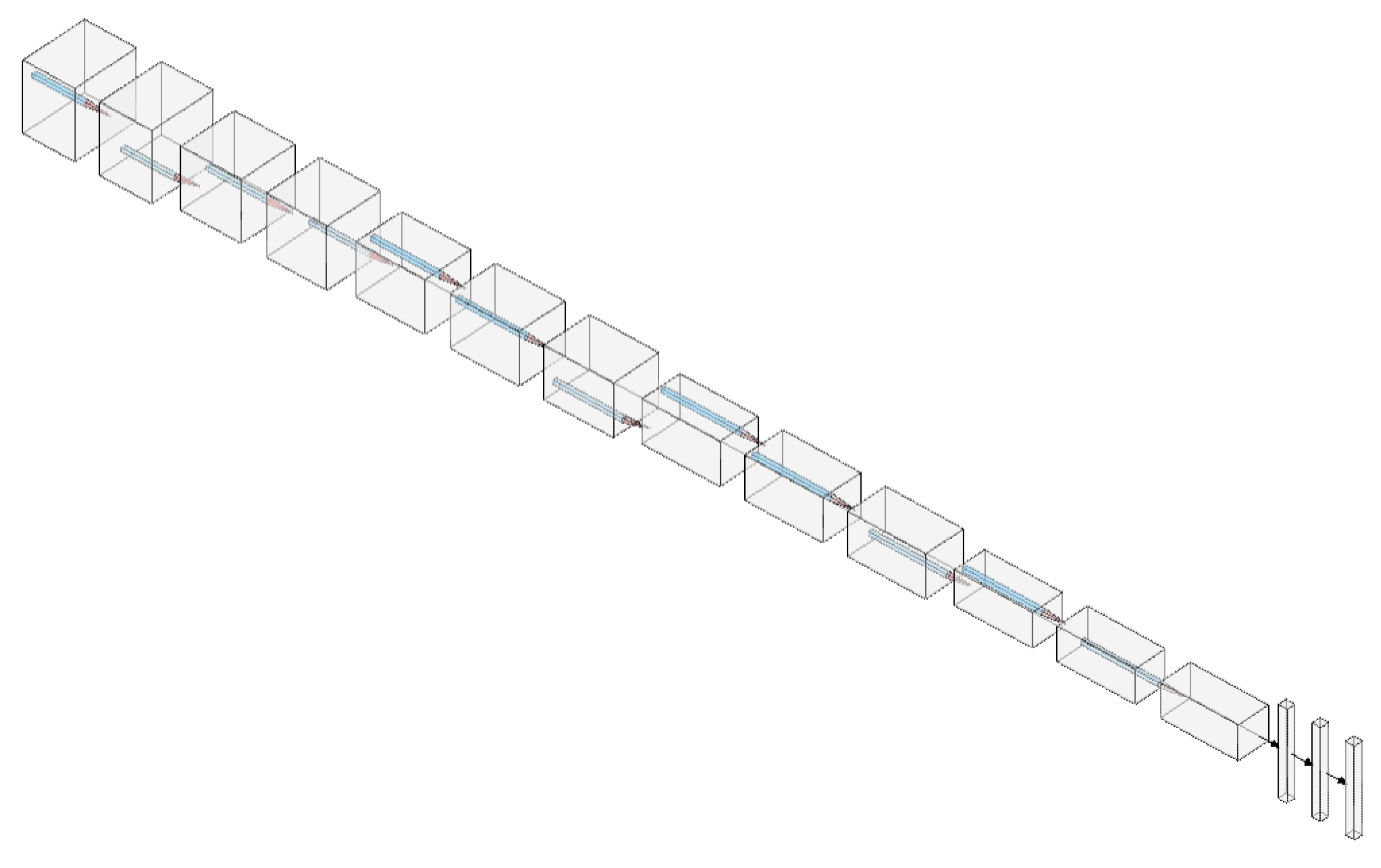
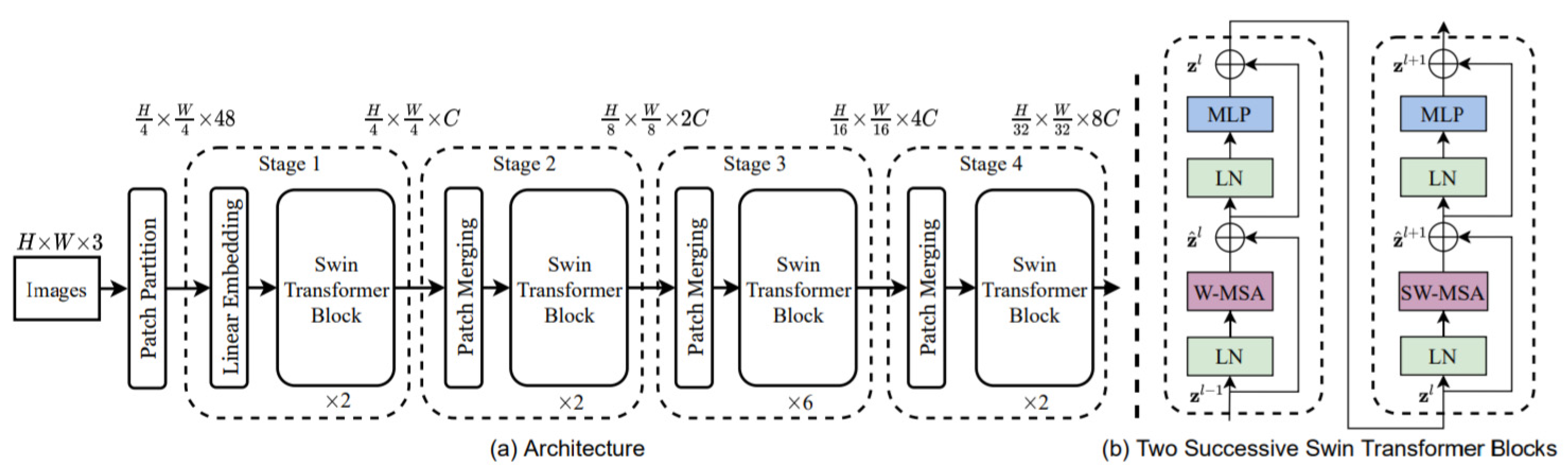
Differences between language and vision, such as large differences in the scale of visual entities and the high resolution of pixels in images compared to words in texts, make it difficult to apply transformer models from language to vision. However, the Swin Transformer presented a hierarchical transformer whose representation is computed using shifted windows [57] (see Figure 5). The shifted windowing technique enhances efficiency by limiting self-attention computation to non-overlapping local windows while allowing for cross-window connectivity. This hierarchical architecture has a linear computing complexity as image size increases and can predict at different scales. The properties of the Swin Trans-former make it suited for a wide range of vision applications, including remote sensing image classification.

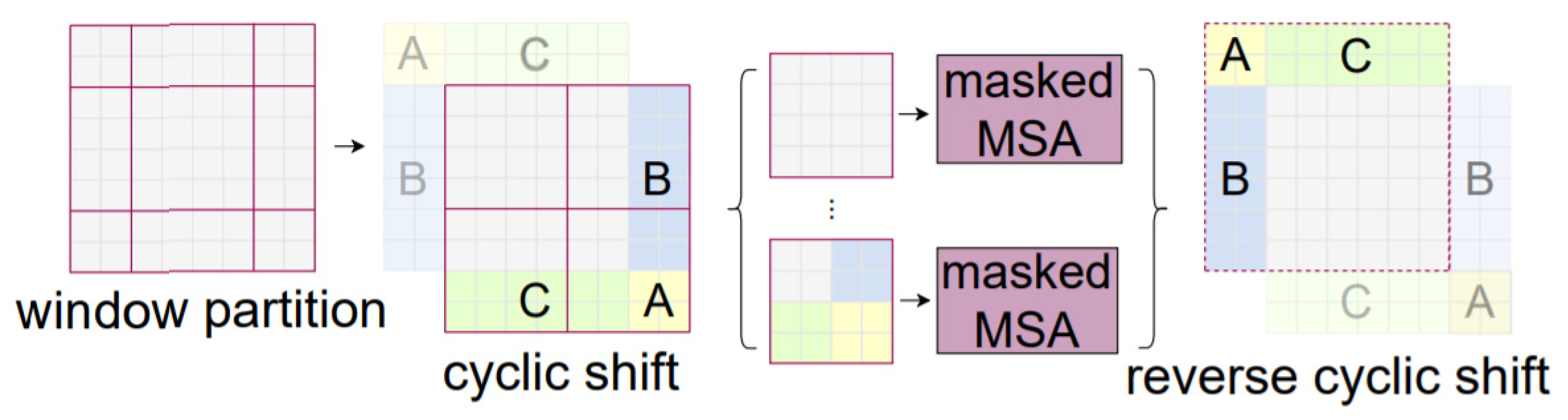
Because it introduces links between neighboring non-overlapping windows in the previous layer, the shifted window partitioning technique is successful in image classification, object detection, and semantic segmentation (see Figure 6) (for more information, refer to Liu et al. [57]).

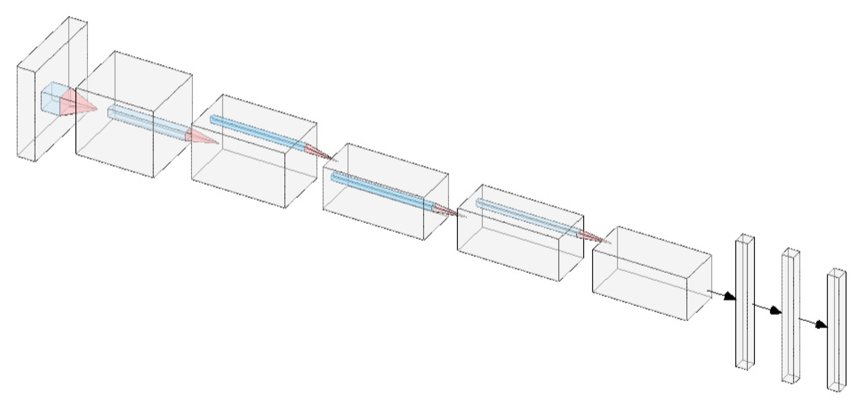
Instead of using two multi-head self-attention modules, we experimentally used four consecutive Swin Transformers in the modified version of the proposed complex wetland classification algorithm. The four Swin Transformer blocks are computed consecutively using the shifting window partitioning method (see Equations (1)–(8)):

$${\hat{\mathrm{z}}}^{\mathrm{l}}=\mathrm{WMSA}\left(\mathrm{LN}({\mathrm{z}}^{\mathrm{l}-1})\right)+{\mathrm{z}}^{\mathrm{l}-1}$$

(1)

$${\mathrm{z}}^{\mathrm{l}}=\mathrm{MLP}\left(\mathrm{LN}({\hat{\mathrm{z}}}^{\mathrm{l}})\right)+{\hat{\mathrm{z}}}^{\mathrm{l}}$$

(2)

$${\hat{\mathrm{z}}}^{\mathrm{l}+1}=\mathrm{SWMSA}\left(\mathrm{LN}({\mathrm{z}}^{\mathrm{l}})\right)+{\mathrm{z}}^{\mathrm{l}}$$

(3)

$${\mathrm{z}}^{\mathrm{l}+1}=\mathrm{MLP}\left(\mathrm{LN}({\hat{\mathrm{z}}}^{\mathrm{l}+1})\right)+{\hat{\mathrm{z}}}^{\mathrm{l}+1 }$$

(4)

$${\hat{\mathrm{z}}}^{\mathrm{l}+2}=\mathrm{WMSA}2\left(\mathrm{LN}({\mathrm{z}}^{\mathrm{l}+1})\right)+{\mathrm{z}}^{\mathrm{l}+1}$$

(5)

$${\mathrm{z}}^{\mathrm{l}+2}=\mathrm{MLP}\left(\mathrm{LN}({\hat{\mathrm{z}}}^{\mathrm{l}+2})\right)+{\hat{\mathrm{z}}}^{\mathrm{l}+2}$$

(6)

$${\hat{\mathrm{z}}}^{\mathrm{l}+3}=\mathrm{SWMSA}2\left(\mathrm{LN}({\mathrm{z}}^{\mathrm{l}+2})\right)+{\mathrm{z}}^{\mathrm{l}+2}$$

(7)

$${\mathrm{z}}^{\mathrm{l}+3}=\mathrm{MLP}\left(\mathrm{LN}({\hat{\mathrm{z}}}^{\mathrm{l}+3})\right)+{\hat{\mathrm{z}}}^{\mathrm{l}+3 }$$

(8)

where ${\hat{\mathrm{z}}}^{\mathrm{l}}$ and ${\mathrm{z}}^{\mathrm{l}}$ present the outputs of (S)W-MSA(2) and $\mathrm{MLP}$ module of block $\mathrm{l}$, respectively. SW-MSA(2) and W-MSA(2) are multi-head self-attention modules with shifted windowing and regular settings, respectively.

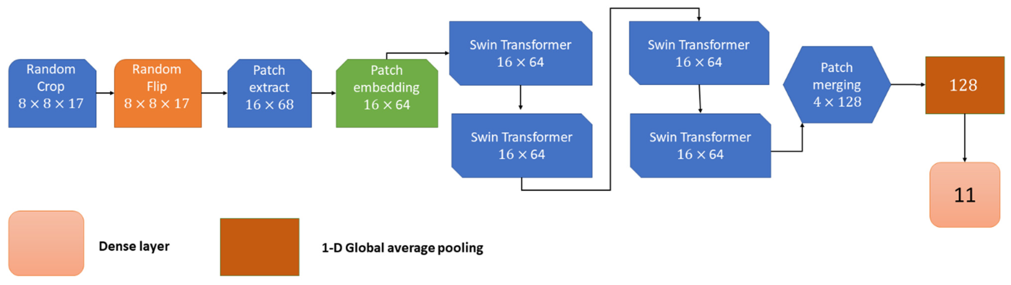
The architecture of the proposed Swin Transformer model for complex coastline classification is presented in Figure 7. It is worth noting that the Swin Transformer model’s first two layers (random crop and random flip) are data augmentation approaches. In the patch extract layer, image patches of 2 by 2 were taken from input images and turned into linear features of size 68 ($17\times 4$), yielding an output feature of 16 by 68. The output feature in the patch embedding layer was features of size 16 by 64 because we used an embedding dimension of 64. Image patches are converted (i.e., translated) into vector data at the embedding layer, which is then employed in transformers. The output vectors are then sent through the Swin Transformers. The Swin Transformer’s output features are then merged using a patch merging layer, yielding an output feature of 4 by 128, which is then followed by a 1-D global average pooling with a size of 128. The last layer is a dense layer with a size of 11.

In the Swin Transformer, we used patch size, dropout rate, number of attention heads, embedding dimension, number of multi-layer perceptrons, and shift size of $2\times 2$, 0.04, 8, 64, 256, and 1, respectively.

3.2.4. Accuracy Assessment

Coastal wetland classification results were quantitatively assessed in terms of the average accuracy, recall, precision, F1-score, and overall accuracy metrics (Equations (9)–(13)).

$$\mathrm{Precision}=\frac{\mathrm{True} \mathrm{positive}}{\left(\mathrm{True} \mathrm{positive}+\mathrm{False} \mathrm{positive}\right)}$$

(9)

$$\mathrm{Recall}=\frac{\mathrm{True} \mathrm{positive}}{\left(\mathrm{True} \mathrm{positive}+\mathrm{False} \mathrm{negative}\right)}$$

(10)

$$\mathrm{Ovrall} \mathrm{Accuracy}=\frac{\left(\mathrm{True} \mathrm{positive}+\mathrm{True} \mathrm{Negative}\right)}{\mathrm{Total} \mathrm{number} \mathrm{of} \mathrm{pixels}}\times 100$$

(11)

$$\mathrm{F}1-\mathrm{score}=2\ast \frac{\mathrm{Precision}\ast \mathrm{Recall}}{\mathrm{Precision}+ \mathrm{Recall}}$$

(12)

$$\mathrm{Average} \mathrm{Accuracy}=\frac{{{\displaystyle \sum }}_{\mathrm{i}=1}^{\mathrm{n}}{\mathrm{Recall}}_{\mathrm{i}}}{\mathrm{n}}$$

(13)

Precision, recall, and F1-score metrics are statistical metrics that present the performance of each classifier for the recognition of wetlands and non-wetlands per class. Average accuracy is the mean of recalls, while overall accuracy is the most used overall performance of machine learning classifiers for the classification of different remote sensing features. The issue with the overall accuracy metric is that in wetland classification tasks, there are much higher ground truth data for non-wetlands than wetland classes [47], resulting in a high level of overall accuracy even though per-class accuracies in wetlands can be much lower than in non-wetlands. It is worth highlighting that we divided our ground truth data into 70 percent training and 30 percent test samples using a stratified random sampling technique implemented in Python programming language with the use of the sklearn library.

4. Results

4.1. Statistical Comparison of Developed Models

Comparison results of the complex coastal wetland classification using the modified Swin Transformer, AlexNet, and VGG-16 are shown in

Table 3. Results of the proposed multi-model compared to other classifiers in terms of average accuracy, precision, F1-score, and recall (AB = Aquatic bed, BO = Bog, CM = Coastal marsh, FE = Fen, FM = Freshwater marsh, FW = Forested wetland, SB = Shrub wetland, W = Water, U = Urban, G = Grass, C = Crop, AA = Average accuracy, OA = Overall accuracy).

Model	AB	BO	CM	FE	FW	FM	SB	W	U	G	C	AA (%)	OA (%)
Swin Transformer												81.48	82.52
Precision	0.85	0.72	0.87	0.80	0.82	0.81	0.75	0.94	0.93	0.73	0.89
Recall	0.80	0.75	0.52	0.75	0.86	0.87	0.68	0.99	0.95	0.93	0.87
F-1 score	0.82	0.73	0.65	0.78	0.84	0.84	0.71	0.97	0.94	0.82	0.88
AlexNet												67.18	68.81
Precision	0.73	0.28	0.61	0.55	0.86	0.71	0.54	0.98	0.76	0.59	0.88
Recall	0.86	0.55	0.44	0.72	0.62	0.78	0.40	1	0.99	0.50	0.52
F-1 score	0.79	0.37	0.51	0.62	0.72	0.74	0.46	0.99	0.86	0.54	0.66
VGG-16												37.20	54.48
Precision	0.41	0.21	0.12	0.68	0.50	0.47	0.35	1	0.99	0.96	0.54
Recall	0.48	0.03	0.0	0.08	0.97	0.88	0.09	0.52	0.76	0.26	0.02
F-1 score	0.44	0.05	0.01	0.15	0.66	0.61	0.14	0.68	0.86	0.41	0.03

. Based on the achieved results, the proposed classifier had the best performance over both deep CNN networks of AlexNet and VGG-16. In terms of average accuracy, the proposed Swin Transformer algorithm outperformed the AlexNet and VGG-16 techniques by 14.3% and 44.28%, respectively. The proposed classifier obtained F1-scores of 0.65, 0.71, 0.73, 0.78, 0.82, 0.84, and 0.84 to recognize coastal marsh, shrub, bog, fen, aquatic bed, forested wetland, and freshwater marsh, respectively. The VGG-16 deep CNN classifier obtained the least performance. The very deep structure of VGG-16 and its higher number of hyper-parameters over the AlexNet and the proposed Swin Transformer network can be explained as the possible reasons behind the lower performance of the VGG-16 network. The Swin Transformer improved the F1-scores of wetland classes of bog, shrub, fen, coastal marsh, forested wetland, freshwater marsh, and aquatic bed by 36%, 25%, 16%, 14%, 12%, 10%, and 3%, respectively, compared to the AlexNet classifier. On the other hand, the F1-scores of shrub, bog, coastal marsh, fen, aquatic bed, freshwater marsh, and forested wetlands obtained by the VGG-16 DCNN algorithm were improved by 70%, 68%, 64%, 63%, 38%, 23%, and 18%, respectively, by the proposed Swin Transformer classifier (see Table 3).

As seen in

Table 4. Confusion matrix of the VGG-16 (AB = Aquatic bed, BO = Bog, CM = Coastal marsh, FE = Fen, FM = Freshwater marsh, FW = Forested wetland, SB = Shrub wetland, W = Water, U = Urban, G = Grass, C = Crop).

Model	AB	BO	CM	FE	FW	FM	SB	W	U	G	C
VGG-16
AB	1329	0	0	229	90	1054	70	0	3	1	0
BO	0	49	0	16	1348	129	101	0	0	0	0
CM	32	0	1	0	0	323	8	0	0	0	0
FE	19	0	0	574	5722	194	278	0	0	0	0
FW	0	1	0	0	13,571	118	241	0	6	0	0
FM	11	1	0	9	295	2778	79	0	0	0	0
SB	8	139	0	1	5460	545	604	0	12	0	0
W	1458	0	0	0	9	0	0	1570	0	0	0
U	55	33	0	21	389	449	214	0	3715	0	0
G	126	0	7	0	17	62	92	0	2	113	12
C	232	11	0	0	218	288	63	0	16	4	14

,

Table 5. Confusion matrix of the AlexNet (AB = Aquatic bed, BO = Bog, CM = Coastal marsh, FE = Fen, FM = Freshwater marsh, FW = Forested wetland, SB = Shrub wetland, W = Water, U = Urban, G = Grass, C = Crop).

Model	AB	BO	CM	FE	FW	FM	SB	W	U	G	C
AlexNet
AB	2398	1	12	138	1	154	8	24	40	0	0
BO	58	899	0	314	85	101	100	0	86	0	0
CM	76	0	161	0	0	73	1	0	53	0	0
FE	236	657	0	4897	427	197	372	0	1	0	0
FW	147	809	2	1901	8689	273	1683	0	427	0	6
FM	252	17	54	37	3	2464	107	28	198	0	13
SB	102	839	3	1637	920	216	2686	0	337	0	29
W	0	0	0	0	0	0	0	3037	0	0	0
U	29	3	1	1	0	0	14	2	4826	0	0
G	0	0	15	0	0	8	2	0	174	217	15
C	0	0	18	0	0	7	10	0	215	152	444

and

Table 6. Confusion matrix of the Swin Transformer (AB = Aquatic bed, BO = Bog, CM = Coastal marsh, FE = Fen, FM = Freshwater marsh, FW = Forested wetland, SB = Shrub wetland, W = Water, U = Urban, G = Grass, C = Crop).

Model	AB	BO	CM	FE	FW	FM	SB	W	U	G	C
AlexNet
AB	2219	1	0	177	3	143	7	152	54	20	0
BO	1	1225	0	50	249	9	104	0	5	0	0
CM	54	0	188	0	0	72	2	12	33	3	0
FE	99	214	0	5106	968	26	367	0	7	0	0
FW	2	202	1	649	11,960	64	1014	0	36	0	9
FM	201	4	17	25	17	2751	15	26	111	2	4
SB	24	58	5	342	1423	269	4573	0	61	4	10
W	13	0	0	0	0	0	0	3021	2	1	0
U	4	6	5	10	26	45	21	0	4654	45	60
G	4	0	0	0	0	0	0	0	19	401	7
C	2	0	0	0	0	20	0	0	16	73	735

, the proposed Swin Transformer classifier showed the least confusion between wetlands and non-wetlands classes. The highest confusion was between coastal marsh and freshwater marsh. The reason can be attributed to the similar vegetation structure between these two wetland classes. Based on the Swin Transformer algorithm results, there was a high level of confusion between forested wetlands and shrub wetlands. Their similar vegetation types can explain this high level of confusion between these two wetland classes. For instance, forested wetland regions may have woody shrubs, resulting in similar spectral reflectance to shrub wetlands. It should be noted that wetlands have no clear-cut boundaries, and as they may have a common vegetation type, they have similar spectral reflectance in satellite imagery, specifically optical satellite images.

On the other hand, the confusion between wetlands was much higher using the very deep CNN of AlexNet and VGG-16 compared to the Swin Transformer. The highest level of confusion obtained by the AlexNet classifier was between bog and fen, followed by a high level of confusion among shrub and fen wetland classes. It is worth highlighting that bog and fen have a much higher level of similarity in their vegetation structure and types. On the other hand, based on the results of the VGG-16 algorithm, almost all coastal marshes were recognized as freshwater marsh regions, while bog regions were incorrectly classified as forested wetlands. The VGG-16 classifier failed for the recognition of wetlands with less training data (i.e., bog and coastal marsh wetlands). It is worth highlighting that more training data is required to adequately train very deep CNN networks, such as VGG-16 DCNN. However, the proposed Swin Transformer showed that with a small amount of training data, a high level of accuracy could be achieved even in a complex and high-dimensional ecological environment (see Table 4, Table 5 and Table 6).

4.2. Wetland Maps of the Study Area of Saint John City

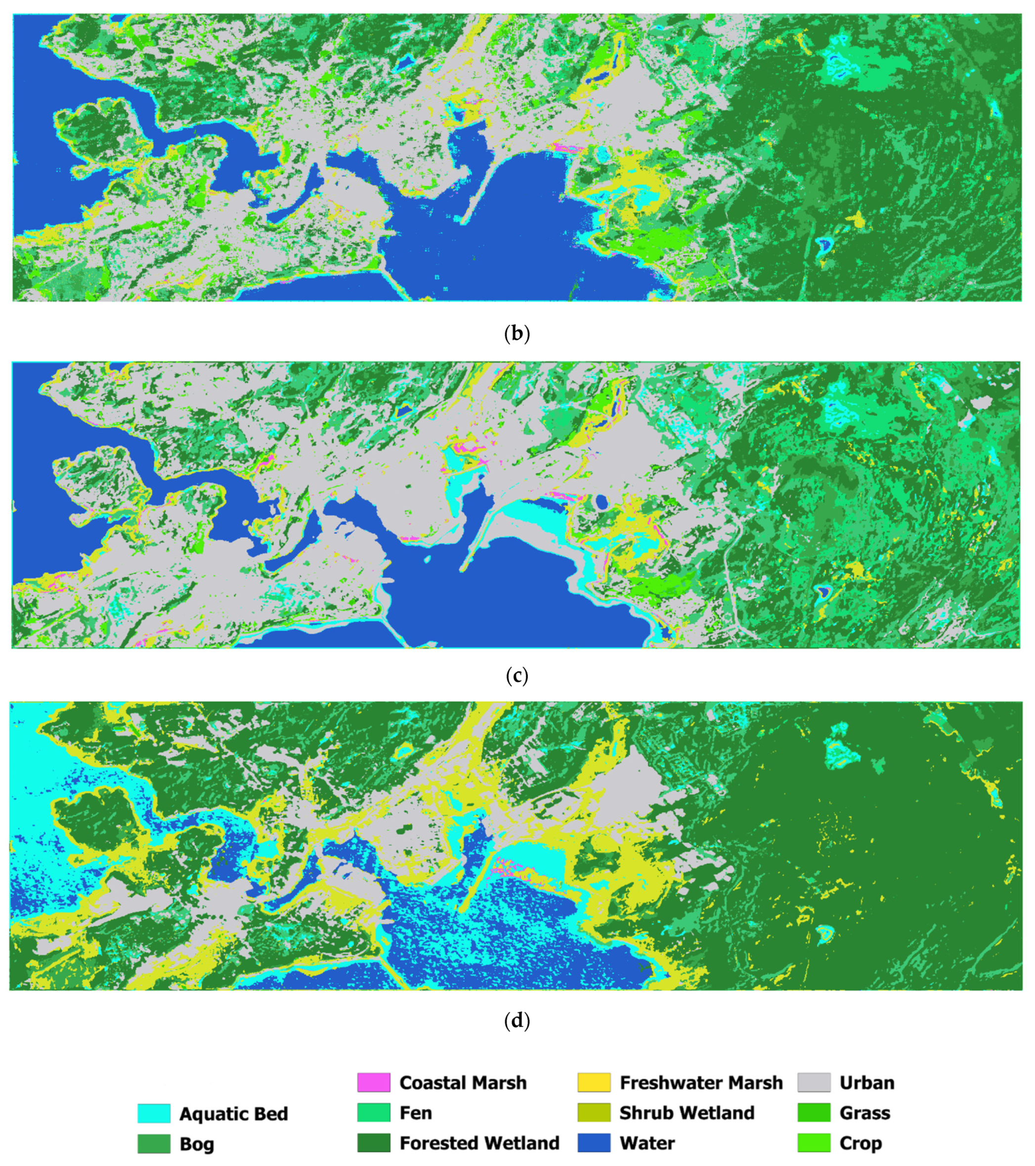
Coastal wetland and non-wetland maps using the proposed Swin Transformer, AlexNet, and VGG-16 are shown in Figure 8. Based on the coastal wetland classification maps, the proposed Swin Transformer classifier obtained the best visual results. For instance, the AlexNet network over-classified urban and shrub areas, while the proposed transformer technique had better results visually and statistically. The coastal wetland map obtained by the VGG-16 network showed over-classification of aquatic bed and forested wetlands, while other wetlands, including bog, fen, and shrub, as well as the non-wetland class of urban were under-classified.

5. Discussion

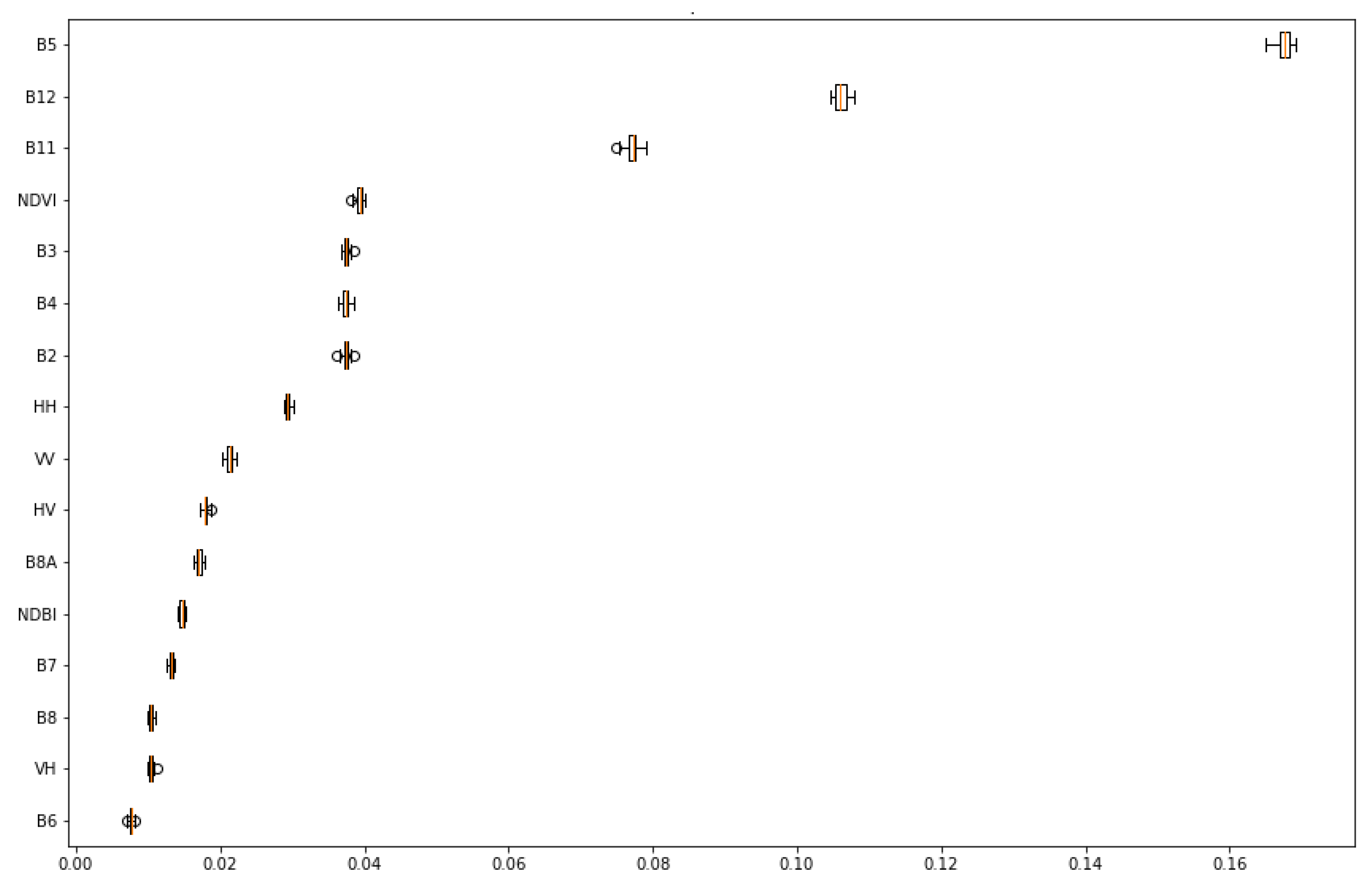
As shown in Figure 9, to fully visualize the magnitude and effectiveness of Sentinel-1 and Sentinel-2 features, the variable importance was assessed. For the spectral analysis, we ran the Random Forest classifier 30 times. Based on the results, Sentinel-2 spectral bands and indices were more effective than Sentinel-1 backscattering features in detecting coastal wetlands in the pilot site of Saint John city, as expected. According to the Gini index for test data prediction, the fifth band of Sentinel-2 (i.e., first vegetation red edge band, B5) was the most influential variable for coastal wetland classification. However, the second vegetation red edge band (i.e., B6) was the least influential variable. Furthermore, the ${\sigma }_{HH}^0$, followed by ${\sigma }_{VV}^0$, backscattering coefficients were Sentinel-1′s most useful features.

Transformers have had a lot of success in solving NLP tasks. A tough challenge in remote sensing complex landscape classification over conventional computer vision image classification is the significantly higher resolution of remote sensing satellite images, despite their high potential for a few computer vision problems. Given that vision transformers have a complexity of $O\left(n^2\right)$ as pixel resolution increases, we chose the Swin Transformer because it has a considerably lower linear complexity of $O\left(n\right)$ as image pixel resolution increases. The Swin Transformer, in other terms, is far more computationally efficient than other visual transformers. For instance, in terms of time, the modified Swin Transformer with 30 min training time was much more efficient over both CNN algorithms of AlexNet and VGG-16 with training times of 60 and 180 min, respectively.

Based on the achieved results, the modified Swin Transformer classifier reached a relatively high average accuracy of 81.48%. As LaRocque et al. [14] discussed, most wetland mapping methods in New Brunswick are based on the manual interpretation of high-resolution imagery. There is not much literature on the use of cutting-edge deep learning methods in the pilot site of Saint John city. LaRocque et al. [14] reported that the RF classifier reached an overall accuracy of 97.67% with the utilization of Landsat 8 OLI, ALOS-1 PALSAR, Sentinel-1, and LiDAR-derived topographic metrics. We cannot precisely compare their obtained results and the results achieved by this study, as our classifiers, the number of training data, and satellite data are different. Based on the achieved results, The Swin Transformer presented its high capability for complex ecological scene classification due to its lower computation cost and much higher classification accuracy than the other two well-known CNN models of AlexNet and VGG-16.

For the implementation of the machine learning algorithms of AlexNet, VGG-16, and the modified Swin Transformer, a Graphical Processing Unit (GPU) of NVIDIA GeForce RTX 2070, a 16 GB Random Access Memory (RAM), and an Intel processor (i.e., i7-10750H Central Processing Unit (CPU) of 2.60 GHz) operating on 64-bit Windows 11 were utilized. It is worth highlighting that all algorithms were developed in the Python TensorFlow library.

6. Conclusions

New solutions and technologies for wetland mapping and monitoring have become crucial because of the considerable benefits that wetland activities deliver to humans and wildlife. Because of their dynamic and varied structure, which lacks clear-cut boundaries and similar vegetation patterns, wetlands are among the most challenging ecosystems to identify. As a result, we investigated the potential of utilizing cutting-edge transformers (i.e., Swin Transformer) for complex landscape classification in the pilot site of Saint John city in New Brunswick, Canada, for the protection and monitoring of coastal wetlands. Based on the achieved results, the modified Swin Transformer presented better results for the classification of the complex environment of Saint John city, visually and statistically. In terms of average accuracy, the proposed Swin Transformer algorithm outperformed the AlexNet and VGG-16 techniques by 14.3% and 44.28%, respectively. Moreover, the proposed transformer machine learning method achieved relatively high F1-scores of 0.65, 0.71, 0.73, 0.78, 0.82, 0.84, and 0.84 for recognizing coastal marsh, shrub, bog, fen, aquatic bed, forested wetland, and freshwater marsh, respectively. In addition, we calculated streamflow of the study area of Saint John city using the LiDAR DEM to investigate the connectivity between wetlands to better understand the potential level of risk over the possible pollution of aquatic and wetland ecosystems. We found a high level of linkage between aquatic and wetland ecosystems in the pilot site that triggers the implementation of future policies over the protection and preservation of coastal wetlands in Saint John city.

References

- Davidson, N.C. The Ramsar Convention on Wetlands. In The Wetland Book I: Structure and Function, Management and Methods; Springer: Dordrecht, The Netherlands, 2016. [Google Scholar]
- Jamali, A.; Mahdianpari, M.; Brisco, B.; Granger, J.; Mohammadimanesh, F.; Salehi, B. Wetland Mapping Using Multi-Spectral Satellite Imagery and Deep Convolutional Neural Networks: A Case Study in Newfoundland and Labrador, Canada. Can. J. Remote Sens. 2021, 47, 243–260. [Google Scholar] [CrossRef]
- Mahdianpari, M.; Salehi, B.; Mohammadimanesh, F.; Homayouni, S.; Gill, E. The First Wetland Inventory Map of Newfoundland at a Spatial Resolution of 10 m Using Sentinel-1 and Sentinel-2 Data on the Google Earth Engine Cloud Computing Platform. Remote Sens. 2019, 11, 43. [Google Scholar] [CrossRef] [Green Version]
- Mitsch, W.J.; Bernal, B.; Hernandez, M.E. Ecosystem Services of Wetlands. Int. J. Biodivers. Sci. Ecosyst. Serv. Manag. 2015, 11, 1–4. [Google Scholar] [CrossRef] [Green Version]
- van Asselen, S.; Verburg, P.H.; Vermaat, J.E.; Janse, J.H. Drivers of Wetland Conversion: A Global Meta-Analysis. PLoS ONE 2013, 8, e81292. [Google Scholar] [CrossRef] [Green Version]
- Mahdavi, S.; Salehi, B.; Granger, J.; Amani, M.; Brisco, B.; Huang, W. Remote Sensing for Wetland Classification: A Comprehensive Review. GIScience Remote Sens. 2018, 55, 623–658. [Google Scholar] [CrossRef]
- Guo, M.; Li, J.; Sheng, C.; Xu, J.; Wu, L. A Review of Wetland Remote Sensing. Sensors 2017, 17, 777. [Google Scholar] [CrossRef] [Green Version]
- Jamali, A.; Mahdianpari, M.; Brisco, B.; Granger, J.; Mohammadimanesh, F.; Salehi, B. Deep Forest Classifier for Wetland Mapping Using the Combination of Sentinel-1 and Sentinel-2 Data. GISci. Remote Sens. 2021, 58, 1072–1089. [Google Scholar] [CrossRef]
- Jamali, A.; Mahdianpari, M.; Brisco, B.; Granger, J.; Mohammadimanesh, F.; Salehi, B. Comparing Solo Versus Ensemble Convolutional Neural Networks for Wetland Classification Using Multi-Spectral Satellite Imagery. Remote Sens. 2021, 13, 2046. [Google Scholar] [CrossRef]
- Costanza, R.; de Groot, R.; Sutton, P.; van der Ploeg, S.; Anderson, S.J.; Kubiszewski, I.; Farber, S.; Turner, R.K. Changes in the Global Value of Ecosystem Services. Glob. Environ. Chang. 2014, 26, 152–158. [Google Scholar] [CrossRef]
- De Groot, R.; Brander, L.; van der Ploeg, S.; Costanza, R.; Bernard, F.; Braat, L.; Christie, M.; Crossman, N.; Ghermandi, A.; Hein, L.; et al. Global Estimates of the Value of Ecosystems and Their Services in Monetary Units. Ecosyst. Serv. 2012, 1, 50–61. [Google Scholar] [CrossRef]
- Zedler, J.B.; Kercher, S. Causes and Consequences of Invasive Plants in Wetlands: Opportunities, Opportunists, and Outcomes. Crit. Rev. Plant Sci. 2004, 23, 431–452. [Google Scholar] [CrossRef]
- Perillo, G.; Wolanski, E.; Cahoon, D.R.; Hopkinson, C.S. Coastal Wetlands: And Integrated Ecosystem Approach; Elsevier: Oxford, UK, 2018. [Google Scholar]
- LaRocque, A.; Phiri, C.; Leblon, B.; Pirotti, F.; Connor, K.; Hanson, A. Wetland Mapping with Landsat 8 OLI, Sentinel-1, ALOS-1 PALSAR, and LiDAR Data in Southern New Brunswick, Canada. Remote Sens. 2020, 12, 2095. [Google Scholar] [CrossRef]
- Mahdianpari, M.; Salehi, B.; Mohammadimanesh, F.; Motagh, M. Random Forest Wetland Classification Using ALOS-2 L-Band, RADARSAT-2 C-Band, and TerraSAR-X Imagery. ISPRS J. Photogramm. Remote Sens. 2017, 130, 13–31. [Google Scholar] [CrossRef]
- DeLancey, E.R.; Simms, J.F.; Mahdianpari, M.; Brisco, B.; Mahoney, C.; Kariyeva, J. Comparing Deep Learning and Shallow Learning for Large-Scale Wetland Classification in Alberta, Canada. Remote Sens. 2020, 12, 2. [Google Scholar] [CrossRef] [Green Version]
- Mohammadimanesh, F.; Salehi, B.; Mahdianpari, M.; Brisco, B.; Gill, E. Full and Simulated Compact Polarimetry Sar Responses to Canadian Wetlands: Separability Analysis and Classification. Remote Sens. 2019, 11, 516. [Google Scholar] [CrossRef] [Green Version]
- Kentsch, S.; Cabezas, M.; Tomhave, L.; Groß, J.; Burkhard, B.; Lopez Caceres, M.L.; Waki, K.; Diez, Y. Analysis of UAV-Acquired Wetland Orthomosaics Using GIS, Computer Vision, Computational Topology and Deep Learning. Sensors 2021, 21, 471. [Google Scholar] [CrossRef]
- Mao, D.; Wang, Z.; Du, B.; Li, L.; Tian, Y.; Jia, M.; Zeng, Y.; Song, K.; Jiang, M.; Wang, Y. National Wetland Mapping in China: A New Product Resulting from Object-Based and Hierarchical Classification of Landsat 8 OLI Images. ISPRS J. Photogramm. Remote Sens. 2020, 164, 11–25. [Google Scholar] [CrossRef]
- Amani, M.; Brisco, B.; Mahdavi, S.; Ghorbanian, A.; Moghimi, A.; DeLancey, E.R.; Merchant, M.; Jahncke, R.; Fedorchuk, L.; Mui, A.; et al. Evaluation of the Landsat-Based Canadian Wetland Inventory Map Using Multiple Sources: Challenges of Large-Scale Wetland Classification Using Remote Sensing. IEEE J. Sel. Top. Appl. Earth Obs. Remote Sens. 2021, 14, 32–52. [Google Scholar] [CrossRef]
- Belgiu, M.; Drăguţ, L. Random Forest in Remote Sensing: A Review of Applications and Future Directions. ISPRS J. Photogramm. Remote Sens. 2016, 114, 24–31. [Google Scholar] [CrossRef]
- Camargo, F.F.; Sano, E.E.; Almeida, C.M.; Mura, J.C.; Almeida, T. A Comparative Assessment of Machine-Learning Techniques for Land Use and Land Cover Classification of the Brazilian Tropical Savanna Using ALOS-2/PALSAR-2 Polarimetric Images. Remote Sens. 2019, 11, 1600. [Google Scholar] [CrossRef] [Green Version]
- Collins, L.; Griffioen, P.; Newell, G.; Mellor, A. The Utility of Random Forests for Wildfire Severity Mapping. Remote Sens. Environ. 2018, 216, 374–384. [Google Scholar] [CrossRef]
- Collins, L.; McCarthy, G.; Mellor, A.; Newell, G.; Smith, L. Training Data Requirements for Fire Severity Mapping Using Landsat Imagery and Random Forest. Remote Sens. Environ. 2020, 245, 111839. [Google Scholar] [CrossRef]
- Congalton, R.; Green, K. Assessing the Accuracy of Remotely Sensed Data: Principles and Practices; CRC Press: Boca Raton, FL, USA, 2009. [Google Scholar]
- Bazi, Y.; Bashmal, L.; Rahhal, M.M.A.; Dayil, R.A.; Ajlan, N.A. Vision Transformers for Remote Sensing Image Classification. Remote Sens. 2021, 13, 516. [Google Scholar] [CrossRef]
- He, J.; Zhao, L.; Yang, H.; Zhang, M.; Li, W. HSI-BERT: Hyperspectral Image Classification Using the Bidirectional Encoder Representation from Transformers. IEEE Trans. Geosci. Remote Sens. 2020, 58, 165–178. [Google Scholar] [CrossRef]
- Hong, D.; Han, Z.; Yao, J.; Gao, L.; Zhang, B.; Plaza, A.; Chanussot, J. SpectralFormer: Rethinking Hyperspectral Image Classification with Transformers. IEEE Trans. Geosci. Remote Sens. 2021. [Google Scholar] [CrossRef]
- Azeez, N.; Yahya, W.; Al-Taie, I.; Basbrain, A.; Clark, A. Regional Agricultural Land Classification Based on Random Forest (RF), Decision Tree, and SVMs Techniques; Springer: Berlin/Heidelberg, Germany, 2020; pp. 73–81. [Google Scholar]
- Berhane, T.M.; Lane, C.R.; Wu, Q.; Autrey, B.C.; Anenkhonov, O.A.; Chepinoga, V.V.; Liu, H. Decision-Tree, Rule-Based, and Random Forest Classification of High-Resolution Multispectral Imagery for Wetland Mapping and Inventory. Remote Sens. 2018, 10, 580. [Google Scholar] [CrossRef] [Green Version]
- Bennett, K.P. Global Tree Optimization: A Non-Greedy Decision Tree Algorithm. Comput. Sci. Stat. 1995, 26, 156. [Google Scholar]
- Ebrahimy, H.; Mirbagheri, B.; Matkan, A.A.; Azadbakht, M. Per-Pixel Land Cover Accuracy Prediction: A Random Forest-Based Method with Limited Reference Sample Data. ISPRS J. Photogramm. Remote Sens. 2021, 172, 17–27. [Google Scholar] [CrossRef]
- Cortes, C.; Vapnik, V. Support-Vector Networks. Mach. Learn. 1995, 20, 273–297. [Google Scholar] [CrossRef]
- Sheykhmousa, M.; Mahdianpari, M.; Ghanbari, H.; Mohammadimanesh, F.; Ghamisi, P.; Homayouni, S. Support Vector Machine Versus Random Forest for Remote Sensing Image Classification: A Meta-Analysis and Systematic Review. IEEE J. Sel. Top. Appl. Earth Obs. Remote Sens. 2020, 13, 6308–6325. [Google Scholar] [CrossRef]
- Shao, Y.; Lunetta, R.S. Comparison of Support Vector Machine, Neural Network, and CART Algorithms for the Land-Cover Classification Using Limited Training Data Points. ISPRS J. Photogramm. Remote Sens 2012, 70, 78–87. [Google Scholar] [CrossRef]
- Alhichri, H.; Alswayed, A.S.; Bazi, Y.; Ammour, N.; Alajlan, N.A. Classification of Remote Sensing Images Using EfficientNet-B3 CNN Model with Attention. IEEE Access 2021, 9, 14078–14094. [Google Scholar] [CrossRef]
- Zhang, C.; Pan, X.; Li, H.; Gardiner, A.; Sargent, I.; Hare, J.; Atkinson, P.M. A Hybrid MLP-CNN Classifier for Very Fine Resolution Remotely Sensed Image Classification. ISPRS J. Photogramm. Remote Sens. 2018, 140, 133–144. [Google Scholar] [CrossRef] [Green Version]
- Kattenborn, T.; Leitloff, J.; Schiefer, F.; Hinz, S. Review on Convolutional Neural Networks (CNN) in Vegetation Remote Sensing. ISPRS J. Photogramm. Remote Sens. 2021, 173, 24–49. [Google Scholar] [CrossRef]
- Liang, J.; Deng, Y.; Zeng, D. A Deep Neural Network Combined CNN and GCN for Remote Sensing Scene Classification. IEEE J. Sel. Top. Appl. Earth Obs. Remote Sens. 2020, 13, 4325–4338. [Google Scholar] [CrossRef]
- He, K.; Zhang, X.; Ren, S.; Sun, J. Deep Residual Learning for Image Recognition. In Proceedings of the IEEE Conference on Computer Vision and Pattern Recognition (CVPR), Las Vegas, NV, USA, 26 June–1 July 2016; pp. 770–778. [Google Scholar]
- Huang, G.; Liu, Z.; Van Der Maaten, L.; Weinberger, K.Q. Densely Connected Convolutional Networks. In Proceedings of the IEEE Conference on Computer Vision and Pattern Recognition (CVPR), Honolulu, HI, USA, 21–26 July 2017; pp. 4700–4708. [Google Scholar]
- Xie, S.; Girshick, R.; Dollar, P.; Tu, Z.; He, K. Aggregated residual Transformations for Deep Neural Networks. In Proceedings of the IEEE Conference on Computer Vision and Pattern Recognition (CVPR), Las Vegas, NV, USA, 26 June–1 July 2016. [Google Scholar]
- Cao, J.; Cui, H.; Zhang, Q.; Zhang, Z. Ancient Mural Classification Method Based on Improved AlexNet Network. Stud. Conserv. 2020, 65, 411–423. [Google Scholar] [CrossRef]
- Vaswani, A.; Shazeer, N.; Parmar, N.; Uszkoreit, J.; Jones, L.; Gomez, A.N.; Kaiser, Ł.; Polosukhin, I. Attention Is All You Need. In Advances in Neural Information Processing Systems; The MIT Press: Cambridge, MA, USA, 2017; pp. 5998–6008. [Google Scholar]
- Amani, M.; Salehi, B.; Mahdavi, S.; Brisco, B. Spectral Analysis of Wetlands Using Multi-Source Optical Satellite Imagery. ISPRS J. Photogramm. Remote Sens. 2018, 144, 119–136. [Google Scholar] [CrossRef]
- Amani, M.; Mahdavi, S.; Berard, O. Supervised Wetland Classification Using High Spatial Resolution Optical, SAR, and LiDAR Imagery. J. Appl. Remote Sens. 2020, 14, 024502. [Google Scholar] [CrossRef]
- Jamali, A.; Mahdianpari, M.; Mohammadimanesh, F.; Brisco, B.; Salehi, B. A Synergic Use of Sentinel-1 and Sentinel-2 Imagery for Complex Wetland Classification Using Generative Adversarial Network (GAN) Scheme. Water 2021, 13, 3601. [Google Scholar] [CrossRef]
- Jamali, A.; Mahdianpari, M. A Cloud-Based Framework for Large-Scale Monitoring of Ocean Plastics Using Multi-Spectral Satellite Imagery and Generative Adversarial Network. Water 2021, 13, 2553. [Google Scholar] [CrossRef]
- Goodfellow, I.; Pouget-Abadie, J.; Mirza, M.; Xu, B.; Warde-Farley, D.; Ozair, S.; Courville, A.; Bengio, Y. Generative Adversarial Nets. In Advances in Neural Information Processing Systems; The MIT Press: Cambridge, MA, USA, 2014; Volume 27, pp. 2672–2680. [Google Scholar]
- Zhu, L.; Chen, Y.; Ghamisi, P.; Benediktsson, J.A. Generative Adversarial Networks for Hyperspectral Image Classification. IEEE Trans. Geosci. Remote Sens. 2018, 56, 5046–5063. [Google Scholar] [CrossRef]
- NAudebert; le Saux, B.; Lefevre, S. Generative Adversarial Networks for Realistic Synthesis of Hyperspectral Samples. In Proceedings of the IGARSS 2018–2018 IEEE International Geoscience and Remote Sensing Symposium, Valencia, Spain, 22–27 July 2018; pp. 4359–4362. [Google Scholar]
- Granger, J.E.; Mahdianpari, M.; Puestow, T.; Warren, S.; Mohammadimanesh, F.; Salehi, B.; Brisco, B. Object-Based Random Forest Wetland Mapping in Conne River, Newfoundland, Canada. J. Appl. Remote Sens. 2021, 15, 1–10. [Google Scholar] [CrossRef]
- Zhang, Y.; Fu, K.; Sun, H.; Sun, X.; Zheng, X.; Wang, H. A Multi-Model Ensemble Method Based on Convolutional Neural Networks for Aircraft Detection in Large Remote Sensing Images. Remote Sens. Lett. 2018, 9, 11–20. [Google Scholar] [CrossRef]
- Hong, D.; Gao, L.; Yokoya, N.; Yao, J.; Chanussot, J.; Du, Q.; Zhang, B. More Diverse Means Better: Multimodal Deep Learning Meets Remote-Sensing Imagery Classification. IEEE Trans. Geosci. Remote Sens. 2021, 59, 4340–4354. [Google Scholar] [CrossRef]
- Srivastava, S.; Kumar, P.; Chaudhry, V.; Singh, A. Detection of Ovarian Cyst in Ultrasound Images Using Fine-Tuned VGG-16 Deep Learning Network. SN Comput. Sci. 2020, 1, 81. [Google Scholar] [CrossRef] [Green Version]
- Krizhevsky, A.; Sutskever, I.; Hinton, G.E. Imagenet Classification with Deep Convolutional Neural Networks. In Advances in Neural Information Processing Systems; The MIT Press: Cambridge, MA, USA, 2012. [Google Scholar]
- Liu, Z.; Lin, Y.; Cao, Y.; Hu, H.; Wei, Y.; Zhang, Z.; Lin, S.; Guo, B. Swin Transformer: Hierarchical Vision Transformer Using Shifted Windows. arXiv 2021, arXiv:2103.14030. [Google Scholar]
Figure 1.
Study area (a) location of Saint John city in Canada (red color box), (b) Sentinel-2 true color of the study area of Saint John city located in New Brunswick, and (c) spatial distribution of ground truth data in the pilot site.
Figure 2.
The flowchart of methods used in this study.
Figure 3.
The architecture of the VGG-16 CNN network.
Figure 4.
The architecture of the AlexNet deep CNN with six convolutional and three fully connected layers.
Figure 5.
(a) The architecture of a Swin Transformer and (b) two successive Swin Transformer Blocks. SW-MSA and W-MSA are multi-head self-attention modules with shifted windowing and regular settings, respectively [57].
Figure 6.
Illustration of high efficiency of batch computation for self-attention in shifted window partitioning [57].