Assessment of the Ecological Risk from Heavy Metals in the Surface Sediment of River Surma, Bangladesh: Coupled Approach of Monte Carlo Simulation and Multi-Component Statistical Analysis

Abstract

River sediment can be used to measure the pollution level in natural water, as it serves as one of the vital environmental indicators. This study aims to assess heavy metal pollution namely Copper (Cu), Iron (Fe), Manganese (Mn), Zinc (Zn), Nickel (Ni), Lead (Pb), and Cadmium (Cd) in Surma River. Further, it compares potential ecological risk index values using Hakanson Risk Index (RI) and Monte Carlo Simulation (MCS) approach to evaluate the environmental risks caused by these heavy metals. in the study area. With obtained results, enrichment of individual heavy metals in the study area was found in the order of Ni > Pb > Cd > Mn > Cu > Zn. Also, variance in MCS index contributed by studied metals was in the order of Cd > Pb > Ni > Zn > Cu. None of the heavy metals, except Ni, showed moderate contamination of the sediment. Risk index values from RI and MCS provide valuable insights in the contamination profile of the river, indicating the studied river is currently under low ecological risk for the studied heavy metals. This study can be utilized to assess the susceptibility of the river sediment to heavy metal pollution near an urban core, and to have a better understanding of the contamination profile of a river.

1. Introduction

In developing countries, heavy metal contamination in river water and sediment is a matter of concern [1]. The general ways these heavy metals reach river bodies are via weathering, erosion of rocks, and an array of anthropogenic sources. The sources of contamination are found to be, generally, occurring from industrial and agricultural activities, surface runoff, and sewage disposal [2]. The sources of the contamination can be either point or non-point in nature [3]. River sediment can be used to measure the pollution levels in natural waters, as it serves as one of the vital environmental indicators [4]. Though soil pollution occurs by a diverse variety of heavy metals, some of them (Cu, Ni, Cd, Zn, Cr, and Pb) are more significant because of their distinct toxicity [5]. Iron and zinc have been reported to be biologically important for human beings and their diet and medicinal preparations, but in contrast to these metals, Hg, Cd, and Pb have no biological significance to humans of any sort, and ingestion of them can be harmful, owing to the high toxicity [6]. The level of harm done to riverine ecosystems by the waste discharges from anthropogenic and industrial sources can be measured by conducting a thorough inspection of pollution attributable to the heavy metals in the river sediment [7]. Disposed urban wastes, untreated industry effluents, and agrochemicals in the most adjacent water bodies are the most contributing factors to the heavy metal pollution in Bangladesh [4]. Heavy metals are dangerous over critical limits, despite being essential micronutrients for floral and faunal lifeforms; examples of such metals include Fe, Mn, Co, and Zn [8]. A myriad of diseases is caused by exposure to heavy metals, as well as other physiological complications, including inhibition of development, renal failure, genetic mutation, and a disruptive effect on intelligence and behavior [9].

Sediments are unavoidable constituent elements in a riverine environment, where they provide living organisms with sustenance, as well as work as a natural sink for hazardous chemicals [10]. However, the accumulated hazardous chemicals in the sediment continue to pose a threat to ecological and biological entities, even though the contaminants are seized from being released from different sources [11]. Risk assessment methods should be applied for a correct understanding of heavy metal contamination, its management, and pollution monitoring [12]. However, risk assessment is a complex process that intrinsically allows a degree of uncertainty [13]. The uncertainty can be attributed to these factors: lack of accurate understanding; data scarcity; and variability, which is a common feature of the environmental domain and dynamics [14,15,16,17]. Hakanson’s Risk Index naturally aims at achieving a definite estimation of risk by integrating average and worst-case point values of risk [18,19].

There has been little scientific investigation on heavy metal contamination in the bottom sediment of the important rivers of Bangladesh, whereas more concentration has been given on river water quality. In Bangladesh, the Surma River forms the important Surma–Meghna river system, which is the longest river system in the country. Sylhet, on the edge of River Surma, is a north-eastern city of Bangladesh. Excessive production of waste materials is a general outcome of population growth in a city. On a typical day, the city produces approximately 215 tons of waste product [20]. Generally, industrial effluents and municipal wastewaters are enriched with high levels of heavy metals, such as As, Cd, Cr, Cu, Fe, Hg, Mn, Ni, Pb, and Zn [21]. The study river is a recipient of an excessive amount of domestic waste, and industrial effluents through municipal sewage outlets. Non-point sources include urban runoff and agricultural runoff supposedly carrying heavy metals into the river. To the best of our knowledge, this research work involving the assessment of ecological risk with a view of eradicating the uncertainty principle is the first scientific assessment of ecological risk in river-bed sediment in Bangladesh through the coupled application of Monte Carlo Simulation (MCS) and Hakanson Risk Index (RI). In addition, the findings of the study will provide a significant contribution to the formulation of policies related to river pollution, and will help in taking apposite initiatives for the management of domestic sewage disposal from the urban complex settlements. The principal objectives of this study are to assess the contamination of the bottom sediment using multiple pollution indicators, and to estimate ecological risks due to the heavy metals using the concerted approach of traditional ecological risk index and the relatively new Monte Carlo Simulation technique.

2. Materials and Methods

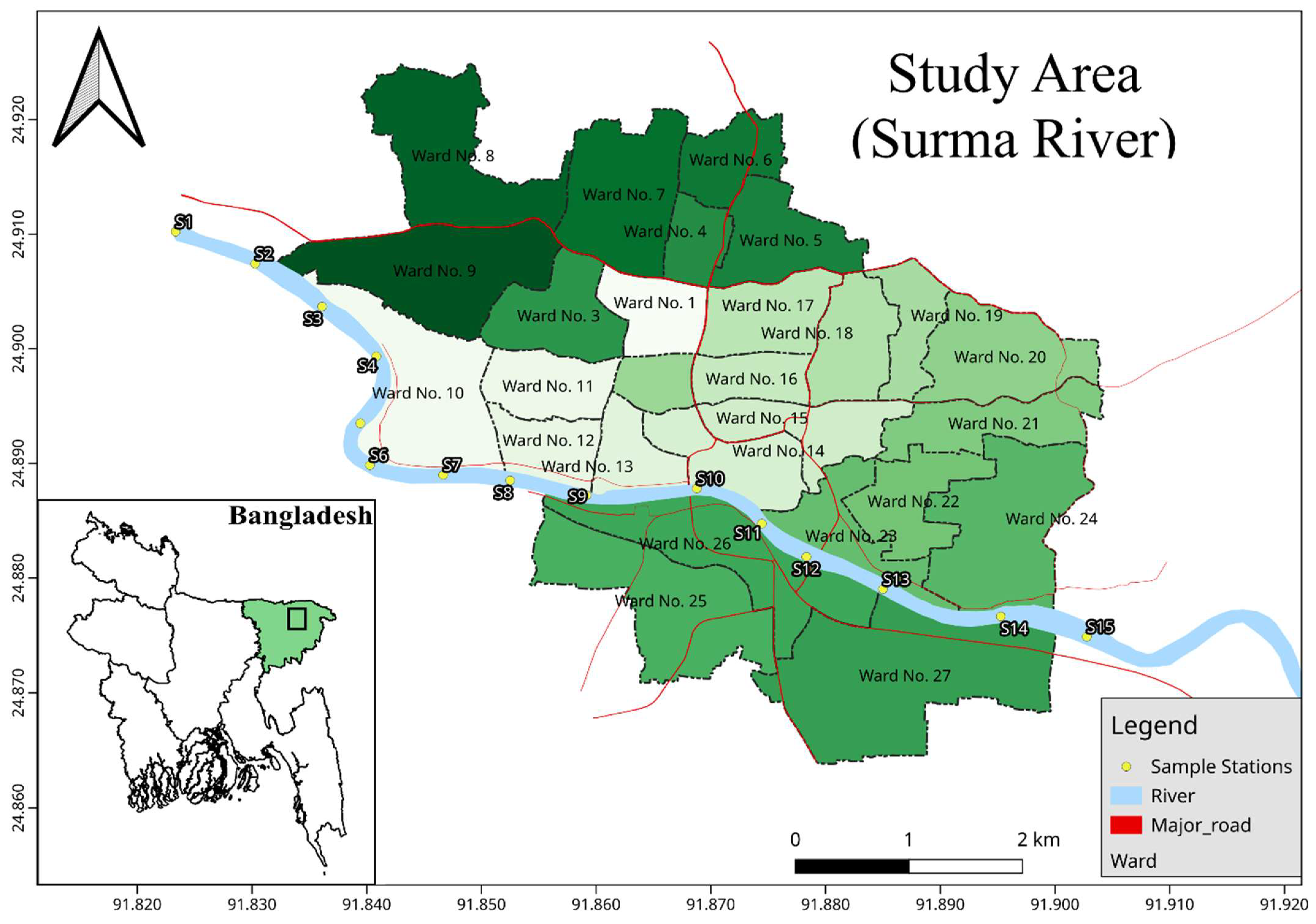
2.1. Study Area

The study was conducted on the Surma River, which forms the longest river system, the Surma–Meghna river system (669 km), in Bangladesh, and flows through the north-eastern city of Sylhet. Sylhet City is located at 24°53′ N latitude and 91°53′ E longitude, with an estimated population of 0.6 million, and a population growth rate of 4% per annum [20], in contrast with the annual growth rate of 2.01% in Bangladesh [22]. The study river originates from the Shillong Hills in Meghalaya, India. Our study river starts from its source, which is the slopes of the Naga–Manipur catchment area, and is known as River Barak. The river gets divided into two distinct branches at Cachar in Assam District in India. The northern branch is known as Surma, which enters Bangladesh through the Sylhet District, and the southern branch is Kushiara. Both of these distributary rivers meet at Madna at the lower segment of the river courses [23]. The river segment covering the metropolitan encroachment limits (from Tukerbazar Ghat to Kushi Ghat) was selected as the study area, owing to the increasing major industrial activity, agricultural activity, and urban land use in this region. The study area is, as shown in Figure 1, located at the Sylhet Metropolitan stretch, which is approximately 15 km within the latitudes 24°54′36.81″ N 24°52′29.64″ N, and longitudes 91°49′23.9988″ E 91°54′10.0008″ E. The geographical coordinates of the sampling locations are given in the Table S1 in the supplementary file. A pilot survey was conducted in the area before sample collection. A total of 15 sampling locations were selected, and are shown in Figure 1.

2.2. Sample Collection and Preparation

Fifteen sediment samples were collected from the selected sampling locations. Sampling locations were selected based on locational interest, such as industrial sewage outlets and municipality sewage outlets. Sediment samples were collected from a depth of 0–30 cm with a 1.5 m long PVC corer (RFL Group, Dhaka, Bangladesh) with 10 cm diameter, manually attached with a galvanized iron pipe (Simex Bangladesh, Dhaka, Bangladesh) and transferred in polyethylene bags immediately. All geographical coordinates were taken with a handheld GPS device (Garmin eTrex 32x, American multinational technology company, Olathe, KS, USA). Before the sampling procedure, the polyethylene bags were cleansed with a diluted 10% nitric acid solution and distilled water [24,25]. Samples were brought to the Soil Resource Development Institute (SRDI), Sylhet, Bangladesh. The sediment samples were air-dried in a dry, dust-free room at room temperature. The samples were grounded after discarding the plant roots and inorganic debris, and sieved with a 2 mm sieve.

2.3. Heavy Metal Analysis

2.3.1. Reagents and Sample Digestion

All standard solutions and reagents, along with acids and chemicals are provided by Merck (Darmstadt, Germany) and MilliporeSigma (Burlington, MA, USA). All used chemical substances were of 99.99% purity level.

Soil Extraction and Determination of Fe, Mn, Cu, and Zn

Soil was weighed 10 g, and taken into a 1.25 mL dry polyethylene bottle. A DTPA (diethylenetriaminepentaacetic acid) solution of 20 mL was added with a pipette. The solution was shaken continuously for exactly 2 h on a horizontal shaker, and filtered immediately after shaking thoroughly by Whatman no. 42 filter paper into a conical flask. The contents of metals in the DTPA extract of soil were determined by AAS (Model Shimadzu AA 7000 series, Shimadzu corporation, Kyoto, Japan) using appropriate cathode lamps. Direct readings of copper and zinc were taken from AAS. For iron (Fe) and manganese (Mn), the reading was taken after the solution was diluted further. The solution was diluted after mixing 5 mL of the solution to 45 mL of distilled water [26].

Soil Extraction and Determination of Ni, Pb, Cd

Sediment sample was weighed 2 g into a 50 mL crucible, to which 10 mL concentrated nitric acid was added. The mixture was kept for 30–45 min for oxidation. After cooling, 2.5 mL of perchloric acid of 70% strength was added, and the mixture was reheated until the digest was clear. Then, the sample was filtered using Whatman no. 42 filter paper. Upon adding distilled water, the mixture was shifted to a volumetric flask, ready to be analyzed by AAS [26].

2.3.2. Analytical Technique and Quality Assurance

All of the soil matrixes were analyzed for Fe, Mn, Cu, Zn, Ni, Pb, and Cd by atomic absorption spectrophotometer (Model Shimadzu AA 7000 series). AAS conditions for analytical measurement are tabulated in Table S2 of the supplementary files. Glassware and all containers used were purified with 20% nitric acid and de-ionized water, and air-dried before usage. The quality of the data obtained from analyzed elements through AAS were thoroughly maintained. The calibration curves were maintained linear for all elements to be studied, after which the performance of the calibrated system was checked. The analytical procedure was checked using a reference soil sample provided by Soil Resource Development Institute, (SRDI, Sylhet, Bangladesh).

3. Results

3.1. Heavy Metal in Sediments

Heavy metal concentrations in river soil determined by AAS are tabulated in Table S3 in supplementary file. The mean concentrations were found as 2.68 mg/kg for Cu; 6.12 mg/kg for Zn; 291.1 mg/kg for Fe; 88.03 mg/kg for Mn, 11.73 mg/kg for Pb; 0.06 mg/kg for Cd; and 92.34 mg/kg for Ni. All metal concentration values are given Table S3 in supplementary section. The results indicate that nearly all of the studied metals failed to exceed the background values given by [27]. This suggests that the investigated area is being enriched with a low quantity of metal content in a massive volume of sediment [28]. The metal concentrations in the study area were found to be in following order: Fe > Mn > Ni > Pb > Zn > Cu > Cd. The total findings of the heavy metal from collected samples are given below in

Table 1. Heavy metal concentration in the bottom sediment of Surma River with descriptive statistics.

Sample Stations	Heavy Metals (Units in mg/kg)
	Cu	Zn	Fe	Mn	Pb	Cd	Ni
Mean	3.688	8.951	317.533	120.136	18.975	0.099	116.077
Standard Deviation	1.867	6.196	70.224	88.473	12.278	0.101	39.248
Minimum	1.590	2.350	170.000	4.200	1.080	0.015	65.560
Maximum	8.520	19.800	418.000	303.490	41.230	0.350	189.620
Surface rock average [27]	32	127	35900	750	16	0.2	49
WHO (2004)	1.5	123	NA	NA	NA	6	20
USEPA (1999)	16	110	30	30	40	0.6	16

. According to this study, the river sediment has low iron concentrations, despite iron being one of the most dominant metals in the earth surface. Such a low iron concentration in the sediment can be attributed to the distinct geochemical setting of the Sylhet region. The bedrock of Sylhet region is dominated mostly with shale, nummulitic limestone, and sandstones, which have fewer Fe-oxides.

A comparative scenario of heavy metal pollution in other major rivers around the world along with the studied river is given below in

Table 2. Comparison of metals in sediment with other studies around the globe (units in mg/kg).

River/Date of Sampling/Country	Pb	Cd	Zn	Ni	Fe	Mn	Cu	Reference
World Average	230.75	1.4	303	102.1	57405.9	975.3	122.9	[23]
Euphrates, 1997, Iraq	19.5	0.08	30	125	-	450	-	[29]
Tigris, 1993, Iraq	17.9–30.6	0.1–1.7	8.3–47.1	105.4–125.5	-	451.3–565.6	17.4–28.9	[30]
Cauvery 2007–2009, India	4.3	1.3	93.1	27.7	11144	176.3	11.2	[31]
Bangshi River, 2014, Bangladesh	59.99	0.61	117.15	25.67	-	483.44	-	[32]
Yangtze, 2005, China	49.19	0.98	230.9	41.86	-	-	60.03	[33]
Surma River, 2019, Bangladesh	11.73	0.06	6.12	92.34	291.1	88.03	2.68	Present study

.

3.2. Assessment of Sediment Quality

Values from background levels (continental shale value or crustal abundance of different elements) can be used as a reference to measure the increase in concentration levels [34]. It is measured in contrast to the values from pre-industrial levels [35]. Due to the unavailability of the background values for this study area, this study utilized the world rock surface values for the assessment of pollution indices [36]. Following pollution, indices were applied to obtain a satisfactory relative ranking of samples: (i) Contamination Factor (CF), (ii) Contamination Degree (CD), (iii) Modified Degree of Contamination (MCD), (iv) Enrichment Factor (EF), (v) Pollution Load Index (PLI), (vi) Geo-Accumulation Index (IGeo).

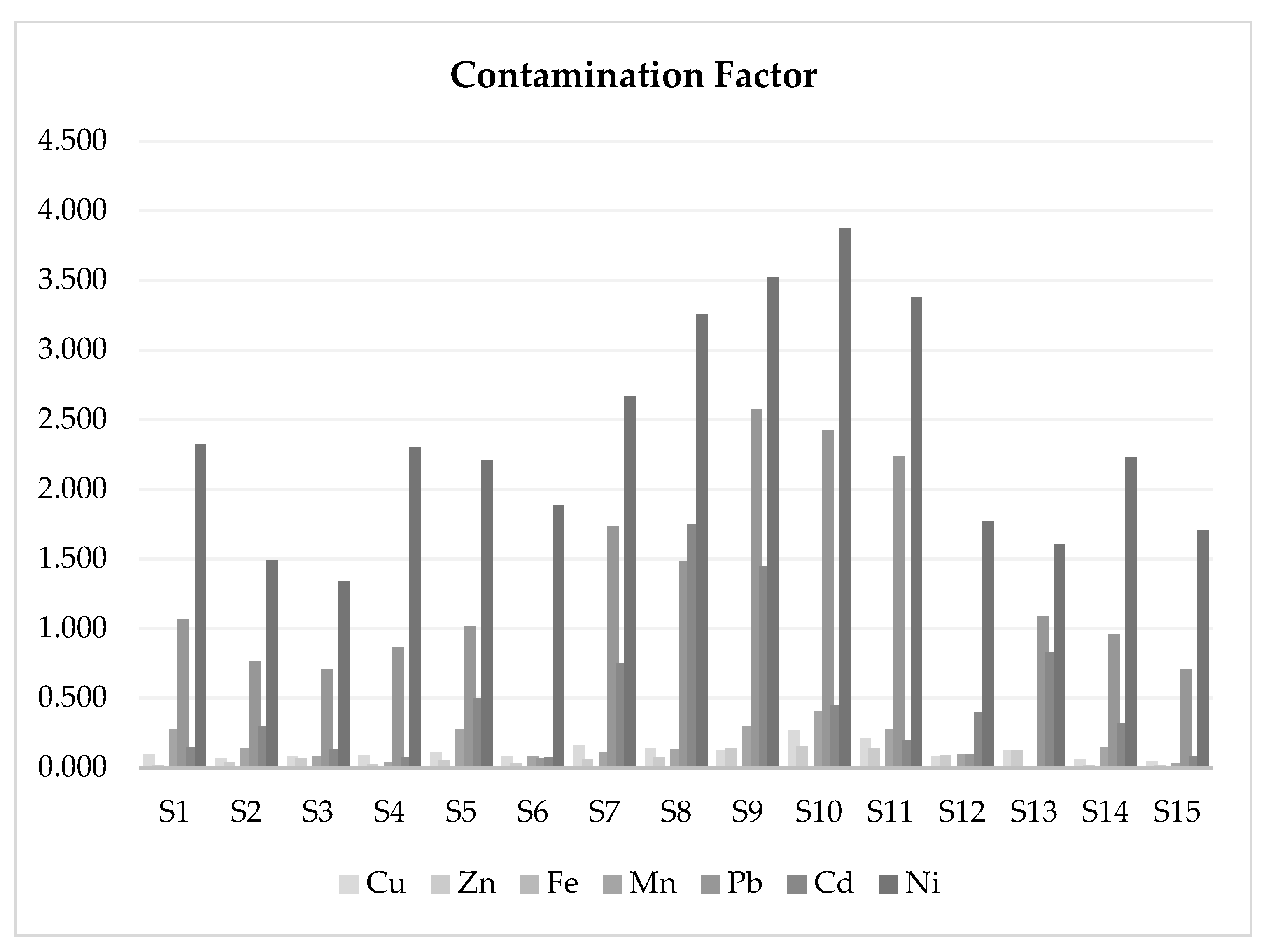
3.2.1. Contamination Factor (CF)

Contamination Factor (CF) and Contamination Degree (CD) together are considered primary indicators of metal pollution status of the subjected soil or sediment [24]. The CF can be obtained for each of the sampling locations by dividing the metal concentrations in sediment by the background concentration values of the respective metals. The CF is the result of dividing the metal concentration in the sediment by the concentration of background value of the respective metal [37]. Ref [38] proposed the following equation to calculate CF and the proposed gradation for CF is tabulated in

Table 3. Description of Contamination Factor (CF) and Contamination Degree (CD) according to [38].

Contamination Factor Ranges	Description	Contamination Degree Ranges	Description
CF < 1	low contamination	CD < 8	Low degree of contamination
1 ≤ CF ≤ 3	Moderate Contamination	8 ≤ CD < 16	Moderate degree of contamination
3 ≤ CF ≤ 6	Considerable Contamination;	16 ≤ CD < 32	Considerable degree of contamination
CF ≥ 6	Very High Contamination	CD ≥ 32	Very high degree of contamination

.

$$\mathrm{CF}=\frac{\mathrm{Cm}\left(\mathrm{sample}\right)}{\mathrm{Cm}\left(\mathrm{Background}\right)}$$

(1)

where Cm _Sample is the metal concentration derived from river sediment, and Cm _Background is the standard metal concentration value equal to the world surface rock average given by [27]. Contamination factors are graded into four classes. Contamination Degree is the summation of all CF values for each sample. Figure 2 contains the CF profile of the study river.

$$\mathrm{CD}={\displaystyle \sum }\left(\mathrm{CF}\right)$$

(2)

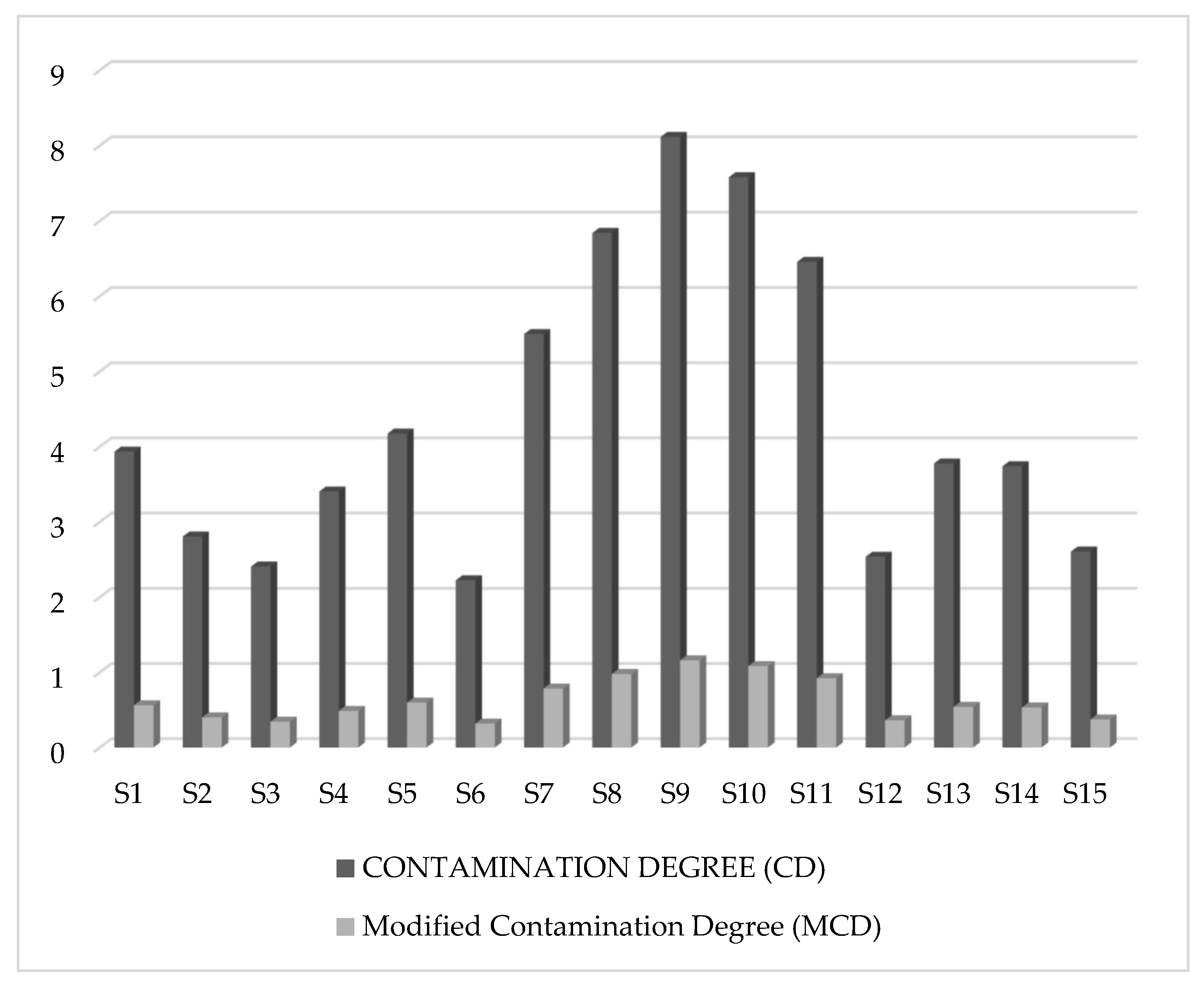
3.2.2. Contamination Degree (CD)

The study area falls into CD range “CD < 8” predominantly, as most of the sampling locations have CD values below 8. However, sample stations S9 and S10 have a moderate degree of contamination, probably due to the sampling locations being situated adjacent to the industrial vicinity.

3.2.3. Modified Contamination Degree, MCD

Ref [39] gave a more simplified method of measuring Contamination Degree, previously given by Hakanson [38]. The formula is given below:

$$\mathrm{M}\mathrm{C}\mathrm{D}=\frac{{\displaystyle \sum }\mathrm{C}\mathrm{F}}{\mathrm{n}}$$

(3)

where n = number of analyzed elements, and CF = Contamination Factor.

In Figure 3, the categories of MCD are shown, which are used to describe and classify the Modified Contamination Degree.

Following are the proposed MCD classes: MCD < 1.5 indicates a significantly low degree of contamination; 1.5 ≤ MCD < 2 designates a low degree of contamination in the sediment; a moderate degree of contamination occurs when MCD levels fall between 2 ≤ MCD < 4; a high degree of contamination is evident in soil when MCD levels rise as high as 4 ≤ MCD < 8; MCD values of an even higher range, 8 ≤ MCD < 16, indicate a very high degree of contamination in the sediment; 16 ≤ MCD < 32 indicates an extremely high degree of contamination in the sediment; and finally, an ultra-high degree of contamination is indicated by MCD levels in the range of ≤32 [39]. In the present study, the MCD values of all sample stations MCD are below 1.5, which indicates a nil-to-very-low degree of contamination. The MCD values are shown in Figure 3.

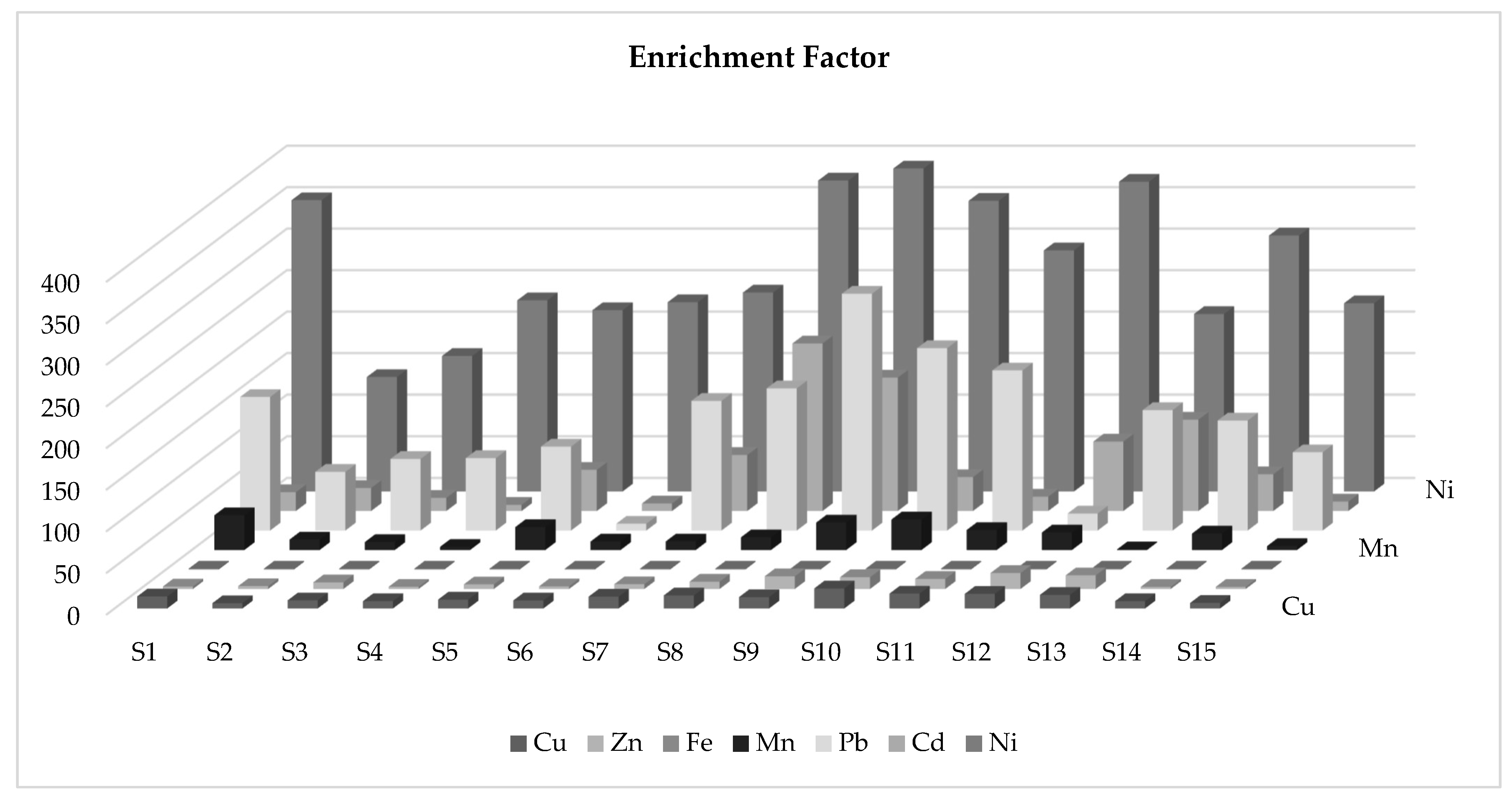
3.2.4. Enrichment Factor (EF)

Ref [40] designated the enrichment factor as an indicator to quantify the anthropogenic contribution to any change in the metal concentration in the sediment. The enrichment factor for the metals can be calculated by the following equation given by [41]:

$$\mathrm{E}\mathrm{F}=\frac{\left(\raisebox{1ex}{$\mathrm{M}\mathrm{e}$}\!\left/ \!\raisebox{-1ex}{$\mathrm{F}\mathrm{e} $}\right.\right) \mathrm{s}\mathrm{a}\mathrm{m}\mathrm{p}\mathrm{l}\mathrm{e}}{\left(\raisebox{1ex}{$\mathrm{M}\mathrm{e}$}\!\left/ \!\raisebox{-1ex}{$\mathrm{F}\mathrm{e} $}\right.\right) \mathrm{b}\mathrm{a}\mathrm{c}\mathrm{k}\mathrm{g}\mathrm{r}\mathrm{o}\mathrm{u}\mathrm{n}\mathrm{d}}$$

(4)

where (Me/Fe) sample is the ratio of subjected metal and Fe of the sediment from sampling location, and, on the other hand, (Me/Fe) background denotes the environmental background value of the metal–Fe ratio. Values of metal concentrations of surface world rocks were chosen as reference, owing to the lack of background values of pre-industrial times [27]. Iron was elected as the suitable element for normalization between the two sets of values from both the metal–Fe ratio of the sample and backgrounds used previously by [36,42]. Enrichment factor is graded in five classes: EF values less than 2 indicate deficiency to minimum enrichment; moderate enrichment is expressed by EF ranging from 2 ≤ EF < 5; values ranging from 5 ≤ EF < 20 indicate significant enrichment; metal enrichment is very high when EF values fall between 20 ≤ EF < 40; and lastly, EF ≥ 40 indicates extremely high enrichment. Heavy metals in River Surma posed following metal enrichment trend shown in Figure 4.

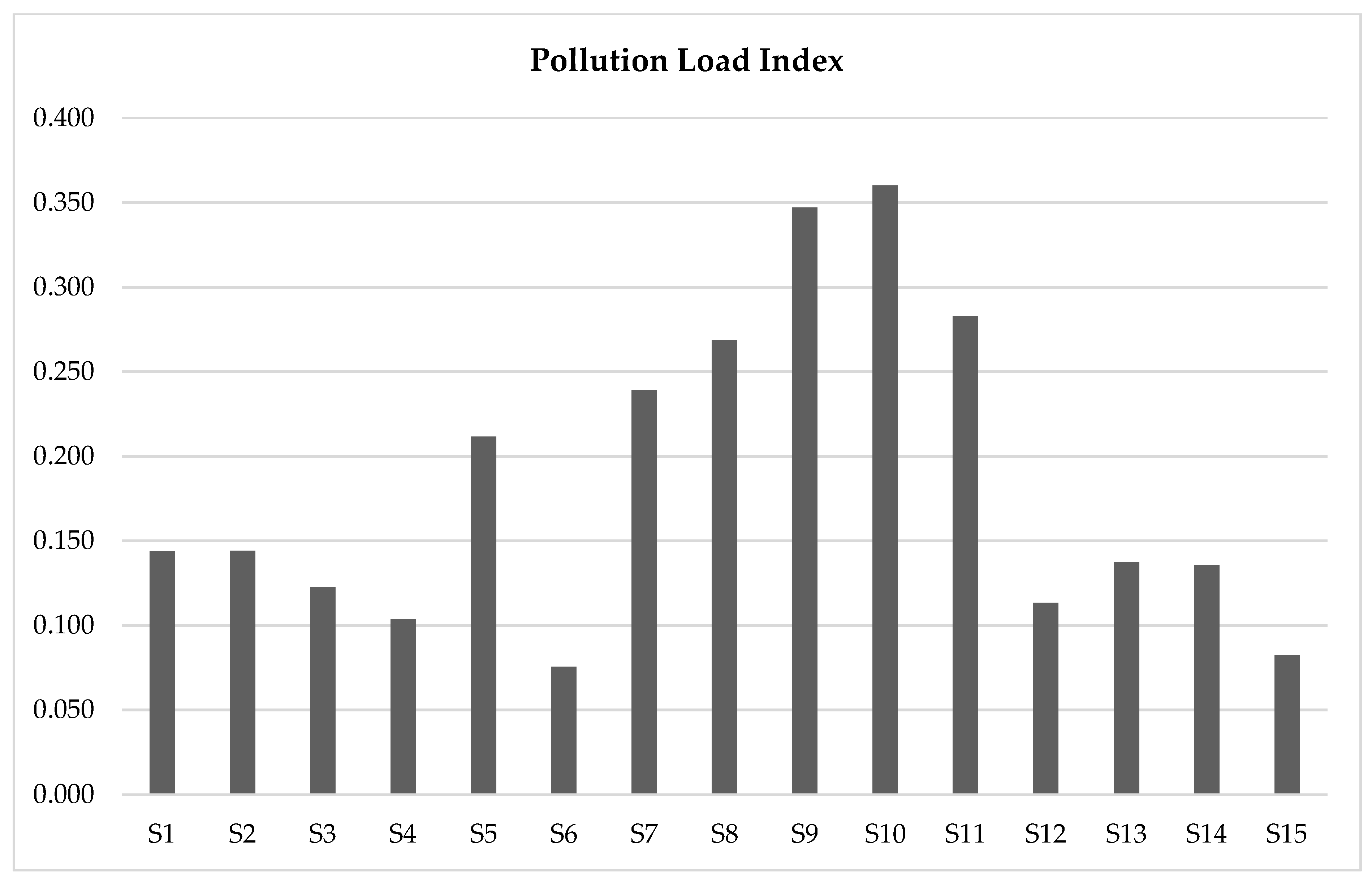
3.2.5. Pollution Load Index (PLI)

Pollution Load Index is a frequently used method for estimating the quality and toxicity of sediment proposed by Tomlinson et al. [43]. The PLI of a particular site is generally estimated by calculating the n^th root of the product of multiplying n-numbered CF values for all investigated elements. The following equation was used for the determination of PLI:

$$\mathrm{P}\mathrm{L}\mathrm{I}={\left(\mathrm{C}\mathrm{F}1\times \mathrm{C}\mathrm{F}2\times \mathrm{C}\mathrm{F}3\times \dots \times \mathrm{C}\mathrm{F}\mathrm{n}\right)}^{\frac{1}{\mathrm{n}}}$$

(5)

where CF denotes the contamination factor, and n is the considered number of metals. There are three discrete categories for pollution measurement with this index. Perfect pollution status is indicative of no pollution when the PLI values are 0 (the first category); the second category is indicative of the baseline degree of pollution when the PLI values are equal or less than 1; and the third category (when PLI is greater than 1) designates progressive decline in terms of pollution of the sites. The PLI values for respective sampling locations are shown in Figure 5.

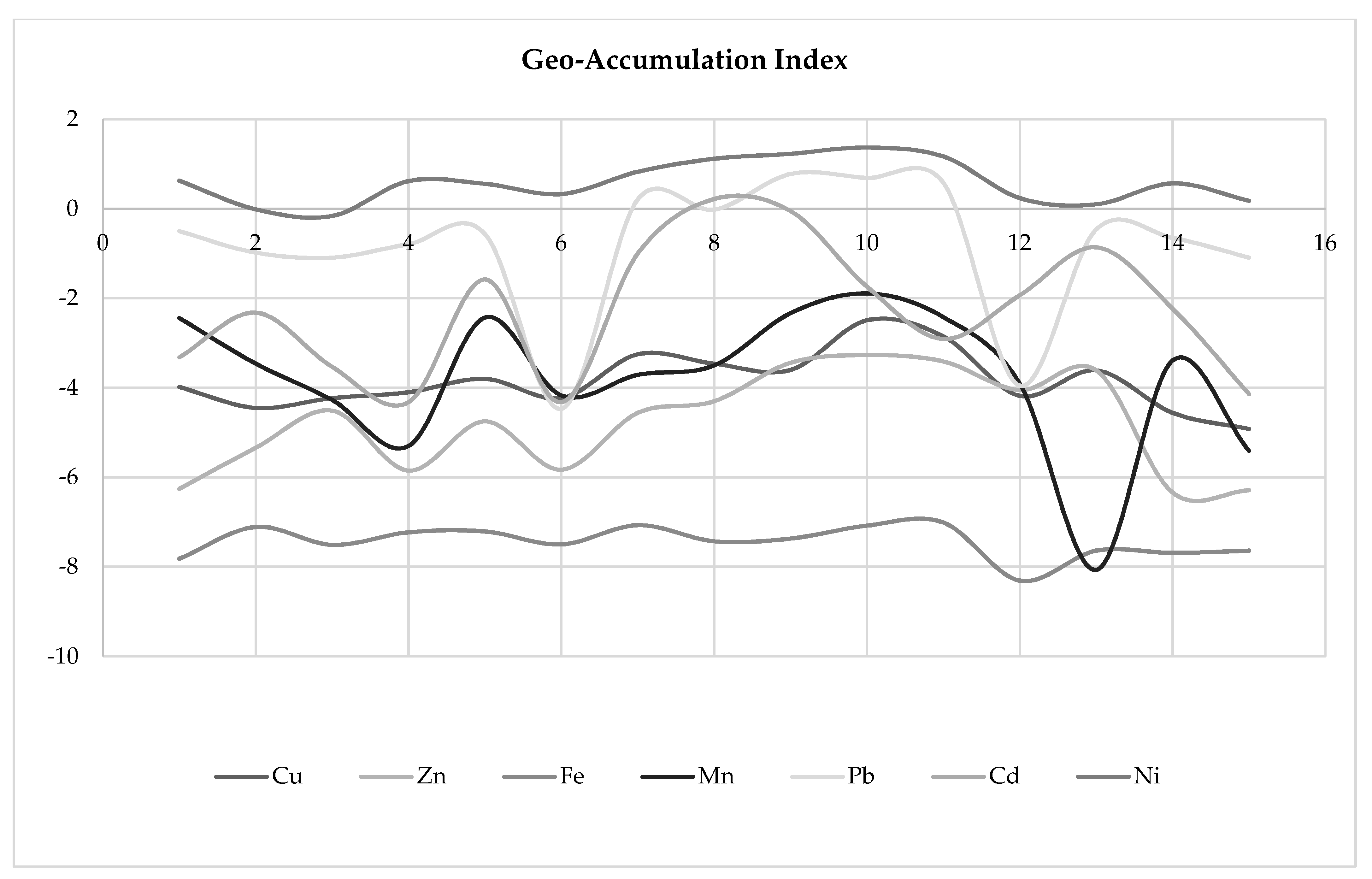
3.2.6. Geo-Accumulation Index (Igeo)

Geo-accumulation index (Igeo) is a method of estimating the enrichment of metal concentration above background values proposed by Muller [44]. The equation used to determine Igeo values is:

$$\mathrm{I}\mathrm{g}\mathrm{e}\mathrm{o}={\log }_2\frac{\mathrm{C}\mathrm{m} \left(\mathrm{S}\mathrm{a}\mathrm{m}\mathrm{p}\mathrm{l}\mathrm{e}\right)}{1.5\times \mathrm{C}\mathrm{m} \left(\mathrm{B}\mathrm{a}\mathrm{c}\mathrm{k}\mathrm{g}\mathrm{r}\mathrm{o}\mathrm{u}\mathrm{n}\mathrm{d}\right)}$$

(6)

where C_m Sample is the concentration of a particular element in the sample, and C_m Background is the geochemical background value of the metal. The values from world rock surface averages given by [27] are used as reference background value [36]. Geo-accumulation index produces results in seven classes of purity. These classes are portrayed in

Table 4. Geo-accumulation Index categories [45,46].

Igeo Class	Igeo Values	Description
Class 0	Igeo < 0	uncontaminated sediments
Class I	0 < Igeo < 1	uncontaminated to moderately contaminated
Class II	1 < Igeo < 2	moderately contaminated
Class III	2 < Igeo < 3	moderately to highly contaminated
Class IV	3 < Igeo < 4	highly contaminated
Class V	4 < Igeo < 5	highly to extremely contaminated
Class VI	Igeo > 5	extremely contaminated

. From the achieved results, it is evident that for most of the sites and metals, the Igeo values remained below 0, depicting uncontaminated sediments, whereas nickel (Ni) and cadmium (Pb) showed some deviance from the trend and fall in class 1. Geo-accumulation Index values of the heavy metals in river sediment are shown in the following Table 4. Figure 6 shows the variability of the Igeo values for the metal concentrations in the sediment.

3.3. Pearson’s Correlation Matrix

Pearson’s Correlation (PC) was calculated for examined metal elements to investigate if there is any correspondence among the elements. Pearson’s Correlation matrix corroborates inter-metal characteristics in terms of origin and behavior along their paths of transport [47]. The results are tabulated below in

Table 5. Pearson’s Correlation Matrix of heavy metals.

	Cu	Zn	Fe	Mn	Pb	Cd	Ni
Cu	1
Zn	0.78 ***	1
Fe	0.58 **	0.29	1
Mn	0.66 ***	0.48 *	0.39	1
Pb	0.78 ***	0.71 ***	0.6 **	0.69 ***	1
Cd	0.26	0.45 *	0.06	0.15	0.49 *	1
Ni	0.8 ***	0.61 **	0.48 *	0.74 ***	0.87 ***	0.5 *	1

* is significant at 0.05 < p ≤ 0.1 levels, ** is significant at 0.01 ≤ p ≤ 0.05 levels, and *** is significant at p < 0.01 levels.

.

Existing metal concentrations in the bottom sediment of river Surma stipulate the concurrent levels of correlation with each other at significant levels of p ≤ 0.05 and p < 0.01 (Table 5). In the present study, Cu, Zn, Ni, and Pb showed significant correlation coefficients, which indicates that they have common sources of origin, and could be dominated by an exclusive factor. Cu displayed soaring levels of a positive relationship with Zn, Mn, and Pb, and in a moderate degree with Fe. The correlation matrix demonstrates that Cu has a low level of relationship with Cd, which points to the possibility of a different origin of these elements. Ni is found to be corresponding and intercorrelated with Cu, Mn, and Pb significantly (at p < 0.01 levels), and moderately with Zn (at 0.01 ≤ p ≤ 0.05 levels), which is associated with common sources of input of heavy metal to the river from municipal waste, agricultural runoff, and industrial sewage. Poor correlations between Fe and Cd could be resulting from the differential sources of origin, where Fe has a natural origin and Cd has anthropogenic origins. Copper and cadmium also deviate from the possibility of being originated from undifferentiated sources, and this difference can be ascribed to the copiousness of Cd in common anthropogenic sources, such as industrial effluents and municipal waste; on the other hand, the original sources of copper can be attributed to agricultural runoffs. Zn, Cu, and Cd also possibly have origins in natural fluvial sediment.

3.4. Potential Ecological Risk Index (PERI)

Refs. [38,48] proposed the PERI method to evaluate the environmental characteristics due to heavy metal contamination in fluvial sediments. Ref. [49] evaluated concurrent pollution levels, and the environmental response to the pollution. The equations employed to determine the ecological risk of a certain area are:

$$\mathrm{R}\mathrm{I}={\displaystyle \sum }({\mathrm{E}}_{{\mathrm{r}}^{\mathrm{i} }})$$

(7)

$${\mathrm{E}}_{{\mathrm{r}}^{\mathrm{i} }}={\mathrm{T}}_{{\mathrm{r}}^{\mathrm{i}}}\times \mathrm{C}\mathrm{F}$$

(8)

Here,

• RI = risk factor or summation of all individual potential ecological risk factors contributed by each meal element;
• E_rⁱ = factor of potential ecological risk;
• CF = contamination factor;
• T_rⁱ = toxic response factor.

According to Hakanson [33], elements such as Ni, Cd, Pb, Zn, and Cu have toxic response factors (T_rⁱ) of 5, 30, 5, 1, and 5, respectively. As per Hakanson’s suggestion [38], E_rⁱ and RI are two terms to be multiplied together for calculating ecological risk. According to this approach, the potential ecological risk is minimal when E_rⁱ < 40; a moderate level of risk for 40 ≤ E_rⁱ ≤ 80; 80 ≤ E_rⁱ ≤ 160 portrays a considerable level of risk; 160 ≤ E_rⁱ ≤ 320 depicts a staggering level of potential ecological risk; whereas E_rⁱ > 320 is construed as a very high ecological risk. Whereas a total ecological risk (RI) value below 150 points indicates a low ecological risk; 150 < RI < 300 suggests moderate degree of ecological risk; a considerable level of ecological risk is generally designated by RI values between 300 to 600; and, ultimately, RI > 600 tends to portray a very high ecological risk of the study area. According to

Table 6. Potential ecological risk and Risk index values.

Site ID	Cu	Zn	Pb	Cd	Ni	RI
S1	0.48	0.02	5.31	4.5	11.62	21.930
S2	0.34	0.04	3.81	9	7.45	20.640
S3	0.4	0.07	3.53	3.9	6.69	14.590
S4	0.44	0.03	4.34	2.25	11.5	18.560
S5	0.54	0.06	5.09	15	11.03	31.720
S6	0.4	0.03	0.34	2.25	9.42	12.440
S7	0.79	0.06	8.67	22.5	13.33	45.350
S8	0.68	0.08	7.42	52.5	16.27	76.950
S9	0.62	0.14	12.88	43.5	17.6	74.740
S10	1.33	0.16	12.12	13.5	19.35	46.460
S11	1.04	0.14	11.19	6	16.89	35.260
S12	0.41	0.09	0.48	11.85	8.83	21.660
S13	0.61	0.12	5.44	24.75	8.03	38.950
S14	0.32	0.02	4.78	9.6	11.16	25.880
S15	0.25	0.02	3.53	2.55	8.51	14.860

, the E_rⁱ values of Pb, Cd, Cu, Ni, Zn in all sampling sites stipulated values predominantly lower than 40, as to specify low levels of ecological risk, except for Cd. Moderate ecological risks are observed for Cd. All of the sample stations can be categorized with low ecological risk levels, as the Risk Index (RI) values are less than 150.

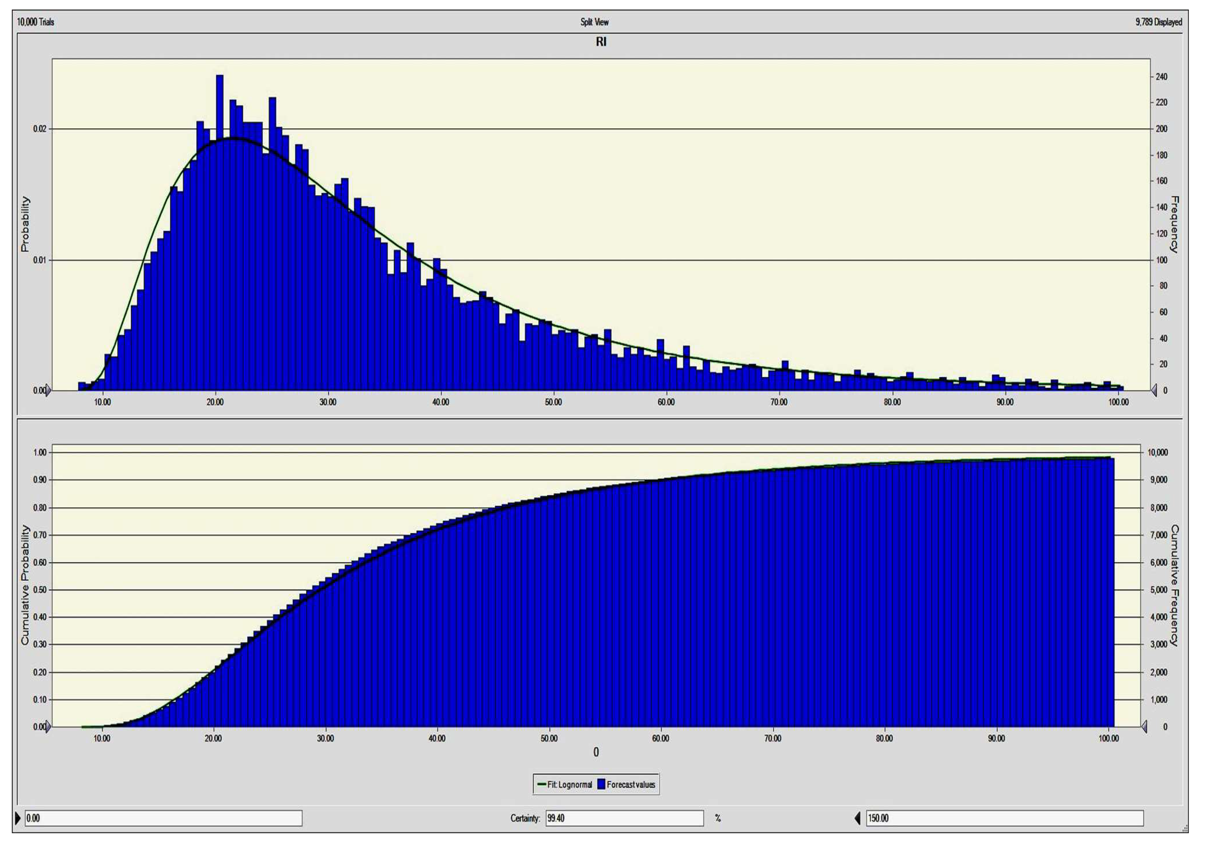
3.5. Monte Carlo Simulation

Generally, Monte Carlo Simulation is performed to elucidate the uncertainty issue, which is intrinsic to the calculation of potential ecological risk using absolute point values of metal concentration. In this method, a suitable dataset is developed, which agrees with a particular probability distribution [50]. The elemental concentrations of the river sediment acted as the primary dataset for finding apposite probability distribution and simulation of RI. According to the Kolmogorov–Smirnov test, the most suitable fitting was demonstrated by the log-normal probability distribution function, whereas other notable density functions with poor fitting included log-logistic, BetaPERT, Weibull, gamma, max-extreme density functions. Ten-thousand Monte Carlo iterations were carried out employing the software CrystalBall (Oracle Corporation, Santa Clara, CA, USA). Repeated calculation produced probability distribution for the Hakanson Risk Index. The output distribution for RI followed a log-normal distribution.

The results from the Monte Carlo Simulation produced probabilistic ecological risk values (E_rⁱ) for heavy metals. Nickel (Ni) indicates a 100% probability to fall under the E_rⁱ value of 40, which indicates low ecological risk shown in Figure S1. Lead (Pb) exhibited a probability of 98.25% to fall in the low-risk category, and 1.51% for moderate potential ecological risk shown in Figure S2. Cadmium (Cd) portrayed a 92.04% probability for the low-risk category, 6.22% in moderate ecological risk, and a 1.49% probability of considerable potential ecological risk shown in Figure S3. Zinc (Zn) and Copper (Cu) both depicted low-risk potential ecological risk probabilities shown in Figure S4 and Figure S5 respectively in supplementary Files. In Figure 7, 100% of the cumulative probability of Risk Index (RI) values is less than 150, which, according to Hakanson’s Risk Index, is representative of low ecological risk. From the sensitivity analysis, it is evident that 67.3% of risk is contributed by Cd, followed by Pb with 2.4%, and Ni with 10.3% variance.

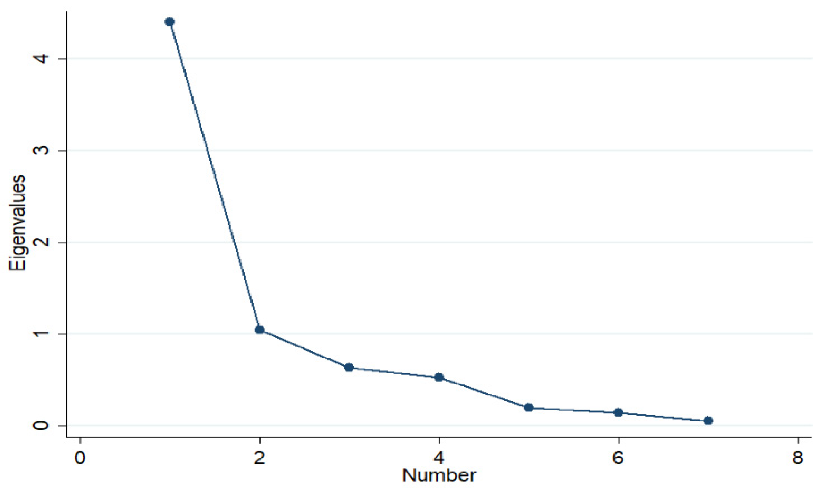
3.6. Principal Component Analysis

PCA was applied to determine the factor responsible for deteriorating the surface water quality. It signifies the association between components and variables. An eigenvalue greater than 1 was considered to define the components. As a result, two principal components were found whose eigenvalues were greater than 1. Figure 8 shows that the scree plot reaches a sharp decline after getting an eigenvalue of 1. PC1 has an eigenvalue of 4.40, and PC2 has 1.04. Moreover, Pb, Ni, and Cu were found to have higher PC1 values, respectively, compared to other parameters. On the other hand, Cd and Fe have lower PC1 values. Besides, PC2 dominated with a higher range of negative values. Fe, Mn, and Cu have negative PC2 values, whereas Cd has a higher positive PC2 value. However, PC1 and PC2 explain 63% and 78% cumulative variance, whereas these two components have 71% and 25% total variance, as per Figure 8. Scree plot of the metals shows Pb > Cu > Ni> Zn > Fe > Cd trend in terms of variance in

Table 7. Principal Component Analysis.

Variables	PC1	PC2
Cu	0.43	−0.16
Zn	0.38	0.23
Fe	0.29	−0.52
Mn	0.37	−0.24
Pb	0.45	0.03
Cd	0.23	0.77
Ni	0.44	0.06
Eigenvalue	4.40	1.04
Cumulative variance (%)	63.00	78.00
Total variance (%)	71.00	25.00

.

Agglomerated hierarchical cluster analysis sorted sampling stations according to their magnitude. It clustered the sampling sites using the dendrogram approach. Four clusters were found to have identical characteristics each. Figure 9 elaborately depicts that S5, S9, S11, and S10 have different features within their cluster. S1, S8, S12, and S14 have comparatively lower values within the cluster. This indicates that the cluster of sampling stations had lower pollution. Cluster analysis implies the degree of pollution over the sampling stations.

4. Discussion and Conclusions

The study demonstrated the concentration of several heavy metals in the river bottom sediment, and systematically examined the ecological risk by employing PERI and Monte Carlo Simulation. However, the result of the present investigation indicates that the comprehensive ecological risk posited by heavy metals in the Surma River does not exceed the lowest limits of Hakanson’s RI index for all heavy metals. This joint approach secures the lessening of the problems of underestimation and overestimation regarding the estimation of ecological risks. Analyses of heavy metal with Hakanson’s RI index and Monte Carlo Simulation in the urban river sediment are very significant for the monitoring and management of river pollution in the developing world, as the urbanized and densely populated cities contribute a huge amount of domestic sewage directly discharged in the river [51]. The river sediment is reported to be marginally contaminated, and probably provides sustenance to the dependent flora and fauna without posing any ecological threat at present. However, grim reports from other similar studies [32,46] from rivers of Bangladesh provide a viewpoint from where River Surma is not far from degrading eventually. The study provides useful tools for future study combined with land use and land cover change, public health issues, and other ecological parameters, which would help decision-makers in the formulation of rules and guidelines about the sustainable management of domestic sewage disposal, and aid in minimizing negative impacts on riverine organisms and the environment. This study suggests that proper focus should be employed on monitoring the point sources of metals entering the river water from nearby cities, and also on the reduction of urban domestic sewage discharge and industrial effluent.

References

1. Silambarasan, K.; Senthilkumar, P.; Velmurugan, K. Studies on the distribution of heavy metal concentrations in River Adyar, Chennai, Tamil Nadu. Eur. J. Exp. Biol. 2012, 2, 2192–2198. [Google Scholar]
2. Barakat, A.; El Baghdadi, M.; Rais, J.; Nadem, S. Assessment of Heavy Metal in Surface Sediments of Day River at Beni-Mellal Region, Morocco. Res. J. Environ. Earth Sci. 2012, 4, 797–806. [Google Scholar]
3. Shazili, N.A.M.; Yunus, K.; Ahmad, A.S.; Abdullah, N.; Rashid, M.K.A. Heavy metal pollution status in the Malaysian aquatic environment. Aquat. Ecosyst. Healh Manag. 2006, 9, 137–145. [Google Scholar] [CrossRef]
4. Islam, M.S.; Ahmed, M.K.; Raknuzzaman, M.; Habibullah-Al-Mamun, M.; Islam, M.K. Heavy metal pollution in surface water and sediment: A preliminary assessment of an urban river in a developing country. Ecol. Indic. 2015, 48, 282–291. [Google Scholar] [CrossRef]
5. Karaca, A.; Cetin, S.C.; Turgay, O.C.; Kizilkaya, R. Effects of Heavy Metals on Soil Enzyme Activities. In Soil Heavy Metals; Sherameti, I., Varma, A., Eds.; Springer: Berlin/Heidelberg, Germany, 2010; pp. 237–262. [Google Scholar]
6. Duruibe, J.; Egwurugwu, J. Heavy metal pollution and human biotoxic effects. Int. J. Phys. Sci. 2007, 2, 112–118. [Google Scholar]
7. Saleem, M.; Iqbal, J.; Shah, M.H. Geochemical speciation, anthropogenic contamination, risk assessment and source identification of selected metals in freshwater sediments—A case study from Mangla Lake, Pakistan. Environ. Nanotechnol. Monit. Manag. 2015, 4, 27–36. [Google Scholar] [CrossRef] [Green Version]
8. Moore, F. Assessment of heavy metal contamination in water and surface sediments of the Maharlu saline lake, SW Iran. Iran. J. Sci. Technol. Trans. A 2009, 33, A1. [Google Scholar]
9. Jaishankar, M.; Tseten, T.; Anbalagan, N.; Mathew, B.B.; Beeregowda, K.N. Toxicity, mechanism and health effects of some heavy metals. Interdiscip. Toxicol. 2014, 7, 60–72. [Google Scholar] [CrossRef] [PubMed] [Green Version]
10. Go’mez-Ariza, J.; Gira’ldez, I.; Sa’nchez-Rodas, D.; Morales, E. Metal readsorption and redistribution during the analytical fractionation of trace elements in toxic estuarine sediments. Anal. Chim. Acta 1999, 399, 295–307. [Google Scholar] [CrossRef]
11. Lasheen, M.; Ammar, N. Speciation of some heavy metals in River Nile sediments, Cairo, Egypt. Environmentalist 2009, 29, 8–16. [Google Scholar] [CrossRef]
12. Qu, C.; Li, B.; Wu, H.; Wang, S.; Li, F. Probabilistic ecological risk assessment of heavy metals in sediments from China’s major aquatic bodies. Stoch. Environ. Res. Risk Assess. 2016, 30, 271–282. [Google Scholar] [CrossRef]
13. Duke, L.D.; Taggart, M. Uncertainty factors in screening ecological risk assessments. Environ. Toxicol. Chem. 2009, 19, 1668–1680. [Google Scholar] [CrossRef]
14. Chen, S.; Fath, B.D.; Chen, B. Information-based network environ analysis: A system perspective for ecological risk assessment. Ecol. Indic. 2011, 11, 1664–1672. [Google Scholar] [CrossRef]
15. Chen, S.; Chen, B.; Fath, B.D. Assessing the cumulative environmental impact of hydropower construction on river systems based on energy network model. Renew. Sustain. Energy Rev. 2015, 42, 78–92. [Google Scholar] [CrossRef]
16. Wang, D. Sustainable management of the future environment under uncertainties and risks. Hum. Ecol. Risk Assess. 2010, 16, 1249–1254. [Google Scholar] [CrossRef]
17. Yu, J.J.; Qin, X.S.; Larsen, O. Joint Monte Carlo and possibilistic simulation for flood damage assessment. Stoch. Environ. Res. Risk Assess. 2013, 27, 725–735. [Google Scholar] [CrossRef]
18. Bai, J.; Cui, B.; Chen, B.; Zhang, K.; Deng, W.; Gao, H.; Xiao, R. Spatial distribution and ecological risk assessment of heavy metals in surface sediments from a typical plateau lake wetland. China Ecol. Model. 2011, 222, 301–306. [Google Scholar] [CrossRef]
19. Su, L.; Liu, J.; Christensen, P. Spatial distribution and ecological risk assessment of metals in sediments of Baiyangdian wetland ecosystem. Ecotoxicology 2011, 20, 1107–1116. [Google Scholar] [CrossRef]
20. Sakib, A.N.; Rahman, A.; Iqbal, S.A.; Das, S.; Yousuf, A. Solid waste management of Sylhet city in terms of energy. In Proceedings of the International Conference on Mechanical Engineering and Renewable Energy 2011, Chittagong, Bangladesh, 22–24 December 2011. [Google Scholar]
21. Larsen, W.E.; Gilley, J.R.; Linden, D.R. Consequences of Waste Disposal on Land. Soil Water Conserv. 1975, 2, 68. [Google Scholar]
22. Ahmed, M.F. Municipal Waste Management in Bangladesh with Emphasis on Recycling, Aspect of Solid Waste Management Bangladesh Context; Mofizul Hoq, L., Ed.; German Cultural Institute: Dhaka, Bangladesh, 1994; p. 113. [Google Scholar]
23. Rashid, H.E. Geography of Bangladesh; The University Press Limited (UPL): Dhaka, Bangladesh, 1977. [Google Scholar]
24. Manoj, K.; Kumar, B.; Padhy, P.K. Characterization of Metals in Water and Sediments of Subarnarekha River along the Projects’ Sites in Lower Basin. Univ. J. Environ. Res. Technol. 2012, 2, 402–410. [Google Scholar]
25. Rabee, A.M.; Al-Fatlawy, Y.F.; Abd, A.A.H.N.; Nameer, M. Using Pollution Load Index (PLI) and Geoaccumulation Index (I-Geo) for the Assessment of Heavy Metals Pollution in Tigris River Sediment in Baghdad Region. J. Al-Nahrain Univ. Sci. 2011, 14, 108–114. [Google Scholar] [CrossRef]
26. Petersen, L. Analytical Methods: Soil, Water, Plant Material, Fertilizer; Soil Resource Development Institute: Dhaka, Bangladesh, 2002. [Google Scholar]
27. Martin, J.M.; Meybeck, M. Elemental mass-balance of material carried by major world rivers. Mar. Chem. 1979, 7, 173–206. [Google Scholar] [CrossRef]
28. Herut, B.; Hornung, H.; Krom, M.D.; Kress, N.; Cohen, Y. Trace metals in shallow sediments from the Mediterranean coastal region of Israel. Mar. Pollut. Bull. 1993, 26, 675–682. [Google Scholar] [CrossRef]
29. Kassim, T.; Al-Saadi, H.; Al-Lami, A.; Al-Jaberi, H. Heavy Metals in Water, Suspended Particles, Sediments and Aquatic Plants of the Upper Region of Euphrates River, Iraq. J. Environ. Sci. Health 1997, 32, 2497–2506. [Google Scholar] [CrossRef]
30. Al-Juboury, A. Natural Pollution by Some Heavy Metals in the Tigris River, Northern Iraq. Int. J. Environ. Res. 2009, 31, 189–198. [Google Scholar]
31. Raju, K.V.; Somashekar, R.; Prakash, K. Heavy Metal Status of Sediment in River Cauvery, Karnataka. Environ. Monit. Assess. 2012, 184, 361–373. [Google Scholar] [CrossRef]
32. Rahman, M.S.; Saha, N.; Molla, A.H.; Al-Reza, S.M. Assessment of Anthropogenic Influence on Heavy Metals Contamination in the Aquatic Ecosystem Components: Water, Sediment, and Fish. Soil Sediment Contam. Int. J. 2014, 23, 353–373. [Google Scholar] [CrossRef]
33. Wang, Y.; Yang, Z.; Shen, Z.; Tang, Z.; Niu, J.; Gao, F. Assessment of Heavy Metals in Sediments from a Typical Catchment of the Yangtze River, China. Environ. Monit. Assess. 2011, 172, 407–417. [Google Scholar] [CrossRef]
34. Christophoridis, C.; Dedepsidis, D.; Fytianos, K. Occurrence and distribution of selected heavy metals in the surface sediments of Thermaikos Gulf, N. Greece. Assessment using pollution indicators. J. Hazard. Mater. 2009, 168, 1082–1091. [Google Scholar] [CrossRef]
35. Turekian, K.K.; Wedepohl, K.H. Distribution of the elements in some major units of the earth’s crust. Geol. Soc. Am. Bull. 1961, 72, 175–192. [Google Scholar] [CrossRef]
36. Salah, E.A.M.; Zaidan, T.A.; Al-Rawi, A.S. Assessment of Heavy Metals Pollution in the Sediments of Euphrates River, Iraq. J. Water Resour. Prot. 2012, 4, 1009–1023. [Google Scholar] [CrossRef] [Green Version]
37. Varol, M. Assessment of heavy metal contamination in sediments of the Tigris River (Turkey) using pollution indices and multivariate statistical techniques. J. Hazard. Mater. 2011, 195, 355–364. [Google Scholar] [CrossRef]
38. Hakanson, L. An ecological risk index for aquatic pollution control. A sedimentological approach. Water Res. 1980, 14, 975–1001. [Google Scholar] [CrossRef]
39. Abrahim, G.M.S.; Parker, R.J. Assessment of heavy metal enrichment factors and the degree of contamination in marine sediments from Tamaki Estuary, Auckland, New Zealand. Environ. Monit. Assess. 2008, 136, 227–238. [Google Scholar] [CrossRef]
40. Feng, H.; Han, X.; Zhang, W.; Yu, L. A preliminary study of heavy metal contamination in Yangtze River intertidal zone due to urbanization. Mar. Pollut. Bull. 2004, 49, 910–915. [Google Scholar] [CrossRef]
41. Sinex, S.A.; Helz, G.R. Regional geochemistry of trace elements in Chesapeake Bay sediments. Environ. Geol. 1981, 3, 315–323. [Google Scholar] [CrossRef]
42. Tippie, V.K. An Environmental Characterization of Chesa-Peak Bay and a Framework for Action. In The Estuary as a Filter; Kennedy, V., Ed.; Academic Press: New York, NY, USA, 1984; pp. 467–487. [Google Scholar]
43. Tomlinson, D.L.; Wilson, J.G.; Harris, C.R.; Jeffrey, D.W. Problems in the assessment of heavy-metal levels in estuaries and the formation of a pollution index. Helgol. Meeresunters. 1980, 33, 566–575. [Google Scholar] [CrossRef] [Green Version]
44. Muller, G. The Heavy Metal Pollution of the Sediments of Neckers and Its tributary, A Stocktaking. Chem. Zeit. 1981, 150, 157–164. [Google Scholar]
45. Bhuiyan, M.A.H.; Parvez, L.; Islam, M.A.; Dampare, S.B.; Suzuki, S. Heavy metal pollution of coal mine-affected agricultural soils in the northern part of Bangladesh. J. Hazard. Mater. 2010, 173, 384–392. [Google Scholar] [CrossRef] [PubMed]
46. Bhuyan, M.S.; Bakar, M.A.; Akhtar, A.; Hossain, M.B.; Ali, M.M.; Islam, M.S. Heavy metal contamination in surface water and sediment of the Meghna River, Bangladesh. Environ. Nanotechnol. Monit. Manag. 2017, 8, 273–279. [Google Scholar] [CrossRef]
47. Suresh, G.; Ramasamy, V.; Meenakshisundaram, V.; Venkatachalapathy, R.; Ponnusamy, V. Influence of mineralogical and heavy metal composition on natural radionuclide concentrations in the river sediments. Appl. Radiat. Isot. 2011, 69, 1466–1474. [Google Scholar] [CrossRef] [PubMed]
48. Hakanson, L. Metal monitoring in coastal environments. Met. Coast. Environ. Lat. Am. 1988, 239–257. [Google Scholar] [CrossRef]
49. Devanesan, E.; Gandhi, M.S.; Selvapandiyan, M.; Senthilkumar, G.; Ravisankar, R. Heavy metal and Potential Ecological Risk Assessment in sedimentscollected from Poombuhar to Karaikal Coast of Tamilnadu using Energy dispersive X-ray fluorescence (EDXRF) technique. Beni-Suef Univ. J. Basic Appl. Sci. 2017, 6, 285–292. [Google Scholar] [CrossRef]
50. Li, X.; Chi, W.; Tian, H.; Zhang, Y.; Zhu, Z. Probabilistic ecological risk assessment of heavy metals in western Laizhou Bay, Shandong Province, China. PLoS ONE 2019, 14, e0213011. [Google Scholar] [CrossRef] [PubMed] [Green Version]
51. Withanachchi, S.S.; Ghambashidze, G.; Kunchulia, I.; Urushadze, T.; Ploeger, A. Water Quality in Surface Water: A Preliminary Assessment of Heavy Metal Contamination of the Mashavera River, Georgia. Int. J. Environ. Res. Public Health 2018, 15, 621. [Google Scholar] [CrossRef] [Green Version]
Figure 1. Study area and sampling stations.
Water 14 00180 g001
Figure 2. Contamination Factor of heavy metals at all sample stations.
Water 14 00180 g002
Figure 3. CD and MCD values of the heavy metals of the river sediment.
Water 14 00180 g003
Figure 4. Metal enrichment of all heavy metals in River Surma.
Water 14 00180 g004
Figure 5. Pollution Load Index values of sampling sites at Surma River.
Water 14 00180 g005
Figure 6. Igeo variation in the sediment of River Surma.
Water 14 00180 g006
Figure 7. Probability and cumulative probability of Risk Index (RI) Value.
Water 14 00180 g007
Figure 8. Scree plot of PCA.
Water 14 00180 g008
Figure 9. Cluster analysis.
Water 14 00180 g009