
Effects of Barrier Stiffness on Debris Flow Dynamic Impact—II: Numerical Simulation


1
Department of Geotechnical Engineering, College of Civil Engineering, Tongji University, Shanghai 200092, China
2
Key Laboratory of Geotechnical and Underground Engineering of the Ministry of Education, Tongji University, Shanghai 200092, China
*
Author to whom correspondence should be addressed.
Water 2022, 14(2), 182; https://doi.org/10.3390/w14020182
Submission received: 23 November 2021
/
Revised: 30 December 2021
/
Accepted: 5 January 2022
/
Published: 10 January 2022
(This article belongs to the Special Issue Mechanism and Prevention of Debris Flow Disaster)
Abstract
:The destructive and impactful forces of debris flow commonly causes local damage to engineering structures. The effect of a deformable barrier on the impact dynamics is important in engineering design. In this study, a flow–structure coupled with Smoothed Particle Hydrodynamics model was presented to investigate the effects of barrier stiffness on the debris impact. A comparison of the results of physical tests and simulation results revealed that the proposed smoothed particle hydrodynamics model effectively reproduces the flow kinematics and time history of the impact force. Even slight deflections of the deformable barrier lead to obvious attenuation of the peak impact pressure. Additionally, deformable barriers with lower stiffness tend to deform more downstream upon loading, shifting the deposited sand toward the active failure mode and generating less static earth pressure. When the debris flow has a higher frontal velocity, the impact force on the barrier is dominated by the dynamic component and there is an appreciable effect of the stiffness of the deformable barrier on load attenuation.
1. Introduction
Flow-like landslides are differentiated from landslides by the pervasive, fluid-like deformation of the mobilized material [1], which can travel long distances at high speed (>5 m/s) [2]. It is difficult to classify flow-like landslides which are highly concentrated mixtures of water and solid material. Examples of flow-like landslides are rock avalanches, debris flow, sensitive clay flowslides and mud flows and so on [2]. Flow-like landslides can cause catastrophic losses of human life and property without warning, on account of having destructive impact forces [1,3,4]. The impact disaster caused by flow-like landslides is very serious all over the world [5,6,7,8,9]. As an example, Oso landslide occurred in Snohomish Country, Washington, USA on 22 March 2014, with a flow distance of over 2 km [7], resulting in 43 deaths and an additional economic loss of $120 million [10]. On 20 August 2014, 2 major debris flows occurred in Hiroshima city, southern Japan, resulting in 44 deaths, 74 injuries and the destruction of more than 400 residential buildings [11]. Especially in China, mountainous and hilly areas account for approximately 65% of land resource areas. Hence, the geological conditions are even more serious. In August 2010, a catastrophic debris flow in Zhouqu, China, pulled down almost 5500 houses [12]. Meanwhile, a flow-like landslide with a maximum speed of 74.6 m/s and flow distance of 2.5 km occurred in Maoxian, China, in June 2017, instantly destroying the village of Xinmo at the foot of a slope, demolishing 64 houses, and killing 10 people [13]. Prevention and control measures for flow-like landslides can be divided into: active measures and passive ones [14]. Active measures, such as disaster assessment, early warning system and land planning, etc., lack consideration of disaster mechanisms and are insufficient to reduce risk. Passive measures are engineering structures which are made of concrete, such as barriers, deflecting/catching dams, nets, and baffle piles [15,16,17,18,19,20,21,22,23], have been widely implemented. However, these protective countermeasures are commonly destroyed by geo-flows, causing even greater disaster, because large dynamic impact forces are the main damaging factor as shown by the statistical analysis of failure types for debris flows [24]. An investigation of the dynamic impact of flow–structure interactions is thus important in the design of hazard mitigation structures. The accompanying paper [25] described in detail laboratory flume tests of the debris flow impact on a deformable barrier with varying stiffness. In this paper, an advanced numerical method is introduced for the simulation of the interaction between debris flow and a deformable barrier. The paper provides guidelines for engineers to assess comprehensively the interaction between debris flow and a deformable barrier in similar cases.
Scaling problem is an unavoidable key consideration [26,27] when modelling debris flow in the laboratory test. As an alternative to physical modelling, numerical modelling is a promising method that has commonly been implemented to investigate the impact dynamics of debris flow and to assist in industrial design because of its wide applicability. The simulation of the impact dynamics of debris flows usually involves modeling the large deformation of materials. The finite-element method (FEM) has frequently been applied to solve the large-scale engineering problems mentioned above. Ma et al. [28] used CFX software to analyze the velocity field of debris flow and the size and distribution law of impact force on structure, which played an important role in the optimization design of engineering projects. Li et al. [29] analyzed the bearing capacity of the retaining dam under the impact of debris flow on the ANSYS Workbench platform, and proposed a new type of steel-concrete combined protective structure. However, it is difficult to simulate such large deformation problems of debris flows using the FEM because of severe mesh distortion, inaccurate solutions, and convergence failure [30,31]. Even if the above problems can be solved by remeshing, the modeling remains problematic owing to the time required and the complex nature of the constitutive models [32]. Alternatively, the discrete element method (DEM) can easily handle large deformations owing to its Lagrangian characteristics. Ng et al. [33] analyzed the impact effect of dry debris flow on structures by DEM method, and discussed the influence of different structural forms on flow-structure interaction. However, the DEM remains limited to small-scale problems on account of its computational demand. Additionally, the determination of DEM input parameters remains controversial [34]. In the last few years, a few mesh-free continuum-scale methods of modeling a series of large movements of materials have been developed; e.g., the moving-particle semi-implicit method [35], element-free Galerkin method [36], and finite point method [37]. Among these, the smoothed particle hydrodynamics (SPH) method is robust and reliable in the simulation of debris flows [24,38,39,40,41,42]; the SPH method was initially developed for astrophysical analysis by Gingold and Monaghan [43]. The meshless and Lagrangian nature of the SPH method allows granular-flow materials to be discretized as a series of particles, conveying all of the field variables (e.g., density, position, velocity, and pressure), whose behavior can be obtained directly by solving the Navier–Stokes equations without adopting depth integration or the shallow-water assumption [44]. Sun et al. [45] used SPH method to study the interaction between rock avalanches and protective structure, and put forward reasonable suggestions for optimal design of protective structure based on numerical results. Moreover, Moriguchi et al. [1], Dai et al. [24], Sheikh et al. [46], and He et al. [34] applied the SPH method to simulate the flow behavior of granular materials on rigid structures and obtained promising results. The SPH method is thus adopted in the present work to investigate the effects of the structural stiffness of a deformable barrier on characteristics of the granular flow impact.
This paper establishes an effective fluid–structure coupled SPH model by solving the governing equations of the flow and structure as a regularized Bingham model [47] and an elastic constitutive model, respectively. The results of the flume tests presented in Part I [25] of the study are then used as benchmarks to validate the SPH model. The SPH model is used to further explore the effect of the barrier stiffness on static pressure and the effects of the debris flow frontal velocity on the impact force and response of the deformable barrier.
2. Flow–Structure Coupled SPH Model
2.1. Smooth Function
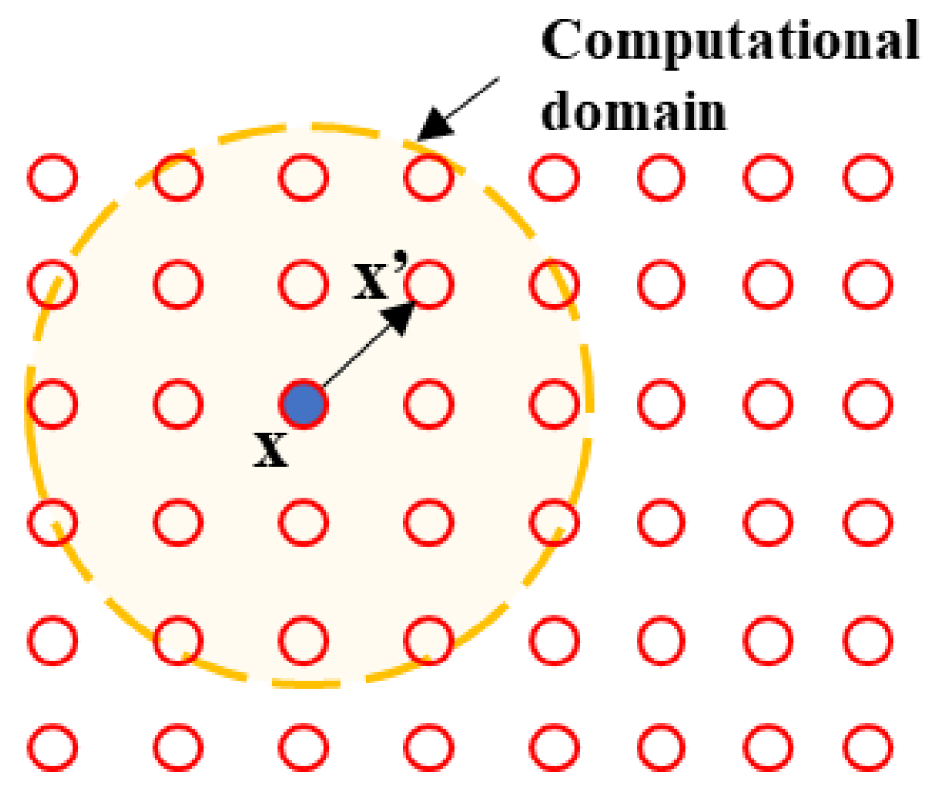
As a continuum-scale mesh-free method, the SPH method discretizes the computational domain using a series of discrete particles conveying all of the field variables. The specific steps of the SPH method are a kernel approximation and particle approximation. The field function f(xi) and its derivative at the position xi can be rewritten as:
where the subscripts i and j, respectively, denote the particle of concern and the neighboring particle in the domain of influence, N is the number of particles within the influence domain of particle i, and are, respectively, the mass and density of the i-th particle, and is the smoothing Kernel function. This work implements the Wendland kernel function, ensuring robust and stable solutions with a relatively high calculation efficiency [48]:
where in 2-dimensional space and is the normalized distance (Figure 1).
To overcome tensile instability when the support domains are incomplete at the boundary, a simple correction was presented by Bonet and Lok [49] to replace the original kernel gradient. The corrected kernel gradient method used in SPH simulation has been shown to exactly reproduce the gradient of a linear function [24].
2.2. Governing Equations
The basic governing (Navier–Stokes) equations of debris flow include the continuity equation and momentum conservation equations, which are written in the Lagrangian framework as:
where ρ and v are, respectively, the bulk density and velocity vector and is the acceleration due to gravity. The Cauchy stress tensor σ is comprises the pressure P and deviatoric stress tensor τ:
The pressure term P is updated using an equation of state, with the elastic pressure being proportional to the change in density:
where ρ0 is a reference density that is commonly taken as the initial density of flow and csound is the speed of sound treated as a numerical constant. We determine that to ensure the ability to describe a solid mechanism referring to previous studies [24], where K is the bulk modulus.
Previous studies demonstrated that the mechanical behaviors of flowing fine sand can be described using rheological models [24,38,42,50,51]. Among these models, the Bingham model is widely used in simulating lava flow, snow avalanches, rock avalanches, and other such granular flows [1,38,52,53,54]. Nevertheless, the Bingham model may be singular when . Here, is the second invariant of the strain rate tensor and is expressed as . In this paper, we adopt the regularized model proposed by Zhu et al. [47]:
where ηapp is the apparent viscosity. is the local strain rate tensor and is expressed as
In the regularized Bingham model, the apparent dynamic viscosity ηapp is expressed as
where the regularization parameter m is used to handle the numerical divergence problem of the equivalent viscosity coefficient under small deformation. In this work, m = 100 is adopted following Li et al. [38]. With this regularization, the apparent dynamic viscosity limit converges to when tends to zero. τy is the Mohr–Coulomb yield stress used to describe the cohesive and frictional behavior of flowing sand and is expressed as
where c is the cohesion of the soil material, φ is the internal frictional angle, and P is the pressure.
The governing equation of the mass of the structure in the Lagrangian frame is written as
where ρ and ρ0 are, respectively, the current and initial densities and J and J0 are respectively the current and initial determinants of the deformation gradient F. We have
where X is the referent coordinate and u = x − X is the current coordinate.
The governing equation of momentum is
where is the interaction force density exerted on the structure by the debris flow. The stress tensor σ is expressed by
where S is the deviatoric stress tensor of structure. The stress–strain relationship is expressed according to Jaumann’s formulation of Hooke’s law as
where μ is the shear modulus of the modeled material, ε is the strain rate tensor, and ω is the rotation rate tensor.
2.3. Setup of the Numerical Model and Simulation Plan
Figure 2 shows that the setup of the numerical model corresponds to the flume model reported in Part I of the study used in this calibration. The sliding surface is inclined at a fixed angle of 45° and has dimensions (length × width × height) of 4000 mm × 400 mm × 1500 mm. A hopper stores sliding sand behind an automatic gate. A barrier with a height of 300 mm is set at a distance of 0.2 m from the foot of the slope. The flume and barrier are, respectively, modeled as rigid and elastic walls as the SPH model is calibrated. The bulk density of the test sand is 1400 kg/m3. The cohesion and friction angle of the sand are, respectively, c = 0 Pa and φ = 34° in the test. The different barrier materials, namely low-density polyethylene, high-density polyethylene, and polypropylene, are, respectively, simulated with elastic moduli of 0.6, 0.8, and 1.0 GPa. Additionally, tests are conducted and the results analyzed to reveal fundamental insights into the impact dynamics of the sand flow for the three cases of barrier stiffness. In addition to ensuring computational efficiency, the test sand and flume are discretized with an initial distance of △r = 0.01 m [24,55]. The key simulation parameters are summarized in Table 1. The hydrodynamic equation F = αρv2hL [56] shows that a change in flow velocity affects the impact force, which might result in a different load attenuation for a deformable barrier with different stiffness. To explore the effects of the frontal velocity of the debris flow, we design a systematical program for the parametric study, which is a function of barrier stiffness and flow velocity (changed by different initial position) as presented in Table 2. Among them, the initial conditions of P_15/S_6, P_15/S_8 and P_15/S_10 were corresponding to that of the experiments conducted in part I [25] (S_6, S_8 and S_10, respectively).
3. Validation of the Flow–Structure Coupled SPH Model
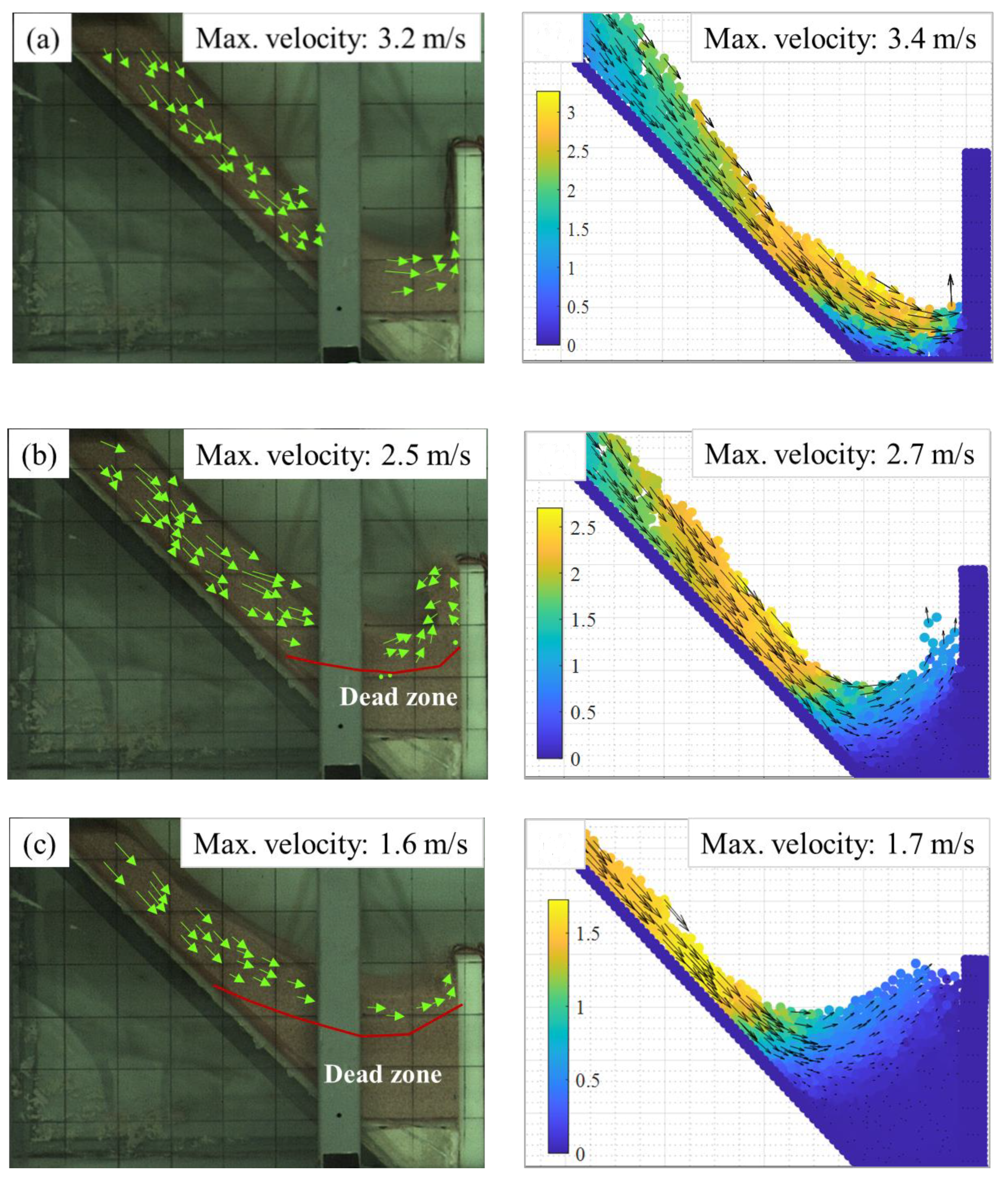
To verify the accuracy and effectiveness of the proposed SPH model, the flow kinematics and impact dynamics simulated using the SPH model are compared with the results of the experiments reported in Part I [25]. Time, t, began as the granular flow struck the barrier in all of the results without specific illustration. Figure 3 compares the velocity fields of the flow obtained through particle image velocimetry (PIV) (left) and flow kinematics computed using the proposed SPH method (right) at several instances for test P_15/S_10. At time t = 0.0 s, a wedge-like flow approached the barrier with a simulated maximum frontal velocity of approximately 3.4 m/s, which is slightly higher than the maximum frontal velocity observed in the test (3.2 m/s). At time t = 0.11 s, the flow struck the barrier with the maximum velocity reduced by about 20% to 2.7 m/s, gradually creating a dead zone near the wall and gradually increasing the loading of the barrier until reaching a peak value. Subsequent flow overtopped the dead zone, providing a cushioning layer, and then began to run up along the surface of the barrier, falling back upon reaching the top. At t = 0.50 s, the maximum flow velocity was 1.7 m/s, the size of the dead zone increased and there was piling up near the barrier as a static equilibrium was reached progressively. There was a small difference of 5% in the maximum velocity between the simulation and the PIV and little difference in the final deposition profiles, showing that the presented SPH model suitably describes the flow kinematics of the flow–structure interaction.
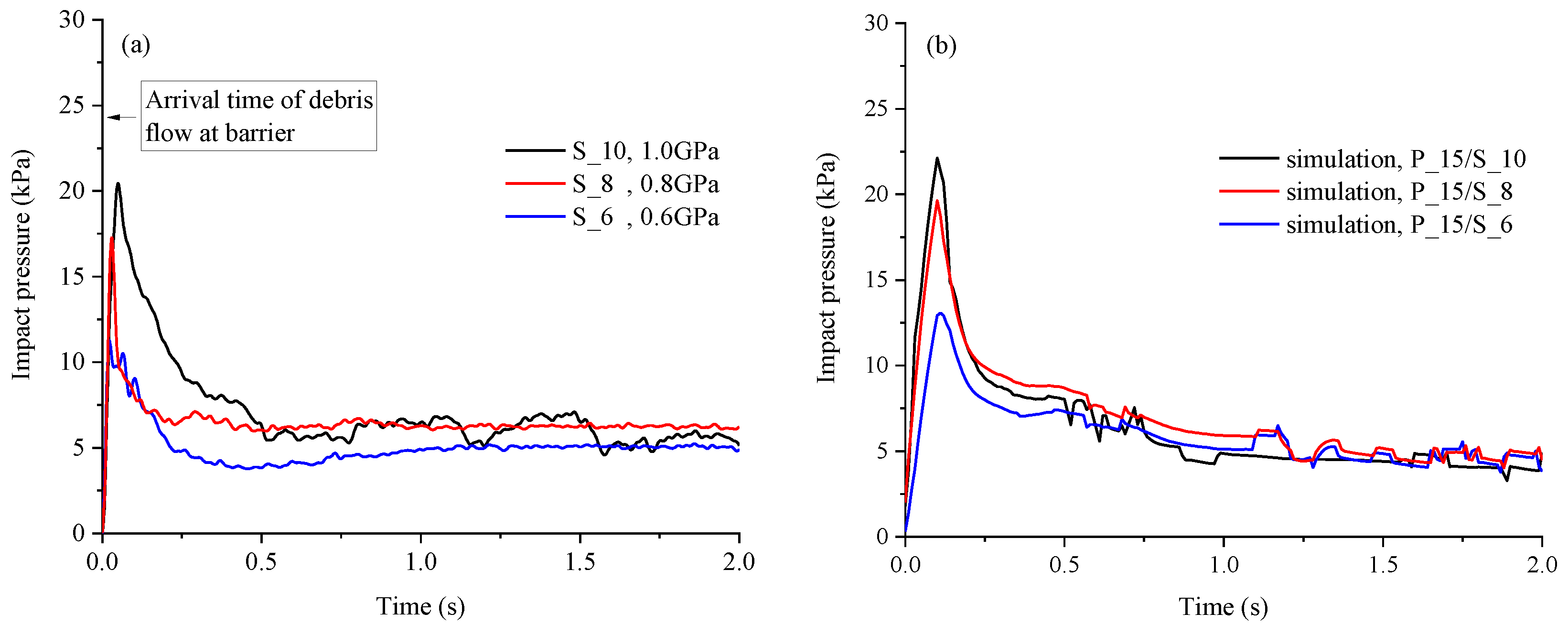
Besides comparing the flow kinematics, the impact dynamics need to be validated for the SPH model. Figure 4a,b show the evolution of the impact forces in the physical flume experiment and numerical simulation for three values of barrier stiffness. The peak impact forces obtained for the barrier were 11.7, 17.3, and 20.4 kPa in the physical experiment and 13.1, 19.5, and 22.1 kPa in simulation for E = 0.6, 0.8, and 1.0 GPa, respectively; i.e., the numerical impact forces were 12%, 12%, and 8% higher than the measurements in the physical experiment. No difference between the physical and numerical impact forces was greater than 12%, demonstrating the alignment between the results of the physical experiment and numerical simulation. The general trends of the change in the strain acting on the barrier at different values of stiffness were well simulated using the proposed SPH method. Additionally, the proposed SPH numerical framework allows for the accurate estimation of the dynamic impact process for the flow–structure interaction if used with an appropriate constitutive model.
4. Interpretation of the Computed Results
4.1. Effects of the Barrier Stiffness on the Earth Pressure Coefficient
Figure 4 shows that the peak impact force attenuated with a decrease in the stiffness of the barrier. Not only did the deflection at peak load attenuate but there was also an effect on the static lateral earth pressure. Figure 5 compares the static earth pressure behind barriers of different stiffness for the final deposition of the sand flow. The mobilization of full passive resistance requires a wall movement on the order of 10–15% of the embedded depth in the case of loose sand; the corresponding mobilization of active pressure is on the order of 1%. Adopting Rankine theory, we calculate the active and passive earth pressure coefficients as Ka = 0.21 and Kp = 4.60, respectively.
As barriers tend to deform in a downstream direction upon loading, the pressure coefficient of the granular material is expected to be close to the active pressure coefficient (Ka). For test P_15/S_10, the back-calculated earth pressure coefficient is 4.19, which is close to the passive pressure coefficient, implying a slight deflection downstream upon loading and the sand flow not being fully mobilized to an active mode. The deduced earth pressure coefficients of tests P_15/S_8 and P_15/S_6 were 2.82 and 1.64, respectively. The deflection of the barrier downstream upon loading increased with decreasing barrier stiffness. The sand flow deposited near the wall moved further with the deformation of the barrier, which in turn incrementally increased the shear energy dissipation of sand layers and shifted the deposited sand toward an active failure mode. These results show that a lower static earth pressure acts on a barrier of lower stiffness, with the earth pressure coefficient being strongly affected by the stiffness of the barrier. Additionally, the distribution of the lateral earth pressure did not reach the passive failure mode for any barrier, implying that the adoption of the passive pressure coefficient (Kp) is suitable for engineering design.
4.2. Effects of the Frontal Velocity
The hydrodynamic equation F = αρv2hL shows that a change in flow velocity affects the impact force, which might result in a different load attenuation for a deformable barrier. To explore the effects of the frontal velocity of the debris flow, the initial position of sand was varied as 1.3, 1.4, 1.6, and 1.7 m in further simulation using the presented fluid–structure coupled SPH model. The peak force and the static force, normalized by the peak force of P_15/S_10, are shown in Table 3. In Table 4, the frontal velocity ζ denotes the normalized frontal velocity which was normalized by the velocity of sand flow having an initial position of 1.5 m (3.4 m/s). The peak impact force, which is normalized by the force for ζ = 1.0, generally increases with the frontal velocity of the debris flow, as expected. And an increase in ζ also results in higher load attenuation. The debris flow with lower frontal velocity carried limited momentum and thus generated a limited peak impact force with low peak-static force ratio on the deformable barrier. At this moment, the deflection may mostly be the result of the static pressure rather than that of the peak impact force [57], inducing slighter deflection of barrier. Correspondingly, when the debris flow has a higher frontal velocity, the impact force on the barrier is dominated by the dynamic component. This generates a greater peak impact force and results in a greater downstream deflection of the deformable barrier with appreciable load attenuation.
However, a natural debris flow is a mixture of water, sand, and boulders and thus has more complex dynamic characteristics. The results of this study relate only to fine sand flow or viscous debris flow and more experimental and simulation results are needed to quantify the effects of the material properties of a debris flow on the load attenuation of the deformable barrier. Meanwhile, there are limitations to the proposed SPH model, and proper constitutive models, which require the capturing of the characteristics of both unsteady flows and dynamic impacts, are needed for better modeling.
5. Discussion
This paper addresses some of the fundamental aspects of debris flow impact barriers with different stiffnesses and the results of the presented SPH model had been compared with the experiments in part I [25]. Generally, good agreements are obtained. However, there are some issues needed to be solved which call for further investigation. For simulations in Section 3, the flows run about 0.2 m/s faster than the experimental measured velocity in our simulation. We found that the Bingham model with Mohr-Coulomb yield criterion is insufficient in debris flow modelling. This discrepancy was also observed in other numerical simulation, showing that an applicable constitutive relation which can describe the multi-stage dynamic behavior of granular flows is requisite for accurate simulation [58]. Flow-like landslides in the natural state present mixtures of water, air and solid grains with different size [2]. In the process of large deformation and high-speed movement, the particles are randomly distributed in space and time, and different flow states coexist, showing unsteady flow characteristics, which leads to the non-stationary impact effect [59,60]. An appropriate constitutive model is needed to provide a more accurate simulation of the dynamic impact process for flow-structure interaction. On the other hand, a hydromechanical coupled SPH model should be developed in future studies for different cases considering the bed entrainment during the propagation of debris flows and the multiphase fluid model. Moreover, numerous experimental results of interaction between debris flow and deformable structures are needed to further validate the presented method so that it can be used more widely in the future.
6. Conclusions
The investigation of the dynamic impact behavior of flow–structure interactions is important to the design of hazard mitigation structures. This work quantitatively analyzed the effects of the barrier stiffness on the impact dynamics using a flow–structure coupled SPH numerical model. The main findings of the study are as follows.
- (1)
- The presented flow–structure coupled SPH modeling solves the governing equations of the flow and structure and considers the flow–structure interaction. A comparison of the results of numerical and physical tests showed that the proposed numerical model can be used to simulate the problem of a large deformation flow effectively and predict the flow kinematics and impact force appropriately;
- (2)
- The deduced static earth pressure coefficients revealed that barriers with lower stiffness tend to deform downstream upon loading, shifting the pressure coefficient of the deposited sand toward the active pressure coefficient (Ka);
- (3)
- The peak impact force generally increases with the frontal velocity of the debris flow. Moreover, the stiffness of the deformable barrier affects the load attenuation when the debris flow has larger frontal velocity, in the situation that the impact force on the barrier is dominated by the dynamic component.
Author Contributions
Conceptualization, Y.H.; methodology, X.J. and J.J.; validation, X.J. and J.J.; formal analysis, X.J. and J.J.; investigation, X.J. and J.J.; data curation, X.J. and J.J.; writing—original draft preparation, X.J.; writing—review and editing, X.J.; visualization, X.J.; supervision, Y.H.; project administration, Y.H.; funding acquisition, Y.H. All authors have read and agreed to the published version of the manuscript.
Funding
This work was supported by the National Natural Science Foundation of China (grant No. 41831291).
Institutional Review Board Statement
Not applicable.
Informed Consent Statement
Not applicable.
Acknowledgments
The authors thank the editor and the reviewers for their help to improve the quality of our manuscript.
Conflicts of Interest
The authors declare no conflict of interest.
References
- Moriguchi, S.; Borja, R.I.; Yashima, A.; Sawada, K. Estimating the impact force generated by granular flow on a rigid obstruction. Acta Geotech. 2009, 4, 57–71. [Google Scholar] [CrossRef]
- Hungr, O.; Leroueil, S.; Picarelli, L. The Varnes classification of landslide types, an update. Landslides 2014, 11, 167–194. [Google Scholar] [CrossRef]
- Choi, S.-K.; Park, J.-Y.; Lee, D.-H.; Lee, S.-R.; Kim, Y.-T.; Kwon, T.-H. Assessment of barrier location effect on debris flow based on smoothed particle hydrodynamics (SPH) simulation on 3D terrains. Landslides 2021, 18, 217–234. [Google Scholar] [CrossRef]
- Marchetti, E.; Walter, F.; Barfucci, G.; Genco, R.; Wenner, M.; Ripepe, M.; McArdell, B.; Price, C. Infrasound Array Analysis of Debris Flow Activity and Implication for Early Warning. J. Geophys. Res.-Earth Surf. 2019, 124, 567–587. [Google Scholar] [CrossRef] [Green Version]
- Allstadt, K. Extracting source characteristics and dynamics of the August 2010 Mount Meager landslide from broadband seismograms. J. Geophys. Res.-Earth Surf. 2013, 118, 1472–1490. [Google Scholar] [CrossRef]
- Guerriero, L.; Revellino, P.; Diodato, N.; Grelle, G.; De Vito, A.; Guadagno, F.M. Morphological and Climatic Aspects of the Initiation of the San Mango Sul Calore Debris Avalanche in Southern Italy. In Engineering Geology for Society and Territory, Proceedings of the 12th International IAEG Congress, Torino, Italy, 15–19 September 2014; Springer: Cham, Switzerland, 2015; Volume 2. [Google Scholar]
- Iverson, R.M.; George, D.L.; Allstadt, K.; Reid, M.E.; Collins, B.D.; Vallance, J.W.; Schilling, S.P.; Godt, J.W.; Cannon, C.M.; Magirl, C.S.; et al. Landslide mobility and hazards: Implications of the 2014 Oso disaster. Earth Planet. Sci. Lett. 2015, 412, 197–208. [Google Scholar] [CrossRef] [Green Version]
- Petley, D. Global patterns of loss of life from landslides. Geology 2012, 40, 927–930. [Google Scholar] [CrossRef]
- Zhang, J.; Gurung, D.R.; Liu, R.; Murthy, M.S.R.; Su, F. Abe Barek landslide and landslide susceptibility assessment in Badakhshan Province, Afghanistan. Landslides 2015, 12, 597–609. [Google Scholar] [CrossRef]
- Wartman, J.; Montgomery, D.R.; Anderson, S.A.; Keaton, J.R.; Benoit, J.; dela Chapelle, J.; Gilbert, R. The 22 March 2014 Oso landslide, Washington, USA. Geomorphology 2016, 253, 275–288. [Google Scholar] [CrossRef]
- Wang, F.; Wu, Y.-H.; Yang, H.; Tanida, Y.; Kamei, A. Preliminary investigation of the 20 August 2014 debris flows triggered by a severe rainstorm in Hiroshima City, Japan. Geoenviron. Disasters 2015, 2, 1. [Google Scholar] [CrossRef] [Green Version]
- Tang, C.; van Asch, T.W.J.; Chang, M.; Chen, G.Q.; Zhao, X.H.; Huang, X.C. Catastrophic debris flows on 13 August 2010 in the Qingping area, southwestern China: The combined effects of a strong earthquake and subsequent rainstorms. Geomorphology 2012, 139, 559–576. [Google Scholar] [CrossRef]
- Xu, Q.; Li, W.; Dong, X.; Xiao, X.; Fan, X.; Pei, X. The Xinmocun landslide on 24 June 2017 in Maoxian, Sichuan: Characteristics and failure mechanism. Chin. J. Rock Mech. Eng. 2017, 36, 2612–2628. [Google Scholar]
- Huebl, J.; Fiebiger, G. Debris-flow mitigation measures. In Debris-Flow Hazards and Related Phenomena; Springer: Berlin/Heidelberg, Germany, 2005. [Google Scholar]
- Albaba, A.; Lambert, S.; Faug, T. Dry granular avalanche impact force on a rigid wall: Analytic shock solution versus discrete element simulations. Phys. Rev. E 2018, 97, 052903. [Google Scholar] [CrossRef] [PubMed]
- Armanini, A.; Rossi, G.; Larcher, M. Dynamic impact of a water and sediments surge against a rigid wall. J. Hydraul. Res. 2020, 58, 314–325. [Google Scholar] [CrossRef] [Green Version]
- Bi, Y.-z.; He, S.-m.; Li, X.-p.; Wu, Y.; Xu, Q.; Ouyang, C.-j.; Su, L.-J.; Wang, H. Geo-engineered buffer capacity of two-layered absorbing system under the impact of rock avalanches based on Discrete Element Method. J. Mt. Sci. 2016, 13, 917–929. [Google Scholar] [CrossRef]
- Chen, H.-X.; Li, J.; Feng, S.-J.; Gao, H.-Y.; Zhang, D.-M. Simulation of interactions between debris flow and check dams on three-dimensional terrain. Eng. Geol. 2019, 251, 48–62. [Google Scholar] [CrossRef]
- Jiang, Y.J.; Fan, X.-Y.; Li, T.-H.; Xiao, S.-Y. Influence of particle-size segregation on the impact of dry granular flow. Powder Technol. 2018, 340, 39–51. [Google Scholar] [CrossRef]
- Ng, C.W.W.; Choi, C.E.; Liu, L.H.D.; Wang, Y.; Song, D.; Yang, N. Influence of particle size on the mechanism of dry granular run-up on a rigid barrier. Geotech. Lett. 2017, 7, 79–89. [Google Scholar] [CrossRef]
- Remaitre, A.; van Asch, T.W.J.; Malet, J.P.; Maquaire, O. Influence of check dams on debris-flow run-out intensity. Nat. Hazards Earth Syst. Sci. 2008, 8, 1403–1416. [Google Scholar] [CrossRef]
- Shen, W.; Wang, D.; Qu, H.; Li, T. The effect of check dams on the dynamic and bed entrainment processes of debris flows. Landslides 2019, 16, 2201–2217. [Google Scholar] [CrossRef]
- Zhou, G.G.D.; Song, D.; Choi, C.E.; Pasuto, A.; Sun, Q.C.; Dai, D.F. Surge impact behavior of granular flows: Effects of water content. Landslides 2018, 15, 695–709. [Google Scholar] [CrossRef]
- Dai, Z.; Huang, Y.; Cheng, H.; Xu, Q. SPH model for fluid-structure interaction and its application to debris flow impact estimation. Landslides 2017, 14, 917–928. [Google Scholar] [CrossRef]
- Huang, Y.; Jin, Y.X.; Ji, J.J. Effects of barrier stiffness on debris flow dynamic impact—I: Laboratory flume test. Water 2021, 3, 26. [Google Scholar]
- Khan-Mozahedy, A.B.M.; Munoz-Perez, J.J.; Neves, M.G.; Sancho, F.; Cavique, R. Mechanics of the scouring and sinking of submerged structures in a mobile bed: A physical model study. Coast. Eng. 2016, 110, 50–63. [Google Scholar] [CrossRef]
- Chen, J.; Chen, X.; Zhao, W.; You, Y. Debris Flow Drainage Channel with Energy Dissipation Structures: Experimental Study and Engineering Application. J. Hydraul. Eng. 2018, 144, 06018012. [Google Scholar] [CrossRef]
- Ma, Z.Y.; Zhang, J.; Liao, H.J. Numerical simulation of viscous debris flow block engineering. Rock Soil Mech. 2007, 28, 389–392. [Google Scholar]
- Li, J.; Wang, X.; Ran, Y. Analysis on bearing performance of new-style steel-concrete combined dam under action of debris flow slurry. Chin. J. Geol. Hazard Control. 2016, 27, 85–94. [Google Scholar]
- Abdelrazek, A.M.; Kimura, I.; Shimizu, Y. Simulation of three-dimensional rapid free-surface granular flow past different types of obstructions using the SPH method. J. Glaciol. 2016, 62, 335–347. [Google Scholar] [CrossRef] [Green Version]
- Chen, W.; Qiu, T. Numerical Simulations for Large Deformation of Granular Materials Using Smoothed Particle Hydrodynamics Method. Int. J. Geomech. 2012, 12, 127–135. [Google Scholar] [CrossRef]
- Bui, H.H.; Fukagawa, R.; Sako, K.; Ohno, S. Lagrangian meshfree particles method (SPH) for large deformation and failure flows of geomaterial using elastic-plastic soil constitutive model. Int. J. Numer. Anal. Methods Geomech. 2008, 32, 1537–1570. [Google Scholar] [CrossRef]
- Ng, C.W.W.; Choi, C.E.; Goodwin, G.R.; Cheung, W.W. Interaction between dry granular flow and deflectors. Landslides 2017, 14, 1375–1387. [Google Scholar] [CrossRef]
- He, X.; Liang, D.; Wu, W.; Cai, G.; Zhao, C.; Wang, S. Study of the interaction between dry granular flows and rigid barriers with an SPH model. Int. J. Numer. Anal. Methods Geomech. 2018, 42, 1217–1234. [Google Scholar] [CrossRef]
- Nohara, S.; Suenaga, H.; Nakamura, K. Large deformation simulations of geomaterials using moving particle semi-implicit method. J. Rock Mech. Geotech. Eng. 2018, 10, 1122–1132. [Google Scholar] [CrossRef]
- Wang, C.; Deng, A.; Taheri, A.; Ge, L. A Mesh-Free Approach for Multiscale Modeling in Continuum-Granular Systems. Int. J. Comput. Methods 2020, 17, 2050006. [Google Scholar] [CrossRef]
- Qin, X.; Hu, G.; Peng, G. Finite Point Method of Nonlinear Convection Diffusion Equation. Filomat 2020, 34, 1517–1533. [Google Scholar] [CrossRef]
- Li, S.; Peng, C.; Wu, W.; Wang, S.; Chen, X.; Chen, J.; Zhou, G.G.D.; Chitneedi, B.K. Role of baffle shape on debris flow impact in step-pool channel: An SPH study. Landslides 2020, 17, 2099–2111. [Google Scholar] [CrossRef]
- Huang, Y.; Zhang, W.; Xu, Q.; Xie, P.; Hao, L. Run-out analysis of flow-like landslides triggered by the Ms 8.0 2008 Wenchuan earthquake using smoothed particle hydrodynamics. Landslides 2012, 9, 275–283. [Google Scholar] [CrossRef]
- Monaghan, J.J.; Kos, A.; Issa, N. Fluid motion generated by impact. J. Waterw. Port Coast. Ocean. Eng. 2003, 129, 250–259. [Google Scholar] [CrossRef]
- Pastor, M.; Yague, A.; Stickle, M.M.; Manzanal, D.; Mira, P. A two-phase SPH model for debris flow propagation. Int. J. Numer. Anal. Methods Geomech. 2018, 42, 418–448. [Google Scholar] [CrossRef]
- Wang, W.; Chen, G.; Han, Z.; Zhou, S.; Zhang, H.; Jing, P. 3D numerical simulation of debris-flow motion using SPH method incorporating non-Newtonian fluid behavior. Nat. Hazards 2016, 81, 1981–1998. [Google Scholar] [CrossRef]
- Gingold, R.A.; Monaghan, J.J. Smoothed Particle Hydrodynamics—Theory and Application to Non-spherical Stars. Mon. Not. R. Astron. Soc. 1977, 181, 375–389. [Google Scholar] [CrossRef]
- Han, Z.; Su, B.; Li, Y.; Dou, J.; Wang, W.; Zhao, L. Modeling the progressive entrainment of bed sediment by viscous debris flows using the three-dimensional SC-HBP-SPH method. Water Res. 2020, 182, 116031. [Google Scholar] [CrossRef] [PubMed]
- Sun, X.P.; He, S.M.; Fan, X.Y.; Tian, S.J.; Zhang, L.L.; Tian, W.G. The effect of particle size on the impact of rockfall debris on obstacles. J. Zhejiang Univ. Technol. 2016, 44, 222–225. [Google Scholar]
- Sheikh, B.; Qiu, T.; Ahmadipur, A. Comparison of SPH boundary approaches in simulating frictional soil-structure interaction. Acta Geotech. 2021, 16, 2389–2408. [Google Scholar] [CrossRef]
- Zhu, H.; Kim, Y.; De Kee, D. Non-Newtonian fluids with a yield stress. J. Non-Newton. Fluid Mech. 2005, 129, 177–181. [Google Scholar] [CrossRef]
- Monaghan, J.J. SPH without a tensile instability. J. Comput. Phys. 2000, 159, 290–311. [Google Scholar] [CrossRef]
- Bonet, J.; Lok, T.S.L. Variational and momentum preservation aspects of Smooth Particle Hydrodynamic formulations. Comput. Methods Appl. Mech. Eng. 1999, 180, 97–115. [Google Scholar] [CrossRef]
- Pastor, M.; Blanc, T.; Haddad, B.; Petrone, S.; Sanchez Morles, M.; Drempetic, V.; Issler, D.; Crosta, G.B.; Cascini, L.; Sorbino, G.; et al. Application of a SPH depth-integrated model to landslide run-out analysis. Landslides 2014, 11, 793–812. [Google Scholar] [CrossRef] [Green Version]
- McDougall, S.; Hungr, O. Dynamic modelling of entrainment in rapid landslides. Can. Geotech. J. 2005, 42, 1437–1448. [Google Scholar] [CrossRef]
- Dragoni, M.; Bonafede, M.; Boschi, E. Downslope flow models of a bingham liquid—Implications for lava flows. J. Volcanol. Geotherm. Res. 1986, 30, 305–325. [Google Scholar] [CrossRef]
- Kaitna, R.; Rickenmann, D.; Schatzmann, M. Experimental study on rheologic behaviour of debris flow material. Acta Geotech. 2007, 2, 71–85. [Google Scholar] [CrossRef]
- Dai, Z.; Huang, Y.; Cheng, H.; Xu, Q. 3D numerical modeling using smoothed particle hydrodynamics of flow-like landslide propagation triggered by the 2008 Wenchuan earthquake. Eng. Geol. 2014, 180, 21–33. [Google Scholar] [CrossRef]
- Bao, Y.; Huang, Y.; Liu, G.R.; Zeng, W. SPH Simulation of High-Volume Rapid Landslides Triggered by Earthquakes Based on a Unified Constitutive Model. Part II: Solid-Liquid-Like Phase Transition and Flow-Like Landslides. Int. J. Comput. Methods 2020, 17, 1850149. [Google Scholar] [CrossRef]
- Hübl, J.; Holzinger, G. Entwicklung von Grundlagen zur Dimensionierung Kronenoffener Bauwerke für die Geschiebebewirtschaftung in Wildbächen: Klassifikation von Wildbachsperren; WLS Report 50; Im Auftrag des BMLFUW VC 7a (Unveröffentlicht); Institut für Alpine Naturgefahren, Universität für Bodenkultur: Wien, Austria, 2003. [Google Scholar]
- Song, D.; Zhou, G.G.D.; Xu, M.; Choi, C.E.; Li, S.; Zheng, Y. Quantitative analysis of debris-flow flexible barrier capacity from momentum and energy perspectives. Eng. Geol. 2019, 251, 81–92. [Google Scholar] [CrossRef]
- Zhan, L.; Peng, C.; Zhang, B.; Wu, W. Three-dimensional modeling of granular flow impact on rigid and deformable structures. Comput. Geotech. 2019, 112, 257–271. [Google Scholar] [CrossRef]
- Huang, Y.; Zhang, B. Challenges and perspectives in designing engineering structures against debris-flow disaster. Eur. J. Environ. Civ. Eng. 2020, 8, 4126. [Google Scholar] [CrossRef]
- Sun, Q.; Jin, F.; Wang, G. The multiscale structure of dense granular matter. Mech. Eng. 2010, 32, 10–15. [Google Scholar]
Figure 1.
Interaction between particles.

Figure 2.
Sketch of the simulated flume model.

Figure 3.
Comparison of impact kinematics at different times (test ID: P_15/S_10): (a) t = 0.00 s, (b) t = 0.11 s, (c) t = 0.50 s; the velocity field of flows through PIV (left); computed flow kinematics through SPH (right).
Figure 3.
Comparison of impact kinematics at different times (test ID: P_15/S_10): (a) t = 0.00 s, (b) t = 0.11 s, (c) t = 0.50 s; the velocity field of flows through PIV (left); computed flow kinematics through SPH (right).

Figure 4.
Histories of the tested (a) and simulated (b) impact forces for different values of barrier stiffness.
Figure 4.
Histories of the tested (a) and simulated (b) impact forces for different values of barrier stiffness.

Figure 5.
Static earth pressure distribution of deposited sand.


Table 1.
Key input parameters of simulation.
| Material Property | Parameters | |
|---|---|---|
| Bulk density | ρ (kg/m) | 1400 |
| Cohesion | c (kPa) | 0.0 |
| Internal friction angle | φ (°) | 34 |
| Equivalent viscosity | η (Pa·s) | 1.0 |
| Young’s modulus of sand | E (GPa) | 0.01 |
| Poisson’s ratio of sand | ν (\) | 0.25 |
| Poisson’s ratio of barrier | ν (\) | 0.30 |
| The initial distance | △r (m) | 0.01 |
| Unit time step | dt (s) | 2.0 × 10⁻⁶ |
Table 2.
Numerical simulation program.
| Test ID | Young’s Modulus/E | Initial Height of Sand |
|---|---|---|
| P_13/S_6 | 0.6 GPa | 1.3 m |
| P_14/S_6 | 1.4 m | |
| P_15/S_6 | 1.5 m | |
| P_16/S_6 | 1.6 m | |
| P_17/S_6 | 1.7 m | |
| P_13/S_8 | 0.8 GPa | 1.3 m |
| P_14/S_8 | 1.4 m | |
| P_15/S_8 | 1.5 m | |
| P_16/S_8 | 1.6 m | |
| P_17/S_8 | 1.7 m | |
| P_13/S_10 | 1.0 GPa | 1.3 m |
| P_14/S_10 | 1.4 m | |
| P_15/S_10 | 1.5 m | |
| P_16/S_10 | 1.6 m | |
| P_17/S_10 | 1.7 m |
Table 3.
The peak force and the static force normalized by the peak force of P_15/S_10.
| Test ID | The Peak Force | The Static Force |
|---|---|---|
| P_13/S_6 | 0.61 | 0.38 |
| P_13/S_8 | 0.71 | 0.46 |
| P_13/S_10 | 0.87 | 0.52 |
| P_14/S_6 | 0.67 | 0.36 |
| P_14/S_8 | 0.78 | 0.45 |
| P_14/S_10 | 0.95 | 0.53 |
| P_15/S_6 | 0.70 | 0.36 |
| P_15/S_8 | 0.82 | 0.47 |
| P_15/S_10 | 1 | 0.51 |
| P_16/S_6 | 0.84 | 0.38 |
| P_16/S_8 | 0.98 | 0.51 |
| P_16/S_10 | 1.18 | 0.54 |
| P_17/S_6 | 0.90 | 0.35 |
| P_17/S_8 | 1.04 | 0.40 |
| P_17/S_10 | 1.25 | 0.45 |
Table 4.
Effects of the frontal velocity on the peak impact forces (F/Fζ = 1.0), the peak-static force ratio (F/Fstatic) at a barrier stiffness of 1.0 GPa and the load attenuation rate.
Table 4.
Effects of the frontal velocity on the peak impact forces (F/Fζ = 1.0), the peak-static force ratio (F/Fstatic) at a barrier stiffness of 1.0 GPa and the load attenuation rate.
| Frontal Velocity Ratio ζ | Impact Force Ratio F/Fζ = 1.0 | Impact Force Ratio F/Fstatic | Impact Force Attenuation Percentage (%) |
|---|---|---|---|
| 0.76 | 0.87 | 1.67 | 25.85 |
| 0.88 | 0.95 | 1.78 | 27.82 |
| 1 | 1 | 1.94 | 29.56 |
| 1.06 | 1.18 | 2.17 | 33.78 |
| 1.15 | 1.25 | 2.77 | 35.19 |
Publisher’s Note: MDPI stays neutral with regard to jurisdictional claims in published maps and institutional affiliations. |
© 2022 by the authors. Licensee MDPI, Basel, Switzerland. This article is an open access article distributed under the terms and conditions of the Creative Commons Attribution (CC BY) license (https://creativecommons.org/licenses/by/4.0/).
Share and Cite
MDPI and ACS Style
Huang, Y.; Jin, X.; Ji, J. Effects of Barrier Stiffness on Debris Flow Dynamic Impact—II: Numerical Simulation. Water 2022, 14, 182. https://doi.org/10.3390/w14020182
AMA Style
Huang Y, Jin X, Ji J. Effects of Barrier Stiffness on Debris Flow Dynamic Impact—II: Numerical Simulation. Water. 2022; 14(2):182. https://doi.org/10.3390/w14020182
Chicago/Turabian StyleHuang, Yu, Xiaoyan Jin, and Junji Ji. 2022. "Effects of Barrier Stiffness on Debris Flow Dynamic Impact—II: Numerical Simulation" Water 14, no. 2: 182. https://doi.org/10.3390/w14020182
Note that from the first issue of 2016, this journal uses article numbers instead of page numbers. See further details here.