Monitoring Strategic Hydraulic Infrastructures by Brillouin Distributed Fiber Optic Sensors

Abstract

We present a case study of a Structural Health Monitoring (SHM) hybrid system based on Brillouin Distributed Fiber Optic Sensors (D-FOS), Vibrating Wire (VW) extensometers and temperature probes for an existing historical water penstock bridge positioned in a mountain valley in Valle d’Aosta Region, Northwestern Italy. We assessed Brillouin D-FOS performances for this kind of infrastructure, characterized by a complex structural layout and located in a harsh environment. A comparison with the more traditional strain monitoring technology offered by VW strain gauges was performed. The D-FOS strain cable has been bonded to the concrete members using a polyurethane-base adhesive, ensuring a rigid strain transfer. The raw data from all sensors are interpolated on a unique general timestamp with hourly resolution. Strain data from D-FOS and VW strain gauges are then corrected from temperature effects and compared. Considering the inherent differences between the two monitoring technologies, results show a good overall matching between strain time series collected by D-FOS and VW sensors. Brillouin D-FOS proves to be a good solution in terms of performance and economic investment for SHM systems on complex infrastructures such as hydropower plants, which involve extensive geometry combined with the need for detailed and continuous strain monitoring.

1. Introduction

Structural Health Monitoring (SHM) is nowadays a general term used to describe a process of in-service damage identification and health evaluation for an engineering structure through an automated monitoring system [1]. Its purpose is to assist and continuously inform operators about the structures’ health under gradual or sudden changes to their state and learn about the related response mechanisms [2]. An SHM system generally includes sensors, data transmission, processing and management systems and health evaluation algorithms [3]. Applying the SHM concept, it is possible to continuously check the serviceability status of a structure or infrastructure, create an early-warning system in case of exceeding specific thresholds, and schedule maintenance cycles more efficiently [4]. In civil engineering, SHM offers a strategic tool for monitoring the aging of the structures and infrastructures network, fundamental assets for a nation’s economy. Several concrete structures, for instance, built in the first half of the last century, now have at least more than 70 years of service and concrete deterioration processes are no longer negligible [5].

Hydraulic infrastructures are one of the crucial application fields where the SHM approach can bring significant benefits. Water management structures constitute a key asset for water supply and energy production. The management of flood risk related to hydraulic structures is a fundamental issue worldwide [6]. Dam or embankment failures are notoriously disastrous events: with the structure failure, several million cubic meters of water are potentially released in a few minutes without any control [7,8]. Moreover, climate change affects these structures mainly by extreme events that could change the original operating conditions on which they were conceived [9,10].

In Italy, the Alpine and Apennine regions have known a huge development of the hydroelectric energy production sector in the first half of the last century. Considering the official dataset of the Directorate-General For Dams and Water Infrastructure-Italian Ministry of Infrastructure and Sustainable Mobility, more than 80% of the so-called “Grandi Dighe” (“Large dams”, i.e., higher than 10 m and/or more than 1 million m³ in reservoir volume) used for hydroelectric energy production were built before 1960. This means that nowadays all these dams have at least 60 years of service, and they keep on storing a cumulated volume of around 13 billion cubic meters of water. Moreover, connected to dams, several kilometers of hydraulic infrastructures convey water to the downstream power plants. The development of the hydroelectric sector was followed in those years also by a crucial technological effort, with the construction of enormous and pioneering infrastructures made in reinforced concrete. It is worth noting that these works in most cases had been built before reinforced concrete was officially regulated in Italy by the first law of 1939 (Royal Decree 16.11.1939 n. 2229, Rome, Italy). An example of this is the water penstock bridge situated in the upper part of the Valle d’Aosta region in Northwestern Italy (Figure 1), on which the experiments of structural monitoring technologies described in the present article have been performed. The structure is one of the very first examples of slender reinforced concrete structures in Italy and it is property of CVA S.p.A.—Compagnia Valdostana delle Acque—Compagnie Valdôtaine des Eaux, which is also the main funder of this project.

An SHM system for civil structures can be implemented by choosing between countless types of sensors. Different applications with various techniques, like electrical, optical, geodetical, are now available [11]. Various parameters like strain, displacement, inclination, stress, pressure, humidity, temperature, and other environmental parameters can be monitored. SHM is a continuously evolving discipline, and the application case history is very wide and heterogeneous [12]. The recent development of smart materials and nanomaterials has opened a new approach to SHM: sensors are integrated within the structure, which becomes natively smart, and also continuously provide information about its health [13]. This concept has been largely applied in the field of hydraulic structures. Smart levee [14], for instance, are nowadays an emerging research theme with different existing solutions in terms of sensors installed and data processing and interpretation [15,16,17].

This article will focus on the SHM based on Distributed Fiber Optic Sensors (D-FOS). This technology is nowadays the most promising in terms of performance and costs [18]. D-FOS provide integrated, quasi distributed, or fully distributed strain or temperature profiles of the structure on which they are installed. The linear nature of D-FOS sensors well suits the concept of infrastructure, typically characterized by one predominant dimension. Moreover, immunity to external electromagnetic perturbations, optical transfer of information, high resolution and high signal to noise ratio make them ideal for health assessment of the built environment [19]. Temperature effects on strain measurements are usually compensated by installing a D-FOS cable with loose fibers, hence insensitive to strain, beside the tight one which instead measures both temperature variations and strains [20]. Brillouin D-FOS technology is a promising solution for SHM: distributed strain and temperature measurements along several tens of kilometers of low-cost sensing fiber are possible with high sensitivity and spatial resolution down to a few centimeters [21]. Several application cases of Brillouin distributed D-FOS have been available in literature since the last decade: concrete bridges, dams, and levees are the typical structures on which strain and temperature profiles have been collected by this technology [22,23].

The work here presented is a case study of an experimental SHM system based on Brillouin D-FOS. For strain and temperature measurements, about 800 m of D-FOS cable have been installed on the bridge, together with a set of twelve vibrating wire (VW) extensometers placed in parallel to strain fiber optic cables. D-FOS provides a distributed strain measurement (more than 1000 sampling points) with a spatial resolution of 1.60 m, whereas VW extensometers return a local strain measurement with an integration scale of about 0.15 cm. Data from these two sensor systems are collected, transmitted, and processed separately to ensure two independent datasets of strain measurements.

This work first aims to test Brillouin D-FOS performance when installed externally on an existing and aged structure in a harsh environment. Strain measurements are then compared with those offered by a traditional strain monitoring solution, keeping in mind the inherent differences between the two measure-chains. A focus on data compensation from the temperature-induced effects was made. The article describes the work performed from the installation procedures adopted to data processing and conclusions. Results obtained from the D-FOS system are promising and pave the way for further investigations in installation methods and structural monitoring of existing and complex infrastructure located in harsh environments, as often are those related to hydropower plants.

2. Materials and Methods

The bridge on which the experimentation was performed lies over the Dora di Rhêmes river canyon, in the municipality of Introd (AO), Italy. The infrastructure, a reinforced concrete arch bridge schematized in Figure 2, was built at the beginning of the 1920s to sustain two forced penstocks that convey the water from the water intake placed at 1155 m of altitude to the hydroelectric power plant “Champagne I” with a drop of 488 m. The bridge is not open to the public and can be reached only through a tunnel of about 240 m long across the mountain.

The structure has a total span of 54.55 m. The static scheme envisages an upper deck resting on a lower arch. The latter, having a width of 5.10 m and an arrow of 10.70 m, comprises a framework composed of 3 longitudinal beams interspersed with crosspieces. A 10 cm thick vaulted slab connects the elements of the frame. The arch is surmounted by 8 piers supporting the upper deck. The latter consists of 3 longitudinal beams connecting the heads of the piers. The deck is completed by a 10 cm thick upper stiffening slab. On the upper deck, there are two penstocks having an internal diameter of 690 mm and a thickness of 16 mm.

Recently, the bridge has undergone important structural restoration works, ensuring the Ultimate Limit State verification under static loads, but only improving the structural performances under the dynamic ones without reaching the levels required by the Italian code. The structure is indeed very thin and complex and holds an important historical-architectural value with its 100 years of service. Therefore, deeper operations would have been too invasive for the structure and would have brought limited structural benefits.

The presented work starts from the outlined framework, testing monitoring technologies for strategic hydraulic infrastructures characterized by a complex structural layout and positioned in harsh environments. The monitoring system conceived is hybrid, i.e., made of traditional sensors operating together with D-FOS, and thought to be robust and operational under adverse climatic conditions. For the strain monitoring under static loads, which is the core activity of this work, D-FOS and VW extensometers have been installed on the most stressed members of the structure: the external piers and the lateral beams composing the arch. Accelerometers have also been installed under the bridge deck and on the external piers to get information on the structural behavior of the bridge under seismic conditions. Finally, four temperature probes have been installed in two sites where D-FOS and extensometers are also located to investigate temperature effects on measurements. A review of the sensors installed is reported in

Table 1. Sensors installed on the bridge.

Sensor	Quantity Installed	Acquisition Rate
D-FOS strain cable	≈400 m	30 min
D-FOS temperature cable	≈400 m	30 min
VW extensometer	12	1 h
Temperature probe	4	30 min
Accelerometer	8	24 h/threshold

. All sensors are integrated into a Wireless Sensor Network (WSN), which is increasingly the case in this type of multisensory layout [24]. Sensors’ characteristics, system layout, and data processing will be described in detail in the following lines.

2.1. D-FOS System

Two typologies of D-FOS have been installed on the bridge: a tight cable, sensible both to temperature and strain, and a loose cable, only for temperature detection. The first one, a standard tightly buffered fiber (SM G652D) having a diameter of 0.9 mm, has been bonded on the extrados and intrados of the lateral arch beams and along the outer and the inner faces of the two pillars composing the external bridge piers, as highlighted in red in Figure 3. The loose cable is composed instead of an outer polymeric coating and an inner central tube, jelly-filled, with 4 standard fibers (SM G652D); between these two layers, swellable glass yarns as strength members and for the standard rodent protection are also present. This cable, having an external diameter of 6 mm, has been simply clamped on the concrete surface, beside the tight cable lines, to measure the temperature and eventually correct strain data.

Two D-FOS loops, each including a tight and a loose cable, have been created: the internal one, covering the inner face of the pillars and the extrados of the arch beams, and the external one that monitors the outer face of the pillars and the intrados of the arch beams. These two loops converge to a junction box positioned on the bridge deck at the tunnel entrance side. From this point, an armored leading cable with a diameter of 1 cm connects the D-FOS cables to the remote interrogator device, located in the hydroelectric power plant building, by following the penstock path for about 600 m.

Concerning the interrogation system technology, the Brillouin Optical Time-Domain Analysis (BOTDA) technique has been used. A traditional BOTDA interrogator launches a Continuous-Wave (CW) probe light from one end of the sensing fiber and a pulsed pump light from the other end. The CW probe frequency is downshifted by approximately 10.8 GHz from the pump frequency and scanned in a range of a few hundred MHz. For each position along with the sensing fiber, the probe light at a specific frequency—Called Brillouin Frequency Shift (BFS)—experiences maximum amplification due to the backscattering signal generated by the pulsed pump. The BFS value is related to the local strain and temperature fields acting on the specific position of the sensing fiber. From the BFS profile measured on the whole sensing fiber—with appropriate temperature compensations—the distributed strain profile of the structure can be determined. A standard BOTDA interrogator can guarantee a spatial resolution generally limited to 1 m [25]. The interrogation unit is connected with an industrial PC that preprocesses D-FOS data and sends it to the online server using LTE connectivity. D-FOS cables, the armored leading cable, the interrogator unit and all other devices above mentioned were provided by Cohaerentia Srl (Milan, Italy).

D-FOS strain cable installation constitutes the core issue of the project for two main reasons. First of all, a minimally invasive procedure was required since the bridge is protected with an elastic cementitious mortar. Secondly, the site characteristics were very complex: mountain territory and climate, no electric energy supply and no direct driveway access to the area. At the same time, the installation method of the D-FOS cable had to ensure a good strain sensibility to fulfill the experimentation objective [26]. Given these requirements, a deep analysis of the bonding method was performed by testing several kinds of adhesives on their bonding property of D-FOS cable to concrete. The hardening time and the product’s workability were also considered to be compatible with the site characteristics. We finally chose an ultra-rapid assembly polyurethane-based adhesive for structural bonds provided by Mapei S.p.A (Milan, Italy). The product is supplied ready to use and available in plastic cartridges with traditional sealant guns. Its open time is 4 min, compatible with the working method of the climbing workers. This adhesive was finally tested in the laboratory on its strain transfer capacity: the D-FOS strain cable was bonded on a pre-stressed concrete simple beam stressed with known concentrated loads. The comparison between the strain obtained from the D-FOS cable during the load tests and those expected by the analytical solution was quite good, and no slip was detected between the cable and the beam.

The installation procedure consisted of the following phases: (i) the concrete surface, in correspondence of the D-FOS tight cable position, is milled to eliminate the superficial cementitious mortar and favor the bond of the cable with the structure; (ii) the D-FOS strain cable is positioned on the bonding site and temporally fixed with tape every 30 cm; (iii) the adhesive is applied on the D-FOS cable and then smeared with a customized putty knife; (iv) after the hardening in a few minutes, the tape can be removed and the installation proceeds to the next section. This procedure was performed for all the approximately 400 m of D-FOS strain cable installed on the bridge by a well-trained climbing team (Figure 4).

2.2. VW Extensometers, Temperature Probes and Accelerometers System

Twelve VW extensometers were installed on the bridge in the positions shown in Figure 5. The strain gauges have a sensibility of 1 με and a total accuracy <0.5% in the range 1500 με. Anchor blocks have been mounted at the ends of each strain gauge bar to allow the sensor’s grouting in the indicated positions on the existing structure skin. The extensometers are grouped into three sets (one for each color shown in Figure 5), each of them managed by a junction box placed near the sensors. From each junction box, a shielded cable carries the signal to the wireless sensor node box mounted on the bridge deck (Figure 6). Here, an analog communication node enables sensors for wireless LoRaWAN communication. This layout is followed also by the four temperature probes installed in correspondence of positions A1 and A4 shown in Figure 5. LoRaWAN protocol is also used by the eight wireless triaxial MEMS accelerometers mounted under the bridge deck and on the middle beam of the external piers, as shown in Figure 7. Resolution is 14 bit (250 μg, 500 μg, 1 mg) and the accuracy ±250 μg. The accelerometer also integrates a temperature sensor. Data collected from the accelerometer system will not be discussed in this article but will be used for further investigations on the structural behavior of the bridge under dynamic loads.

Raw data collected by VW extensometers, temperature probes and accelerometers systems are wirelessly transmitted through a solar-powered LoRaWAN gateway with a data reception and transmission unit. This device, using LTE connectivity, sends data to an online server. The system has been designed to guarantee power supply during winter when the bridge is sunlit for only 3–4 h a day. All the sensors and devices concerning VW extensometers, temperature probes and MEMS accelerometers systems were provided by Geomax S.r.l. (Milan, Italy).

2.3. Workflow: Data Processing and Analysis

Except for some technical problems that emerged during the first months causing the interruption of the data acquisition flow, strain and temperature data are now continuously available. In this section, the workflow adopted will be described in detail.

The comparison of the results obtained by the two monitoring technologies was made at the positions identified by the twelve VW extensometers installed. To determine these positions on the D-FOS temperature and strain loops, which appear as a unique discrete profile composed of more than 1000 sampling points, a position mapping session was held. Once fixed to a local reference system, the points of interest on the D-FOS lines were detected with the support of the climbing workers by heating locally the cables with a portable heat gun for a few minutes. In this way, the positions near the strain gauges were determined both for the loose and the tight cable.

The raw dataset collected from each sensor (D-FOS, strain gauges, temperature sensors) was linearly interpolated on a unique general timestamp with hourly resolution. This step was fundamental because each sensor has its timestamp with an acquisition rate that varies with time and is not synchronized with the others. Once all datasets were preprocessed, a unique reference time was selected to calculate temperature variations and strain.

Before illustrating the methodology adopted, it is necessary to make some assumptions. In this work, the actual strain is considered, that is, the strain that the monitored concrete member is undergoing and caused by both mechanical and thermal stresses. This could differ from the measured strain due to the temperature variation influence on the sensors [27]. Keeping this in mind, it is also important to say that no external load variations, whether permanent or accidental, took place during observations. The bridge, indeed, supports two water penstocks that had never been emptied since the monitoring system was active. Moreover, no significant snowfall occurred in the site in winter 2020–2021. For these reasons, the strain measured is assumed to be caused only by environmental temperature variations.

The first step was the calibration of D-FOS temperature cable. According to literature, the temperature variation can be obtained by dividing the raw Brillouin Frequency Shift (BFS) $\Delta {\upsilon }_{BFS}$ by the thermo-optical coefficient of the bare fiber $C_T$, whose reference value in a SMF-28 at room temperature is 1 $\mathrm{MHz}/°\mathrm{C}$:

$$\Delta T=\frac{\Delta {\upsilon }_{BFS, loose cable}}{C_T},$$

(1)

Due to the installation conditions, the temperature cable (the yellow one in Figure 8) is simply clamped to the concrete members of the structure, hence it is heated by two main sources: the underlying concrete surface and the air temperature. To detect which of these contributions is preponderant, we analyzed the datasets given by the two temperature probes installed in site A1: the first one from the right in Figure 8 is simply clamped to the structure and so it is sensitive to the air temperature, whereas the second one is positioned strictly in contact with the concrete surface and covered by the polyurethane adhesive, hence isolated from the air temperature. By using a least square method, we calibrated an empirical coefficient $K_T$ able to convert the BFS measured by the cable to the temperature detected by each probe.

$$\Delta T=\frac{\Delta {\upsilon }_{BFS, loose cable}}{K_T}$$

(2)

The best result was obtained considering as reference the probe covered by the polyurethane adhesive. This outcome was also validated on the other dataset provided by the second covered temperature sensor positioned in A4.

Once determined the value of $K_T$, a continuous temperature variation profile of the concrete surface is available. This information is traditionally used to correct the strain value given by the tight D-FOS cable [28]. However, when the loose and the tight cable are installed in different ways, as in this case, this procedure could overestimate the correction factor. Therefore, the development of alternative techniques has been a subject of intense research in the last few years [29]; the literature provides experimental solutions that still need to be developed. In this article we proposed an heuristic solution, based on the formulas from the BFS theory and on the particular conditions that this case study offers.

The BFS depends linearly on temperature variation and strain [30]:

$$\Delta {\upsilon }_{BFS,tight cable}=C_T\Delta T+C_{\epsilon }\epsilon$$

(3)

where $C_{\epsilon }$ is the strain sensitivity coefficient, equal to 0.05 $\mathrm{MHz}/\mathsf{\mu }\mathsf{\epsilon }$ for a SMF-28 at room temperature. The temperature and strain coefficients depend on the interaction effects between the inner glass fiber core and the outer cable buffers and the thermal effects from the measuring host. Indeed, sensors thermal sensitivity is modified in a tight cable due to the mechanical strain created inside the optical fiber by the Thermal Expansion Coefficient (TEC) of the coating [31]:

$$\Delta {\upsilon }_{BFS,tight cable}=\left(C_T+{\alpha }_{sensor}{C}_{\epsilon }\right)\Delta T+C_{\epsilon }\epsilon$$

(4)

where ${\alpha }_{sensor}$ is the corresponding TEC of the sensing cable. Assuming now that the strain cable is rigidly bonded to the concrete through the polyurethane adhesive, the coating thermal deformation contribution is negligible concerning that provided by the thermal deformation of the host; hence the sensor TEC has to be replaced by the concrete one:

$$\Delta {\upsilon }_{BFS,tight cable}=\left(C_T+{\alpha }_{concrete}{C}_{\epsilon }\right)\Delta T+C_{\epsilon }\epsilon$$

(5)

where for ${\alpha }_{concrete}$ we assumed the value indicated by the Eurocode for reinforced concrete, that is ${\alpha }_{concrete}=10 \mathsf{\mu }\mathsf{\epsilon }/°\mathrm{C}.$ Now, if the assumption of absence of external mechanical load variations during the considered observation time is valid, that is the actual strain of the concrete members is given only by thermal stresses, Equation (5) is simplified as follows:

$$\Delta {\upsilon }_{BFS,tight cable}=\left(C_T+{\alpha }_{concrete}{C}_{\epsilon }\right)\Delta T.$$

(6)

Hence, actual strain is equal to

$${\epsilon }_{actual}^{FOS}={\alpha }_{concrete}\Delta T$$

(7)

BFS, as already said, is proportional to strain and temperature, so the following relationship can be taken in account [32]:

$$\frac{\Delta {\upsilon }_{BFS,tight cable}}{C_S}={\epsilon }_{actual}^{FOS}.$$

(8)

where $C_S$ [MHz/με] is a transduction coefficient that converts the BFS of the strain cable into the actual strain of the concrete member. By replacing Equations (7) and (8) in Equation (6), the definition of $C_S$ is obtained:

$$C_S=C_{\epsilon }+\frac{C_T}{{\alpha }_{concrete}}.$$

(9)

Assuming that $C_T$, ${\alpha }_{concrete}$, and $C_{\epsilon }$ are constant in the operational temperature range and all over the D-FOS lines, so $C_S$ is constant over time and space. The transduction coefficient, considering for each parameter the reference values already mentioned, is estimated equal to $C_S=0.15 \mathrm{MHz}/\mathsf{\mu }\mathsf{\epsilon }$. This theoretical value has also been estimated empirically by using in Equation (8) the actual strain dataset provided by the VW extensometers. The value that minimizes on the overall strain dataset the square difference between VW strain gauges and the respective D-FOS one is $C_S=0.17 \mathrm{MHz}/\mathsf{\mu }\mathsf{\epsilon }$. Hence, the mean value, $C_S=0.16 \mathrm{MHz}/\mathsf{\mu }\mathsf{\epsilon }$ is considered.

Concerning VW strain gauges, even these sensors need a temperature compensation of the strain datum. In a vibrating wire extensometer, the relationship between the measured strain and frequency is expressed as:

$${\epsilon }^{meas}=G\left(f_1^2-f_0^2\right)$$

(10)

where $G$ is the gauge factor, equal to $3.168 {\mathrm{Hz}}^2/\mathsf{\mu }\mathsf{\epsilon }$, $f_1$ the frequency read at the current time, and $f_0$ the frequency at the reference time. However, this strain value is not the real one: due to the difference between the TEC of the concrete member monitored and that of the wire steel of the strain gauge, a spurious additional opposite in sign strain is generated in the wire [33]. Hence, the measured strain is equal to

$${\epsilon }_{vw}^{meas}={\epsilon }_{vw}^{actual}-{\alpha }_{vw}\left(T_1-T_0\right)=G\left(f_1^2-f_0^2\right)$$

(11)

where ${\alpha }_{vw}$ is the TEC of the wire gauge, equal to $12.2 \mathsf{\mu }\mathsf{\epsilon }/°\mathrm{C}$, $T_1$ is the current temperature, $T_0$ is the temperature at the reference time. The temperature variation is traditionally detected by an internal thermistor present in the VW extensometers. Unfortunately, due to a technical error, the strain gauges system provided was not able to read this value. This issue was solved by using the temperature variation profile given by the D-FOS loose cable near vw extensometer positions.

3. Results

The results refer to an observation period of about two months. Figure 9 shows an example of a BFS single profile detected at a generic time. The D-FOS loops, connected in series, can be distinguished: the sharper parts correspond with the strain cable (tight), whereas the flatter ones are produced by the temperature cables (loose).

The strain cable pattern is produced by the cable installation layout: positions in which ΔBFS is not null correspond to the cable portions bonded to concrete members, whereas positions where ΔBFS is almost zero are transition sections between two sensorized members in which the cable is not bonded. Higher peaks are probably given by local heterogeneities produced during the installation process.

Once all the D-FOS lines were installed, an important step was to map reference positions. Using a heat gun, 28 positions were marked on the monitored members, both on the D-FOS temperature and strain cables. Twelve of them are near the VW extensometers installed.

Figure 10 shows an example of the mapping process: as expected, the BFS profile shows prominent peaks in correspondence of the short heated section. As the D-FOS strain and temperature cables connected in series, the two respective peaks, although they correspond to the same point, are actually about 200 m apart in the profile.

As regards the $K_T$ coefficient of the D-FOS temperature cable, the value calibrated by least squares method on the covered temperature probes is $K_T=1.45$ MHz/°C. Figure 11 shows the comparison between the probe and D-FOS temperature profiles at calibration site A1. From the graph, noticeable daily thermal excursion (sometimes more than 20–25 °C in a day) that affects the structure is evident.

Figure 12 shows the comparison between the VW extensometer and D-FOS strain at site A1. To better understand the results, the temperature variation profile detected by the D-FOS temperature cable at the same position is also reported. The reference status, both for strain and temperature measurements, is taken on 24 July 2021 at 00:00. From the graph we can observe that the temperature variation and strain profiles have a strong positive correlation coefficient: if we consider VW extensometer is 0.90, whereas with DFOS is 0.88. The residual lack of agreement is probably due to the non-linearity generated by the geometrical and static complexity of the structure. Further investigations will be possible once a broader dataset is collected.

The measured strain range for the considered time interval is about ±100 με, compatible with the assumption of sensing only thermal stresses and with the thermal seasonal regime of the period taken into account. The matching between the two strain series is also quite good, with only some limited differences in the maximum-minimum peak regions. This result is confirmed even considering different periods but keeping constant $K_T$ and $C_S$: Figure 13 shows the comparison of the strain data in the same site from February to April 2021, taking as reference strain and temperature status recorded on 7 February 2021 at 00:00. The correlation coefficient between the two strain series is 0.84. However, we observe in this case a slight systematic deviation between the two series the further one moves away from the reference time. This shift is mainly due to (i) a slight data transmission random delay between the communication nodes and the LoRaWAN gateway and (ii) by the fact that the D-FOS systems follows the server clock (automatically tuned on the GMT) while VW extensometers communication nodes have their own timers which are not necessarily aligned on a given timestamp. This is a common issue in multi-sensors systems [34]. Further analysis on this topic will be performed in order to find a solution to this problem.

$K_T$ and $C_S$ can also be propagated to all the other sections of the D-FOS monitoring system. Figure 14 synthesizes the matching of the strain profiles at each VW extensometer position. Pearson’s correlation coefficient between D-FOS and VW (

Table 2. Correlation coefficients between strain profiles at VW extensometers positions.

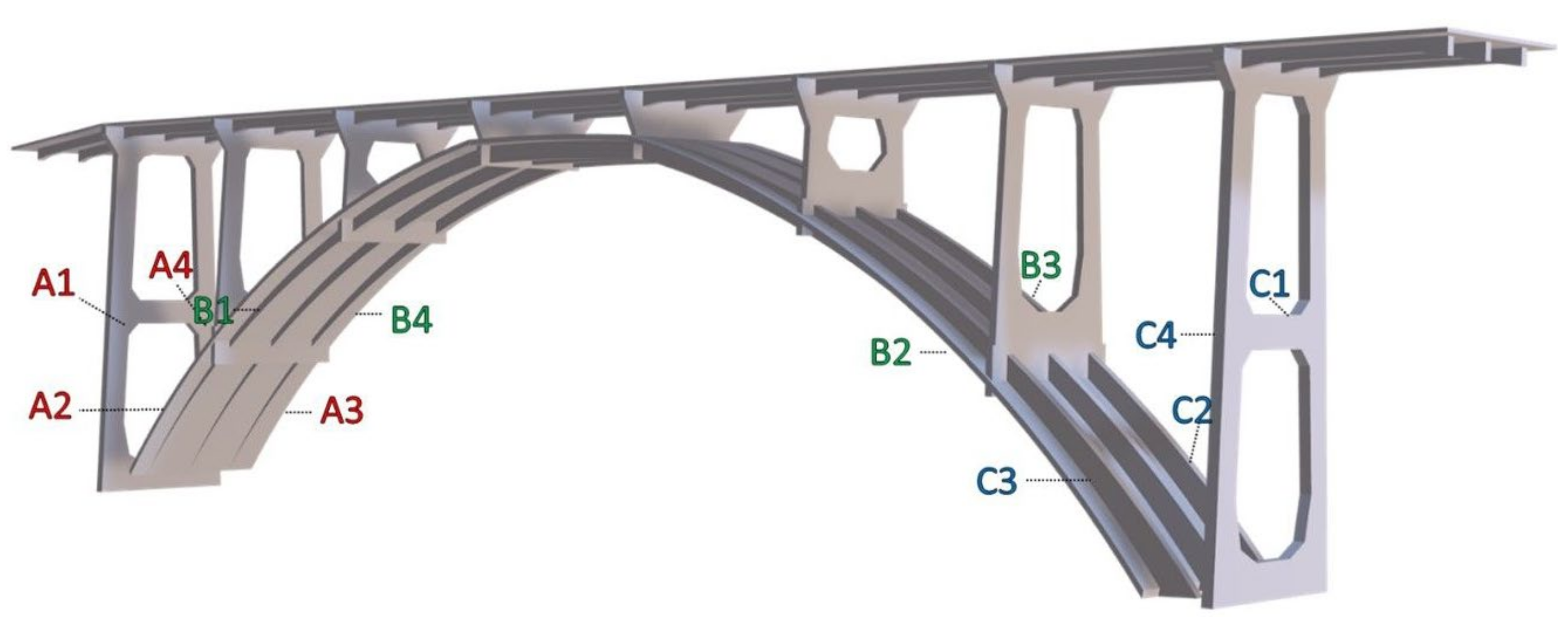
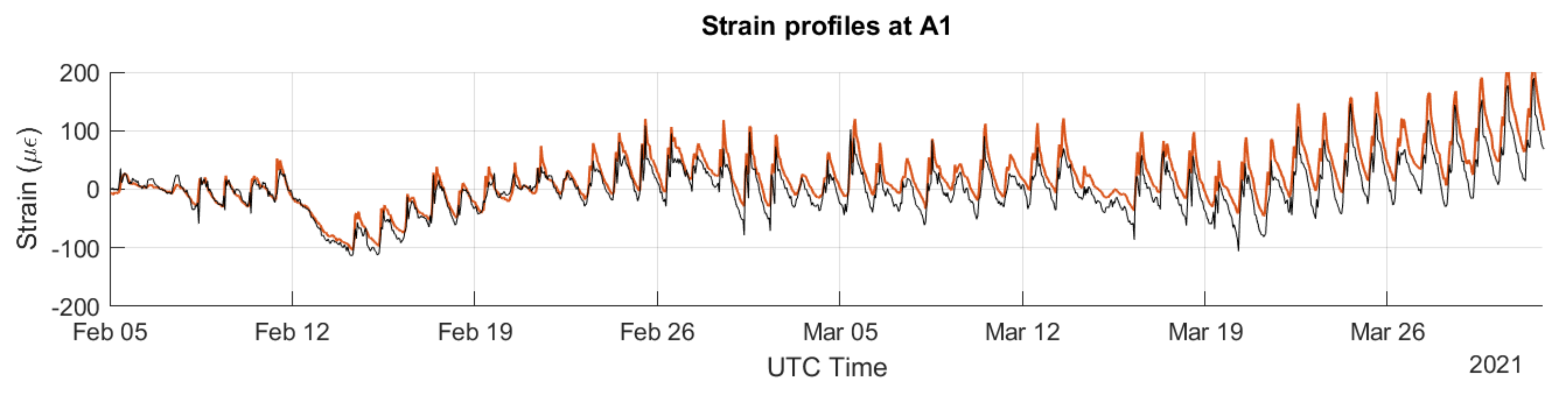
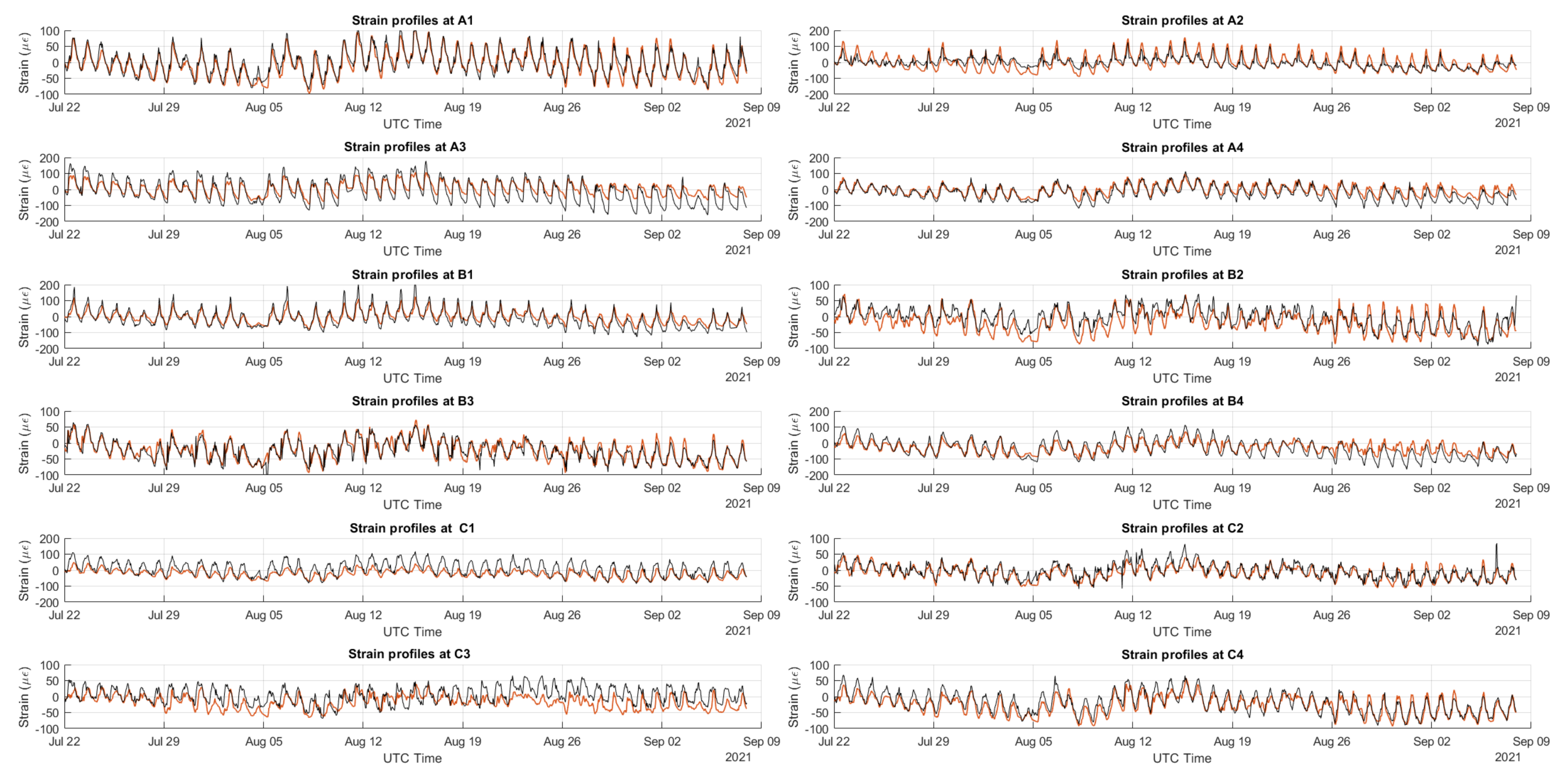
Position	Pearson’s Correlation Coefficient
A1	0.94
A2	0.80
A3	0.92
A4	0.91
B1	0.94
B2	0.82
B3	0.89
B4	0.84
C1	0.83
C2	0.85
C3	0.48
C4	0.89

) is greater than 0.80 in all sites, except for the C3. This lower value could be caused by several factors, among which is a mismatching of the corresponding point in the D-FOS system during the mapping session and/or the presence of local heterogeneities produced by the installation process.

4. Discussion and Conclusions

The work presented in this article deals with the experimentation of solutions based on Distributed Fiber Optic Sensors for SHM of strategic hydraulic infrastructures. More than 800 m of fiber optic cables were installed on the reinforced concrete members of a penstock bridge located in a mountain valley in Northern Italy. A WSN system of VW extensometers has also been used to compare the two different strain monitoring technologies. This experience allowed to develop important knowledge related to the installation of D-FOS cables on existing structures situated in a harsh and logistically complex environment. This knowledge regards both the D-FOS installation methodology to the concrete members and the D-FOS system layout design.

The analysis of strain measurements collected by D-FOS and traditional sensors shows an overall good correlation between the two series, but not a perfect coincidence. Indeed, it is important to remark that VW integrates the strain on the scale of 15 cm, leading to a substantial “punctual” measurement. In the D-FOS system instead, every sampled point integrates the BFS over to 2 m around it. Hence, D-FOS data averages the effects of local heterogeneities of the structure and that related to temperature variations: the structure’s location in a narrow mountain valley leads to extremely partial, discontinuous, and heterogeneous solar radiation conditions, even within the same day. This gives rise to relatively strong variations in the strain, even at the scale of a few meters.

For these reasons, while one is reasonably an approximation of the other, the two measures are not suitable for a rigid direct comparison. However, thanks to the presence of calibration sections A1 and A4, a series of strain measurements provided both by the strain gauge and D-FOS are available, together with temperature variations measured by temperature probes. In these sections, the strain gauge measurements have been used to optimize the calibration of the transduction coefficient $C_s$ for better measurement tailoring in a specific environmental and structural context.

Brillouin D-FOS provides a sound and accurate strain profile along extensive portions of structure members, offering a huge number of sampling points with a low cost per point. In this paper, we propose the results of an application on an aged and complex structure.

The installation method, that is the bonding of the fiber optic cable on the structure’s skin using a polyurethane adhesive, has granted a rigid transfer of the surface strain of concrete members. This method offers a non-invasive solution for existing and, like in this case, historical structures. As concerns the monitoring system as a whole, the spatial and temporal resolution depend only on the interrogator device unit: once the D-FOS cable infrastructure is installed, the system monitoring features can be subsequently changed by plugging in a different interrogator unit. In this way, the system could also be maintained and updated with the ever-changing market of Brillouin interrogators.

At the time this article is written, about five months of continuous strain measurements are available, with a temporal resolution of 30 min. As the dataset will reach a longer temporal extension, it will be interesting to analyze the thermal behavior of the structure on the seasonal scale and get the thermal strain compliance regime of the bridge itself that will be dynamically updated with time. In this way, non-conformities caused by pure mechanical stresses, whether internal or external, could be distinguished and a warning system, adequately designed, could be properly activated. The system appears to be particularly suitable for the deformative monitoring of linear infrastructures and the non-invasive installation method, practicable even in a harsh environment, allows to preserve the structural integrity of the work.

References

- Chen, H.-P. Structural Health Monitoring of Large Civil Engineering Structures; John Wiley & Sons: Hoboken, NJ, USA, 2018. [Google Scholar]
- Brownjohn, J.M.W. Structural health monitoring of civil infrastructure. Philos. Trans. R. Soc. A Math. Phys. Eng. Sci. 2007, 365, 589–622. [Google Scholar] [CrossRef] [Green Version]
- Li, H.-N.; Ren, L.; Jia, Z.-G.; Yi, T.-H.; Li, D.-S. State-of-the-art in structural health monitoring of large and complex civil infrastructures. J. Civ. Struct. Health Monit. 2016, 6, 3–16. [Google Scholar] [CrossRef]
- Farrar, C.R.; Worden, K. An introduction to structural health monitoring. New Trends Vib. Based Struct. Health Monit. 2010, 365, 303–315. [Google Scholar]
- Mays, G.C. Durability of Concrete Structures: Investigation, Repair, Protection; CRC Press: Boca Raton, FL, USA, 1991. [Google Scholar]
- Baecher, G.B.; Paté, M.E.; de Neufville, R. Risk of dam failure in benefit-cost analysis. Water Resour. Res. 1980, 16, 449–456. [Google Scholar] [CrossRef]
- Evans, J.E.; Mackey, S.D.; Gottgens, J.F.; Gill, W.M. Lessons from a Dam Failure. Ohio J. Sci. 2000, 100, 121–131. [Google Scholar]
- Sills, G.L.; Vroman, N.D.; Wahl, R.E.; Schwanz, N.T. Overview of New Orleans levee failures: Lessons learned and their impact on national levee design and assessment. J. Geotech. Geoenviron. Eng. 2008, 134, 556–565. [Google Scholar] [CrossRef] [Green Version]
- Valdez, B.; Schorr, M.; Quintero, M.; García, R.; Rosas, N. Effect of climate change on durability of engineering materials in hydraulic infrastructure: An overview. Corros. Eng. Sci. Technol. 2010, 45, 34–41. [Google Scholar] [CrossRef]
- Duratorre, T.; Bombelli, G.M.; Menduni, G.; Bocchiola, D. Hydropower Potential in the Alps under Climate Change Scenarios. The Chavonne Plant, Val D’Aosta. Water 2020, 12, 2011. [Google Scholar] [CrossRef]
- Enckell, M. Structural Health Monitoring using Modern Sensor Technology–Long-term Monitoring of the New Årsta Railway Bridge. Ph.D. Thesis, KTH Royal Institute of Technology, Stockholm, Sweden, 2006. [Google Scholar]
- Liu, Y.; Nayak, S. Structural health monitoring: State of the art and perspectives. Jom 2012, 64, 789–792. [Google Scholar] [CrossRef]
- Chopra, I. Review of state of art of smart structures and integrated systems. AIAA J. 2002, 40, 2145–2187. [Google Scholar] [CrossRef]
- Hopman, V.; Kruiver, P.; Koelewijn, A.; Peters, T. How to create a smart levee. In Proceedings of the 8th international symposium on field measurements in GeoMechanics, Berlin, Germany, 12–16 September 2011; pp. 12–16. [Google Scholar]
- Sekuła, K.; Borecka, A.; Kessler, D.; Majerski, P. Smart levee in Poland. Full-scale monitoring experimental study of levees by different methods. Comput. Sci. 2017, 18, 357. [Google Scholar] [CrossRef] [Green Version]
- De Vries, G.; Koelewijn, A.R.; Hopman, V. IJkdijk Full Scale Underseepage Erosion (Piping) Test: Evaluation of Innovative Sensor Technology. In Proceedings of the International Conference on Scour and Erosion (ICSE-5), San Francisco, CA, USA, 7–10 November 2010; pp. 649–657. [Google Scholar]
- Bertulessi, M.; Bignami, D.F.; Boschini, I.; Chiarini, A.; Ferrario, M.; Mazzon, N.; Menduni, G.; Morosi, J.; Zambrini, F. Conceptualization and Prototype of an Anti-Erosion Sensing Revetment for Levee Monitoring: Experimental Tests and Numerical Modeling. Water 2020, 12, 3025. [Google Scholar] [CrossRef]
- Barrias, A.; Casas, J.R.; Villalba, S. A review of distributed optical fiber sensors for civil engineering applications. Sensors 2016, 16, 748. [Google Scholar] [CrossRef] [PubMed] [Green Version]
- Ansari, F. Practical implementation of optical fiber sensors in civil structural health monitoring. J. Intell. Mater. Syst. Struct. 2007, 18, 879–889. [Google Scholar] [CrossRef]
- Bao, X.; DeMerchant, M.; Brown, A.; Bremner, T. Tensile and compressive strain measurement in the lab and field with the distributed Brillouin scattering sensor. J. Lightwave Technol. 2001, 19, 1698. [Google Scholar]
- Bastianini, F.; Matta, F.; Rizzo, A.; Galati, N.; Nanni, A. Overview of recent bridge monitoring applications using distributed Brillouin fiber optic sensors. J. Nondestruct. Test 2007, 12, 269–276. [Google Scholar]
- Minardo, A.; Persichetti, G.; Testa, G.; Zeni, L.; Bernini, R. Long term structural health monitoring by Brillouin fibre-optic sensing: A real case. J. Geophys. Eng. 2012, 9, S64–S69. [Google Scholar] [CrossRef]
- Ohno, H.; Naruse, H.; Kihara, M.; Shimada, A. Industrial applications of the BOTDR optical fiber strain sensor. Opt. Fiber Technol. 2001, 7, 45–64. [Google Scholar] [CrossRef]
- Menduni, G.; Viani, F.; Robol, F.; Giarola, E.; Polo, A.; Oliveri, G.; Rocca, P.; Massa, A. A WSN-based architecture for the E-Museum-the experience at ‘Sala dei 500′ in Palazzo Vecchio (Florence). In Proceedings of the 2013 IEEE Antennas and Propagation Society International Symposium (APSURSI), Orlando, FL, USA, 7–13 July 2013; pp. 1114–1115. [Google Scholar]
- Motil, A.; Bergman, A.; Tur, M. State of the art of Brillouin fiber-optic distributed sensing. Opt. Laser Technol. 2016, 78, 81–103. [Google Scholar] [CrossRef]
- Ansari, F.; Libo, Y. Mechanics of bond and interface shear transfer in optical fiber sensors. J. Eng. Mech. 1998, 124, 385–394. [Google Scholar] [CrossRef]
- Montero, W.; Farag, R.; Diaz, V.; Ramirez, M.; Boada, B.L. Uncertainties associated with strain-measuring systems using resistance strain gauges. J. Strain Anal. Eng. Des. 2011, 46, 1–13. [Google Scholar] [CrossRef]
- Bastianini, F.; di Sante, R.; Falcetelli, F.; Marini, D.; Bolognini, G. Optical fiber sensing cables for Brillouin-based distributed measurements. Sensors 2019, 19, 5172. [Google Scholar] [CrossRef] [PubMed] [Green Version]
- Zou, W.; He, Z.; Hotate, K. Complete discrimination of strain and temperature using Brillouin frequency shift and birefringence in a polarization-maintaining fiber. Opt. Express 2009, 17, 1248–1255. [Google Scholar] [CrossRef] [PubMed]
- Mohamad, H.; Soga, K.; Amatya, B. Thermal strain sensing of concrete piles using Brillouin optical time domain reflectometry. Geotech. Test. J. 2014, 37, 333–346. [Google Scholar] [CrossRef]
- Lanticq, V.; Quiertant, M.; Merliot, E.; Delepine-Lesoille, S. Brillouin sensing cable: Design and experimental validation. IEEE Sens. J. 2008, 8, 1194–1201. [Google Scholar] [CrossRef]
- Lanciano, C.; Salvini, R. Monitoring of strain and temperature in an open pit using Brillouin distributed optical fiber sensors. Sensors 2020, 20, 1924. [Google Scholar] [CrossRef] [Green Version]
- Neild, S.A.; Williams, M.S.; McFadden, P.D. Development of a vibrating wire strain gauge for measuring small strains in concrete beams. Strain 2005, 41, 3–9. [Google Scholar] [CrossRef]
- Furgale, P.; Rehder, J.; Siegwart, R. Unified temporal and spatial calibration for multi-sensor systems. In Proceedings of the 2013 IEEE/RSJ International Conference on Intelligent Robots and Systems, Tokyo, Japan, 3–7 November 2013; pp. 1280–1286. [Google Scholar]