
Longitudinal River Monitoring and Modelling Substantiate the Impact of Weirs on Nitrogen Dynamics


Department of Hydro Sciences, Faculty of Environmental Sciences, Institute of Urban and Industrial Water Management, TU Dresden, 01069 Dresden, Germany
*
Author to whom correspondence should be addressed.
Water 2022, 14(2), 189; https://doi.org/10.3390/w14020189
Submission received: 29 October 2021
/
Revised: 20 December 2021
/
Accepted: 31 December 2021
/
Published: 10 January 2022
(This article belongs to the Section Water Quality and Contamination)
Abstract
:The fluvial nitrogen dynamics at locations around weirs are still rarely studied in detail. Eulerian data, often used by conventional river monitoring and modelling approaches, lags the spatial resolution for an unambiguous representation. With the aim to address this knowledge gap, the present study applies a coupled 1D hydrodynamic–water quality model to a 26.9 km stretch of an upland river. Tailored simulations were performed for river sections with water retention and free-flow conditions to quantify the weirs’ influences on nitrogen dynamics. The water quality data were sampled with Eulerian and Lagrangian strategies. Despite the limitations in terms of required spatial discretization and simulation time, refined model calibrations with high spatiotemporal resolution corroborated the high ammonification rates (0.015 d−1) on river sections without weirs and high nitrification rates (0.17 d−1 ammonium to nitrate, 0.78 d−1 nitrate to nitrite) on river sections with weirs. Additionally, using estimations of denitrification based on typical values for riverbed sediment as a reference, we could demonstrate that in our case study, weirs can improve denitrification substantially. The produced backwater lengths can induce a means of additional nitrogen removal of 0.2-ton d−1 (10.9%) during warm and low-flow periods.
1. Introduction
The European Water Framework Directive (WFD) stipulated that by 2027 at the latest, all surface water bodies (e.g., lakes, rivers, coastal waters) must achieve good ecological and chemical status [1]. However, only 40% of approximately 111,000 surface water bodies across Europe have so far fulfilled the WFD objective [2]. Monitoring programs are an essential part of WFD management cycles and they provide the key basis for ecological and chemical status assessment. River Basin Management Plans (RBMP) report status deficits caused by pollution and hydromorphological pressures, and they propose and prioritize different restoration measures [2,3,4].
River pollution pressures include emissions of nutrients, organic matter and hazardous chemicals from diffuse and point sources (e.g., agriculture, sewage system discharges). Nitrogen (N) is one of the most vital nutrients for plant growth. Despite its key role for increasing crop production, it is also considered as main pollutant for aquatic and terrestrial ecosystems [5,6]. Over past centuries, anthropogenic activities have markedly modified and intensified the natural N cycle. Massive production and application of fertilizers have led to continuous excess N in soil and water, which results in other harmful processes such as soil acidification and eutrophication [7,8].
In aquatic systems, the following transformation processes control N occurrence, among others: the mineralization and hydrolysis reactions of organic matter to ammonia release, two-step oxidation of ammonia to nitrite and nitrate (nitrification) and reduction of nitrate to gaseous nitrogen under anaerobic conditions (denitrification) along with nitrate uptake by nitrogen-fixing algae [9]. Although most conventional river quality models can simulate N transformation processes in simplified ways, model calibrations are often constrained to fixed measuring points along the river [9,10,11]. This monitoring approach corresponds to a Eulerian specification of the flow [10], from which statements about longitudinal development of river nutrient dynamics based on point data can be uncertain. Alternatively, longitudinal river monitoring, which corresponds to the Lagrangian specification of the flow [10], are a promising approach to overcome such limitations. They spatially specify substance concentrations and transformation processes [12]. Site-specific water quality coefficients (e.g., N turnover rates) can be refined and regionalized with measurements along a flowing wave [13]. If required, the results from existing Eulerian river quality models can be transformed into the Lagrangian system to perform spatiotemporal calibration [10].
On the other hand, the measuring and modelling of river denitrification remain vexing and difficult at large spatial scales because of the complex reactions taking place at the interface between the water column and the riverbed sediment, as well as in the adjacent riparian wetlands [14,15,16]. While some conventional river quality models omit denitrification conservatively [11,17,18], other enhanced models have coupled submodules to include benthic and riparian zones for denitrification modelling [11,19,20,21,22]. Nevertheless, these model enhancements are dependent on detailed information of particulate material and organic matter within the benthic sediment layers at the required spatial scale, which is normally rarely available [20]. Alternatively, previous studies proposed model adaptation methods [19,20,22] or post-processing modelled nitrate concentrations to take into account river denitrification. For this latter approach, strong relationships between denitrified nitrate with hydraulic depth and water residence time were evidenced [14,23,24].
River hydromorphological pressures refer to human physical alterations (e.g., channelization, dams, weirs), which affect significantly the river hydraulic regime, continuity and morphology [2,4,25]. A widespread restoration measure in over two-thirds of European river basins is related to the removal of transversal structures (e.g., weirs) to meet the WFD ecological goals [4,24]. The main pressure produced by weirs on rivers is the disruption of the longitudinal integrity of running waters. They impair the physicochemical balance along the river by interfering with sediment and nutrient transport by the formation of impoundment and erosion areas as well as diminishing the habitat diversity and migration of fish and other aquatic species [26,27]. In spite of that, weirs also provide other significant services such as flow gauging, water level regulation in terms of flood control, recreation and food for people, aeration to downstream river sections and nutrient cycling [20,24]. With regard to the last point, the water retention conditions produced by weirs promote the diminishment of nutrient export to downstream river sections through mainly particle settling and denitrification processes [28,29]. However, the significance of the partial loss of this nutrient sink function by restoring rivers through weir removal is still not well defined for large river sections [24,29] since most studies were especially performed in very short river sections or for specific hydraulic structures in case of N removal [23].
In this study, we aim to identify and quantify detailed spatiotemporal N turnover patterns under the influence of weirs along a 26.9 km section of an upland river in eastern Germany, the Freiberger Mulde. For this purpose, refined 1D water quality model calibrations within the time period 2017–2018 were conducted using both fixed (Eulerian) measurements from water quality stations within the framework of WFD complemented with longitudinal (Lagrangian) measurements from independent boat-based sampling campaigns with high spatial resolution. For quantification and assessment of the weirs’ effect on fluvial nitrogen dynamics, multiple simulations at different river sections with water retention conditions (weirs present) and free-flow conditions (without weirs) using their corresponding N turnover rates were performed and separately analyzed. At the same time, the site-specific characteristic values of N removal were determined to quantify and to compare explicitly the denitrification performance at current river conditions (weirs present) and the hypothetical scenario representing the removal of weirs.
Although uncertainty analysis under Monte Carlo [30] or generalized likelihood un-certainty estimation (GLUE) [31] methods is generally desired on results of complex environmental simulations, it may become computationally challenging when models of long river sections require very fine spatiotemporal discretization, as is the case for this study. This limitation is addressed through a sensitivity analysis of spatial discretization and computation time to estimate to what extent the findings can be considered satisfactory.
2. Materials and Methods
2.1. Study Area
With a total length of 124 km, 0.58% mean slope and a catchment drained area (CDA) of 2985 km2, the Freiberger Mulde (FM) is a large mid-altitude siliceous river [32]. The headwater source of FM river is located in the Czech Republic (around 5 km from the German border) and it flows northwest across the German Free State of Saxony. The land use of FM river catchment is dominated by crop fields (40%), forests (30%) and grasslands (18%) [33]. Around 78% of the total length of the FM river has moderate pollution from oxygen-depleting organic substances [34]. Estimated total nitrogen load at FM mouth and total nitrogen retention reach 6052-ton yr−1 and 16.2%, respectively [35,36]. In addition, the FM river shows high concentrations of heavy metals (As, Cd, Cu, Ni, Pb, Zn) in sediment caused by geogenic and anthropogenic activities in upper subcatchments [32,37,38,39].
According to German navigation, the FM river stationing starts at the river mouth and ends at the Czech–German border. The river course passes through urban populations with a connection degree >70% to wastewater treatment plants (WWTP) whose outlets discharge directly into the FM river [40,41]. Mean annual rainfall is 663.2 mm (climate station Nossen, 51.06° N 13.27° E) [42] and mean annual discharge (MQ) is 29.1 m3 s−1 (water gauge Leisnig, FM-km 13.6) [43]. The longitudinal continuity of FM mainstream is heavily disturbed by 28 weirs. Most of them are used for hydropower and flow regulation [44].
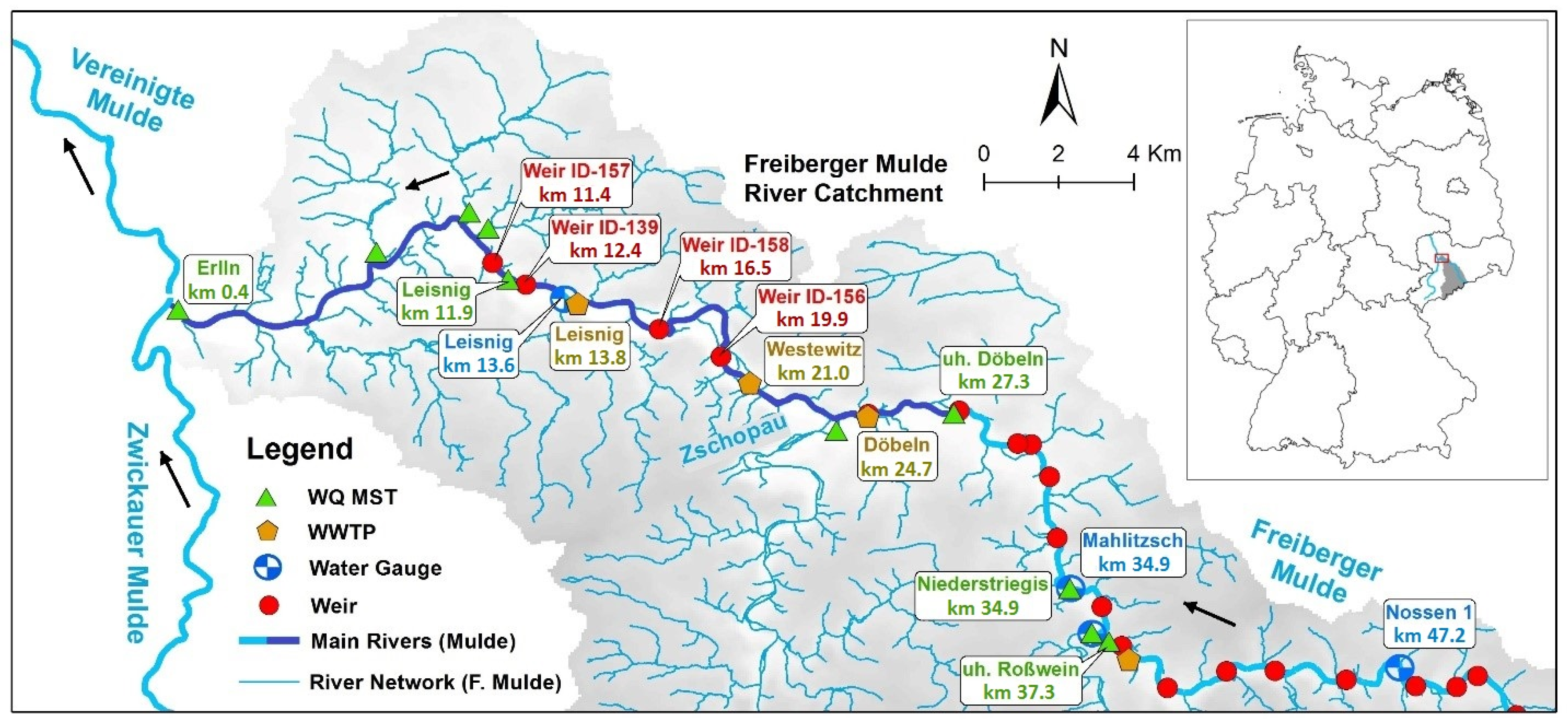
The study area is located in the lowermost part of FM river (Figure 1). The section between river mouth (FM-km 0) and water gauge Nossen 1 (ID: 566040, FM-km 47.2) provided hydrodynamic boundary conditions, whereas the 26.9 km river section between the water quality monitoring stations (WQMST) uh. Döbeln (ID: 32000, FM-km 27.3) and Erlln (ID: 32300, FM-km 0.4) was repeatedly probed during the longitudinal boat-based sampling campaigns in 2017–2018 [45]. The investigated FM river section covers a subsection with flow retention conditions due to weirs (from Döbeln to Leisnig), a subsection with free-flow conditions (from Leisnig to Erlln) and the input of Zschopau River, the main tributary of FM river. Other identified inputs to the FM river include 18 small tributaries and three WWTP: Döbeln (FM-km 24.7), Westewitz (FM-km 21.0) and Leisnig (FM-km 13.8) with a total size of 52,500 as population equivalent.
2.2. Model Description
Model simulations were carried out by the model HEC-RAS 5.0.3 (Hydraulic Engineering Center–River Analysis System)—an integrated and open-source software developed by the Institute of Hydrologic Engineering Center of the US Army Corps. It allows detailed and accurate 1D steady and unsteady flow simulations of natural and constructed channels including backwater effects related to any kind of in-stream structures (e.g., weirs). It robustly solves the Saint-Venant equations with an implicit finite difference method [46]. Additionally, HEC-RAS is coupled with the water temperature and nutrient simulation module (NSM-I), which is based on the principle of mass balance [17].
The NSM-I module calculates the major transformation processes of water quality variables within the water column by solving the 1D-adversion-dispersion equation with the explicit numerical scheme Quickest–Ultimate [47]. As descendant of former well-known water quality models such as QUAL2K and CE-QUALRIV1, the coupled HEC-RAS-NSM-I model is capable of simulating, among other water quality variables, phytoplankton algae (algae) or chlorophyll-a (Chl-a), dissolved oxygen (DO), organic nitrogen fraction (Org-N) and inorganic nitrogen forms (Inorg-N): nitrate nitrogen (NO3-N), nitrite nitrogen (NO2-N) and ammonium nitrogen (NH4-N); meanwhile water temperature is implemented using a full energy budget approach [17,18,21]. Both input and output time series are stored in HEC-DSS files. The HEC-DSS (Data Storage System) is a database system designed to efficiently store and retrieve time-based sequential data [48].
2.3. Data Collection and Preparation
The primary collection of input data for different model configurations with HEC-RAS-NSM-I was extracted from official databases (Eulerian measurements) and from longitudinal boat-based sampling databases (Lagrangian measurements). Their sources are summarized in Appendix A. River geometry was represented through 246 georeferenced topographic profiles of cross sections and 15 weir elevation profiles located in the study area. They were obtained from a survey conducted by the regional State Dam Administration within the framework of flood risk management for the FM river catchment. The river channel cross sections were extended with river overbanks by using a digital elevation model with 2 m grid size.
Eulerian hydraulic data (e.g., flow discharge, water stage) with 15 min/daily resolution and water quality data (e.g., concentrations of N forms) with daily/monthly resolution were extracted from fixed water gauges and WQMST, which belong to a regional monitoring program developed for all Saxonian rivers. These datasets have public access through an interdisciplinary data portal provided by the regional environmental authority [49]. In addition, daily measurements of hydraulic and water quality parameters at WWTP effluents outlets were retrieved from hand-written WWTP operation booklets. For water temperature modelling, hourly meteorological data from official climate stations Nossen (51.06° N 13.27° E) and Dürrweitzschen (51.2° N 12.86° E) were applied [42].
Indirect estimations of non-measured algae concentrations were derived from calculations of Redfield stoichiometric weight ratios (Equation (1)) [21,50]. Furthermore, it is assumed that ultimate CBOD and modified CBOD5 follow the exponential first-order kinetics of dissolved organic carbon (DOC) oxidation (Equations (2) and (3)) according to [51].
where: C = carbon, N = nitrogen, P = phosphorus, Chl-a = chlorophyll-a, = 5-day carbonaceous biochemical oxygen demand (mg L−1), = ultimate carbonaceous biochemical oxygen demand (mg L−1), = dissolved organic carbon (mg L−1), = DOC oxidation rate (0.01 d−1 for rivers), = CBOD oxidation rate (0.02 d−1 for rivers), = O2:C ratio for carbon oxidation (2.667 mg-O2 mg-C−1).
100.0 g Algae: 40 g C : 7.2 g N : 1.0 g P : (0.4 − 1.0) g Chl-a
For the Lagrangian calibration strategy, three longitudinal sampling campaigns were performed along the 26.9 km section of FM river between WQMST uh. Döbeln and WQMST Erlln within the framework of the German research project BOOT-Monitoring. They took place during summer and autumn (15 August 2017, 12 October 2017, 9–11 July 2018). Among other parameters, concentrations of NO3-N, total organic carbon (TOC) and dissolved organic carbon (DOC) were measured by spectrophotometer (s::can spectrolyzer, s::can GmbH, Vienna, Austria) and ion-selective probes (MPS-D8, SEBA Hydrometrie GmbH & Co. KG, Kaufbeuren, Germany) coupled to a boat-based measuring system. The time resolution of raw measurements was less than one second, but they were averaged every minute for modelling and calibration purposes. Further detailed information about the conception and configuration of the boat-based measuring system can be found in [45,52]. Non-measured longitudinal concentrations of N forms (Total-N, Inorg-N and NO2-N) were estimated by regressions obtained with data from WQMST located in the study area (Figure 2). Furthermore, mass balance calculations were applied to estimate NH4-N concentration (Equation (4)) and Org-N concentration (Equation (5)).
Inorg-N = NO3-N + NO2-N + NH4-N
Total-N = Inorg-N + Org-N
2.4. Nitrogen Modelling and Calibration with HEC-RAS-NSM-I
The hydrodynamic setup comprised the implementation of geometric data of river cross sections collected for the river section between FM river mouth and water gauge Nossen 1 along with complementary hydraulic information on downstream reach lengths, contraction/expansion coefficients, Manning roughness coefficients (n), weir crest shapes, weir widths and weir flow coefficients. Since hydrodynamic calculations with HEC-RAS are less accurate if cross sections are too far apart from each other [53], the surveyed river cross sections were interpolated into an average spacing interval of 25 m to avoid model instabilities. The embedded interpolation tool in HEC-RAS is based on a string model that connects coordinates and elevation points of upstream and downstream cross sections through curvilinear shapes by following the horizontal alignments of river main channel and river overbanks. The discharge hydrograph at flow gauge Nossen 1 with 15 min temporal resolution defines the upstream hydraulic boundary condition. Lateral discharge inflows were implemented by location along the river longitudinal stationing. They included both WWTP effluent outlets and interpolated flow discharges of small tributaries of FM river. This later interpolation was performed based on regionalized weighted CDA and flow time lags of discharge peaks along the FM river flow path. With simulations of 15 min computation time steps and using the Manning roughness coefficient as a calibration parameter within the ranges given by [54], the hydrodynamic HEC-RAS model was calibrated with the measured discharge data at water gauges Mahlitzsch (ID: 566055, FM-km 34.9) and Leisnig (ID: 566085, FM-km 13.6) for the time period 2017–2018.
Once the hydrodynamic model was calibrated, the calculated values of flow discharge, flow velocity and hydraulic depth were transferred to water quality cells created in the NSM-I module between the river cross sections. For each water quality cell, the advection–dispersion and heat exchange equations given by [18,21,47] are solved with 15 min computation time steps. Here, the upper boundary condition of N modeling is given by the time series of water quality parameters at WQMST uh. Döbeln. Lateral inputs were extracted from measurements of existing WWTP effluent discharges and WQMST located at tributary rivers shortly before their mouths into FM river: WQMST Pischwitz (Zschopau River, ID: 35350, FM-km 23.7), WQMST Mündung 201 (Goernitzbach River, ID: 32201, FM-km 10.5), WQMST Polkenmühle (Polkenbach River, ID: 32203, FM-km 10.0) and WQMST Mündung 205 (Fritzschenbach River, ID: 32205, FM-km 6.8). Lateral inputs of other small tributaries in the study area were derived from average values of WQMST located at corresponding nearest tributaries. Eulerian model calibration of turnover rates of water quality constituents (e.g., N forms) for the time period 2017–2018 was performed using measured data at WQMST Leisnig (ID: 32200, FM-km 11.9) and at WQMST Erlln (ID: 32300, FM-km 0.4) located at the downstream ends of FM river sections with water retention (weirs present) and free-flow conditions (without weirs), respectively.
Complementary, longitudinal water quality data from independent boat-based sampling campaigns (15 August 2017, 12 October 2017, 9–11 July 2018) were implemented with the aim to refine the water quality calibration parameters (e.g., N turnover rates). The high temporal resolution of computation time step (1 min) of HEC-RAS-NSM-I model enabled accurate spatiotemporal alignment of modelled and measured values. For Lagrangian calibration setups at each investigated river section, average water quality values measured at the uppermost part constituted the upstream boundary conditions for each boat-based sampling campaign. Consequently, the upstream boundary condition for the river section influenced by weirs was located at FM-km 24.2 (shortly upstream of the inflow of Zschopau tributary river) and the upstream boundary condition for the river section with free-flow conditions was located at FM-km 10.0. Lateral concentration and load inputs were determined by local mass balance calculations from measurements before and after each point source (e.g., tributary river and WWTP effluent). Lagrangian model calibrations of N turnover rates were conducted through R-scripts for the comparison between measured and modelled values stored in HEC-DSS files.
Since the boat-based measuring system provided a high longitudinal density of measurements, Lagrangian calibration setups enabled higher spatial discretization of average spacing between cross sections (2–10 m) than Eulerian calibration setups. By default, the latter creates small water quality cells, which are prone to numerical instabilities and very long computation time. To overcome this, the HEC-RAS-NSM-I model allows us to combine water quality cells with the caution of losing accuracy of modelling results [17]. Consequently, a sensitivity analysis (described below) was performed to show the influence of spatial model discretization on computation time and multiple calibration performance.
2.5. Evaluation of Model Calibration Performance
The calibration performance of hydrodynamic and water quality simulations was evaluated with goodness-of-fit indices recommended by [55], where hydrodynamic and water quality simulations can be considered satisfactory if they achieve simultaneously the Nash Sutcliffe Efficiency coefficient (NSE) > 0.50, the ratio of root mean square error to standard deviation (RSR) < 0.70 and the relative percentage error (% PBIAS) < ±25% (for flow discharges) or <±70% (for water quality parameters). Additionally, the widely known root mean square error (RMSE) was included for assessing the calibration performance against observed data with very low spatial variability (e.g., boat-based measurements). RMSE values close to zero indicate optimal model fitting [55].
2.6. Sensitivity Analysis of Spatial Discretization with HEC-RAS-NSM-I
A sensitivity analysis of spatial discretization was performed using different lengths of combined water quality cells (from 2 m to 500 m) for Eulerian calibration (time period 2017–2018) and Lagrangian calibration (boat-based sampling campaigns 15 August 2017 and 9–11 July 2018). In order to optimize the tradeoff between computation time and model accuracy, maximum lengths of combined water quality cells for satisfactory calibration were determined according to the criteria mentioned above. Implications of computation time for a full uncertainty assessment within frameworks of Monte Carlo [30] or generalized likelihood uncertainty estimation (GLUE) [31] were evaluated. Model simulations were conducted on an Intel Core i7-7600, 2.9 GHz processor.
2.7. Quantification of River Denitrification Dynamics
In view of the complexity involved to direct quantification of fluvial denitrification, previous studies of river catchments observed a strong relationship between denitrification processes occurring at river bed/water column interface and hydraulic depth. Approaches for calculation of N removal varied, depending on using concentration values of dissolved Inorg-N forms, Total-N [23] or nitrogen gas (N2) [56]. Complex nitrate reduction processes are usually described by denitrification rates following the first-order kinetics (Equation (6)) along the corresponding river section [14,24,57,58].
where: = nitrate concentration at downstream of a given river section i, = nitrate concentration at upstream of a given river section i, = denitrification rate of a given river section i, = flow travel time along a given river section i.
Additionally, empirical evidence from different UK river basin studies [14,24] provided a modified version to calculate denitrification rates by considering the spatial variability of riverbed sediment characteristics and hydraulic loads using Equation (7).
where: = characteristic constant for riverbed sediment at a given river section i ( = 0.05 found in UK rivers studies), = hydraulic depth at a given river section i, = water temperature at a given river section i.
With the purpose of estimating and comparing the potential denitrification along the FM river sections with weirs present (from Döbeln to Leisnig) and without influence of weirs (from Leisnig to Erlln), local denitrification rates were obtained with Equation (6) using longitudinal nitrate concentrations measured during the boat-based sampling campaigns and hydraulic values calculated by the hydrodynamic HEC-RAS model. Subsequently, mean site-specific constants () of riverbed sediments were calculated with Equation (7) at each corresponding FM river section. For the FM river sections with water retention conditions due to weirs (between FM-km 11.4 and FM-km 23.5), two scenarios were implemented to quantify the weirs’ influence on long-term fluvial denitrification for the time period 2017–2018. In the first place, the current state scenario (weirs present) consisted of simulation and quantification of denitrification using the calibrated N turnover rates and the corresponding riverbed sediment constants (). The second scenario evaluated the hypothetical removal of weirs: Weir ID-156 (FM-km 19.9), Weir ID-158 (FM-km 16.5), Weir ID-157 (FM-km 12.4) and Weir ID-139 (FM-km 11.4). Here, coupled hydrodynamic and water quality simulations were performed with N turnover rates determined for an FM river section without weirs (between FM-km 0.0 and FM-km 10.0). In the same way, riverbed sediment constants () for FM river section without weirs were used to quantify denitrification. Comparison of both scenarios (weirs present and without weirs) in terms of depletion of NO3-N concentrations and NO3-N loads were analyzed in detail.
3. Results and Discussion
3.1. Hydrodynamic Model Calibration Using High-Resolution Flow Data
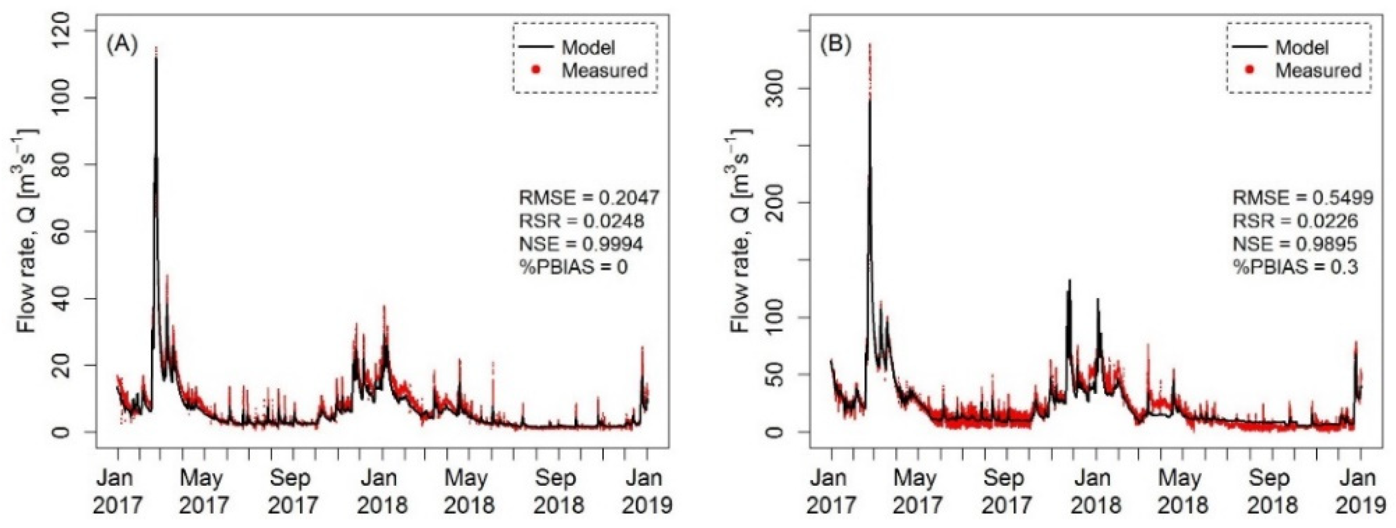
Very good hydrodynamic calibration performance was achieved at intermediate water gauges Nossen 1 and Mahlitzsch with goodness-of-fit indices of RSR < 0.03, NSE > 0.98 and absolute %PBIAS < 0.35% (Figure 3). Mean values of Manning’s coefficients of n = 0.0375 for the river channel bed and n = 0.0675 for river channel slopes and river overbanks were determined. The Zschopau tributary river causes the high difference of flow rate between water gauge Mahlitzsch (MQ = 9.9 m3 s−1) and water gauge Leisnig (MQ = 30.6 m3 s−1), since its CDA covers around 57% of the CDA of the entire FM river. For the time period 2017–2018, the flow rate of the Zschopau tributary river increased on average the flow rate of the FM river by factors of 2.4 and 3.1 during winter and summer months, respectively.
With the calibrated hydrodynamic model, customized simulation runs were subsequently performed to extract hydraulic variables (flow discharge, flow velocity and hydraulic depth) at multiple spatiotemporal resolutions. These provided boundary conditions for the calibration of water quality parameters (e.g., N forms) at both FM river sections (with weirs and without weirs) using HEC-RAS-NSM-I model with Eulerian measured data from WQMST and Lagrangian measured data from boat-based sampling campaigns.
3.2. Eulerian Calibration with HEC-RAS-NSM-I Model
Turnover rates and conversion ratios of water quality constituents of the HEC-RAS-NSM-I model were calibrated iteratively with data at fixed WQMST Leisnig and WQMST Erlln (Table 1) according to recommended ranges of values summarized in [21]. For both types of river sections, equal characteristic values related to DO, CBOD and algae were determined: sediment oxygen demand (0.2 d−1), atmospheric reaeration (0.5 d−1), algal photosynthesis rate (1.8 mg-O mg-Algae−1), algal respiration (1.7 mg-O mg-Algae−1), CBOD oxidation (0.02 d−1), CBOD settling (0.00 d−1), nitrification inhibition factor (KNR = 0.65 mg L−1), maximum algal growth rate (1.0 d−1), algal settling rate (0.1 m d−1) and the fraction of algal biomass that is nitrogen (0.09 mg-N mg-Algae−1). In contrast, different turnover rates between N forms were found for each type of FM river sections. Slow-flow conditions produced by weirs evidenced significant effects on low Org-N decay rate to NH4-N (0.003 d−1, at WQMST Leisnig) in accordance with the negative relationship between organic matter decomposition and water retention time across water systems observed in a previous study [59]. Furthermore, slow-flow river sections within a system are prime locations for enhancing nitrification, since nitrifying bacteria are slow-growing organisms [60,61]. This is represented with higher oxidation rates of NH4-N to NO2-N (0.290 d−1) and NO2-N to NO3-N (0.710 d−1) calibrated at WQMST Leisnig in comparison with oxidation rates of NH4-N to NO2-N (0.150 d−1) and NO2-N to NO3-N (0.550 d−1) calibrated at WQMST Erlln.
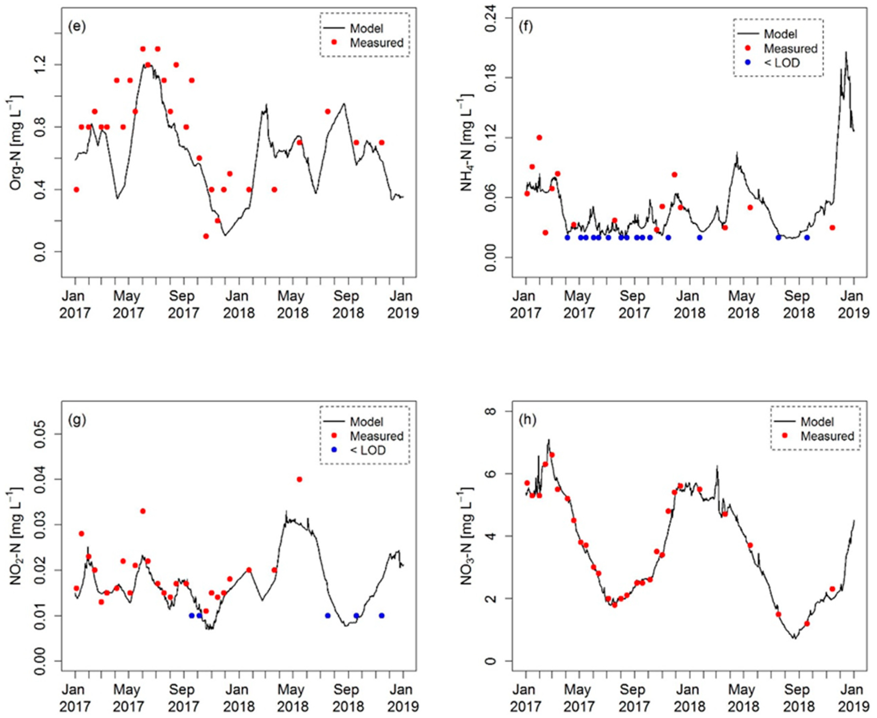
Using the calibrated turnover rates for the time period 2017–2018, modelled time series plots of N forms, DO, CBOD, algae and water temperature at WQMST Leisnig and WQMST Erlln are depicted in Figure 4 and Figure 5, respectively. The model was able to capture very well the seasonal trends of all selected water quality constituents at both WQMST, although one-to-one agreement of some predicted peak values with sampling measurements was not always possible. Concentrations of algae, Org-N and CBOD were found low during winter months until temperature and light conditions within the water column allow algal growth followed by algal decay and an increase of consumed oxygen, as described in [18]. Mean concentrations were determined for algal biomass (summer: 4.6 mg L−1; winter: 2.3 mg L−1), Org-N (summer: 0.7 mg L−1; winter: 0.5 mg L−1) and CBOD (summer: 1.4 mg L−1; winter: 1.2 mg L−1). In contrast, high NO3-N concentrations were determined during winter months. Nitrate removal may be inhibited by high-flow velocities in the river system [62] or low water temperature [63]. Mean NO3-N concentrations oscillated between 2.3 mg L−1 (summer) and 4.7 mg L−1 (winter). DO exhibited a similar seasonal pattern due to its strong relation with water temperature. Mean DO concentrations oscillated between 10.6 mg L−1 (summer) and 12.0 mg L−1 (winter). Furthermore, low concentrations of NH4-N (<0.20 mg L−1) and NO2-N (<0.04 mg L−1) were observed in both studied FM river sections during the time period 2017–2018.
In regard to the model calibration performance, the recommended goodness-of-fit indices by [55] were mostly fulfilled, except for Org-N at WQMST Leisnig (Table 2). The absolute %PBIAS error accounted for less than 30% for all selected model parameters. Simulated water temperature and NO3-N performed the best (NSE > 0.95 and RSR < 0.15); while simulated algae, Org-N (at WQMST Erlln), NH4-N and NO2-N reached lower, but acceptable performance values (NSE = 0.53 − 0.63 and RSR = 0.60 − 0.68). The decrease of these model performance indices can be attributed to low spatiotemporal resolution or shortage of direct measured data together with some limitations of HEC-RAS-NSM-I model to describe accurately organic water quality variables. For instance, HEC-RAS-NSM-I model only permits one algae group (phytoplankton) within the water column [17,18]. Moreover, the “observed” algal biomass was derived from stoichiometric correlations with organic carbon concentrations and Chl-a. This drawback by simulating algae could also have biased the simulation performance of Org-N, especially at peak values. On the other hand, optimal model fitting of NH4-N and NO2-N concentrations during the simulation time period 2017–2018 was partially not possible (NSE = 0.45 − 0.55 and RSR = 0.65 − 0.72) since few values higher than limit of detection (LOD) were used for the comparison. Nevertheless, the modelled concentration profiles of NH4-N and NO2-N fairly reproduced low concentrations in the regions where measurements less than LOD were detected.
3.3. Lagrangian Calibration with HEC-RAS-NSM-I Model
Using Lagrangian calibration setups with 50–100 m length of combined water quality cells for both FM river sections under study (with weirs and without weirs), N transformation processes were represented more explicitly by refining the N turnover rates according to boat-based measured data from sampling campaigns (15 August 2017, 12 October 2017, 9–11 July 2018) and data derived from regressions according to Section 2.3. Turnover rates related to DO, CBOD and algae shown in Table 1 were for both river sections validated and incorporated into the Lagrangian calibration setup. The longitudinally and refined calibrated turnover rates of N forms are shown in Table 3.
The turnover rates of algae N content (0.090 mg-N mg-Algae−1) and Org-N settling rate (0.005 d−1) determined in the Eulerian calibration served as the base condition for both FM river sections. The weirs’ influence on the remaining N transformation processes was corroborated by the decrease in the Org-N decay rate (from 0.015 to 0.003 d−1) and the increase in the oxidation rates of NH4-N to NO2-N (from 0.13 to 0.17 d−1) and NO2-N to NO3-N (from 0.52 to 0.78 d−1).
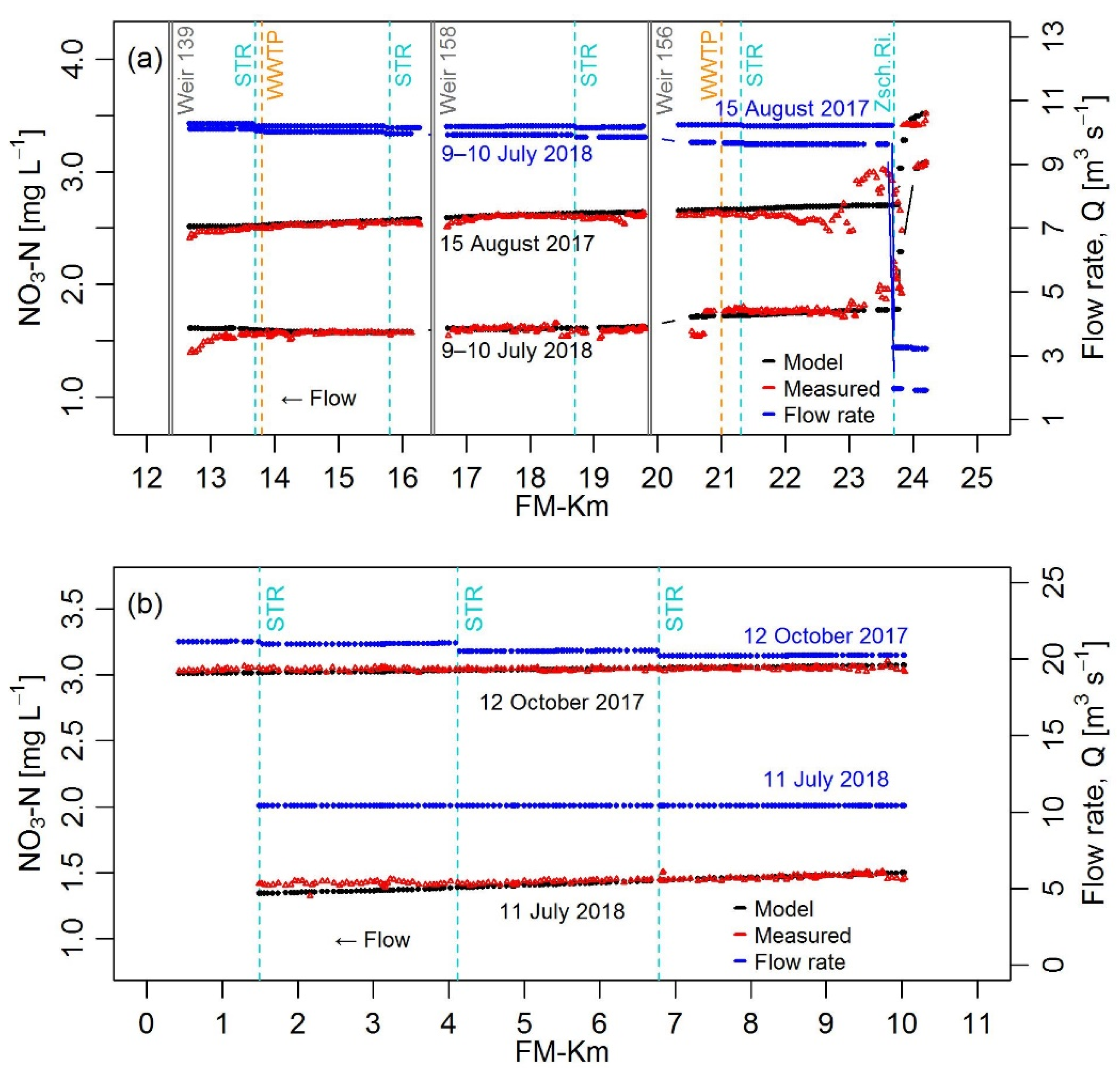
Calibration performance in both river sections achieved very good absolute fitting indices (Table 4) and reproduced the longitudinal course of nitrogen constituents consistently. Computed values of %PBIAS were found to be less than ± 2.5%, NSE higher than 0.5 and RMSE less than 0.09 (except for algae). As NO3-N was the only nitrogen constituent measured directly, examples of longitudinal concentration profiles of NO3-N are illustrated in Figure 6. From measured and modelled NO3-N concentrations around the inflow of the tributary river Zschopau, dilution processes were evident through the significant reductions of NO3-N concentrations by 25–40%. Conversely, NO3-N loads from existing WWTP and from other small tributary rivers, as well as the possible additional input of groundwater or base flow were found negligible during the days of boat-based sampling campaigns. As also reported in [24], the water retention of weirs exhibited effects on NO3-N removal by decreasing NO3-N concentrations up to 10% over a 12.1 km river section with sharp reductions of NO3-N concentrations at locations immediately upstream of weirs. This latter is not completely captured by the model simulations, since the HEC-RAS-NSM-I neglects denitrification processes within the water column [17]. On the other hand, very small longitudinal variations of NO3-N concentrations profiles were determined in the FM river section with free-flow conditions (without weirs). High flow velocities contributed to quick mixing with very low potential of longitudinal NO3-N decay.
3.4. Spatial Model Discretization as Constraint for Uncertainty Assessment
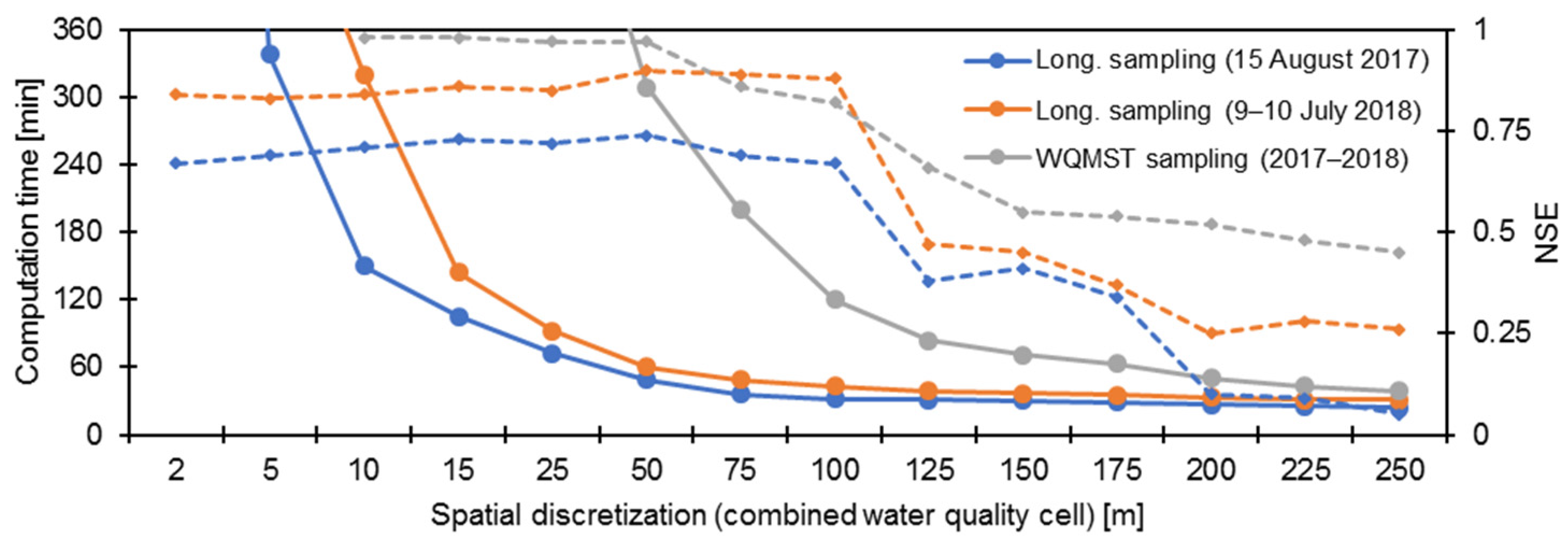
The sensitivity analysis of spatial discretization revealed that high spatial discretization (2–10 m) in model calibration setups, accompanied by computation times longer than 5-h (with an Intel Core i7-7600, 2.9 GHz processor), are not always necessary. With the purpose of maintaining a satisfactory calibration performance, it was identified that Eulerian and Lagrangian calibration strategies required combined water quality cell lengths up to 150–200 m and up to 50–100 m, respectively. An example evaluation for NO3-N with NSE values is shown in Figure 7. Acceptable NSEs, above 0.5, are obtained at spatial discretizations < 200 m for Eulerian calibration and <100 m for Lagrangian calibration. However, computation time for a single simulation could take at least 50 min using Eulerian calibration setups and at least 40 min using Lagrangian model setups.
Since Monte Carlo or GLUE methods for robust uncertainty assessment should be performed with at least 10,000 simulations [30,31] or 500–1000 simulations per parameter [64], their application is currently infeasible with the spatial discretization implemented in the calibration setups and the computer equipment used for this study. For instance, 10,000 simulations would require at least nine months with an Intel Core i7-7600, 2.9 GHz processor. For future simulations, a migration of the approach to a massive-parallel high-performance computer would be necessary to perform Monte Carlo or GLUE.
3.5. Quantification of River Denitrification Dynamics
The embedded drawback of HEC-RAS-NSM-I model about not considering denitrification during model simulations is addressed by calculating separately explicit denitrification rates (Equation (6)) and site-specific constants “a” (Equation (7)) at both studied FM river sections with weirs present and without weirs. For this purpose, boat-based measured NO3-N concentrations were used along with modelled values of flow velocity, hydraulic depth and water temperature from Section 3.1 and Section 3.2. After removing outliers of denitrification rates, according to plausible ranges (0.0–2.0 d−1) reported by [65], 1 km smoothed longitudinal profiles of denitrification rates were determined for all boat-based sampling campaigns (15 August 2017, 12 October 2017, 9–11 July 2018).
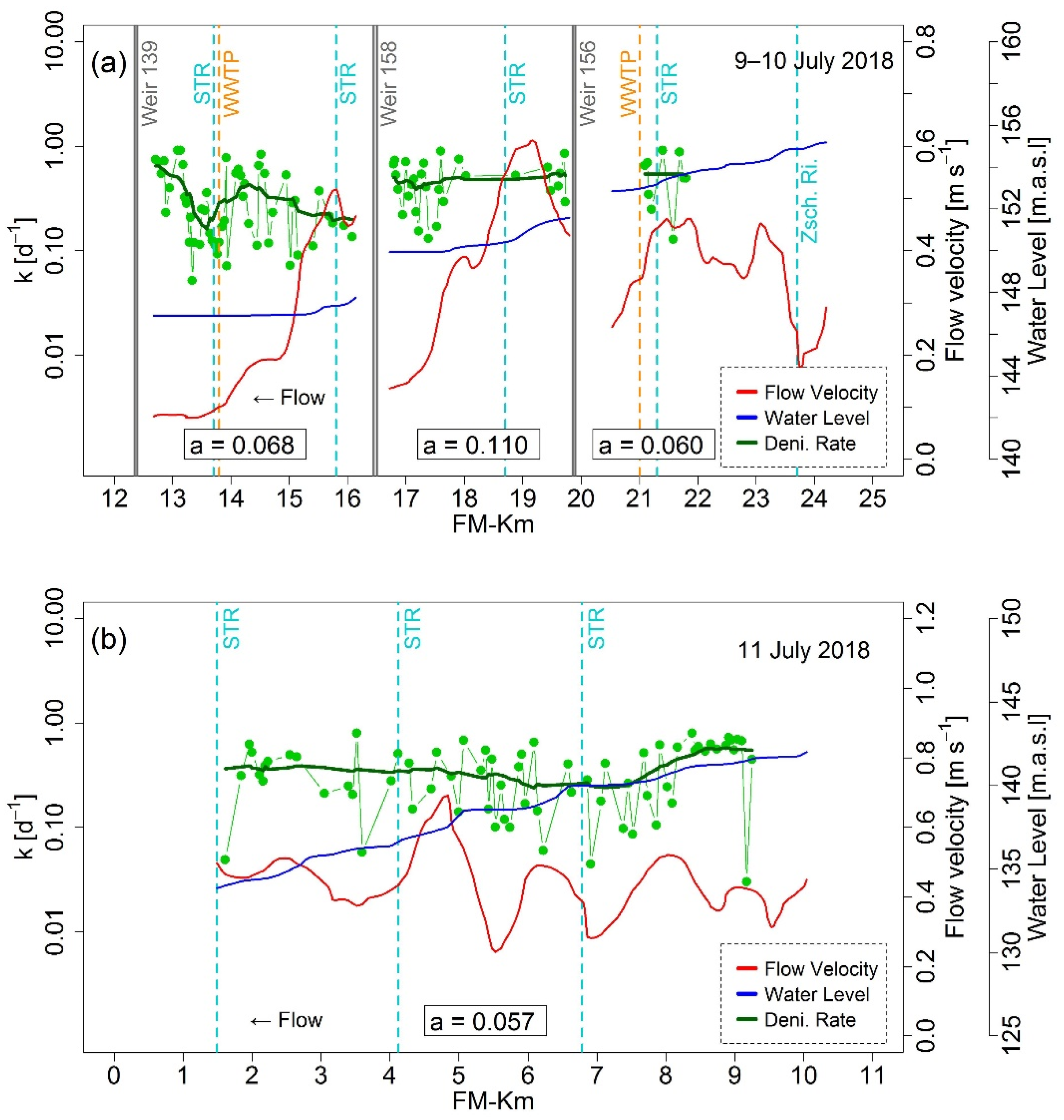
Denitrification rates for the FM river section with water retention due to weirs varied from 0.08 to 0.91 d−1 with an overall average of 0.45 d−1, while denitrification rates for the FM river section with free-flow conditions varied from 0.27 to 0.37 d−1 with an overall average of 0.32 d−1. Similarly, the computed values of the riverbed characteristic constants accounted = 0.060 in the river section from FM-km 23.5 (downstream of tributary river Zschopau) to FM-km 19.9 (Weir ID-156), = 0.110 from FM-km 19.9 (Weir ID-156) to FM-km 16.5 (Weir ID-158), = 0.068 from FM-km 16.5 (Weir ID-158) to FM-km 12.4 (Weir ID-157), and = 0.057 for the remaining downstream FM river section without weirs until the FM river mouth. In Figure 8, example longitudinal profiles of denitrification with their corresponding riverbed characteristic constants () are illustrated for the boat-based sampling campaigns between 9–11 July 2018. Denitrification was not quantified immediately downstream of Zschopau tributary river inflow because of the predominant impact of dilution and mixing on nitrate concentration. Clearly, weirs control the longitudinal river hydraulics by lowering the flow velocities from ranges of about 0.5–0.6 m s−1 to ranges of about 0.1–0.2 m s−1 and promoting constant water levels along backwater lengths of about 1.0 km (Weir ID-156), 1.5 km (Weir ID-158) and 2.0 km (Weir ID-139). Simultaneously, the tendency of accelerated denitrification rates at locations immediately upstream of weirs was again observed (Figure 8a). On the other hand, the FM river section without weirs revealed a significant variability of longitudinal flow velocity (0.24–0.69 m s−1) due to strong longitudinal changes of river cross section geometries. Additionally, an average decrease of water level slope of about 0.1% with low variability of the smoothed longitudinal denitrification profile was detected (Figure 8b).
Long-term simulations of the time period 2017–2018 quantified the nitrogen removal by denitrification for both distinctive river sections. NO3-N concentrations and loads from HEC-RAS-NSM-I model were postprocessed with the locally optimized denitrification rates. The current river condition (weirs present) was compared to a hypothetical weir removal. It is clearly perceptible that the water retention effect produced by the weirs beneficially increases NO3-N removal by denitrification (Figure 9). Along the selected 12.1 km river length, weirs contributed to reducing the mean NO3-N concentrations around two times more (by 0.29 mg L−1, 0.024 mg L−1 km−1) than in the case of their hypothetical removal (by 0.15 mg L−1, 0.012 mg L−1 km−1). Furthermore, denitrification performance varies seasonally according to existing water temperature and flow rate. During warm and low-flow periods with water temperature fluctuating around 5–27 °C, the weirs induced higher reductions of the averaged NO3-N concentrations (by 0.38 mg L−1, 0.031 mg L−1 km−1) than during cold and high-flow periods (by 0.21 mg L−1, 0.017 mg L−1 km−1) with water temperature fluctuating around 0–17 °C. Maximal reductions of NO3-N concentrations were identified during May 2017 (up to 0.73 mg L−1) and June 2018 (up to 0.97 mg L−1). Analogous results displayed the scenario of hypothetical weir removal, but in lower proportions. During warm and low-flow periods, the selected 12.1 river length with hypothetical free-flow conditions reduced slightly more averaged NO3-N concentrations (by 0.17 mg L−1, 0.014 mg L−1 km−1) than during cold and high-flow months (by 0.13 mg L−1, 0.011 mg L−1 km−1).
Overall, low-flow discharges associated with high temperature conditions allow significant nitrate removal through denitrification as previous studies reported [14,24,66]. In this study, the effect size of both conditions were also evaluated by correlating them with the corresponding reduction of NO3-N concentration. Low-flow discharges were found slightly more significant (R2 = 0.52) than high temperatures (R2 = 0.45).
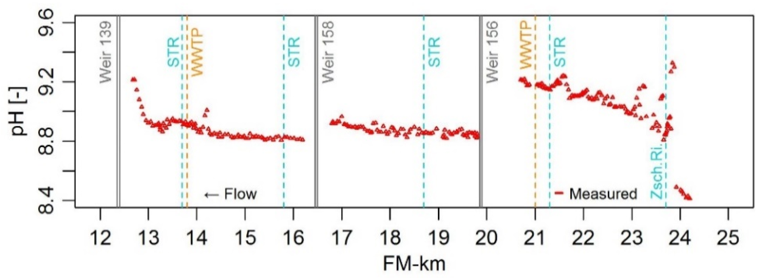
Along with photosynthesis, the presence of denitrification could also be indirectly corroborated with an increase of pH [67,68,69]. By comparing pH values at WQMST Leisnig and Erlln for the time period 2017–2018 [49], average pH values of 8.2–8.4 and 7.6–7.8 during warm and cold months were observed, respectively. Moreover, a longitudinal pH profile was developed using longitudinal measurements of pH from the boat-based sampling campaign between 9–11 July 2018 (Figure 10). An increase from pH 8.8 to pH 9.2 was observed along the flow direction within the backwater lengths produced by weirs.
In terms of quantifying the additional denitrification produced by the weirs’ influence, absolute and relative values of NO3-N loads between the scenarios “weirs present” and “weirs removed” were computed (Figure 11). As expected from the seasonal reductions of NO3-N concentrations, the highest benefit of weirs is displayed during warm and low-flow periods with mean additional N denitrified of 0.2 ton d−1 (10.9%). Furthermore, lower values of additional denitrification due to weirs were detected in summer 2017 (up to 16.9%) than in summer 2018 (up to 28.3%). The latter was drier and warmer (mean flow rate = 9.6 m3 s−1 and mean water temperature = 20.1 °C) than the former (mean flow rate = 13.7 m3 s−1 and mean water temperature = 18.4 °C). In contrast, additional N denitrified due to the weirs during cold and high-flow periods accounted for a mean of 0.04 ton d−1 (2.1%).
3.6. Methodical Limitations and Future Research
The data regression relationships and recommended stoichiometric ratios used in this study to estimate the “measured” concentrations of Org-N, NH4-N, NO2-N (for Lagrangian calibration) and algae, CBOD (for Eulerian and Lagrangian calibration) can vary according to the sampling size taken at WQMST and to the temporal fluctuations of physicochemical conditions along the FM river, such as water temperature, light and nutrient availability. With the purpose of supporting or refining such stoichiometric ratios and regression relationships, a higher temporal resolution of the measurements at WQMST and additional boat-based sampling campaigns at different seasons of the year are required.
The HEC-RAS hydrodynamic model assumes constant Manning roughness over time by omitting the temporal life cycle of aquatic vegetation life, which could impact the temporal hydraulic loads within the river water column. In addition, lateral flow rates at ungauged tributary rivers are included in HEC-RAS through a regionalized interpolation of cumulative CDA and existing water gauges along the studied FM river section. On the other hand, the coupled HEC-RAS-NSM-I model considers potential diffuse pollution from FM river subcatchments as point sources at their corresponding tributary river mouths, of which a WQMST is available for some. In the case of small tributaries without WQMST, data from WQMST of the nearest corresponding tributaries are retrieved. Despite the assumptions taken, hydraulic calibration along with Eulerian and Lagrangian calibrations of water quality constituents (e.g., N forms) were satisfactorily achieved. However, complementary water gauges and WQMST at each tributary river mouth are required to improve qualitatively the model simulations and calibrations.
The implementation of uncertainty assessment under Monte Carlo or GLUE frameworks were found impracticable, timewise, with the present available computational resources, since current HEC-RAS-NSM-I model calibration setups require very fine discretization to achieve satisfactory calibration performances. Long computation times arise mainly due to the fact that multiple calculations are performed using the explicit numerical scheme in each combined water quality cell for each parameter considered in the model. Moreover, additional time is demanded to retrieve modelled values stored in HEC-DSS output files with sizes of 0.5–1.7 GB for each simulation run. Consequently, the use of parallel processors would be necessary for in-depth uncertainty assessment.
River denitrification is spatially characterized with local first-order kinetic denitrification rates and site-specific riverbed sediment constant values () along different FM river sections. To reduce inherent uncertainties, especially at locations around weirs, direct measurement of denitrification rates is needed. This can be performed by using acetylene blockage methodology from sediment core samples [70,71] or using the N2:Ar ratio method from N2 samples [56,66].
Although the removal of weirs is the most widespread measure for river restoration, in practice, it is not a straightforward decision-making process for its implementation. The impact of weir removal may not benefit all related ecosystem services, as also discussed in [24]. While it would principally allow near-natural river connectivity, enhancing fish migration and ecological habitats, it could also lead to a higher nutrient export (e.g., N forms) to downstream river sections and the loss of some other intrinsic historic services such as recreation, fishing, navigation and flood protection. Therefore, further studies and cost evaluations for different exchanges among the ecological services is needed.
4. Conclusions
This study provides a detailed description of spatiotemporal nitrogen dynamics along the lowermost Freiberger Mulde (FM) river section within the time period 2017–2018. Multiple water quality simulations with HEC-RAS-NSM-I model together with Eulerian and Lagrangian calibrations enabled an accurate characterization of the hydraulic and water quality conditions of different FM river sections with water retention conditions due to weirs and free-flow conditions (without weirs).
The longitudinal boat-based measurements allowed better spatial identification of the nutrient entry paths as well as the refinement of N turnover rates. Namely, high ammonification was evidenced at river sections without weirs (0.015 d−1 Org-N → NH4-N) and high nitrification was evidenced at river sections with weirs present (0.17 d−1 NH4-N → NO2-N, 0.78 d−1 NO2-N → NO3-N). As the HEC-RAS-NSM-I model neglects denitrification during model simulations, it was explicitly quantified using site-specific decay rates of NO3-N concentrations based on boat-based measurements and riverbed characteristic values. Mean denitrification rates were found higher for the river sections influenced by weirs (0.45 d−1) than for the river sections with free-flow conditions (0.32 d−1). Furthermore, the outcome of long-term simulations over a 12.1 km FM river section demonstrated that the weir-influenced sections intensified denitrification by a factor of two (0.024 mg L−1 km−1) as compared to standard removal (0.012 mg L−1 km−1), with peak values detected during warm and low-flow periods. During these seasonal periods and weirs inducing around 4.5 km of backwater length (corresponding to 37% of the total distance), a mean additional N-elimination due to a denitrification of 0.2-ton d−1 (10.9%) due to weirs was determined. Since 28 weirs are located along the 124-km length of FM mainstream inducing around 25.3 km of backwater length [44], an overall mean of additional N denitrified of 1.1-ton d−1 during warm and low-flow months can be roughly estimated, without considering non-linear effects and the influence of weirs at FM tributaries.
The main drawback encountered when modelling large river sections with HEC-RAS-NSM-I and using the fine spatial discretization required for this study, is the very long computation time involved. This makes the implementation of detailed uncertainty assessment within the frameworks of Monte Carlo or GLUE methods infeasible with conventional PC equipment. Even though HEC-RAS-NSM-I model has the feature to combine water quality cells to reduce computation time, a sensitivity analysis of spatial model discretization revealed that combined water quality cells can be optimized up to 150–200 m length for Eulerian model calibration setups and up to 50–100 m length for Lagrangian model calibration setups without losing satisfactory calibration performance. However, the reduced computation times (40–50 min) for a single simulation run could still become intractable with standard computational resources for conducting a detailed uncertainty assessment.
Nevertheless, the results of this study demonstrated the significant added value of using Lagrangian data to quantify nitrogen dynamics through the refinement of N turnover rates, especially at sections upstream of weirs. Additionally, denitrification potential induced by them was found non-negligible. Hence, the implementation of such coupled Eulerian–Lagrangian calibration setups can enhance the evaluation of impacts resulting from river restoration measures, both retrospectively or prospectively, also including retardation and retention with more ecological approaches than weirs.
Author Contributions
Conceptualization, G.T.-V. and B.H.; methodology, G.T.-V.; data curation, G.T.-V.; software, G.T.-V.; validation, G.T.-V.; formal analysis, G.T.-V.; visualization, G.T.-V.; funding acquisition, B.H. and P.K.; project administration, B.H. and P.K.; writing—original draft preparation, G.T.-V.; writing—review and editing, B.H. and P.K.; supervision, B.H. and P.K. All authors have read and agreed to the published version of the manuscript.
Funding
This research was funded as part of the BOOT-Monitoring project (https://bmbf.nawam-rewam.de/en/projekt/boot-monitoring/ accessed on: 23 October 2021) by the German Federal Ministry of Education and Research (BMBF), Grant number 033W039A.
Institutional Review Board Statement
Not applicable.
Informed Consent Statement
Not applicable.
Data Availability Statement
The data is available on request from the corresponding author.
Acknowledgments
We thank the Saxon State Office for Environment, Agriculture and Geology (LfULG) for the open data policy and managers of wastewater treatment plants (WWTP) Döbeln, Westewitz and Leisnig for providing water quality data from daily operation booklets.
Conflicts of Interest
The authors declare no conflict of interest.
Appendix A
The sources of data collection for different model configurations with HEC-RAS-NSM-I using Eulerian and Lagrangian measurements are summarized in Table A1.

Table A1.
Sources of data collection for different model configurations with HEC-RAS-NSM-I.
| Parameter | Unit | Source |
|---|---|---|
| Geometry of river cross sections and weirs | - | State Dam Administration of Saxony |
| Digital terrain model | grid size 2 × 2 m | GeoSN (State Office for Geospatial Information and Surveying of Saxony) |
| Flow discharge | m3 s−1 | Water gauge network [49], WWTP operation booklets Water gauge network [49] |
| Water stage | m | |
| Global radiation | W m−2 | Climate station network [42] |
| Air temperature | °C | |
| Air humidity | % | |
| Air wind velocity | m s−1 | |
| Dissolved nitrate nitrogen (NO3-N) | mg L−1 | Water quality monitoring stations (WQMST) [49], WWTP operation booklets, Longitudinal boat-based sampling |
| Dissolved nitrite nitrogen (NO2-N) 1 | mg L−1 | |
| Dissolved ammonium nitrogen (NH4-N) 1 | mg L−1 | |
| Dissolved organic nitrogen (Org-N) 1 | mg L−1 | |
| Total organic carbon (TOC) | mg L−1 | |
| Dissolved organic carbon (DOC) | mg L−1 | |
| Dissolved oxygen (DO) | mg L−1 | |
| Water temperature | °C | |
| Phytoplankton algae (algae) 2 | mg L−1 | |
| Carbonaceous biochemical | ||
| oxygen demand (CBOD) 2 | mg L−1 | |
| pH | - |
1 Not measured with the boat-based system. Longitudinal concentrations were estimated using regressions of WQMST data. 2 Not measured. Fixed and longitudinal concentrations were estimated from stoichiometric ratios and first-order kinetics reactions.
References
- Carvalho, L.; Mackay, E.B.; Cardoso, A.C.; Baattrup-Pedersen, A.; Birk, S.; Blackstock, K.L.; Borics, G.; Borja, A.; Feld, C.K.; Ferreira, M.T.; et al. Protecting and restoring Europe’s waters: An analysis of the future development needs of the Water Framework Directive. Sci. Total Environ. 2019, 658, 1228–1238. [Google Scholar] [CrossRef] [PubMed]
- Kristensen, P.; Whalley, C.; Zal, F.N.N.; Christiansen, T. European Waters Assessment of Status and Pressures 2018; EEA Report (7/2018); European Environment Agency: Copenhagen, Denmark, 2018. Available online: https://www.eea.europa.eu/publications/state-of-water (accessed on 2 July 2021).
- Birk, S.; Bonne, W.; Borja, A.; Brucet, S.; Corral, A.; Poikane, S.; Solimini, A.; van de Bund, W.; Zampoukas, N.; Hering, D. Three hundred ways to assess Europe’s surface waters: An almost complete overview of biological methods to implement the Water Framework Directive. Ecol. Indic. 2012, 18, 31–41. [Google Scholar] [CrossRef]
- Kristensen, P.; Solheim, A.; Austnes, K. The water framework directive and state of Europe’s water. Eur. Water 2013, 44, 3–10. [Google Scholar]
- Schepers, J.S.; Varvel, G.E.; Watts, D.G. Nitrogen and water management strategies to reduce nitrate leaching under irrigated maize. J. Contam. Hydrol. 1995, 20, 227–239. [Google Scholar] [CrossRef]
- He, B.; Kanae, S.; Oki, T.; Hirabayashi, Y.; Yamashiki, Y.; Takara, K. Assessment of global nitrogen pollution in rivers using an integrated biogeochemical modeling framework. Water Res. 2011, 45, 2573–2586. [Google Scholar] [CrossRef] [PubMed]
- Gruber, N.; Galloway, J.N. An earth-system perspective of the global nitrogen cycle. Nature 2008, 451, 293–296. [Google Scholar] [CrossRef] [PubMed]
- Davis, J.R.; Koop, K. Eutrophication in Australian rivers, reservoirs and estuaries e a southern hemisphere perspective on the science and its implications. Hydrobiologia 2006, 559, 23–76. [Google Scholar] [CrossRef]
- Chapra, S.C. Surface Water-Quality Modeling; Waveland Press: Long Grove, IL, USA, 2008; pp. 419–430. [Google Scholar]
- Palmer, M.D. Water Quality Modeling: A Guide to Effective Practice; The World Bank: Washington, DC, USA, 2001; Available online: https://elibrary.worldbank.org/doi/abs/10.1596/0-8213-4863-9 (accessed on 30 June 2021).
- Grizzetti, B.; Passy, P.; Billen, G.; Bouraoui, F.; Garnier, J.; Lassaletta, L. The role of water nitrogen retention in integrated nutrient management: Assessment in a large basin using different modelling approaches. Environ. Res. Lett. 2015, 10, 065008. [Google Scholar] [CrossRef]
- Mei, K.; Zhu, Y.; Liao, L.; Dahlgren, R.; Shang, X.; Zhang, M. Optimizing water quality monitoring networks using continuous longitudinal monitoring data: A case study of Wen-Rui Tang River, China. J. Environ. Monitor. 2011, 13, 2755–2762. [Google Scholar] [CrossRef]
- Volkmar, E.C.; Dahlgren, R.A.; Stringfellow, W.T.; Henson, S.S.; Borglin, S.E.; Kendall, C.; Van Nieuwenhuyse, E.E. Using Lagrangian sampling to study water quality during downstream transport in the San Luis Drain, California, USA. Chem. Geol. 2011, 283, 68–77. [Google Scholar] [CrossRef]
- Whitehead, P.G.; Williams, R.J. A dynamic nitrogen balance model for river systems. In Proceedings of the Exeter Symposium, Exeter, UK, 19–30 July 1982; pp. 89–99. Available online: http://hydrologie.org/redbooks/a139/iahs_139_0089.pdf (accessed on 30 June 2021).
- Boyer, E.W.; Alexander, R.B.; Parton, W.J.; Li, C.; Butterbach-Bahl, K.; Donner, S.D.; Skaggs, R.W.; Grosso, S.J. Modeling denitrification in terrestrial and aquatic ecosystems at regional scales. Ecol. Appl. 2006, 16, 2123–2142. [Google Scholar] [CrossRef]
- Seitzinger, S.; Harrison, J.A.; Böhlke, J.K.; Bouwman, A.F.; Lowrance, R.; Peterson, B.; Tobias, C.; Drecht, G.V. Denitrification across landscapes and waterscapes: A synthesis. Ecol. Appl. 2006, 16, 2064–2090. [Google Scholar] [CrossRef] [Green Version]
- Brunner, G.W. HEC-RAS River Analysis System, User’s Manual, Version 5.0; U.S. Army Corps of Engineers, Institute for Water Resources, Hydrologic Engineering Center: Davis, CA, USA, 2016. Available online: https://www.hec.usace.army.mil/software/hec-ras/documentation/HEC-RAS%205.0%20Users%20Manual.pdf (accessed on 30 June 2021).
- Zhang, Z.; Johnson, B.E. Application and Evaluation of the HEC-RAS-Nutrient Simulation Module (NSM-I); U.S. Army Engineer Research and Development Center (ERDC): Vicksburg, MS, USA, 2014; Available online: https://usace.contentdm.oclc.org/digital/collection/p266001coll1/id/3855/ (accessed on 30 June 2021).
- Billen, G.; Garnier, J. Nitrogen transfers through the Seine drainage network: A budget based on the application of the Riverstrahler model. Hydrobiologia 1999, 410, 139–150. [Google Scholar] [CrossRef]
- Wagenschein, D.; Rode, M. Modelling the impact of river morphology on nitrogen retention—a case study of the Weisse Elster River (Germany). Ecol. Model. 2008, 211, 224–232. [Google Scholar] [CrossRef]
- Zhang, Z.; Johnson, B.E. Aquatic Nutrient Simulation Modules (NSMs)–Developed for Hydrologic and Hydraulic Models; U.S. Army Engineer Research and Development Center (ERDC): Vicksburg, MS, USA, 2016; Available online: https://erdc-library.erdc.dren.mil/jspui/bitstream/11681/10112/1/ERDC-EL-TR-16-1.pdf (accessed on 30 June 2021).
- Hoang, L.; van Griensven, A.; Mynett, A. Enhancing the SWAT model for simulating denitrification in riparian zones at the river basin scale. Environ. Modell. Softw. 2017, 93, 163–179. [Google Scholar] [CrossRef]
- Seitzinger, S.P.; Styles, R.V.; Boyer, E.W.; Alexander, R.B.; Billen, G.; Howarth, R.W.; Mayer, B.; Van Breemen, N. Nitrogen retention in rivers: Model development and application to watersheds in the northeastern USA. Biogeochemistry 2002, 57, 199–237. [Google Scholar] [CrossRef]
- Cisowska, I.; Hutchins, M.G. The effect of weirs on nutrient concentrations. Sci. Total Environ. 2016, 542, 997–1003. [Google Scholar] [CrossRef] [PubMed] [Green Version]
- Fehér, J.; Gáspár, J.; Szurdiné Veres, K.; Kiss, A.; Austnes, K.; Globevnik, L.; Kirn, T.; Peterlin, M.; Spiteri, C.; Prins, T.; et al. Hydromorphological Alterations and Pressures in European Rivers, Lakes, Transitional and Coastal Waters; European Topic Centre on Inland, Coastal and Marine Waters (ETC/ICM): Prague, Czech Republic, 2012; Available online: https://www.ecologic.eu/11663 (accessed on 30 June 2021).
- De Leaniz, C.G. Weir removal in salmonid streams: Implications, challenges and practicalities. Hydrobiologia 2008, 609, 83–96. [Google Scholar] [CrossRef]
- Harris, J.H.; Kingsford, R.T.; Peirson, W.; Baumgartner, L.J. Mitigating the effects of barriers to freshwater fish migrations: The Australian experience. Mar. Freshw. Res. 2017, 68, 614–628. [Google Scholar] [CrossRef]
- Caraco, N.F.; Cole, J.J. Human impact on nitrate export: An analysis using major world rivers. Ambio 1999, 28, 167–170. [Google Scholar]
- Stanley, E.H.; Doyle, M.W. A geomorphic perspective on nutrient retention following dam removal: Geomorphic models provide a means of predicting ecosystem responses to dam removal. BioScience 2002, 52, 693–701. [Google Scholar] [CrossRef] [Green Version]
- Rathod, P.; Manekar, V.L. Parameter uncertainty in HEC-RAS 1D CSU scour model. Curr. Sci. 2020, 118, 1227. [Google Scholar] [CrossRef]
- Pappenberger, F.; Beven, K.; Horritt, M.; Blazkova, S.J.J.O.H. Uncertainty in the calibration of effective roughness parameters in HEC-RAS using inundation and downstream level observations. J. Hydrol. 2005, 302, 46–69. [Google Scholar] [CrossRef]
- Greif, A. The impact of mining activities in the Ore Mountains on the Mulde river catchment upstream of the Mulde reservoir lake. Hydrol. Wasserbewirtsch. 2015, 59, 318–331. [Google Scholar]
- Spänhoff, B.; Friese, H.; Börke, P.; Kuhn, K.; Pilchowski, D.; Fischer, K. Beiträge zu den Maßnahmenprogrammen der Flussgebietseinheiten Elbe und Oder; Sächsisches Landesamt für Umwelt, Landwirtschaft und Geologie: Dresden, Germany, 2009; Available online: https://publikationen.sachsen.de/bdb/artikel/13810 (accessed on 30 June 2021).
- Küchler, L.; Harnapp, S. Gewässergütebericht 2003–Biologische Befunde der Gewässergüte Sächsischer Fließgewässer mit Gewässergütekarte; Sächsisches Landesamt für Umwelt, Landwirtschaft und Geologie: Dresden, Germany, 2003; Available online: https://publikationen.sachsen.de/bdb/artikel/13633 (accessed on 30 June 2021).
- Gebel, M.; Halbfaß, S.; Bürger, S.; Lorz, C. Long-term simulation of effects of energy crop cultivation on nitrogen leaching and surface water quality in Saxony/Germany. Reg. Environ. Change 2013, 13, 249–261. [Google Scholar] [CrossRef]
- Gebel, M.; Bürger, S.; Halbfaß, S.; Uhlig, M. Nährstoffeinträge in Sächsische Gewässer–Status quo und Ausblick bis 2027; Sächsisches Landesamt für Umwelt, Landwirtschaft und Geologie: Dresden, Germany, 2016; Available online: https://publikationen.sachsen.de/bdb/artikel/11373 (accessed on 30 June 2021).
- Klemm, W.; Greif, A.; Broekaert, J.A.C.; Siemens, V.; Junge, F.W.; van der Veen, A.; Schultze, M.; Duffek, A. A Study on Arsenic and the Heavy Metals in the Mulde River System. Acta Hydrochim. Hydrobiol. 2005, 33, 475–491. [Google Scholar] [CrossRef]
- Knittel, U.; Klemm, W.; Greif, A. Heavy metal pollution downstream of old mining camps as a result of flood events: An example from the Mulde River System, eastern part of Germany. Terr. Atmos. Ocean Sci. 2005, 16, 919–931. [Google Scholar] [CrossRef] [Green Version]
- Greif, A.; Klemm, W. Geogene Hintergrundbelastungen; Sächsisches Landesamt für Umwelt, Landwirtschaft und Geologie: Dresden, Germany, 2010; Available online: https://publikationen.sachsen.de/bdb/artikel/14924 (accessed on 30 June 2021).
- Statistisches Landesamt des Freistaates Sachsen. Bevölkerungsstand, Einwohnerzahlen, Eckdaten für Sachsen. Available online: https://www.statistik.sachsen.de/html/bevoelkerungsstand-einwohner.html (accessed on 30 June 2021).
- Sächsisches Staatsministerium für Energie, Klimaschutz, Umwelt und Landwirtschaft. Lagebericht 2016 zur Beseitigung von Kommunalem Abwasser und Klärschlamm im Freistaat Sachsen; Sächsisches Staatsministerium für Energie, Klimaschutz, Umwelt und Landwirtschaft: Dresden, Germany, 2017; Available online: https://publikationen.sachsen.de/bdb/artikel/28493 (accessed on 30 June 2021).
- Sächsisches Landesamt für Umwelt, Landwirtschaft und Geologie. Agrarmeteorologisches Messnetz Sachsen-Wetterdaten. Available online: https://www.landwirtschaft.sachsen.de/Wetter09/asp/inhalt.asp?seite=uebersicht (accessed on 30 June 2021).
- Sächsisches Landesamt für Umwelt, Landwirtschaft und Geologie. Aktuelle Wasserstände–Leisnig/Freiberger Mulde. Available online: https://www.umwelt.sachsen.de/umwelt/infosysteme/hwims/portal/web/wasserstand-pegel-566085 (accessed on 30 June 2021).
- Sächsisches Staatsministerium für Energie, Klimaschutz, Umwelt und Landwirtschaft. Querbauwerke in Sächsischen Fließgewässern. Available online: https://www.smul.sachsen.de/Wehre/Index.aspx (accessed on 30 June 2021).
- Wiek, S.; Helm, B.; Karrasch, P.; Hunger, S.; Hoffmann, T.G.; Schoenrock, S.; Klehr, W.; Six, A.; Staeglich, I.; Kuhn, K.; et al. Boat-based measurement system for longitudinal monitoring of rivers with online sensors. Hydrol. Wasserbewirtsch. 2019, 63, 19–32. [Google Scholar]
- Brunner, G.W. HEC-RAS River Analysis System, Hydraulic Reference Manual, Version 5.0; U.S. Army Corps of Engineers, Hydrologic Engineering Center: Davis, CA, USA, 2016. Available online: https://www.hec.usace.army.mil/software/hec-ras/documentation/HEC-RAS%205.0%20Reference%20Manual.pdf (accessed on 30 June 2021).
- Leonard, B.P. The ULTIMATE conservative difference scheme applied to unsteady one-dimensional advection. Comput. Methods Appl. Mech. Eng. 1991, 88, 17–74. [Google Scholar] [CrossRef]
- US Army Corps of Engineers, Institute for Water Resources, Hydrologic Engineering Center. HEC-DSSVue, HEC Data Storage System Visual Utility Engine, User’s Manual; US Army Corps of Engineers, Institute for Water Resources: Davis, CA, USA, 2009; Available online: https://www.hec.usace.army.mil/software/hec-dss/documentation/HEC-DSSVue_20_Users_Manual.pdf (accessed on 30 June 2021).
- Sächsisches Landesamt für Umwelt, Landwirtschaft und Geologie. iDA—Interdisziplinäre Daten und Auswertungen. Available online: https://www.umwelt.sachsen.de/umwelt/infosysteme/ida/index.xhtml (accessed on 30 June 2021).
- Redfield, A.C. The biological control of chemical factors in the environment. Am. Scientist 1958, 46, 230A. [Google Scholar]
- Penn, M.R.; Pauer, J.J.; Mihelcic, J.R. Biochemical oxygen demand. In Environmental and Ecological Chemistry; EOLSS Publishers: Oxford, UK, 2009; Volume 2, pp. 278–297. Available online: http://www.eolss.net/sample-chapters/c06/e6-13-04-03.pdf (accessed on 30 June 2021).
- Helm, B.; Wiek, S.; Krebs, P.; Engels, R.; Stecking, M.; Bolle, F. Die Gewässer lückenlos erfassen. Konzepte und Ansätze für eine durchgängige Aufnahme und Auswertung von Gewässereigenschaften. Korresp. Wasserwirtschaft. 2017, 10, 203–208. [Google Scholar]
- US Army Corps of Engineers, Institute for Water Resources, Hydrologic Engineering Center. Accuracy of Computed Water Surface Profiles; US Army Corps of Engineers, Institute for Water Resources: Davis, CA, USA, 1986; Available online: https://www.hec.usace.army.mil/publications/ResearchDocuments/RD-26.pdf (accessed on 30 June 2021).
- Chow, V.T. Development of Uniform Flow and Its Formulas. In Open Channel Hydraulics; McGraw-Hill Book Company: New York, NY, USA, 1959; pp. 89–127. [Google Scholar]
- Moriasi, D.N.; Arnold, J.G.; Van Liew, M.W.; Bingner, R.L.; Harmel, R.D.; Veith, T.L. Model evaluation guidelines for systematic quantification of accuracy in watershed simulations. Trans. ASABE 2007, 50, 885–900. [Google Scholar] [CrossRef]
- Ritz, S.; Dähnke, K.; Fischer, H. Open-channel measurement of denitrification in a large lowland river. Aquat. Sci. 2018, 80, 11. [Google Scholar] [CrossRef]
- Toms, I.P.; Mindenhall, M.J.; Harmann, M.M.I. Factors Affecting the Removal of Nitrate by Sediment from Rivers, Lagoons and Lakes-Technical Report TR 14; Wat. Res. Centre: Stevenage, UK, 1975. [Google Scholar]
- Alexander, R.B.; Smith, R.A.; Schwarz, G.E. Effect of stream channel size on the delivery of nitrogen to the Gulf of Mexico. Nature 2000, 403, 758–761. [Google Scholar] [CrossRef] [PubMed]
- Catalán, N.; Marcé, R.; Kothawala, D.N.; Tranvik, L.J. Organic carbon decomposition rates controlled by water retention time across inland waters. Nat. Geosci. 2016, 9, 501–504. [Google Scholar] [CrossRef]
- Cirello, J.; Rapaport, R.A.; Strom, P.F.; Matulewich, V.A.; Morris, M.L.; Goetz, S.; Finstein, M.S. The question of nitrification in the Passaic River, NJ: Analysis of historical data and experimental investigation. Water Res. 1979, 13, 525–537. [Google Scholar] [CrossRef]
- Pauer, J.J.; Auer, M.T. Nitrification in the water column and sediment of a hypereutrophic lake and adjoining river system. Water Res. 2000, 34, 1247–1254. [Google Scholar] [CrossRef]
- Deek, A.; Emeis, K.; Struck, U. Seasonal variations in nitrate isotope composition of three rivers draining into the North Sea. Biogeosciences Discuss. 2010, 7, 6051–6088. [Google Scholar]
- Dawson, R.; Murphy, K.L. The temperature dependency of biological denitrification. Water Res. 1972, 6, 71–83. [Google Scholar] [CrossRef]
- McKay, M.D.; Morrison, J.D.; Upton, S.C. Evaluating prediction uncertainty in simulation models. Comput. Phys. Commun. 1999, 117, 44–51. [Google Scholar] [CrossRef]
- Flynn, K.F.; Suplee, M.W.; Chapra, S.C.; Tao, H. Model-Based Nitrogen and Phosphorus (Nutrient) Criteria for Large Temperate Rivers: 1. Model Development and Application. J. Am. Water Resour. Assoc. 2015, 51, 421–446. [Google Scholar] [CrossRef]
- Chen, N.; Wu, J.; Chen, Z.; Lu, T.; Wang, L. Spatial-temporal variation of dissolved N2 and denitrification in an agricultural river network, southeast China. Agric. Ecosyst. Environ. 2014, 189, 1–10. [Google Scholar] [CrossRef]
- Halling-Sørensen, B.; Jorgensen, S.E. The Removal of Nitrogen Compounds from Wastewater; Elservier Science Publishers B.V: Amsterdam, The Netherlands, 1993; pp. 145–147. [Google Scholar]
- Qian, W.; Ma, B.; Li, X.; Zhang, Q.; Peng, Y. Long-term effect of pH on denitrification: High pH benefits achieving partial denitrification. Bioresour. Technol. 2019, 278, 444–449. [Google Scholar] [CrossRef] [PubMed]
- He, B.N.; He, J.T.; Wang, J.; Li, J.; Wang, F. Abnormal pH elevation in the Chaobai River, a reclaimed water intake area. Environ. Sci. Process. Impacts 2017, 19, 111–122. [Google Scholar] [CrossRef]
- Pattinson, S.N.; García-Ruiz, R.; Whitton, B.A. Spatial and seasonal variation in denitrification in the Swale–Ouse system, a river continuum. Sci. Total Environ. 1998, 210, 289–305. [Google Scholar] [CrossRef]
- Seitzinger, S.P. Denitrification in freshwater and coastal marine ecosystems: Ecological and geochemical significance. Limnol. Oceanogr. 1988, 33, 702–724. [Google Scholar] [CrossRef]
Figure 1.
Study area of FM river catchment and location of existing weirs, water gauges, water quality monitoring stations (WQMST) and wastewater treatment plants (WWTP) along the FM main river. Dark blue line: the 26.9 km river section.
Figure 1.
Study area of FM river catchment and location of existing weirs, water gauges, water quality monitoring stations (WQMST) and wastewater treatment plants (WWTP) along the FM main river. Dark blue line: the 26.9 km river section.

Figure 2.
Regressions of N forms using fixed measurements at WQMST along FM river.

Figure 3.
Calibration of flow rate hydrographs at water gauges Mahlitzsch (A) and Leisnig (B).

Figure 4.
Calibrated time series of (a) water temperature, (b) DO, (c) CBOD, (d) algae, (e) Org-N, (f) NH4-N, (g) NO2-N and (h) NO3-N at WQMST Leisnig (FM-km 11.9). LOD: limit of detection.
Figure 4.
Calibrated time series of (a) water temperature, (b) DO, (c) CBOD, (d) algae, (e) Org-N, (f) NH4-N, (g) NO2-N and (h) NO3-N at WQMST Leisnig (FM-km 11.9). LOD: limit of detection.


Figure 5.
Calibrated time series of (a) water temperature, (b) DO, (c) CBOD, (d) algae, (e) Org-N, (f) NH4-N, (g) NO2-N and (h) NO3-N at WQMST Erlln (FM-km 0.4). LOD: limit of detection.
Figure 5.
Calibrated time series of (a) water temperature, (b) DO, (c) CBOD, (d) algae, (e) Org-N, (f) NH4-N, (g) NO2-N and (h) NO3-N at WQMST Erlln (FM-km 0.4). LOD: limit of detection.


Figure 6.
Longitudinal profiles of measured and modelled NO3-N concentrations along FM river section (a) with weirs present and (b) without weirs, based on boat-based sampling campaigns on 15 August 2017, 9–10 July 2018, 12 October 2017 and 11 July 2018. WWTP = wastewater treatment plant; STR = small tributary river; Zsch. Ri. = Zschopau River.

Figure 7.
Computation time (solid lines) and calibration performance using NSE values (dashed lines) for NO3-N with different spatial discretization (combined water quality cell).
Figure 7.
Computation time (solid lines) and calibration performance using NSE values (dashed lines) for NO3-N with different spatial discretization (combined water quality cell).

Figure 8.
Longitudinal profiles of denitrification rate, flow velocity and water level for FM river section (a) with weirs present and (b) without weirs, based on modeled hydraulic variables and boat-based measurements on 9–11 July 2018. WWTP = wastewater treatment plant; STR = small tributary river; Zsch. Ri. = Zschopau River; a = site-specific riverbed constant.

Figure 9.
Time series plots for the time period 2017–2018 under scenarios of “weirs present” and “weirs removed” showing comparatively (a) the NO3-N concentration between FM-km 23.5 and FM-km 11.4 along with flow rate and water temperature and (b) the corresponding reduction of NO3-N concentration due to denitrification. XS = river cross section.

Figure 10.
Longitudinal profile of measured pH concentrations along FM river section with weirs present based on boat-based sampling campaigns between 9–10 July 2018. WWTP = wastewater treatment plant; STR = small tributary river; Zsch. Ri. = Zschopau River.
Figure 10.
Longitudinal profile of measured pH concentrations along FM river section with weirs present based on boat-based sampling campaigns between 9–10 July 2018. WWTP = wastewater treatment plant; STR = small tributary river; Zsch. Ri. = Zschopau River.

Figure 11.
Absolute and relative quantification of additional N denitrified due to weirs between FM-km 23.5 and FM-km 11.4 for the time period 2017–2018.
Figure 11.
Absolute and relative quantification of additional N denitrified due to weirs between FM-km 23.5 and FM-km 11.4 for the time period 2017–2018.

Table 1.
Calibrated turnover rates using HEC-RAS-NSM-I model with Eulerian data (WQMST).
| Turnover Rate | WQMST Leisnig (FM-km 11.9, Weirs Present) | WQMST Erlln (FM-km 0.4, without Weirs) |
|---|---|---|
| Sediment oxygen demand (d−1) | 0.20 | 0.20 |
| Atmospheric reaeration (d−1) | 0.50 | 0.50 |
| Algal photosynthesis (mg O mg Algae−1) | 1.80 | 1.80 |
| Algal respiration (mg O mg Algae−1) | 1.70 | 1.70 |
| CBOD oxidation (d−1) | 0.02 | 0.02 |
| CBOD settling (d−1) | 0.00 | 0.00 |
| Nitrification inhibition Factor (KNR) (mg L−1) | 0.65 | 0.65 |
| Maximum algal growth rate (d−1) | 1.00 | 1.00 |
| Algal settling rate (m d−1) | 0.10 | 0.10 |
| Algae → Org-N (mg N mg Algae−1) | 0.09 | 0.09 |
| Org-N settling (d−1) | 0.001 | 0.001 |
| Org-N → NH4-N (d−1) | 0.003 | 0.010 |
| NH4-N → NO2-N (d−1) | 0.29 | 0.15 |
| NO2-N → NO3-N (d−1) | 0.71 | 0.55 |
Table 2.
Model performance using HEC-RAS-NSM-I at WQMST Leisnig and Erlln.
| Parameter | WQMST Leisnig (FM-km 11.9) | WQMST Erlln (FM-km 0.4) | ||||||
|---|---|---|---|---|---|---|---|---|
| RMSE | RSR | NSE | PBIAS % | RMSE | RSR | NSE | PBIAS % | |
| Water temperature | 0.967 | 0.132 | 0.982 | −0.4 | 1.482 | 0.189 | 0.963 | 2.5 |
| DO | 0.643 | 0.371 | 0.858 | −1.4 | 1.012 | 0.686 | 0.515 | −3.0 |
| CBOD | 0.129 | 0.475 | 0.766 | −1.0 | 0.166 | 0.593 | 0.638 | −6.5 |
| Algae | 1.490 | 0.609 | 0.617 | −14.2 | 1.985 | 0.600 | 0.630 | −19.7 |
| Org-N | 0.261 | 0.810 | 0.321 | −18.3 | 0.249 | 0.664 | 0.547 | −16.4 |
| NH4-N 1 | 0.020 | 0.718 | 0.448 | −3.6 | 0.019 | 0.646 | 0.553 | 3.6 |
| NO2-N 1 | 0.005 | 0.695 | 0.497 | −15.1 | 0.005 | 0.722 | 0.458 | −13.2 |
| NO3-N | 0.179 | 0.113 | 0.987 | −1.7 | 0.270 | 0.158 | 0.974 | −2.3 |
1 Measurement values less than LOD were removed for the calculation of goodness-of-fit indices.
Table 3.
Calibrated turnover rates using HEC-RAS-NSM-I model with boat-based data.
| Turnover Rate | Boat-Based Data (FM River Section with Weirs Present) | Boat-Based Data (FM River Section without Weirs) |
|---|---|---|
| Algae → Org-N (mg-N mg-Algae−1) | 0.09 | 0.09 |
| Org-N Settling (d−1) | 0.005 | 0.005 |
| Org-N → NH4-N (d−1) | 0.003 | 0.015 |
| NH4-N → NO2-N (d−1) | 0.17 | 0.13 |
| NO2-N → NO3-N (d−1) | 0.78 | 0.52 |
Table 4.
Model performance using HEC-RAS-NSM-I with boat-based data.
| Parameter | FM River Section with Weirs | FM River Section without Weirs 1 | |||
|---|---|---|---|---|---|
| RMSE | PBIAS % | NSE | RMSE | PBIAS % | |
| Algae | (0.261, 0.574) | (−1.0, 2.4) | (0.60, 0.77) | (0.135, 0.722) | (1.2, 1.7) |
| Org-N | (0.010, 0.013) | (0.1, 0.7) | (0.61, 0.71) | (0.001, 0.002) | (0.1, 0.1) |
| NH4-N | (0.001, 0.001) | (−0.2, 0.1) | (0.52, 0.80) | (0.001, 0.001) | (0.1, 0.2) |
| NO2-N | (0.001, 0.001) | (0.1, 0.3) | (0.71, 0.78) | (0.001, 0.002) | (−0.9, 0.1) |
| NO3-N | (0.086, 0.092) | (−0.3, 0.3) | (0.67, 0.89) | (0.018, 0.380) | (−0.2, −1.6) |
1 NSE not calculated because measured data and derived data from regressions presented very low spatial variability.
Publisher’s Note: MDPI stays neutral with regard to jurisdictional claims in published maps and institutional affiliations. |
© 2022 by the authors. Licensee MDPI, Basel, Switzerland. This article is an open access article distributed under the terms and conditions of the Creative Commons Attribution (CC BY) license (https://creativecommons.org/licenses/by/4.0/).
Share and Cite
MDPI and ACS Style
Teran-Velasquez, G.; Helm, B.; Krebs, P. Longitudinal River Monitoring and Modelling Substantiate the Impact of Weirs on Nitrogen Dynamics. Water 2022, 14, 189. https://doi.org/10.3390/w14020189
AMA Style
Teran-Velasquez G, Helm B, Krebs P. Longitudinal River Monitoring and Modelling Substantiate the Impact of Weirs on Nitrogen Dynamics. Water. 2022; 14(2):189. https://doi.org/10.3390/w14020189
Chicago/Turabian StyleTeran-Velasquez, Geovanni, Björn Helm, and Peter Krebs. 2022. "Longitudinal River Monitoring and Modelling Substantiate the Impact of Weirs on Nitrogen Dynamics" Water 14, no. 2: 189. https://doi.org/10.3390/w14020189
Note that from the first issue of 2016, this journal uses article numbers instead of page numbers. See further details here.