
Investigation of Hyperparameter Setting of a Long Short-Term Memory Model Applied for Imputation of Missing Discharge Data of the Daihachiga River


1
Graduate School of Civil Engineering, Gifu University, Gifu 501-1193, Japan
2
River Basin Research Center, Gifu University, Gifu 501-1193, Japan
*
Authors to whom correspondence should be addressed.
Water 2022, 14(2), 213; https://doi.org/10.3390/w14020213
Submission received: 24 November 2021
/
Revised: 6 January 2022
/
Accepted: 6 January 2022
/
Published: 12 January 2022
(This article belongs to the Special Issue Hydrological Modelling and Hydrometeorological Extreme Prediction)
Abstract
:Missing observational data pose an unavoidable problem in the hydrological field. Deep learning technology has recently been developing rapidly, and has started to be applied in the hydrological field. Being one of the network architectures used in deep learning, Long Short-Term Memory (LSTM) has been applied largely in related research, such as flood forecasting and discharge prediction, and the performance of an LSTM model has been compared with other deep learning models. Although the tuning of hyperparameters, which influences the performance of an LSTM model, is necessary, no sufficient knowledge has been obtained. In this study, we tuned the hyperparameters of an LSTM model to investigate the influence on the model performance, and tried to obtain a more suitable hyperparameter combination for the imputation of missing discharge data of the Daihachiga River. A traditional method, linear regression with an accuracy of 0.903 in Nash–Sutcliffe Efficiency (NSE), was chosen as the comparison target of the accuracy. The results of most of the trainings that used the discharge data of both neighboring and estimation points had better accuracy than the regression. Imputation of 7 days of the missing period had a minimum value of 0.904 in NSE, and 1 day of the missing period had a lower quartile of 0.922 in NSE. Dropout value indicated a negative correlation with the accuracy. Setting dropout as 0 had the best accuracy, 0.917 in the lower quartile of NSE. When the missing period was 1 day and the number of hidden layers were more than 100, all the compared results had an accuracy of 0.907–0.959 in NSE. Consequently, the case, which used discharge data with backtracked time considering the missing period of 1 day and 7 days and discharge data of adjacent points as input data, indicated better accuracy than other input data combinations. Moreover, the following information is obtained for this LSTM model: 100 hidden layers are better, and dropout and recurrent dropout levels equaling 0 are also better. The obtained optimal combination of hyperparameters exceeded the accuracy of the traditional method of regression analysis.
1. Introduction
Missing observational data pose an unavoidable problem in the hydrological field. It can be caused by various factors, such as malfunction of the observation device, errors in manual data input, limitations of the measuring equipment, etc. The missing data will reduce the efficiency of relevant hydrological research, and lead to further problems in decision-making in hydrological management [1]. Up to the present, the missing data have been complemented successfully by traditional methods, such as the tank and runoff models [2,3], and regression analysis using data from neighboring observation points. However, these traditional methods have limitations in the cost of time and manpower and peak time shift.
Deep learning technology has recently been developing rapidly, and has started to be applied in the hydrological field. Being one of the network architectures used in deep learning, Long Short-Term Memory (LSTM) was applied largely in related research, such as flood forecasting [4,5,6,7,8] and discharge prediction [9,10,11,12], and the performance of the LSTM model was compared with other deep learning models on the application of runoff estimations. Hu et al. [8] applied an Artificial Neural Network (ANN) and LSTM on the simulation of a rainfall-runoff process. Xiang et al. [9] conducted an application of LSTM on an estimation of hourly rainfall-runoff, and compared the performance with traditional models. Lee et al. [12] performed runoff simulations of a river by LSTM and a physics-based model. Bai et al. [13] compared the robustness of two hydrologic models with an LSTM model in a prediction of runoff. Fan et al. [14] compared the performance of an LSTM model with ANN and the Soil and Water Assessment Tool (SWAT) on runoff modelling of a river basin. All the studies mentioned above pointed out that the LSTM model had better performance or was more stable than the compared models in the application of runoff estimations. Additionally, the potential of LSTM in the forecasting of evapotranspiration was also explored, and the fact was known that the performance of the model can be affected by different factors. Granata and Di Nunno [15] deployed LSTM and a nonlinear autoregressive network with exogenous inputs (NARX) for the prediction of evapotranspiration. The results indicated that each model has its own advantages in different climatic conditions, since the model performance can be affected by local climatic conditions significantly. Chen et al. [16] compared the performance of LSTM with several other models in an estimation of daily reference evapotranspiration. The model performance was influenced by the type of available features. Ferreira and da Cunha [17] investigated the potential of deep learning models, machine learning models, and a combined model in the forecasting of daily reference evapotranspiration in local and regional scenarios. Even if the model performance varied with different input data combinations, the combined model, which consisted of LSTM and a convolutional neural network (CNN), had the best accuracy in both local and regional scenarios.
However, the tuning of hyperparameters influences the performance of an LSTM model. Exploring optimal hyperparameters for an LSTM model is already a study objective in applications of LSTM models in fields other than hydrology, such as sequence labeling [18], network attack detection [19], stock market prediction [20], highway traffic prediction [21], etc. In the case of hydrology, the tuning of hyperparameters is a necessary step before the application of the model in other research [4,5,22,23,24,25]; however, no sufficient knowledge has been obtained.
In our previous study [26], we investigated the feasibility of missing discharge data imputation of the Daihachiga River by an LSTM model. The LSTM model was proved to be feasible, and had better performance than linear regression analysis, even though the hyperparameter was not tuned. In this study, we tuned the hyperparameters of an LSTM model to investigate the influence on the model performance, and tried to obtain a more suitable hyperparameter combination in the imputation of missing data using an LSTM model. A suitable hyperparameter combination of LSTM will improve the performance of the model on missing discharge data imputation, and it will have reference value in hydrological research.
2. Materials and Methods
2.1. Study Area
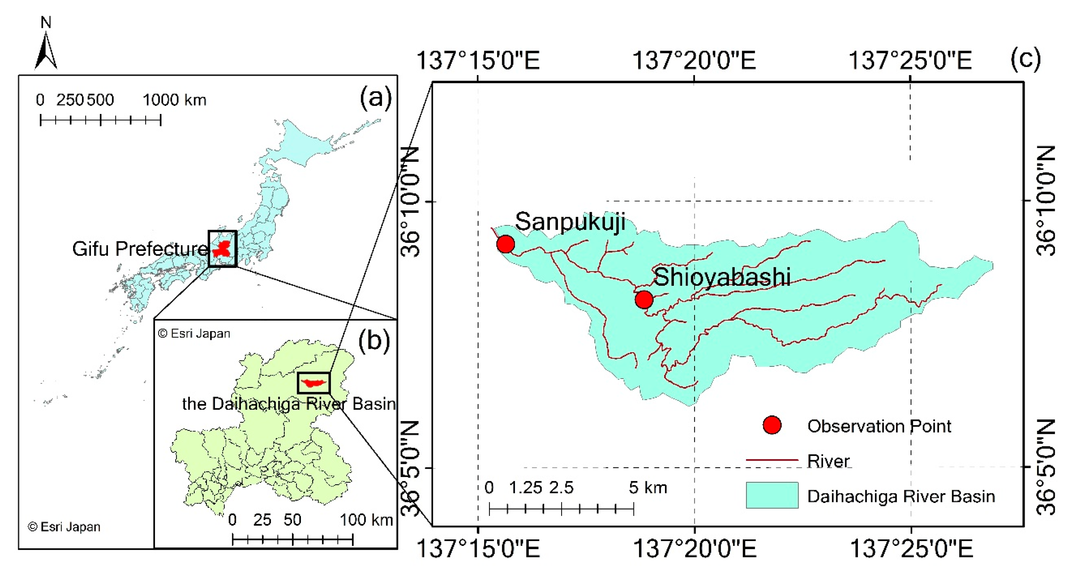
The study area of the present work is the Daihachiga River Basin (Figure 1). The Daihachiga River belongs to the Jinzu River system. It starts from Hikagedaira Mountain, which is located in the east of Takayama City, Gifu Prefecture, Japan. The river flows from the east to the west, and merges into the Miya River in the urban area of Takayama. The river basin has about 1800 mm of mean annual precipitation, 10.9 °C of mean annual air temperature, and 60.4 km2 of catchment area [27,28].
2.2. Data
Discharge data of the Daihachiga River were used in this study. The data were observed at one-hour intervals by the Gifu Prefecture at the observation points of Shioyabashi (36°8′8″ N, 137°18′50″ E, 617 m) and Sanpukuji (36°9′12″ N, 137°15′38″ E, 563 m) (Figure 1). The data of 2008 and 2009 were used as training and validation data, respectively. In addition, precipitation and air temperature data at one-hour intervals observed by the Japan Meteorological Agency in 2008 and 2009, Takayama (36°09′18″ N, 137°15′11″ E, 561 m), were used during the training of the discharge data.
2.3. Method
2.3.1. LSTM Model
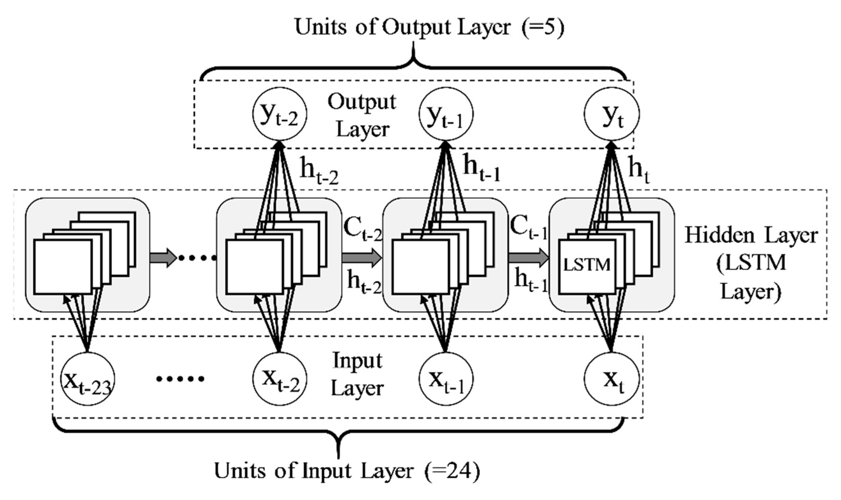
The structure of the LSTM model used in this study is shown in Figure 2. At the time step t in LSTM, cell state Ct and hidden state ht, which is the output from the LSTM unit, are passed to the LSTM of the next time step t + 1. In an LSTM unit, ht can be obtained from ht−1, Ct−1 and xt, which is the input value at time step t. In an output unit, output yt from the output layer can be obtained from the output of LSTM, ht. The procedure is the same as the standard RNN model. In the case of LSTM, xt, ht−1 and Ct−1 will be passed through the input gate, output gate, and forget gate in the LSTM unit, and the vanishing gradient problem can be solved [29,30]. The units of the input layer and output layer of the LSTM used in this study are 24 and 5, respectively (Figure 2). The other hyperparameters set for training are shown below:
- : number and type of input variables.
- : backtracked time steps of data used for the training.
- : number of units of hidden layer.
- : dropout.
- : recurrent dropout.
The purpose of this study is to impute the missing values. Therefore, it is possible to use past or future data of the observation point for which the missing value must be estimated as input values. Because LSTM is a structure that propagates information from the past to the future, future information is not as effective as present information as input data. Therefore, in this study, the past data Backts steps before will be used as training data. When the data to be estimated are used as input data for training, considering the existence of missing data, the data from t-Backts to t-Backts-24 are used to estimate the data at time t. This means that if there is a Backts steps gap of missing data, this part can be estimated by the data before the gap. Thus, the hyperparameter Backts only has a value when the estimated data were also used as input data. For other input data than the estimated point, such as temperature and precipitation, data from time t to t-24 are used to estimate time t.
The LSTM was actualized by Python 3.7.4 with the Keras 2.3.1 and NumPy 1.18.1 libraries. The activation function was an exponential linear unit (ELU), and the optimizer was Adam.
2.3.2. Hyperparameter Settings and Data Training
LSTM training was carried out by 90 kinds of hyperparameter combination (Table S1) settings to figure out the best one. The discharge data of the Daihachiga River, and the air temperature and precipitation data of Takayama were used as input variables. Several specified values were assigned for each hyperparameter in the training (Table 1). Backts = 24 and 168 assume the missing period of 1 day and 7 days, respectively. In each training period, values of dropout and recurrent dropout were assigned identically. The hyperparameter values were assigned by trial-and-error approach in those 90 trainings. The estimated data were the discharge of Shioyabashi. Table 2 shows the input variable types for each case. For example, in the setting of Backts = 24, Case 1 takes as input data two variables: the discharge data from t-Backts to t-Backts-24 at the Shioyabashi, and the precipitation at t to t-24. Case 2 takes as input data two variables: the discharge data from t-Backts to t-Backts-24 at the Shioyabashi, and the discharge data from t to t-24 at Sanpukuji. Case 5 takes one variable as input data: the discharge data from t-Backts to t-Backts-24 at the Shioyabashi. Additionally, Case 9 takes as input data one variable: the discharge data from t to t-24 at the Sanpukuji.
The evaluation method of Kojima et al. [26] was referenced and improved advisably in this study. Because the result of each training of Stochastic Gradient Decent (SGD) is different, which means the accuracy of each training is different, the ensemble average of multiple training results was calculated to cancel such differences. For each combination of hyperparameters, the training was repeated 500 times. From the results of 500 trainings, N ensemble members of them were picked out randomly, and the ensemble average was calculated. The Nash–Sutcliffe model efficiency coefficients (NSE) [31] of these average values were calculated for the evaluation. NSE is a coefficient to evaluate the estimation results of a hydrological model. Additionally, the evaluation metrics commonly used on deep learning, such as Root Mean Squared Error (RMSE) and Mean Absolute Error (MAE), were regarded as the potential options to evaluate the model accuracy of this study. The N varies from 1 to 50, and for each N, the random pick out was carried out 40 times. The average and standard deviation of NSE of these 40 ensemble average values were calculated, and the variation of 5th percentile (P5) on N = 1–50 was evaluated. Even if the result was dispersed, P5 can indicate that 95% of the results were better than it.
2.3.3. Traditional Method
The linear regression equation was used as the traditional imputation method compared with the new method using deep learning, which was proposed in this study. When is the discharge data observed on Shioyabashi at time , and is the discharge data observed on Sanpukuji at time , the linear regression model is defined as follows Equation (1):
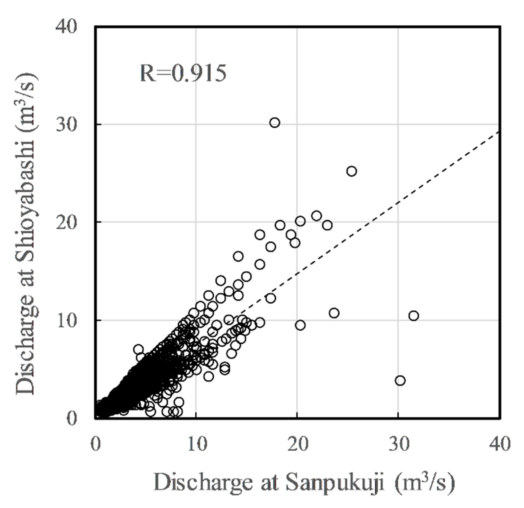
where and are the regression parameters. and were estimated with the data of 2008, as shown in Figure 3. The x axis is the discharge data at Sanpukuji (), and the y axis is the discharge data at Shioyabashi (), where the correlation coefficient R was 0.915. The dotted line is the linear regression model. The accuracy, which was evaluated with the discharge data in 2009, was 0.903 in NSE.
A tank model optimized by the Shuffled Complex Evolution (SCE-UA) method was also considered as the comparison target of the deep learning. In this model, the precipitation of Takayama in 2009 was used as input, and the discharge height was estimated. The equation of the model is shown as follows Equation (2):
where Q is the discharge height (mm/h), R is the precipitation, and E is the evaporation. The discharge coefficient was set as 0.9. The evaporation was set as 0, since it was complicated and hard to grasp the exact amount of evaporation in this case. However, the R of the tank model was 0.888 (Figure 4), and the NSE was 0.771, which is lower than the linear regression model. The aim of this study is to propose a new method to obtain an improved accuracy. Thus, the higher accuracy of the linear regression model was chosen as the goal to be exceeded by the new method.
3. Results and Discussion
3.1. Evaluation Metrics
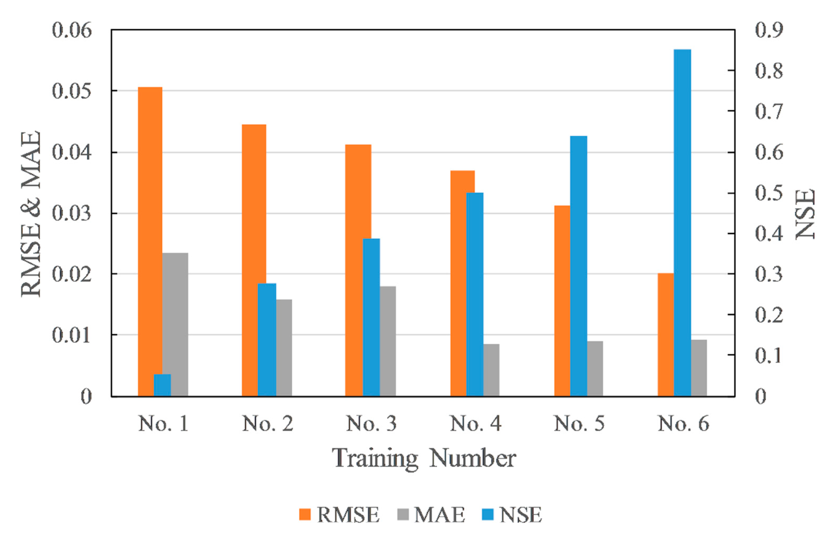
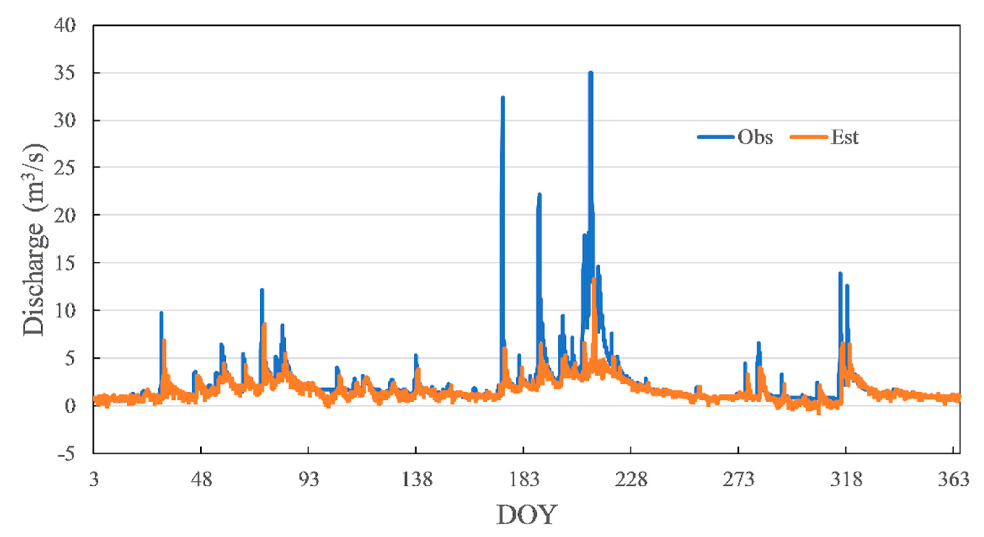
NSE, RMSE, and MAE were tested on several random trainings. The results indicated a basically stable relationship between these metrics (Figure 5). The NSE has a negative correlation with RMSE. The trend of MAE was expected to be the same as RMSE. However, it is different between Training No. 2 and Training No. 3. Even if Training No. 2 has a higher RMSE and lower NSE than Training No. 3, its MAE was lower. The hydrographs of Training No. 2 and Training No. 3 are shown in Figure 6 and Figure 7, respectively. The blue line is observed data, and the orange line is estimated data. The line of estimated data overlaps the line of observed data more in Training No. 2, which has led to a result of a lower MAE value than Training No. 3. On the other hand, Training No. 3 was able to estimate peak discharge more accurately than Training No. 2, which made the RMSE of No. 3 lower than Training No. 2. However, these results were compared under a condition that NSE is under 0.4, which cannot be regarded as acceptable model accuracy. Since NSE can reflect the trend of RMSE and MAE, and was frequently used in recent studies, it was chosen as the evaluation metric of this study.
3.2. Number of Members for Ensemble Average
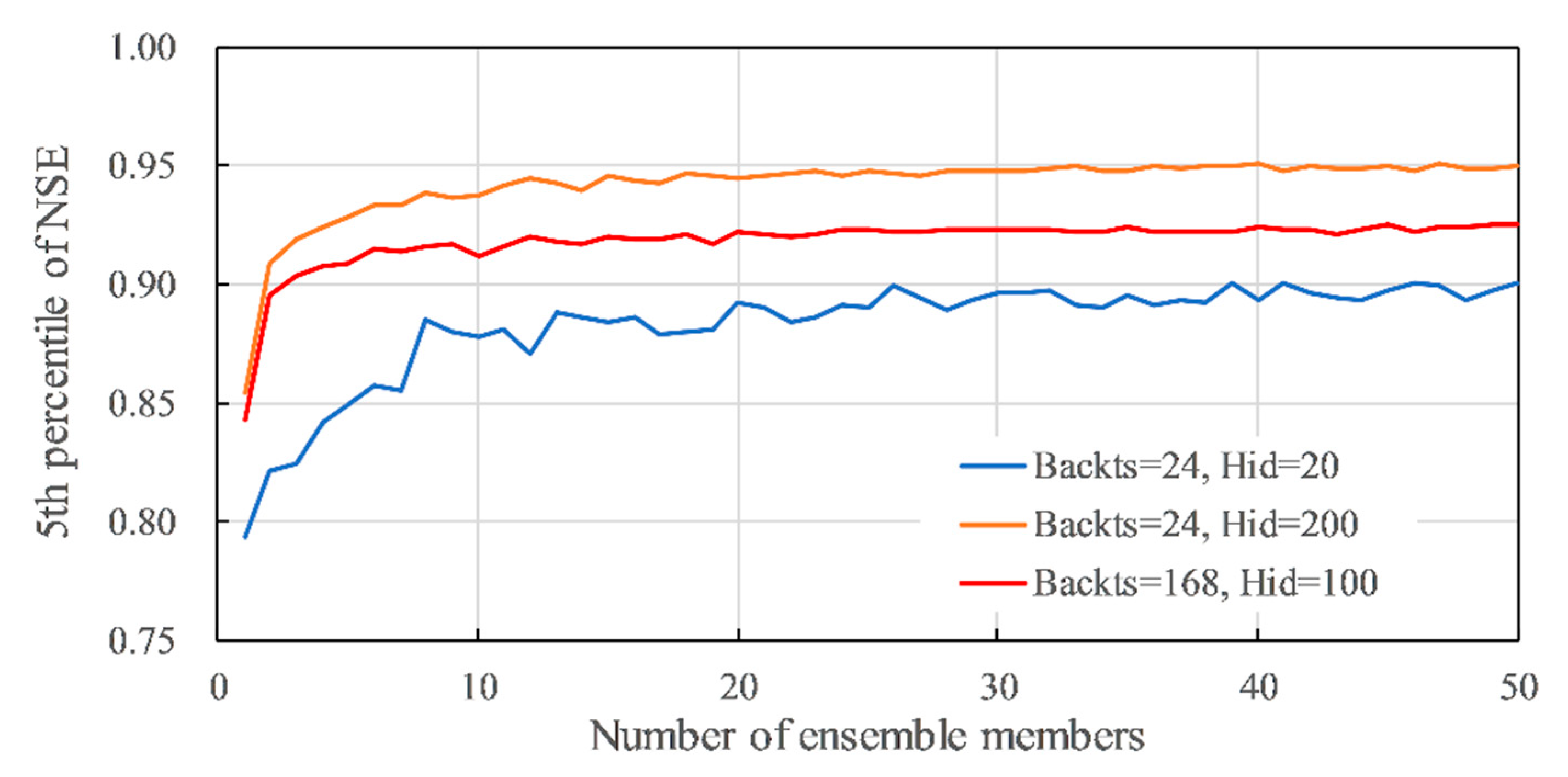
The P5 of the NSE from the number of ensemble members N = 1 to 50 for Case 2 is shown in Figure 8 as an example. The blue line shows the results with Backts = 24, Hid = 20, the orange line shows the results with Backts = 24, Hid = 200, and the red line shows the results with Backts = 168, Hid = 100. At the blue line, where the number of hidden layers (Hid) is small, the accuracy is generally low, and the P5 of NSE = 0.90 is the best. For the orange and red lines, where Hid > 100, increasing the number of ensemble members results in an accuracy of NSE > 0.92, which is greater than the 0.903 reference accuracy. In brief, the variation curves of P5 of NSE become flat, and keep the accuracy level when N ≤ 20. Thus, in this study, the training results were evaluated by the P5 of NSE for N = 30 for safety to avoid the dispersion of different training results.
3.3. Type of Input Variables
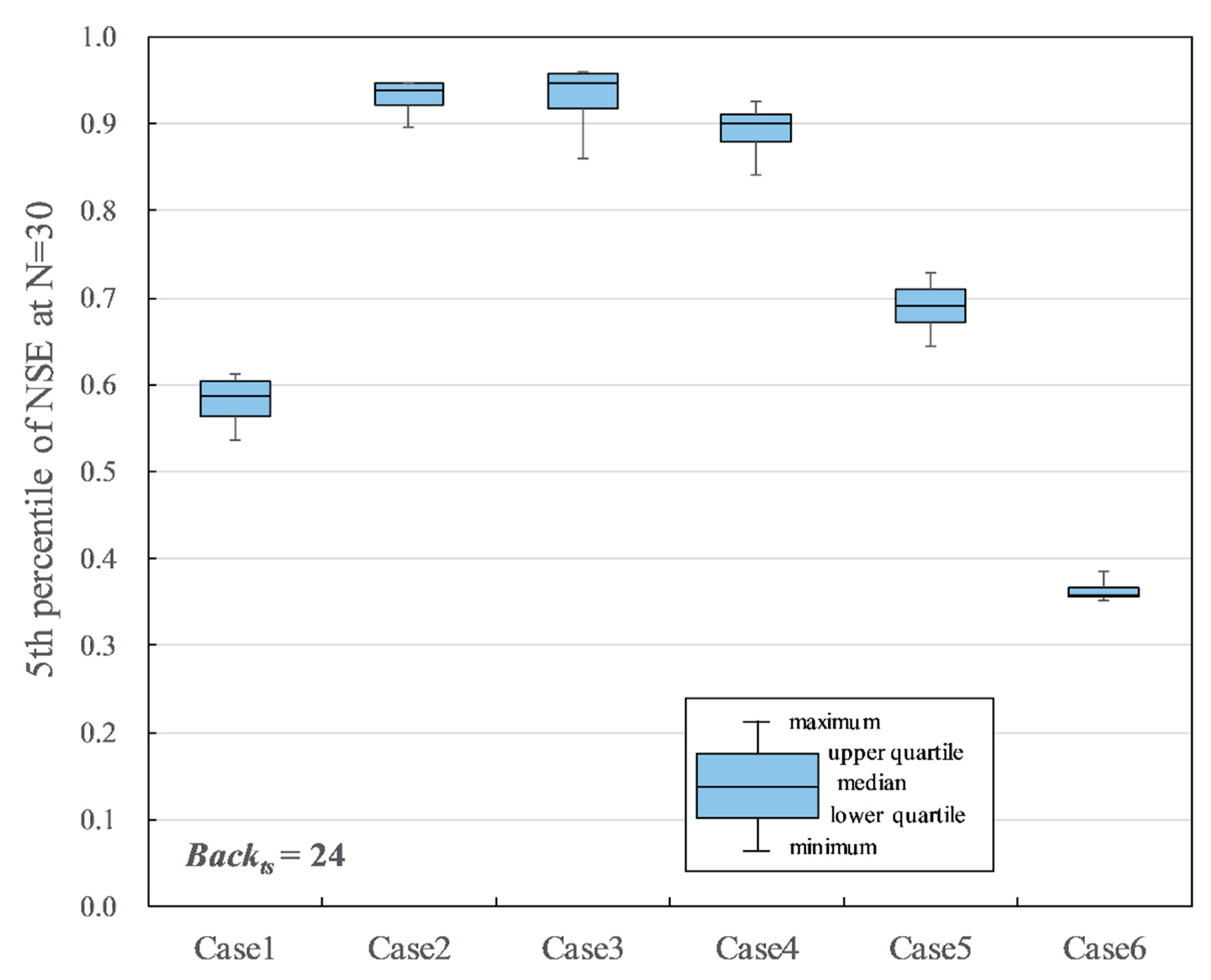
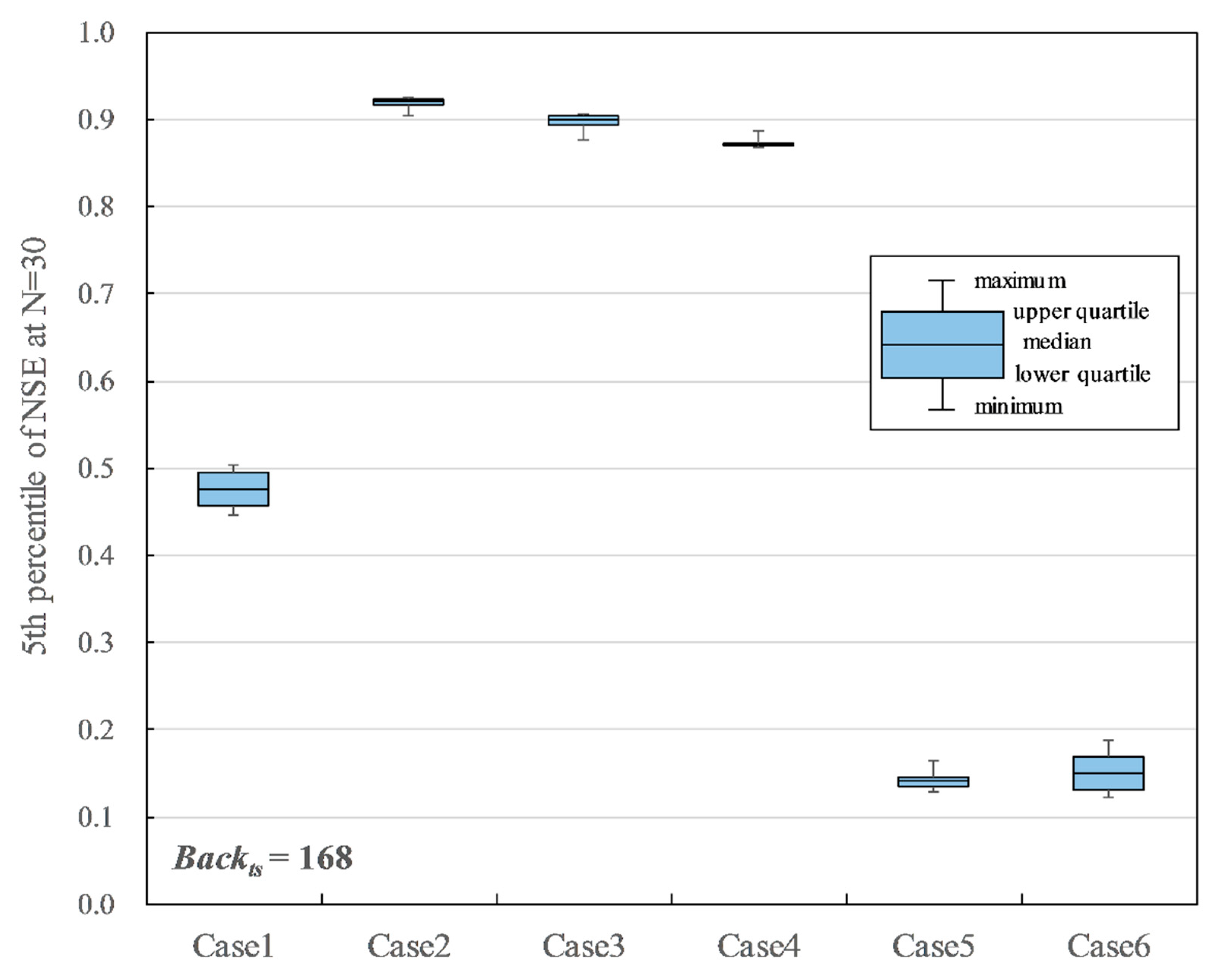
The P5 of NSE, when N = 30, was compared to evaluate the influence of each training hyperparameter to the result. There are four kinds of Hid combinations for each input variable case. Figure 9, Figure 10 and Figure 11 show the four combinations of the hyperparameter settings summaries of the results with Drp = 0 and Drpr = 0. Figure 9 and Figure 10 show the results of Case 1–6 with Backts = 24, which assumed a 1-day missing period, and Backts = 168, which assumed a 7-day missing period, respectively. In Figure 9, Case 2, Case 3, and Case 4, which used the discharge data of both Shioyabashi and Sanpukuji as input data, were relatively good. Case 2 and Case 3 indicate 0.939 and 0.947 in the median of P5 of NSE, respectively. They are over the reference accuracy 0.903, which is the accuracy of the linear regression model. Case 4, which used air temperature as one of the input data factors, indicates 0.900 in the median of P5 of NSE, which was slightly less than the reference accuracy. The lower quartiles for Case 2 and Case 3 were 0.922 and 0.917, respectively, which were better than the reference accuracy. However, the minimum for Case 2 and Case 3 were 0.896 and 0.860, respectively, which were slightly less than the reference accuracy. It must be noted that Case 3, which used precipitation as one of the input data factors, has a wide variation in accuracy depending on different hyperparameter settings. In Figure 10, Case 2, Case 3, and Case 4 have relatively good accuracy, as is seen in Figure 9. Case 2 indicates 0.922 in the median of P5 of NSE, which is over the reference accuracy. However, the median of Case 3 and Case 4 are 0.899 and 0.871, respectively, which are less than the reference accuracy. The minimum for Case 2 is 0.904, which is over the reference accuracy. Thus, Case 2 is appropriate for the input data when Backts = 168.
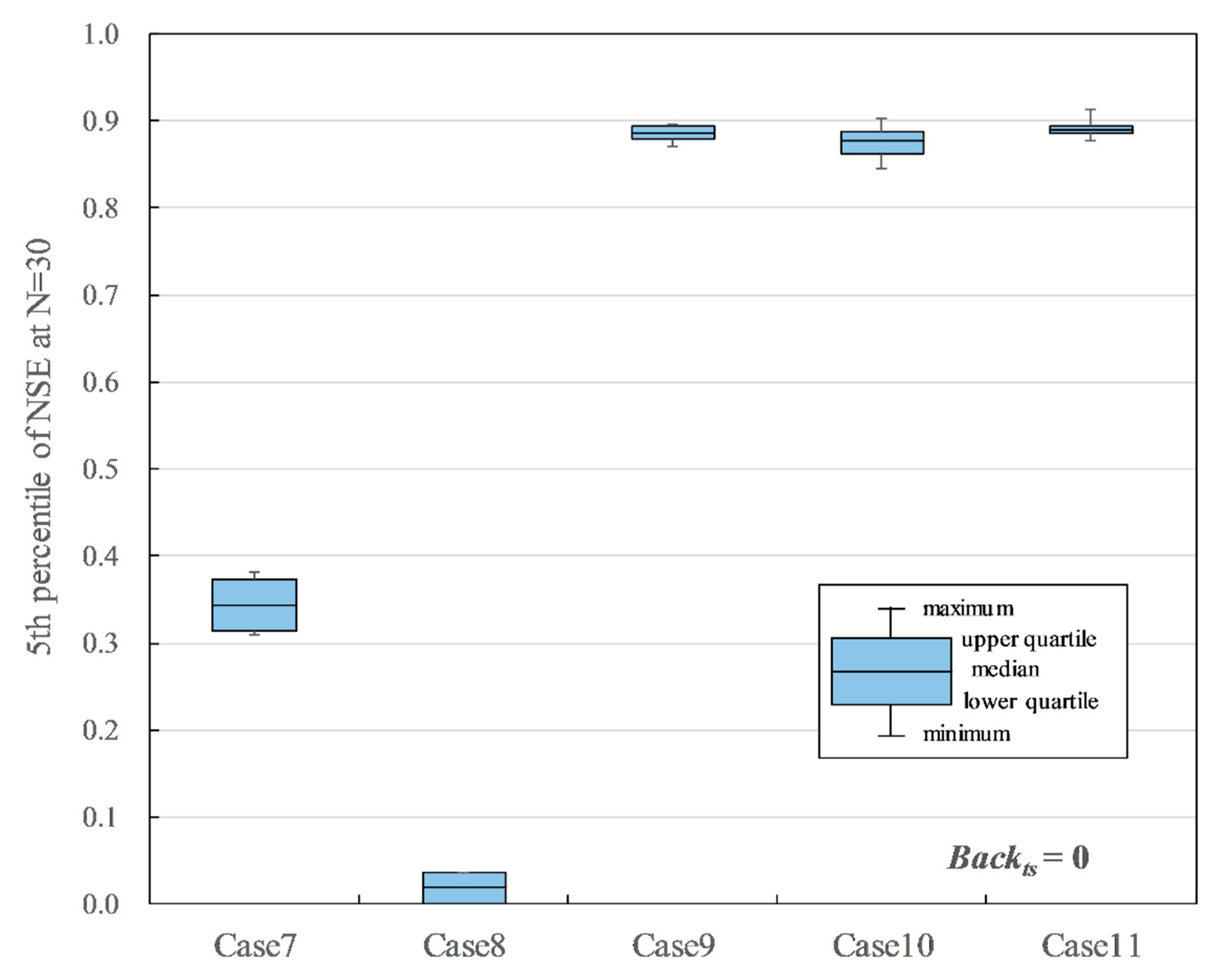
The results of the cases without the discharge data of Shioyabashi as Backts = 0 are shown in Figure 11. Case 9, Case 10, and Case 11, which used discharge data of Sanpukuji as the input data, indicated relatively good accuracies. However, they were 0.877–0.891 in the median of P5 of NSE, which was slightly less than the reference accuracy. In Case 7, where only precipitation was used as the input data, the median of the P5 of NSE is 0.344. In Case 8, where only air temperature was used as the input data, the median of the P5 of NSE is 0.013, indicating that it is difficult to estimate the missing data. These results suggest the understanding for the input data combination is: (i) both the Sanpukuji data and the Shioyabashi data are necessary; (ii) air temperature is not required; and (iii) precipitation may contribute to the improvement of accuracy, but it should be noted that it may cause poor accuracy depending on the parameter settings.
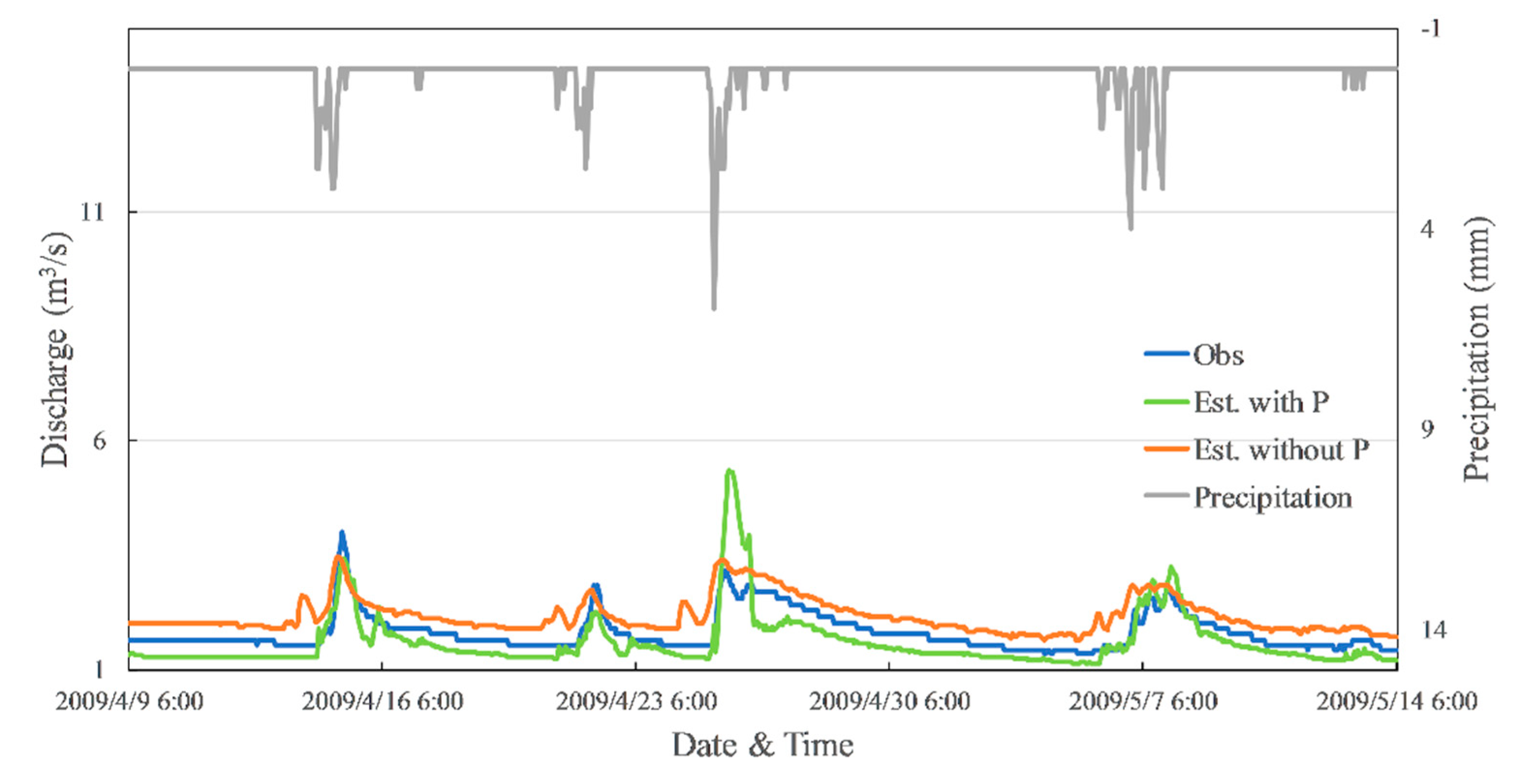
Two trainings of Case 1 (Backts = 24, Hid = 20, Drp = 0, Drpr = 0) and Case 8 (Backts = 24, Hid = 20, Drp = 0, Drpr = 0) were chosen to investigate the impact of precipitation to the estimation results. The hydrograph of observed discharge, precipitation, and both estimation results are shown in Figure 12. The blue line is observed data, and the grey line is precipitation. The green and orange lines represent discharge estimated from data with precipitation and without precipitation, respectively. The hydrograph indicates that both estimation results are responsive to precipitation events. When precipitation data was used for training, there is a trend of an occurrence of trough in the estimated discharge after a peak caused by precipitation. Additionally, the model could not estimate the discharge well when a relatively heavy precipitation event occurs. These are considered as part of the reasons that precipitation may cause lower accuracy.
3.4. Dropout and Recurrent Dropout
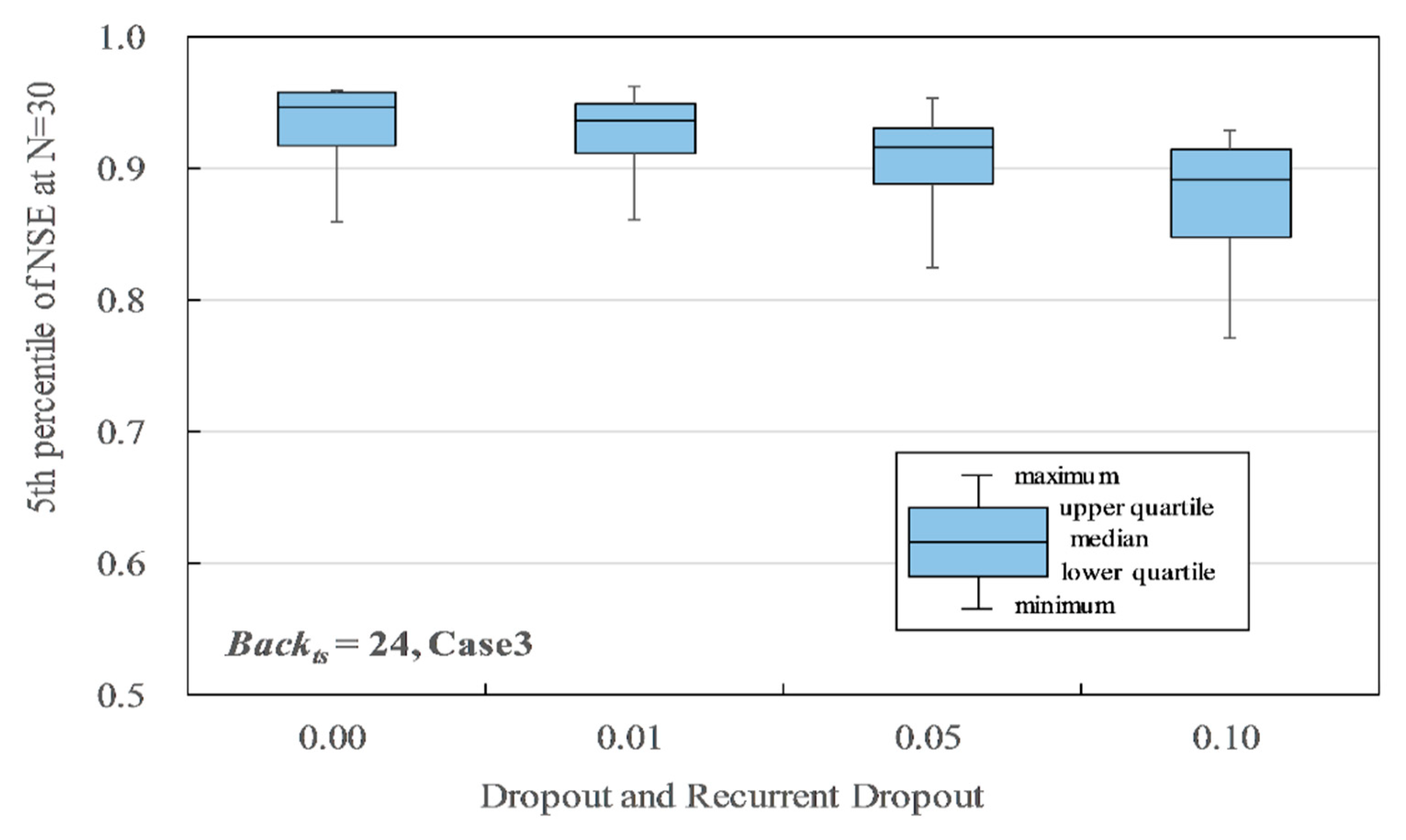
Figure 13 shows the influence of dropout and recurrent dropout (Drp&Drpr), when Hid = 20 to 200 and Backts = 24 for Case 3. The accuracy improved as Drp&Drpr became smaller, and Drp&Drpr = 0.00 had the best accuracy of 0.917 in the lower quartile P5 of the NSE. The maximum P5 of the NSE was 0.961 when Drp&Drpr = 0.01 and Hid = 200. When Hid = 20, the minimums were indicated as 0.860, 0.860, 0.825, and 0.771 for Drp&Drpr = 0.00, 0.01, 0.05, and 0.10, respectively. When Drp&Drpr = 0.00 or 0.01, in the case of Hid > 50, the accuracies were indicated to be more than 0.920, which is over the reference accuracy. In brief, Drp&Drpr = 0.00 shows the best results. The reason may be that higher Drp and Drpr values drop more units for the linear transformation of the input and recurrent state. Fewer units caused a shortage of information necessary for the training, since the LSTM model of this study has only a few units in the input and hidden layers. In the case of some other studies, a large number of units in the input and hidden layers caused drops in the units by dropout and recurrent dropout, which improved the training results [32,33]. Thus, if Hid is less than 200, Drp&Drpr = 0.00 is appropriate, and if Hid is more than 200, Drp&Drpr = 0.01 is appropriate.
3.5. Number of Hidden Layers
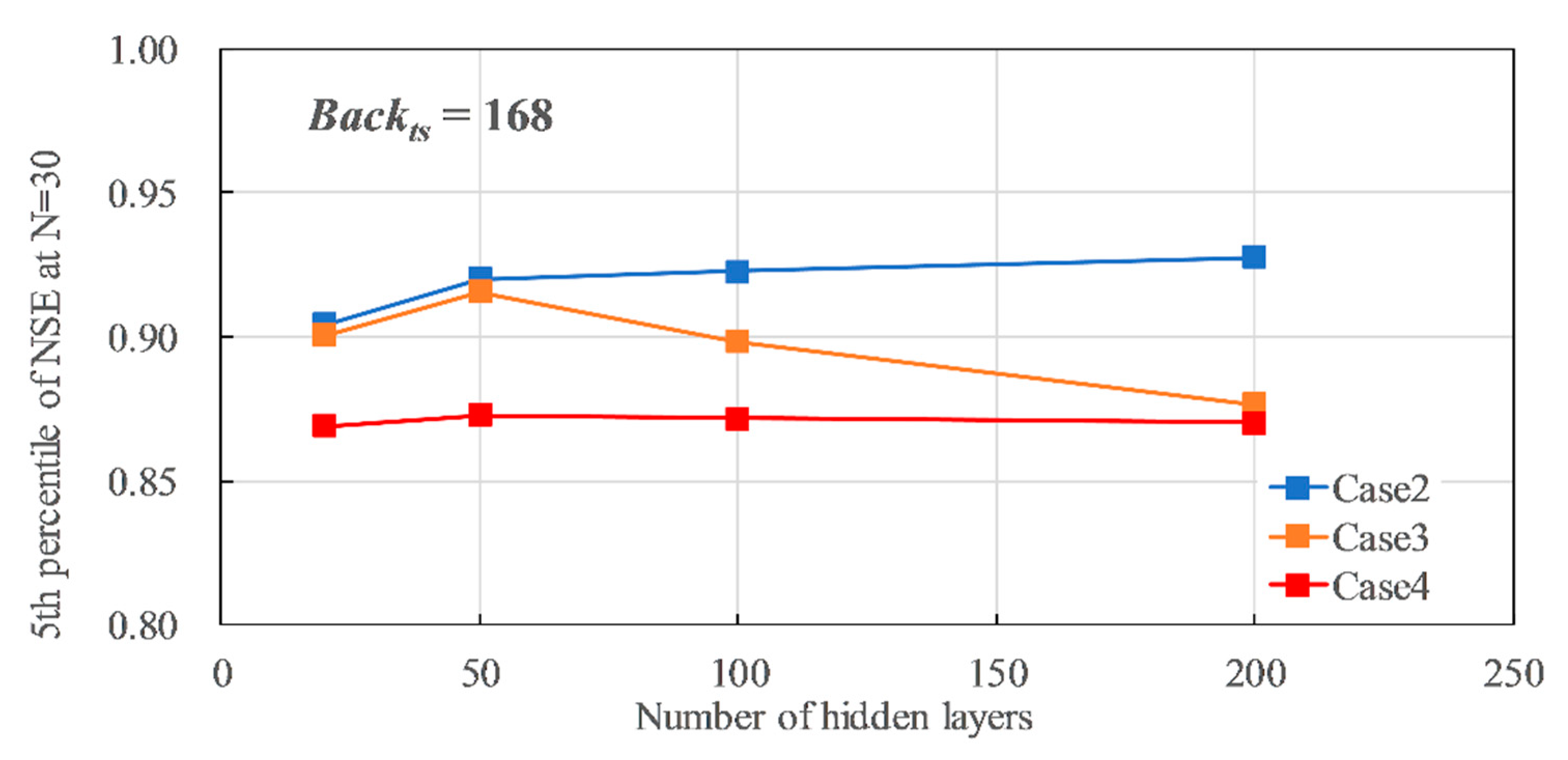
Figure 14 shows the relationship between the number of hidden layers (Hid = 20 to 200) and the P5 of NSE, when Backts = 24 and Drp&Drpr = 0.00. In Cases 2, 3, and 4, the accuracy improved as Hid increased. Case 2 and 3 indicated better accuracy than the reference accuracy 0.903 when Hid > 50. However, when Hid > 100, the accuracies were almost the same, i.e., 0.947–0.947 for Case 2, 0.957–0.959 for Case 3. Additionally, Figure 15 shows the relationship between the number of hidden layers (Hid = 20 to 200) and the P5 of the NSE when Backts = 168 and Drp&Drpr = 0.00. In Case 2, the accuracy slightly improved from 0.904 to 0.928 as Hid increased. In Case 4, the accuracy had almost no change as Hid increased. On the other hand, in Case 3, Hid = 50 indicated the best accuracy of 0.915. However, the accuracy decreased as Hid increased when Hid > 50. In Case 3, with precipitation as the input, the estimated hydrograph might be jagged due to the influence of precipitation, showing pulsed time-series data. This is the reason why Case 3 does not always show the best accuracy. As a result, for Backts = 24, Hid = 100 is appropriate for both Cases 2 and 3 because the accuracies for Hid = 100 and 200 were almost same. Setting a higher Hid value will just lead to a longer training time consumption. Moreover, for Backts = 168, Hid = 100 is also appropriate for Case 2, and Hid = 50 is appropriate for Case 3. However, in Case 3, where precipitation is used as the input data, care should be taken because the accuracy may decrease depending on the settings.
4. Conclusions
In this study, LSTM was applied for the imputation of missing discharge data of the Daihachiga River. The performance of an LSTM model was evaluated, and the hyperparameters of the model were tuned to satisfy the reference accuracy of 0.903 in NSE. Different hyperparameters affect the model performance to different extents. In the case of the Daihachiga River, the discharge data of both observation points should be included in input variables for training (Case 2). It is thought that the discharge data of Shioyabashi dating back 1 day or 7 days is effective in correcting the absolute value of the estimated discharge, because the estimated hydrograph with Case 9 had a slight error in base flow volume. The influence of precipitation varies. Since precipitation is strongly related to discharge, it may be useful to complete missing data. However, there is a possibility of making the estimated hydrograph jagged due to the influence of precipitation, showing pulsed time-series data. Although it is possible that filtering the precipitation data before inputting it into the LSTM will improve the accuracy, it is safer to exclude precipitation data in order to obtain consistently good results. Moreover, air temperature data could not improve the performance. Due to the small number of units for transformation in the model of this study, setting the dropout value to 0 was suitable. A higher Hid value might be more suitable for the model. However, an excessive Hid value would just lead to a longer training time.
Consequently, this study can propose the hyperparameter settings as In = Case 2, Hid = 100, Drp&Drpr = 0, a setting with which it is possible to estimate with greater accuracy than the reference. The necessity of hyperparameter tuning was proved, and the hyperparameter settings could be a reference for further research in relevant areas. Of course, this combination can be appropriately adjusted under specific experimental conditions. In future experiments, the amount of analysis data can be increased, such as the discharge data of more than two observation points, and the influence of precipitation and air temperature on the model performance can be further analyzed to improve the accuracy of the results.
Supplementary Materials
The following are available online at https://www.mdpi.com/article/10.3390/w14020213/s1, Table S1: 90 kinds of hyperparameter combination.
Author Contributions
W.: Conceptualization, methodology, software, validation, formal analysis, investigation, resources, data curation, writing—original draft preparation, writing—review and editing; T.K.: conceptualization, methodology, software, investigation, resources, writing—review and editing, project administration, funding acquisition. All authors have read and agreed to the published version of the manuscript.
Funding
This work was supported by JSPS KAKENHI (Grant Numbers JP20K04747, JP20K12284).
Institutional Review Board Statement
Not applicable.
Informed Consent Statement
Not applicable.
Data Availability Statement
Data are contained within the article and supplementary material. Raw data are available on request from the corresponding author.
Acknowledgments
The authors thank the Miya River Upper Reaches Development and Construction Work Office, Gifu Prefecture, for providing the discharge data of the Daihachiga River in this study.
Conflicts of Interest
The authors declare no conflict of interest.
References
- Gao, Y.; Merz, C.; Lischeid, G.; Schneider, M. A Review on Missing Hydrological Data Processing. Environ. Earth Sci. 2018, 77, 47. [Google Scholar] [CrossRef]
- Kojiri, T.; Panu, U.S.; Tomosugi, K. Complement Method of Observation Lack of Discharge with Pattern Classification and Fuzzy Inference. J. Jpn. Soc. Hydrol. Water Resour. 1994, 7, 536–543. [Google Scholar] [CrossRef]
- Tezuka, M.; Ohgushi, K. A Practical Method To Estimate Missing. In Proceedings of the 18th IAHR APD Congress, Jeju, Korean, 22–23 August 2012; pp. 547–548. [Google Scholar]
- Ding, Y.; Zhu, Y.; Feng, J.; Zhang, P.; Cheng, Z. Interpretable Spatio-Temporal Attention LSTM Model for Flood Forecasting. Neurocomputing 2020, 403, 348–359. [Google Scholar] [CrossRef]
- Li, W.; Kiaghadi, A.; Dawson, C. Exploring the Best Sequence LSTM Modeling Architecture for Flood Prediction. Neural Comput. Appl. 2020, 33, 5571–5580. [Google Scholar] [CrossRef]
- Le, X.H.; Ho, H.V.; Lee, G.; Jung, S. Application of Long Short-Term Memory (LSTM) Neural Network for Flood Forecasting. Water 2019, 11, 1387. [Google Scholar] [CrossRef] [Green Version]
- Taniguchi, J.; Kojima, T.; Sota, Y.; Hukumoto, S.; Satou, H.; Machida, Y.; Mikami, T.; Nagayama, M.; Nishikohri, T.; Watanabe, A. Application of Recurrent Neural Network for Dam Inflow Prediction. Adv. River Eng. 2019, 25, 321–326. [Google Scholar]
- Hu, C.; Wu, Q.; Li, H.; Jian, S.; Li, N.; Lou, Z. Deep Learning with a Long Short-Term Memory Networks Approach for Rainfall-Runoff Simulation. Water 2018, 10, 1543. [Google Scholar] [CrossRef] [Green Version]
- Xiang, Z.; Yan, J.; Demir, I. A Rainfall-Runoff Model With LSTM-Based Sequence-to-Sequence Learning. Water Resour. Res. 2020, 56, e2019WR025326. [Google Scholar] [CrossRef]
- Sahoo, B.B.; Jha, R.; Singh, A.; Kumar, D. Long Short-Term Memory (LSTM) Recurrent Neural Network for Low-Flow Hydrological Time Series Forecasting. Acta Geophys. 2019, 67, 1471–1481. [Google Scholar] [CrossRef]
- Sudriani, Y.; Ridwansyah, I.; Rustini, H.A. Long Short Term Memory (LSTM) Recurrent Neural Network (RNN) for Discharge Level Prediction and Forecast in Cimandiri River, Indonesia. In Proceedings of the IOP Conference Series: Earth and Environmental Science; Institute of Physics Publishing: Bristol, UK, 2019; Volume 299. [Google Scholar]
- Lee, G.; Lee, D.; Jung, Y.; Kim, T.-W. Comparison of Physics-Based and Data-Driven Models for Streamflow Simulation of the Mekong River. J. Korea Water Resour. Assoc. 2018, 51, 503–514. [Google Scholar] [CrossRef]
- Bai, P.; Liu, X.; Xie, J. Simulating Runoff under Changing Climatic Conditions: A Comparison of the Long Short-Term Memory Network with Two Conceptual Hydrologic Models. J. Hydrol. 2021, 592, 125779. [Google Scholar] [CrossRef]
- Fan, H.; Jiang, M.; Xu, L.; Zhu, H.; Cheng, J.; Jiang, J. Comparison of Long Short Term Memory Networks and the Hydrological Model in Runoff Simulation. Water 2020, 12, 175. [Google Scholar] [CrossRef] [Green Version]
- Granata, F.; di Nunno, F. Forecasting Evapotranspiration in Different Climates Using Ensembles of Recurrent Neural Networks. Agric. Water Manag. 2021, 255, 107040. [Google Scholar] [CrossRef]
- Chen, Z.; Zhu, Z.; Jiang, H.; Sun, S. Estimating Daily Reference Evapotranspiration Based on Limited Meteorological Data Using Deep Learning and Classical Machine Learning Methods. J. Hydrol. 2020, 591, 125286. [Google Scholar] [CrossRef]
- Ferreira, L.B.; da Cunha, F.F. Multi-Step Ahead Forecasting of Daily Reference Evapotranspiration Using Deep Learning. Comput. Electron. Agric. 2020, 178, 105728. [Google Scholar] [CrossRef]
- Reimers, N.; Gurevych, I. Optimal Hyperparameters for Deep LSTM-Networks for Sequence Labeling Tasks. arXiv 2017, arXiv:1707.06799. [Google Scholar]
- Hossain, M.D.; Ochiai, H.; Fall, D.; Kadobayashi, Y. LSTM-Based Network Attack Detection: Performance Comparison by Hyper-Parameter Values Tuning. In Proceedings of the 2020 7th IEEE International Conference on Cyber Security and Cloud Computing (CSCloud)/2020 6th IEEE International Conference on Edge Computing and Scalable Cloud (EdgeCom), New York, NY, USA, 1–3 August 2020; pp. 62–69. [Google Scholar]
- Yadav, A.; Jha, C.K.; Sharan, A. Optimizing LSTM for Time Series Prediction in Indian Stock Market. Procedia Comput. Sci. 2020, 167, 2091–2100. [Google Scholar] [CrossRef]
- Yi, H.; Bui, K.N. An Automated Hyperparameter Search-Based Deep Learning Model for Highway Traffic Prediction. IEEE Trans. Intell. Transp. Syst. 2020, 22, 5486–5495. [Google Scholar] [CrossRef]
- Kratzert, F.; Klotz, D.; Shalev, G.; Klambauer, G.; Hochreiter, S.; Nearing, G. Benchmarking a Catchment-Aware Long Short-Term Memory Network (LSTM) for Large-Scale Hydrological Modeling. Hydrol. Earth Syst. Sci. Discuss. 2019, 2019, 1–32. [Google Scholar] [CrossRef]
- Afzaal, H.; Farooque, A.A.; Abbas, F.; Acharya, B.; Esau, T. Groundwater Estimation from Major Physical Hydrology Components Using Artificial Neural Networks and Deep Learning. Water 2020, 12, 5. [Google Scholar] [CrossRef] [Green Version]
- Ayzel, G.; Heistermann, M. The Effect of Calibration Data Length on the Performance of a Conceptual Hydrological Model versus LSTM and GRU: A Case Study for Six Basins from the CAMELS Dataset. Comput. Geosci. 2021, 149, 104708. [Google Scholar] [CrossRef]
- Alizadeh, B.; Ghaderi Bafti, A.; Kamangir, H.; Zhang, Y.; Wright, D.B.; Franz, K.J. A Novel Attention-Based LSTM Cell Post-Processor Coupled with Bayesian Optimization for Streamflow Prediction. J. Hydrol. 2021, 601, 126526. [Google Scholar] [CrossRef]
- Kojima, T.; Weilisi; Ohashi, K. Investigation of Missing River Discharge Data Imputation Method Using Deep Learning. Adv. River Eng. 2020, 26, 137–142. [Google Scholar]
- River Division of Gifu Prefectural Office. Ojima Dam. Available online: https://www.pref.gifu.lg.jp/page/67841.html (accessed on 7 January 2022).
- Kojima, T.; Shinoda, S.; Mahboob, M.G.; Ohashi, K. Study on Improvement of Real-Time Flood Forecasting with Rainfall Interception Model. Adv. River Eng. 2012, 18, 435–440. [Google Scholar]
- Gers, F.A.; Schmidhuber, J.A.; Cummins, F.A. Learning to Forget: Continual Prediction with LSTM. Neural Comput. 2000, 12, 2451–2471. [Google Scholar] [CrossRef]
- Hochreiter, S.; Schmidhuber, J. Long Short-Term Memory. Neural Comput. 1997, 9, 1735–1780. [Google Scholar] [CrossRef] [PubMed]
- Nash, J.E.; Sutcliffe, J.V. River Flow Forecasting through Conceptual Models Part I—A Discussion of Principles. J. Hydrol. 1970, 10, 282–290. [Google Scholar] [CrossRef]
- Semeniuta, S.; Severyn, A.; Barth, E. Recurrent Dropout without Memory Loss. In Proceedings of the COLING 2016, the 26th International Conference on Computational Linguistics: Technical Papers, Osaka, Japan, 11–16 December 2016; Matsumoto, Y., Prasad, R., Eds.; The COLING 2016 Organizing Committee: Osaka, Japan, 2016; pp. 1757–1766. [Google Scholar]
- Gal, Y.; Ghahramani, Z. A Theoretically Grounded Application of Dropout in Recurrent Neural Networks. In Proceedings of the 30th International Conference on Neural Information Processing Systems (NIPS’16), Barcelona, Spain, 5–10 December 2016; Curran Associates Inc.: Barcelona, Spain, 2016; pp. 1027–1035. [Google Scholar]
Figure 1.
The Daihachiga River Basin and observation points. (a) Location of Gifu Prefecture; (b) location of the Daihachiga River Basin; (c) observation points of the Daihachiga River.
Figure 1.
The Daihachiga River Basin and observation points. (a) Location of Gifu Prefecture; (b) location of the Daihachiga River Basin; (c) observation points of the Daihachiga River.

Figure 2.
Structure of LSTM model.

Figure 3.
Linear regression model estimated with 2008 data.

Figure 4.
Tank model estimated with 2009 precipitation data.

Figure 5.
Relationship between RMSE, MAE, and NSE.

Figure 6.
Hydrograph of Training No. 2.

Figure 7.
Hydrograph of Training No. 3.

Figure 8.
Examples of relationship between number of ensemble members (N) and 5th percentile of NSE for Case 2. Blue line: Backts = 24, Hid = 20, Drp = 0, Drpr = 0; orange line: Backts = 24, Hid = 200, Drp = 0, Drpr = 0; red line: Backts = 168, Hid = 100, Drp = 0, Drpr = 0.
Figure 8.
Examples of relationship between number of ensemble members (N) and 5th percentile of NSE for Case 2. Blue line: Backts = 24, Hid = 20, Drp = 0, Drpr = 0; orange line: Backts = 24, Hid = 200, Drp = 0, Drpr = 0; red line: Backts = 168, Hid = 100, Drp = 0, Drpr = 0.

Figure 9.
Summarized training results for Case 1 to Case 6 when Backts = 24, Drp = 0, Drpr = 0.

Figure 10.
Summarized training results for Case 1 to Case 6 when Backts = 168, Drp = 0, Drpr = 0.

Figure 11.
Summarized training results for Case 7 to Case 11 when Backts = 0, Drp = 0, Drpr = 0.

Figure 12.
Influence of precipitation on the estimation results.

Figure 13.
Influence of dropout and recurrent dropout on the 5th percentile of NSE.

Figure 14.
Influence of number of hidden layers on the 5th percentile of NSE, when Backts = 24.

Figure 15.
Influence of number of hidden layers on the 5th percentile of NSE, when Backts = 168.


Table 1.
Assigned values of hyperparameters.
| Hyperparameter | Value1 | Value2 | Value3 | Value4 |
|---|---|---|---|---|
| Backts | 24 | 168 | 0 | |
| Hid | 20 | 50 | 100 | 200 |
| Drp | 0 | 0.01 | 0.05 | 0.1 |
| Drpr | 0 | 0.01 | 0.05 | 0.1 |
Table 2.
Cases of input variables.
| Type of Input Variables | Number of Input Variables | |
|---|---|---|
| Case1 | Qshio + P | 2 |
| Case2 | Qshio + Qsan | 2 |
| Case3 | Qshio + Qsan + P | 3 |
| Case4 | Qshio + Qsan + P + T | 4 |
| Case5 | Qshio | 1 |
| Case6 | Qshio + T | 2 |
| Case7 | P | 1 |
| Case8 | T | 1 |
| Case9 | Qsan | 1 |
| Case10 | Qsan + P | 2 |
| Case11 | Qsan + T | 2 |
P: precipitation. Qsan: discharge volume of Sanpukuji. Qshio: discharge volume of Shioyabashi. T: air temperature.
Publisher’s Note: MDPI stays neutral with regard to jurisdictional claims in published maps and institutional affiliations. |
© 2022 by the authors. Licensee MDPI, Basel, Switzerland. This article is an open access article distributed under the terms and conditions of the Creative Commons Attribution (CC BY) license (https://creativecommons.org/licenses/by/4.0/).
Share and Cite
MDPI and ACS Style
Weilisi; Kojima, T. Investigation of Hyperparameter Setting of a Long Short-Term Memory Model Applied for Imputation of Missing Discharge Data of the Daihachiga River. Water 2022, 14, 213. https://doi.org/10.3390/w14020213
AMA Style
Weilisi, Kojima T. Investigation of Hyperparameter Setting of a Long Short-Term Memory Model Applied for Imputation of Missing Discharge Data of the Daihachiga River. Water. 2022; 14(2):213. https://doi.org/10.3390/w14020213
Chicago/Turabian StyleWeilisi, and Toshiharu Kojima. 2022. "Investigation of Hyperparameter Setting of a Long Short-Term Memory Model Applied for Imputation of Missing Discharge Data of the Daihachiga River" Water 14, no. 2: 213. https://doi.org/10.3390/w14020213
Note that from the first issue of 2016, this journal uses article numbers instead of page numbers. See further details here.