
Study on the Optimal Operation of a Hydropower Plant Group Based on the Stochastic Dynamic Programming with Consideration for Runoff Uncertainty

 ,
,
Abstract
:1. Introduction
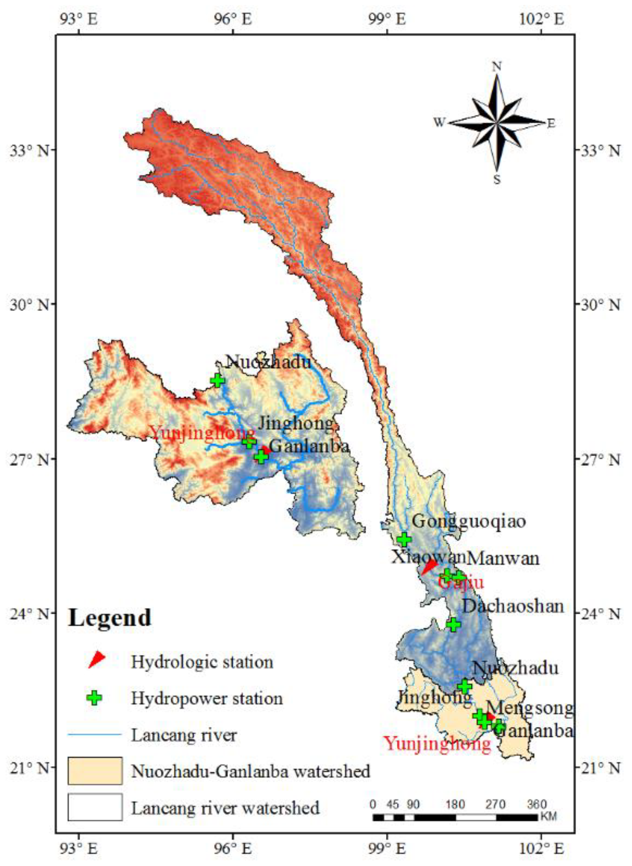
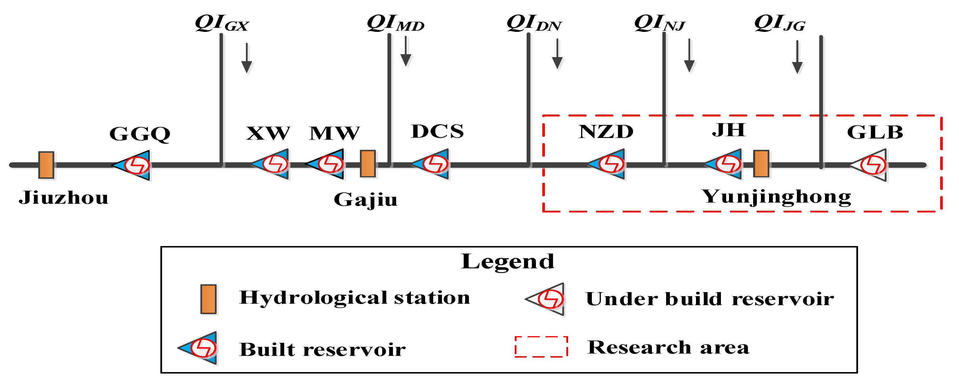
2. Study Area and Data
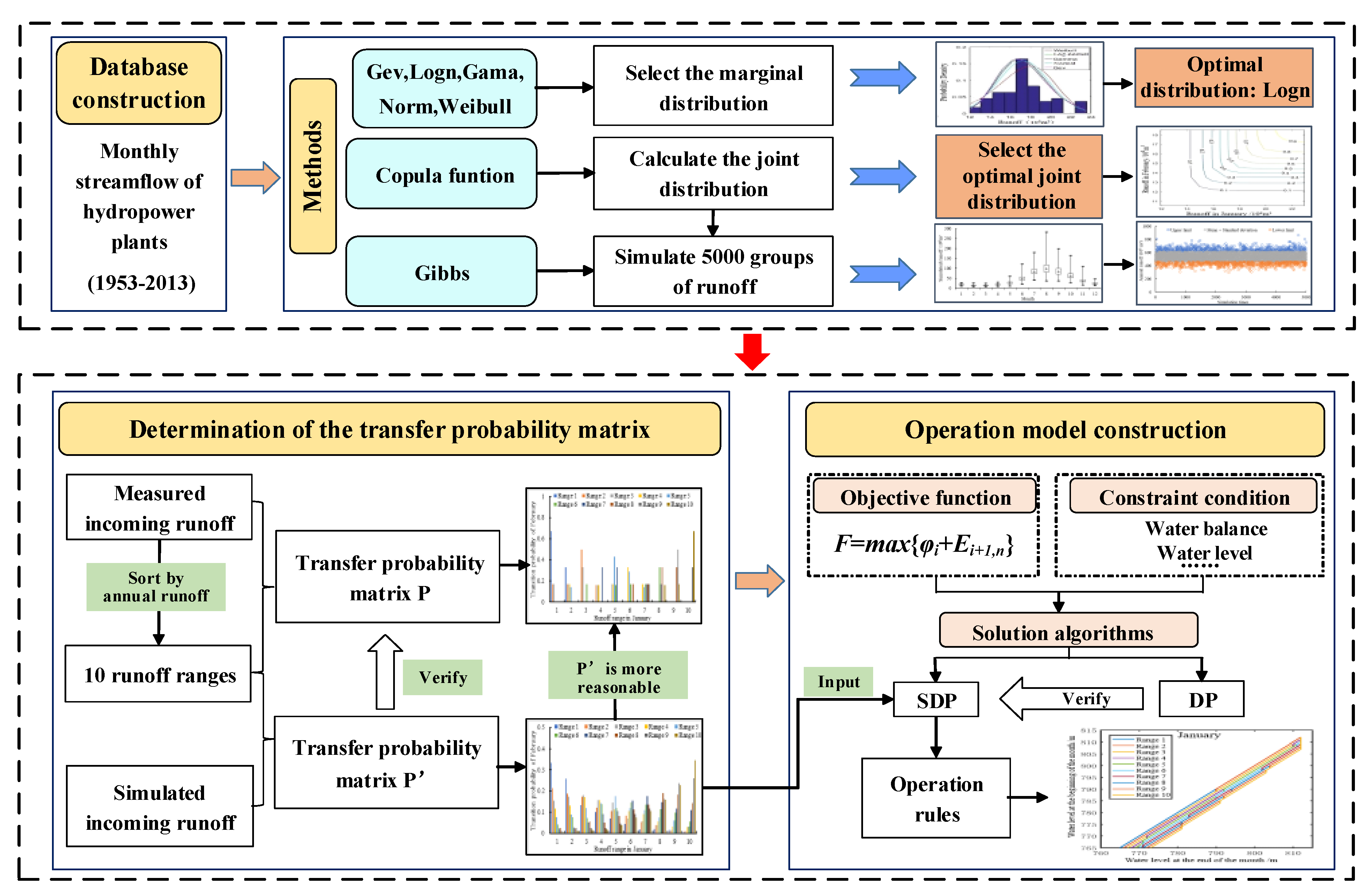
3. Methods
3.1. Construction of Joint Distribution Model for Monthly Runoff
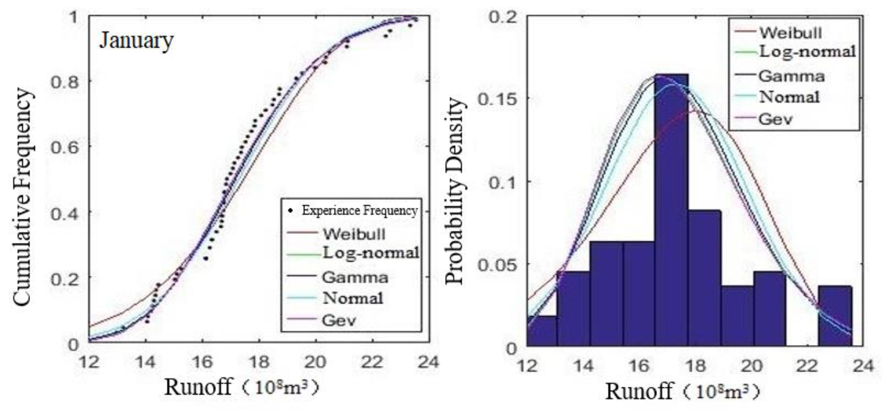
3.1.1. Marginal Distribution Model of Incoming Runoff
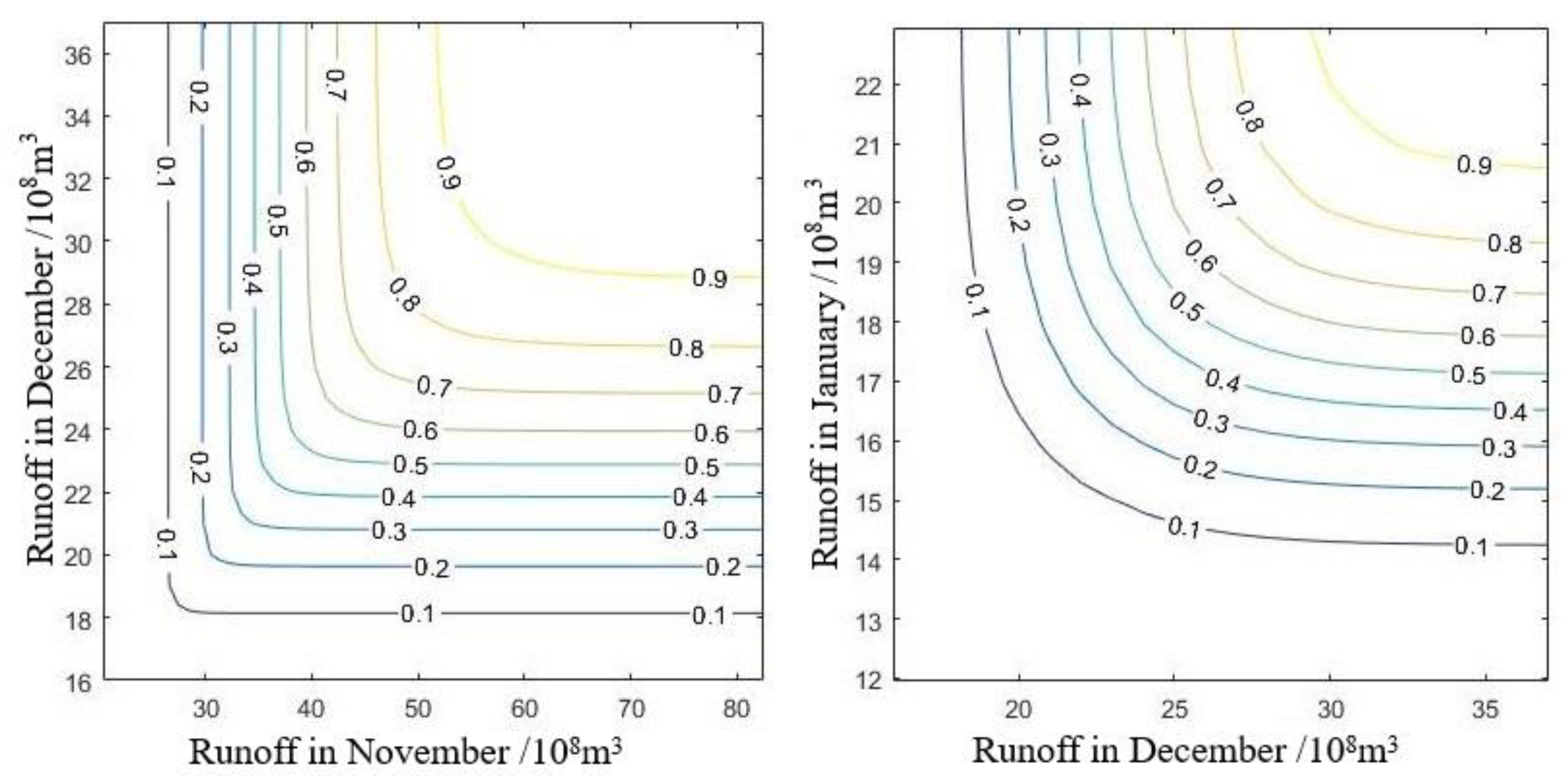
3.1.2. Joint Distribution Model of Adjacent Monthly Incoming Runoff
3.2. Stochastic Simulation Model of Runoff
3.3. Construction of Stochastic Operation Model and Solution
3.3.1. Objective Function
3.3.2. Constraint Condition
- Water balance constraint:
- Discharge constraint:
- Water level constraint:
- Output constraint:
- The minimum ecological flow constraints:
- The minimum shipping flow constraints:
3.3.3. Solution Algorithm
4. Results and Discussion
4.1. Stochastic Simulation of Runoff
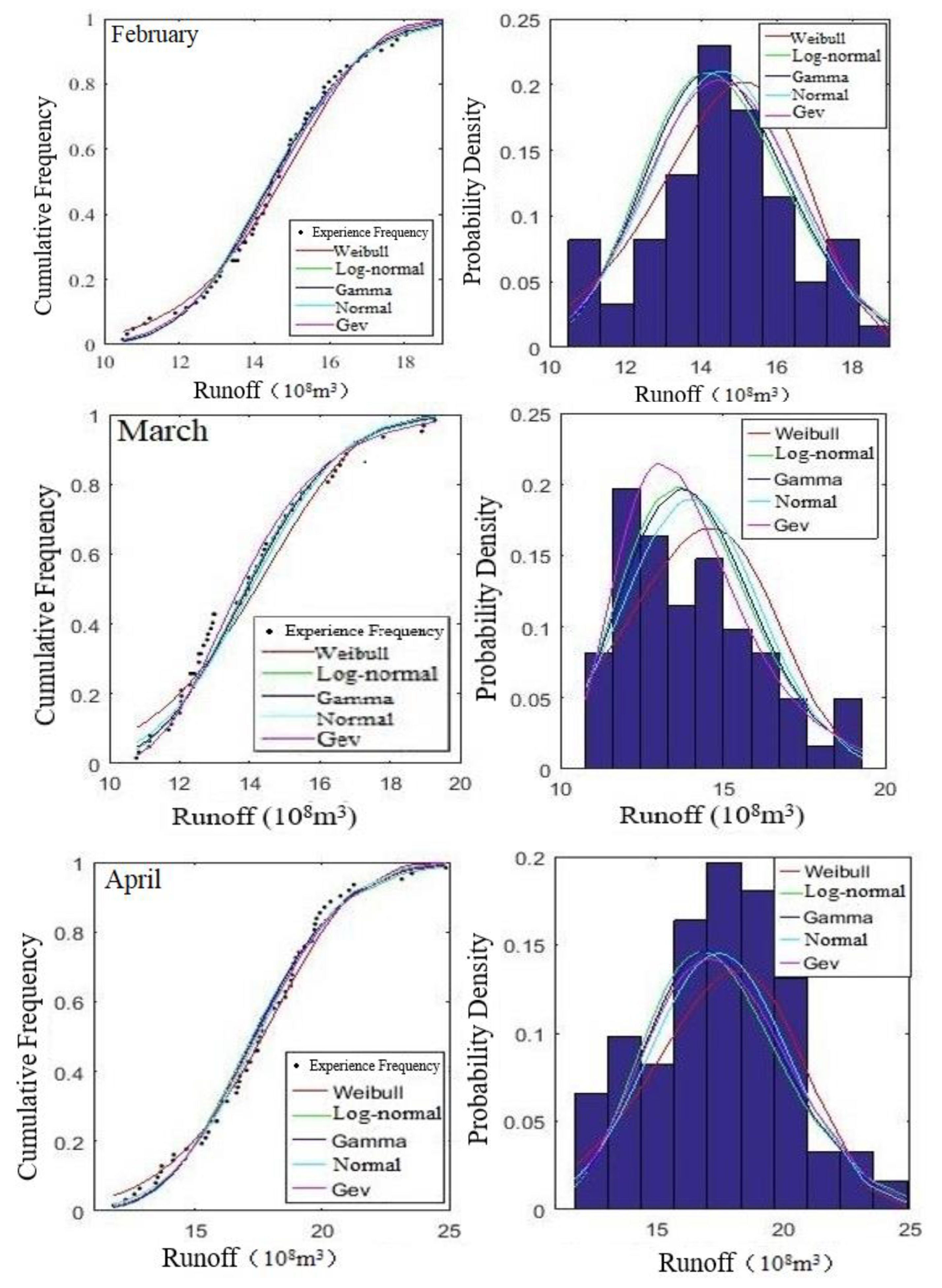
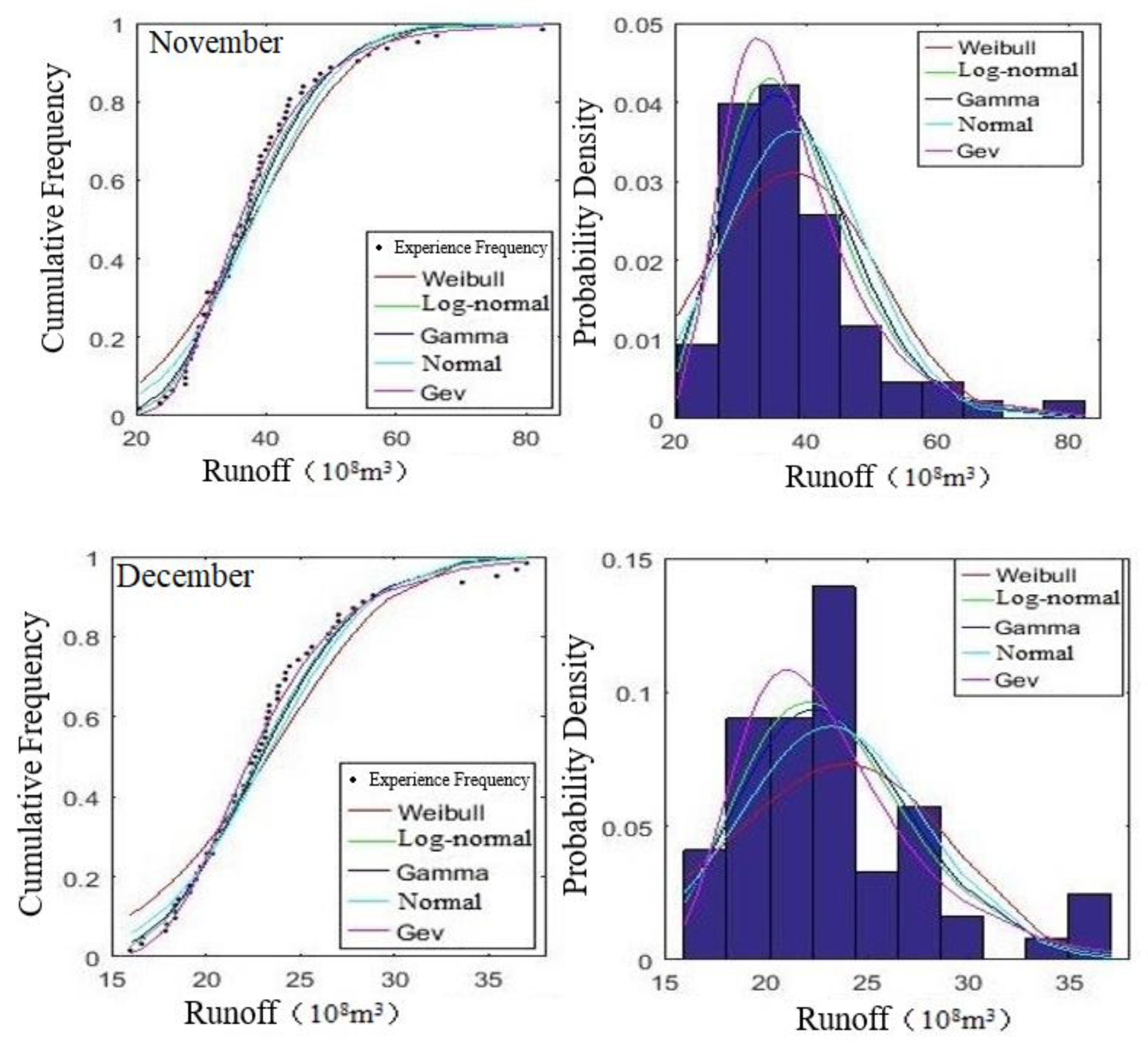
4.1.1. Marginal Distribution for Incoming Runoff
4.1.2. Copula Joint Distribution for Incoming Runoff
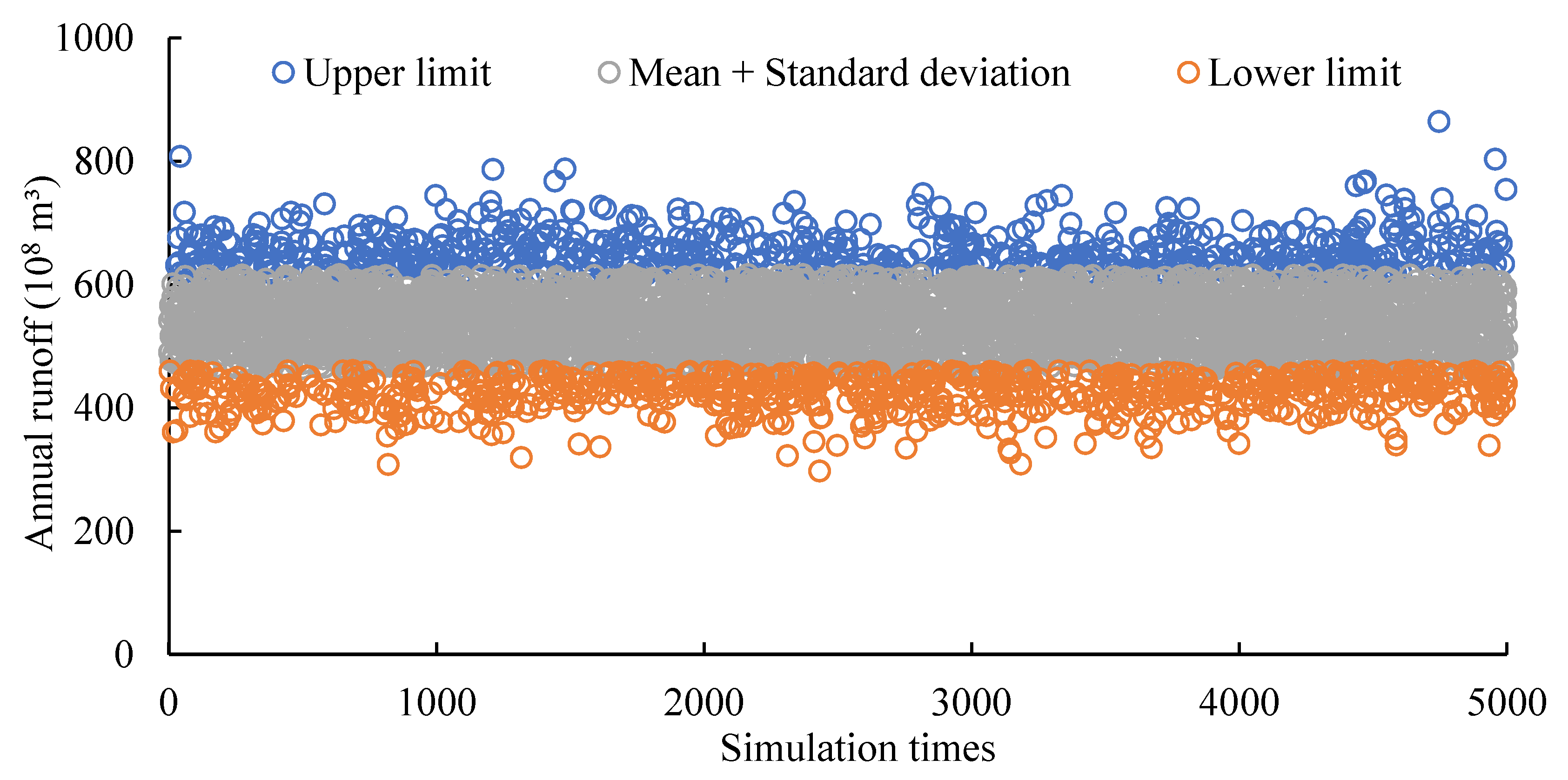
4.1.3. Stochastic Simulation of Incoming Runoff
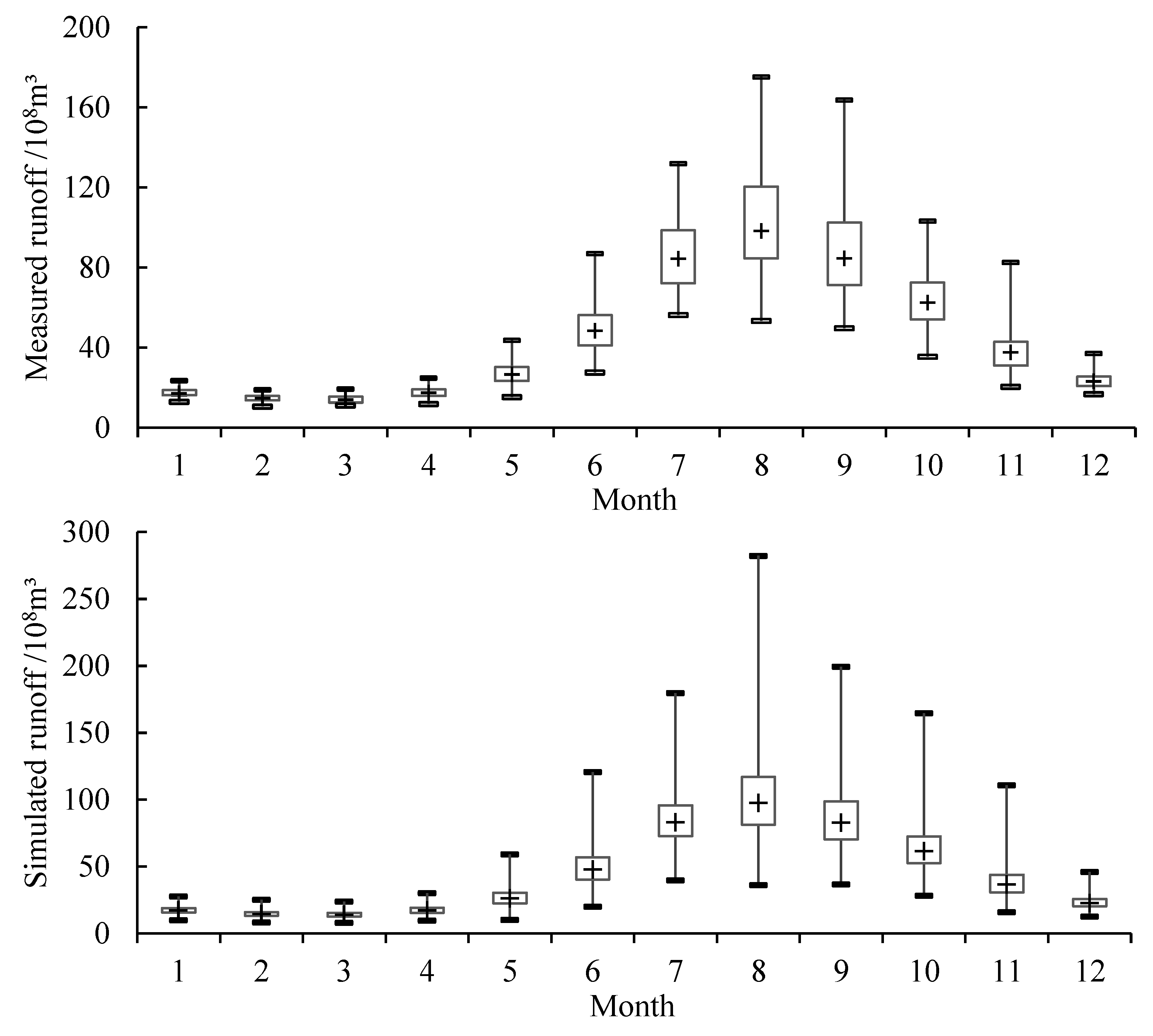
4.2. Process of Incoming Runoff
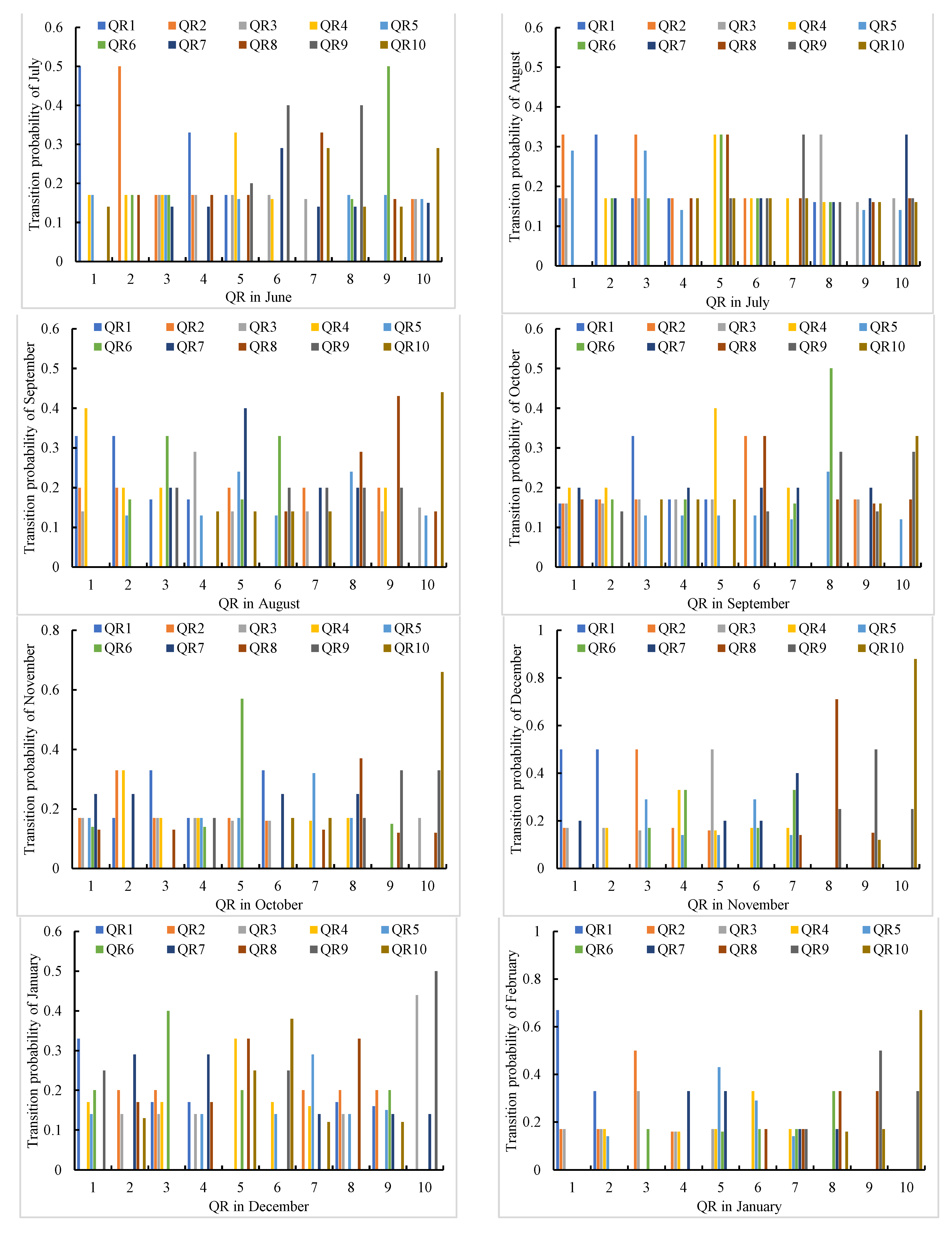
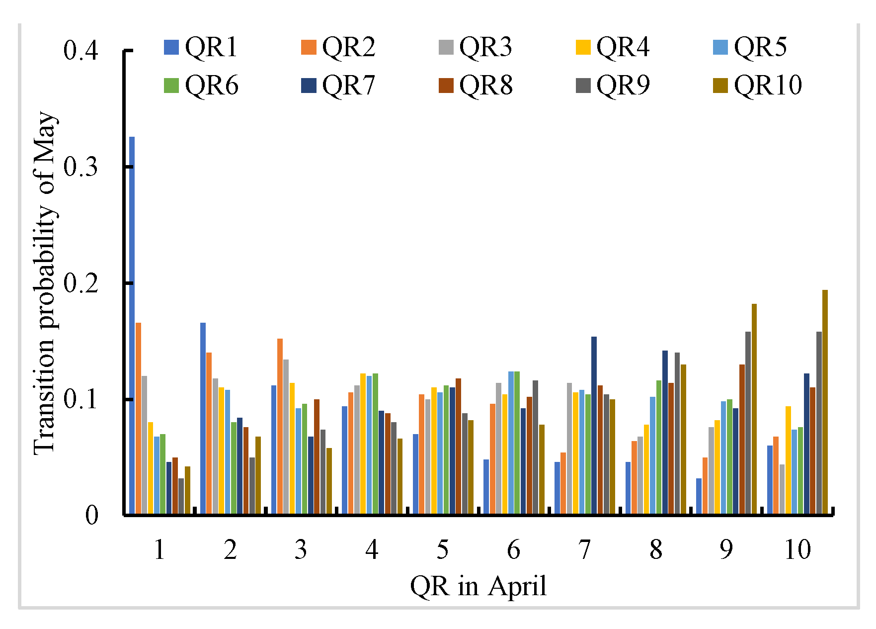
4.2.1. Transfer Probability Matrix Based on Measured Runoff
4.2.2. Transfer Probability Matrix based on Simulated Runoff
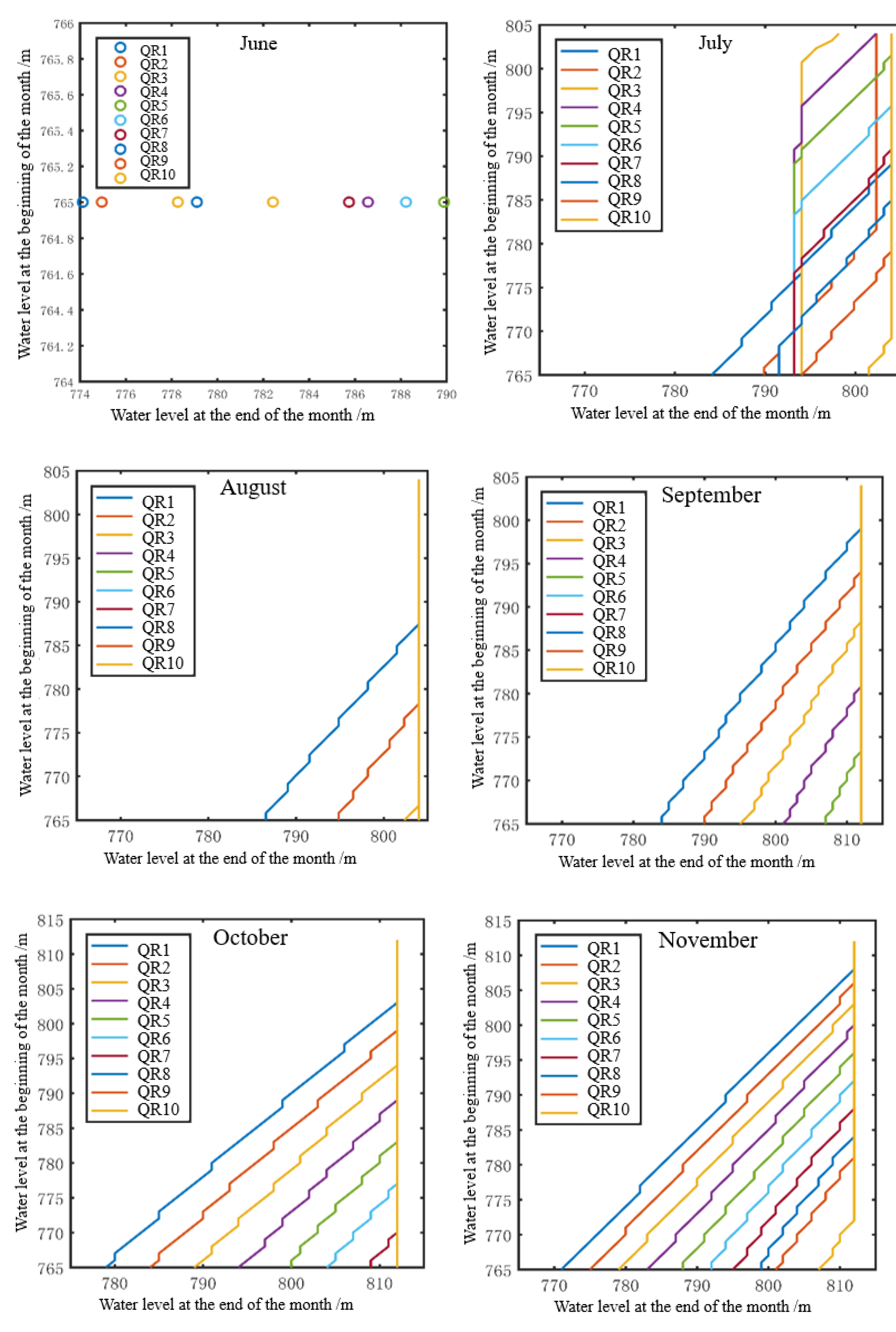
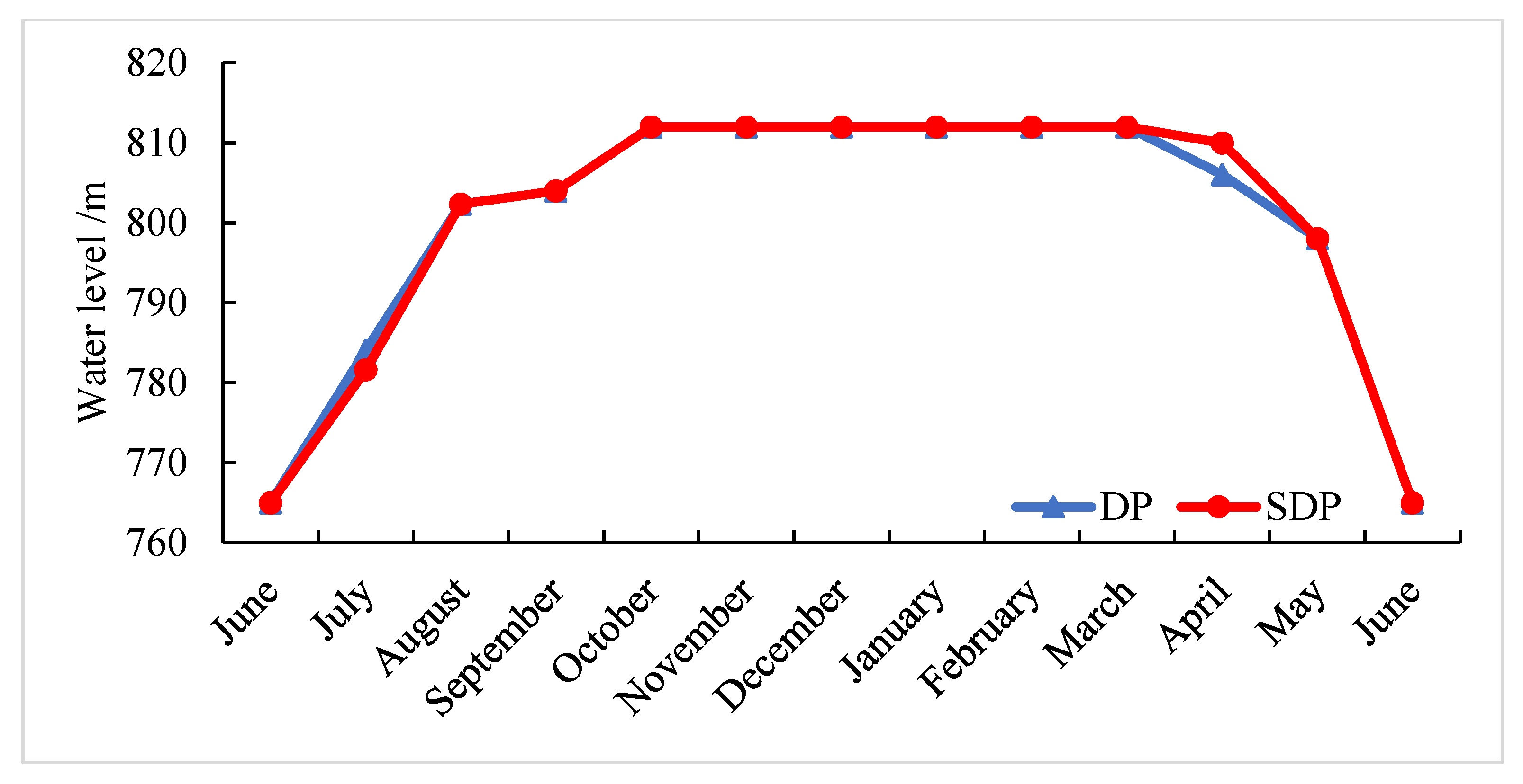
4.3. Result of Hydropower Plants Operation
5. Conclusions
Author Contributions
Funding
Institutional Review Board Statement
Informed Consent Statement
Conflicts of Interest
References
- Chang, J.; Meng, X.; Wang, Z.; Wang, X.; Huang, Q. Optimized cascade reservoir operation considering ice flood control and power generation. J. Hydrol. 2014, 519, 1042–1051. [Google Scholar] [CrossRef]
- Chang, J.; Guo, A.; Du, H.; Wang, Y. Floodwater utilization for cascade reservoirs based on dynamic control of seasonal flood control limit levels. Environ. Earth Sci. 2017, 76, 260. [Google Scholar] [CrossRef]
- Zhang, L.; Huang, Q.; Liu, D.; Deng, M.; Zhang, H.; Pan, B.; Zhang, H. Long-term and mid-term ecological operation of cascade hydropower plants considering ecological water demands in arid region. J. Clean. Prod. 2021, 279, 123599. [Google Scholar] [CrossRef]
- Wang, Y.M.; Chang, J.; Huang, Q. Simulation with RBF Neural Network Model for Reservoir Operation Rules. Water Resour. Manag. 2010, 24, 2597–2610. [Google Scholar] [CrossRef]
- Ponnambalam, K.; Vannelli, A.; Unny, T.E. An application of Karmarkar’s interior-point linear programming algorithm for multi-reservoir operations optimization. Stoch. Hydrol. Hydraul. 1989, 3, 17–29. [Google Scholar] [CrossRef]
- Oliveira, R.; Loucks, D.P. Operating rules for multi-reservoir systems. Water Resour. Res. 1997, 33, 839–852. [Google Scholar] [CrossRef]
- Chandramouli, V.; Raman, H. Multireservoir modeling with dynamic programming and neural networks. J. Water Resour. Plan. Manag. 2001, 127, 89–98. [Google Scholar]
- Arunkumar, R.; Jothiprakash, V. Chaotic evolutionary algorithms for multi-reservoir optimization. Water Resour. Manag. 2013, 27, 5207–5222. [Google Scholar] [CrossRef]
- Na, Y.; Ke, Z.; Yang, H.; Zhao, Q.; Huang, Q.; Xue, Y.; Xue, X.; Chen, S. Evaluation of the TRMM multisatellite precipitation analysis and its applicability in supporting reservoir operation and water resources management in Hanjiang basin, China. J. Hydrol. 2017, 549, 313–325. [Google Scholar]
- Li, L.; Xu, H.; Chen, X.; Simonovic, S.P. Streamflow Forecast and Reservoir Operation Performance Assessment under Climate Change. Water Resour. Manag. 2010, 24, 83–104. [Google Scholar] [CrossRef]
- Tegegne, G.; Kim, Y.O. Representing inflow uncertainty for the development of monthly reservoir operations using genetic algorithms. J. Hydrol. 2020, 586, 124876. [Google Scholar] [CrossRef]
- Xu, B.; Huang, X.; Zhong, P.; Wu, Y. Two-phase risk hedging rules for informing conservation of flood resources in reservoir operation considering inflow forecast uncertainty. Water Resour. Manag. 2020, 34, 2731–2752. [Google Scholar] [CrossRef]
- Galletti, A.; Avesani, D.; Bellin, A.; Majone, B. Detailed simulation of storage hydropower systems in large Alpine watersheds. J. Hydrol. 2021, 603 Pt D, 127125. [Google Scholar] [CrossRef]
- Brekke, L.D.; Maurer, E.P.; Anderson, J.D.; Dettinger, M.D.; Townsley, E.S.; Harrison, A.; Pruitt, T. Assessing reservoir operations risk under climate change. Water Resour. Res. 2009, 45, 546–550. [Google Scholar] [CrossRef] [Green Version]
- Celeste, A.B.; Billib, M. Evaluation of stochastic reservoir operation optimization models. Adv. Water Resour. 2009, 32, 1429–1443. [Google Scholar] [CrossRef]
- Archibald, T.W.; Buchanan, C.S.; Mckinnon, K.; Thomas, L. Nested Benders decomposition and dynamic programming for reservoir optimisation. J. Oper. Res. Soc. 1999, 50, 468–479. [Google Scholar] [CrossRef]
- Kumar, D.N.; Baliarsingh, F. Folded dynamic programming for optimal operation of multireservoir system. Water Resour. Manag. 2003, 17, 337–353. [Google Scholar] [CrossRef]
- Ganji, A.; Khalili, D.; Karamouz, M.; Ponnambalam, K.; Javan, M. A Fuzzy Stochastic Dynamic Nash Game Analysis of Policies for Managing Water Allocation in a Reservoir System. Water Resour. Manag. 2008, 22, 51–66. [Google Scholar] [CrossRef]
- Nikoo, M.R.; Kerachian, R.; Karimi, A.; Azadnia, A.A.; Jafarzadegan, K. Optimal water and waste load allocation in reservoir–river systems: A case study. Environ. Earth Sci. 2014, 71, 4127–4142. [Google Scholar] [CrossRef]
- Yang, Z.; Wang, Y.; Yang, K. The stochastic short-term hydropower generation scheduling considering uncertainty in load output forecasts. Energy 2022, 241, 122838. [Google Scholar] [CrossRef]
- Yang, Z.; Yan, K.; Wang, Y.; Su, L.; Hu, H. Multi-objective short-term hydropower generation operation for cascade reservoirs and stochastic decision making under multiple uncertainties. J. Clean. Prod. 2020, 276, 122995. [Google Scholar] [CrossRef]
- Little, J.D.C. The Use of Storage Water in a Hydroelectric System. J. Oper. Res. Soc. Am. 1955, 3, 187–197. [Google Scholar] [CrossRef] [Green Version]
- Howard, R.A. Dynamic Programming and Markov Processes. Math. Gaz. 1960, 3, 120. [Google Scholar]
- Rossman, L.A. Reliability constrained dynamic programing and randomized release rules in reservoir management. Water Resour. Res. 1977, 13, 247–255. [Google Scholar] [CrossRef]
- Bras, R.L.; Buchanan, R.; Curry, K.C. Real-time adaptive closed loop control of reservoirs with the High Aswan Dam as a case study. Water Resour. Res. 1983, 19, 33–52. [Google Scholar] [CrossRef]
- Saadat, M.; Asghari, K. Feasibility Improved Stochastic Dynamic Programming for Optimization of Reservoir Operation. Water Resour. Manag. 2019, 33, 3485–3498. [Google Scholar] [CrossRef]
- Shi, W.; Yu, X.; Liao, W.; Wang, Y. Spatial and temporal variability of daily precipitation concentration in the Lancang River basin, China. J. Hydrol. 2013, 495, 197–207. [Google Scholar] [CrossRef]
- Zhang, H.; Chang, J.; Gao, C.; Wu, H.; Wang, Y.; Lei, K.; Long, R.; Zhang, L. Cascade hydropower plants operation considering comprehensive ecological water demands. Energy Convers. Manag. 2019, 180, 119–133. [Google Scholar] [CrossRef]
- Ogarekpe, N.M.; Tenebe, I.T.; Emenike, P.C.; Udodi, O.; Antigha, R.E.-E. Assessment of regional best-fit probability density function of annual maximum rainfall using CFSR precipitation data. J. Earth Syst. Sci. 2020, 129, 176. [Google Scholar] [CrossRef]
- Hosseinifard, S.Z.; Abbasi, B.; Abdollahian, M. Performance Analysis in Non-Normal Linear Profiles Using Gamma Distribution. In Proceedings of the Eighth International Conference on Information Technology: New Generations, Las Vegas, NV, USA, 11–13 April 2011; IEEE: Piscataway, NJ, USA, 2011; pp. 603–607. [Google Scholar]
- Papalexiou, S.M.; Koutsoyiannis, D. A global survey on the seasonal variation of the marginal distribution of daily precipitation. Adv. Water Resour. 2016, 94, 131–145. [Google Scholar]
- Zhang, L.; Singh, V.P. Bivariate Rainfall and Runoff Analysis Using Entropy and Copula Theories. Entropy 2012, 14, 1784–1812. [Google Scholar] [CrossRef]
- Qian, L.; Wang, X.; Wang, Z. Modeling the dependence pattern between two precipitation variables using a coupled copula. Environ. Earth Sci. 2020, 79, 1–12. [Google Scholar] [CrossRef]
- Abdollahi, S.; Akhoond-Ali, A.M.; Mirabbasi, R.; Adamowski, J.F. Probabilistic Event Based Rainfall-Runoff Modeling Using Copula Functions. Water Resour. Manag. 2019, 33, 3799–3814. [Google Scholar] [CrossRef]
- Mirabbasi, R.; Fakheri-Fard, A.; Dinpashoh, Y. Bivariate drought frequency analysis using the copula method. Theor. Appl. Climatol. 2012, 108, 191–206. [Google Scholar] [CrossRef]
- Tao, S.; Sheng, D.; Wang, N.; Soares, C.G. Estimating storm surge intensity with Poisson bivariate maximum entropy distributions based on copulas. Nat. Hazards 2013, 68, 791–807. [Google Scholar] [CrossRef]
- Valle, L.D.; Giuli, M.D.; Tarantola, C.; Manelli, C. Default Probability Estimation via Pair Copula Constructions. Eur. J. Oper. Res. 2016, 249, 298–311. [Google Scholar] [CrossRef] [Green Version]
- Jackie, L. On the use of MCMC simulation for stochastic reserving. Aust. Actuar. J. 2008, 14, 227–271. [Google Scholar]
- Ma, H.; Zhu, G.; Zhang, Y.; Pan, H.; Guo, H.; Jia, W.; Zhou, J.; Yong, L.; Wan, Q. The effects of runoff on Hydrochemistry in the Qilian Mountains: A case study of Xiying River Basin. Environ. Earth Sci. 2019, 78, 1866–6280. [Google Scholar] [CrossRef]
- Nandalal, K.; Sakthivadivel, R. Planning and management of a complex water resource system: Case of Samanalawewa and Udawalawe reservoirs in the Walawe river, Sri Lanka. Agric. Water Manag. 2002, 57, 207–221. [Google Scholar] [CrossRef]
- Jha, D.K.; Yorino, N.; Zoka, Y.; Sasaki, Y.; Hayashi, Y.; Iwata, K.; Oe, R. Backward search approach to incorporate excess stream inflows in SDP based reservoir scheduling of hydropower plants. In Proceedings of the 2009 IEEE/PES Power Systems Conference & Exposition, Seattle, WA, USA, 15–18 March 2009; IEEE: Piscataway, NJ, USA, 2009. [Google Scholar]
- Wu, X.; Cheng, C.; Lund, J.R.; Niu, W.; Miao, S. Stochastic dynamic programming for hydropower reservoir operations with multiple local optima. J. Hydrol. 2018, 564, 712–722. [Google Scholar] [CrossRef]


| Index | Distribution | January | February | March | April | May | June |
|---|---|---|---|---|---|---|---|
| K-S test | Weibull | 0.240 | 0.749 | 0.314 | 0.854 | 0.539 | 0.420 |
| Logn | 0.449 | 0.895 | 0.369 | 0.774 | 0.954 | 0.975 | |
| Gamma | 0.531 | 0.958 | 0.315 | 0.888 | 0.970 | 0.954 | |
| Norm | 0 | 0 | 0 | 0 | 0 | 0 | |
| Gev | 0.602 | 0.999 | 0.235 | 0.994 | 0.863 | 0.598 | |
| AIC | Weibull | 296.555 | 257.53 | 275.016 | 303.779 | 397.945 | 493.377 |
| Logn | 286.587 | 255.956 | 262.653 | 300.312 | 392.247 | 483.081 | |
| Gamma | 286.931 | 255.069 | 263.75 | 299.536 | 391.855 | 484.338 | |
| Norm | 288.843 | 254.317 | 266.92 | 299.446 | 393.985 | 490.282 | |
| Gev | 288.81 | 256.575 | 263.048 | 301.98 | 394.265 | 485.293 | |
| RMSE | Weibull | 0.062 | 0.035 | 0.054 | 0.029 | 0.038 | 0.044 |
| Logn | 0.04 | 0.029 | 0.038 | 0.037 | 0.025 | 0.022 | |
| Gamma | 0.041 | 0.025 | 0.039 | 0.032 | 0.021 | 0.025 | |
| Norm | 0.046 | 0.02 | 0.045 | 0.024 | 0.025 | 0.038 | |
| Gev | 0.306 | 0.316 | 0.302 | 0.302 | 0.275 | 0.262 | |
| Index | Distribution | July | August | September | October | November | December |
| K-S test | Weibull | 0.364 | 0.229 | 0.471 | 0.373 | 0.15 | 0.104 |
| Logn | 0.535 | 0.915 | 0.697 | 0.977 | 0.85 | 0.67 | |
| Gamma | 0.431 | 0.722 | 0.624 | 0.907 | 0.606 | 0.498 | |
| Norm | 0 | 0 | 0 | 0 | 0 | 0 | |
| Gev | 0.291 | 0.293 | 0.547 | 0.517 | 0.216 | 0.23 | |
| AIC | Weibull | 531.949 | 588.492 | 560.242 | 516.981 | 472.988 | 371.753 |
| Logn | 523.338 | 578.995 | 547.004 | 505.39 | 451.806 | 351.651 | |
| Gamma | 524.208 | 580.171 | 548.8 | 506.957 | 455.697 | 354.275 | |
| Norm | 527.805 | 586.518 | 555.915 | 513.035 | 468.245 | 361.636 | |
| Gev | 525.192 | 581.272 | 548.725 | 507.028 | 451.248 | 350.342 | |
| RMSE | Weibull | 0.052 | 0.05 | 0.051 | 0.056 | 0.074 | 0.075 |
| Logn | 0.038 | 0.021 | 0.027 | 0.024 | 0.031 | 0.033 | |
| Gamma | 0.041 | 0.028 | 0.033 | 0.032 | 0.041 | 0.04 | |
| Norm | 0.049 | 0.047 | 0.047 | 0.049 | 0.064 | 0.056 | |
| Gev | 0.281 | 0.255 | 0.266 | 0.269 | 0.265 | 0.29 |
| Monthly | Parameters | Copula | ||
|---|---|---|---|---|
| Clayton | Frank | Gumbel | ||
| January–February | θ | 2.84 | 12.11 | 2.99 |
| AIC | −74.30 | −94.26 | −85.33 | |
| February–March | θ | 1.04 | 4.95 | 1.68 |
| AIC | −24.75 | −29.79 | −25.47 | |
| March–April | θ | 0.94 | 4.93 | 1.78 |
| AIC | −19.82 | −29.76 | −32.66 | |
| April–May | θ | 0.72 | 3.54 | 1.45 |
| AIC | −15.08 | −15.07 | −11.72 | |
| May–June | θ | 0.60 | 2.07 | 1.29 |
| AIC | −6.74 | −4.90 | −7.35 | |
| June–July | θ | 0.74 | 2.92 | 1.40 |
| AIC | −10.76 | −12.24 | −12.72 | |
| July–August | θ | 0.78 | 2.61 | 1.37 |
| AIC | −7.86 | −9.88 | −11.78 | |
| August–September | θ | 1.09 | 3.60 | 1.50 |
| AIC | −20.51 | −16.76 | −18.56 | |
| September–October | θ | 0.87 | 2.94 | 1.34 |
| AIC | −13.81 | −11.10 | −9.92 | |
| October–November | θ | 1.65 | 3.78 | 1.26 |
| AIC | −34.69 | −17.03 | −3.12 | |
| November–December | θ | 5.13 | 12.59 | 2.49 |
| AIC | −109.38 | −91.74 | −62.23 | |
| December–January | θ | 0.13 | 0.55 | 1.04 |
| AIC | 1.43 | 1.55 | 1.62 | |
| Month | Representative Runoff QR | |||||||||
|---|---|---|---|---|---|---|---|---|---|---|
| 1 | 2 | 3 | 4 | 5 | 6 | 7 | 8 | 9 | 10 | |
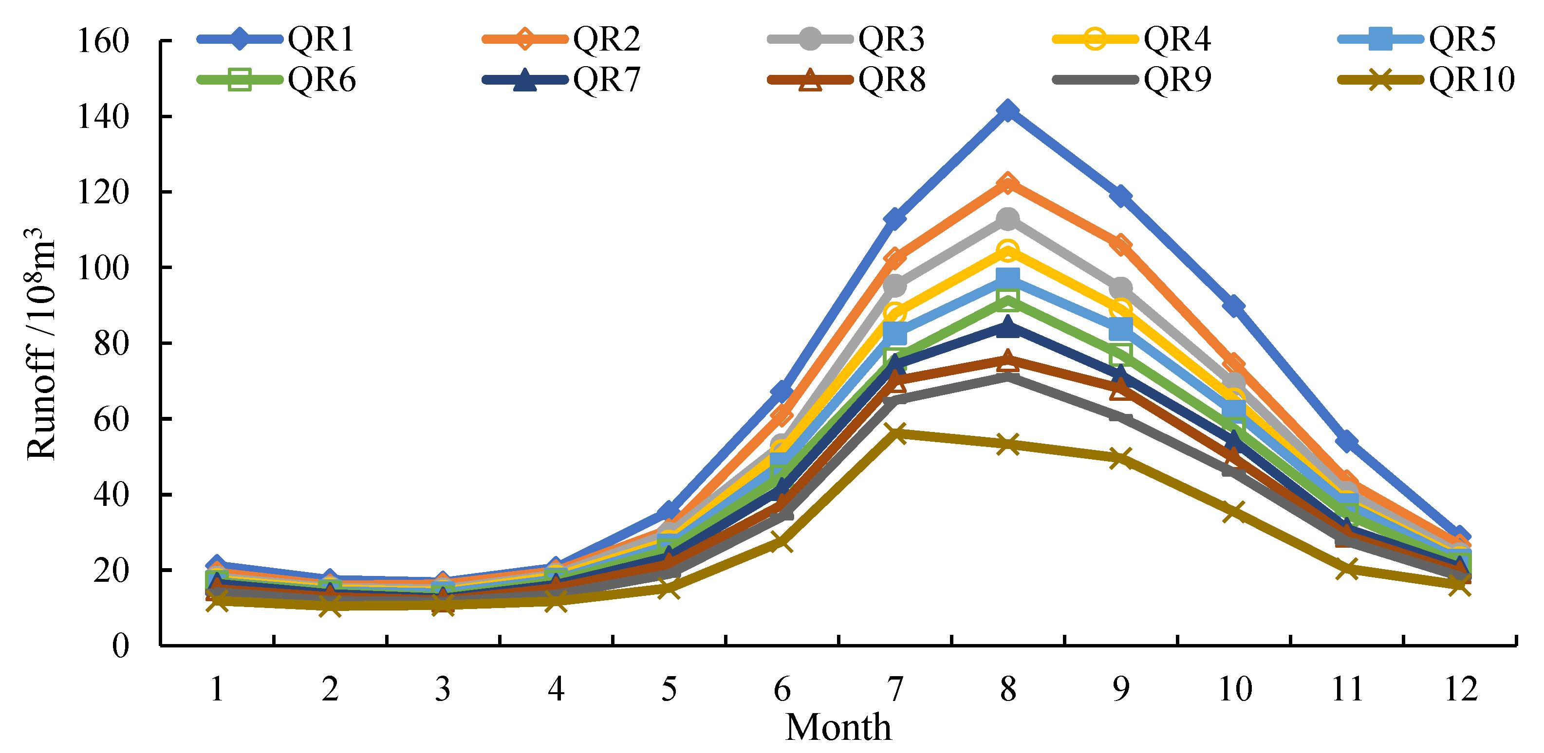
| June | 67.2 | 60.9 | 53.1 | 51.5 | 48.1 | 44.9 | 41.5 | 37.3 | 34.1 | 27.6 |
| July | 112.9 | 102.4 | 95.3 | 88.0 | 82.7 | 75.9 | 74.3 | 70.1 | 64.9 | 56.2 |
| August | 141.6 | 122.4 | 112.9 | 104.5 | 96.9 | 91.4 | 84.6 | 75.6 | 71.2 | 53.3 |
| September | 119.0 | 106.1 | 94.6 | 89.0 | 83.8 | 77.0 | 71.4 | 68.0 | 60.4 | 49.6 |
| October | 89.8 | 74.6 | 69.3 | 65.1 | 62.0 | 57.5 | 54.1 | 49.6 | 45.7 | 35.5 |
| November | 54.1 | 43.6 | 40.4 | 38.1 | 37.3 | 34.7 | 31.0 | 29.2 | 27.6 | 20.4 |
| December | 28.9 | 26.5 | 24.2 | 23.2 | 22.6 | 21.5 | 20.8 | 19.5 | 18.4 | 16.0 |
| January | 21.1 | 19.3 | 18.1 | 17.4 | 16.9 | 16.8 | 16.4 | 15.1 | 14.2 | 12.0 |
| February | 17.4 | 16.0 | 15.4 | 14.9 | 14.5 | 14.2 | 13.7 | 13.0 | 11.9 | 10.5 |
| March | 16.8 | 16.2 | 15.0 | 14.4 | 14.0 | 12.9 | 12.6 | 12.1 | 11.7 | 10.8 |
| April | 20.7 | 19.7 | 18.8 | 18.3 | 17.5 | 17.0 | 16.1 | 15.3 | 13.5 | 11.8 |
| May | 35.5 | 30.7 | 29.7 | 27.6 | 26.5 | 25.3 | 23.5 | 21.6 | 19.0 | 15.3 |
| Month | Representative Runoff QR | |||||||||
|---|---|---|---|---|---|---|---|---|---|---|
| 1 | 2 | 3 | 4 | 5 | 6 | 7 | 8 | 9 | 10 | |
| June | 65.9 | 59.5 | 54.5 | 51.0 | 47.9 | 44.8 | 41.7 | 38.6 | 34.4 | 20.0 |
| July | 108.7 | 99.3 | 92.9 | 87.8 | 83.3 | 79.0 | 75.1 | 70.5 | 64.1 | 39.8 |
| August | 139.0 | 122.4 | 112.7 | 104.9 | 97.7 | 91.1 | 84.7 | 77.7 | 68.7 | 36.2 |
| September | 114.6 | 103.0 | 94.9 | 88.4 | 82.8 | 77.8 | 72.9 | 67.5 | 60.8 | 36.6 |
| October | 83.7 | 75.4 | 70.0 | 65.5 | 61.6 | 57.9 | 54.4 | 50.3 | 45.5 | 28.3 |
| November | 51.4 | 45.5 | 42.1 | 39.1 | 36.7 | 34.4 | 32.0 | 29.4 | 26.4 | 15.9 |
| December | 29.0 | 26.7 | 25.1 | 23.9 | 22.9 | 21.9 | 20.8 | 19.6 | 18.0 | 12.6 |
| January | 20.6 | 19.4 | 18.5 | 17.9 | 17.2 | 16.6 | 16.0 | 15.2 | 14.3 | 10.0 |
| February | 17.3 | 16.3 | 15.6 | 15.0 | 14.5 | 14.0 | 13.5 | 13.0 | 12.2 | 8.4 |
| March | 16.8 | 15.8 | 15.0 | 14.5 | 13.9 | 13.4 | 12.9 | 12.3 | 11.5 | 8.1 |
| April | 21.1 | 19.6 | 18.7 | 17.9 | 17.2 | 16.5 | 15.8 | 15.1 | 14.1 | 9.6 |
| May | 34.9 | 31.6 | 29.5 | 27.8 | 26.2 | 24.8 | 23.4 | 21.7 | 19.6 | 10.2 |
Publisher’s Note: MDPI stays neutral with regard to jurisdictional claims in published maps and institutional affiliations. |
© 2022 by the authors. Licensee MDPI, Basel, Switzerland. This article is an open access article distributed under the terms and conditions of the Creative Commons Attribution (CC BY) license (https://creativecommons.org/licenses/by/4.0/).
Share and Cite
Zhang, H.; Zhang, L.; Chang, J.; Li, Y.; Long, R.; Xing, Z. Study on the Optimal Operation of a Hydropower Plant Group Based on the Stochastic Dynamic Programming with Consideration for Runoff Uncertainty. Water 2022, 14, 220. https://doi.org/10.3390/w14020220
Zhang H, Zhang L, Chang J, Li Y, Long R, Xing Z. Study on the Optimal Operation of a Hydropower Plant Group Based on the Stochastic Dynamic Programming with Consideration for Runoff Uncertainty. Water. 2022; 14(2):220. https://doi.org/10.3390/w14020220
Chicago/Turabian StyleZhang, Hongxue, Lianpeng Zhang, Jianxia Chang, Yunyun Li, Ruihao Long, and Zhenxiang Xing. 2022. "Study on the Optimal Operation of a Hydropower Plant Group Based on the Stochastic Dynamic Programming with Consideration for Runoff Uncertainty" Water 14, no. 2: 220. https://doi.org/10.3390/w14020220