
Stochastic Flood Risk Assessment under Climate Change Scenarios for Toronto, Canada Using CAPRA

1
Department of Civil Engineering, Lassonde School of Engineering, York University, Toronto, ON M3J 1P3, Canada
2
IHE Delft Institute for Water Education, 2611 AX Delft, The Netherlands
3
Department of Civil Engineering, Faculty of Engineering, McMaster University, Hamilton, ON L8S 4K1, Canada
*
Author to whom correspondence should be addressed.
Water 2022, 14(2), 227; https://doi.org/10.3390/w14020227
Submission received: 23 November 2021
/
Revised: 9 January 2022
/
Accepted: 10 January 2022
/
Published: 13 January 2022
(This article belongs to the Special Issue Hydro-Meteorological Hazards under Climate Change)
Abstract
:Amongst all natural disasters, floods have the greatest economic and social impacts worldwide, and their frequency is expected to increase due to climate change. Therefore, improved flood risk assessment is important for implementing flood mitigation measures in urban areas. The increasing need for quantifying the impacts of flooding have resulted in the development of methods for flood risk assessment. The aim of this study was to quantify flood risk under climate change scenarios in the Rockcliffe area within the Humber River watershed in Toronto, Canada, by using the Comprehensive Approach to Probabilistic Risk Assessment (CAPRA) method. CAPRA is a platform for stochastic disaster risk assessment that allows for the characterization of uncertainty in the underlying numerical models. The risk was obtained by integrating the (i) flood hazard, which considered future rainfall based on the Representative Concentration Pathways (RCPs 2.6, 4.5, 6.0, and 8.5) for three time periods (short-term: 2020–2049, medium-term: 2040–2069, and long-term: 2070–2099); (ii) exposed assets within a flood-prone region; (iii) vulnerability functions, which quantified the damage to an asset at different hazard levels. The results revealed that rainfall intensities are likely to increase during the 21st century in the study area, leading to an increase in flood hazards, higher economic costs, and social impacts for the majority of the scenarios. The highest impacts were found for the climate scenario RCP 8.5 for the long-term period and the lowest for RCP 4.5 for the short-term period. The results from this modeling approach can be used for planning purposes in a floodplain management study. The modeling approach identifies critical areas that need to be protected to mitigate future flood risks. Higher resolution climate change and field data are needed to obtain detailed results required for a final design that will mitigate these risks.
Keywords:
flood risk; climate change; exposure; vulnerability; Toronto; stochastic analysis; flood hazard; CAPRA1. Introduction
Amongst all natural disasters, floods have the greatest social and economic impacts worldwide [1]. Globally, flooding-related disasters account for approximately one-third of economic losses and more than half of human fatalities related to all natural disasters [2]. There are different types of floods—river flooding, flash flooding, groundwater flooding, drain and sewer flooding, dam failure, and storm surge [3]. Of these, river flooding is the most expensive and frequent type of flood, affecting most of the countries around the world [4].
In recent decades, flood frequency has increased on a global scale [5]. The main causes of this are the poor management of river basins, deforestation, land-use change, and increased urbanization and economic activities in flood-prone areas. These factors have changed the hydrological regimes of rivers, causing higher rates of runoff. In addition, global climate change is expected to increase extreme weather events and, therefore, increase floods in terms of both the spatial extent and frequency [6]. Global temperature and rainfall intensities have been rising since the 20th century, and higher increases in both parameters are projected to occur by the end of the 21st century. For example, in Ontario, Canada, an increase of 18.4% in the average annual rainfall has been projected between 2013 to 2100 [7]. The increase in flood frequency and related losses have highlighted the urgent need to improve flood risk management.
There is an increasing need to develop and improve methods for flood risk assessment to estimate areas susceptible to flooding and to quantify economic losses and social impacts. The most common, widely used, and most applicable models for river flood risk assessment were reviewed in this study (which are summarized in Table 1). Of the methods reviewed, many of the methods, including Flood Loss Estimation Model (FLEMO) [8], FloodCalc [9,10], the In-depth Synthetic Model for Flood Damage Estimation (INSYDE) [11], Strategies of Urban Flood Risk Management (SUFRI) [12], RiskScape [13], LATIS [14], and Hydrologic Engineering Center Flood Impact Analysis (HEC-FIA) [15], amongst others, do not have the capability for hydrological and hydraulic modeling to inform the flood risk analysis. Instead, these methods rely on user-inputted flood depths, duration, or inundation maps, which means that these methods have limitations in terms of characterizing the spatial and temporal trends of flood hazards and risks. Furthermore, most of the methods listed in Table 1 are deterministic and, therefore, do not account for the uncertainty associated with flood hazards and the associated economic damages. Lastly, the social impacts of floods are not widely considered in these methods, with only FloodCalc [9,10], SUFRI [12], RiskScape [13], LATIS [14], HEC-FIA [15], Hazus-MH [16], and CAPRA [17] considering social impacts, which are typically limited to fatalities rather than other direct, intangible social impacts. Thus, one of the major limitations and drawbacks found among these methods is that the social risk has been evaluated much less frequently than the economic risk (67% of the methods reviewed do not account for the social impacts of floods). In addition, half of the methods only perform deterministic risk, and only 44% of the methods developed software for flood risk, from which only three are open source (Multicriteria Approach, Kalypso, and CAPRA). Therefore, there is a need to develop and test the use of flood risk assessment methods that can characterize the uncertainty of flood risk (using stochastic methods) and account for both the social and economic impacts of floods. This review of the literature demonstrates the major limitations of current flood risk methods. Furthermore, it is important to consider the effects of future climate change, as general circulation model (GCM) models have predicted an increase in rainfall intensities in the future, which may lead to an increase in flood risk, along with future changes to land use and population growth.
The CAPRA method for flood risk assessment [28,29,30,31] was chosen in this study due to its advantages over the other methods. It allows for both deterministic and stochastic risk assessment through the generation of stochastic rainfall scenarios (the only model to do so of the 18 models reviewed). In addition to quantifying economic damages, it also quantifies the social impacts of floods and the spatial distribution of flood risk. It has an open-source group of programs that focus on hazard, vulnerability, and risk assessment. CAPRA was developed by Ingeniar, Evaluación de Riesgos Naturales (ERN), Ingenieria Tecnica Y Cientifica (ITEC), and the International Centre for Numerical Methods in Engineering (CIMNE). Several risk assessment studies focusing on different types of hazards have used CAPRA. A study in Barcelona, Spain used CAPRA for a probabilistic earthquake risk assessment and a holistic evaluation of risk by considering the lack of resilience and the socioeconomic fragility [30]. The CAPRA method was also applied to Acapulco city, Mexico, to perform a probabilistic flood risk assessment [31]. A study used CAPRA to evaluate the probabilistic hurricane risk in Guatemala and considered the effects of climate change [32]. CAPRA was used to evaluate seismic risk, tropical cyclone risk, and flooding risk at a global scale for GAR15 [33]. CAPRA has been widely used across the world over the last 10 years and a summary of its applications has been presented by Reinoso et al. [34].
Objectives
In 2015, the National Disaster Mitigation Program (NDMP) was created to mitigate the impacts of natural disasters in Canada. In 2018, the Toronto Region Conservation Authority (TRCA) started the Flood Risk Assessment and Ranking project [35], which was the final stage of the NDMP. The scope of this project was to quantify the risk associated with riverine flooding at each of the 43 flood-vulnerable clusters within the TRCA’s jurisdiction in the City of Toronto, and to rank these clusters relative to each other. The Rockcliffe area was amongst the top ten clusters with the highest susceptibility to flooding. A flood risk assessment for the Rockcliffe area was conducted by the TRCA as part of the Flood Risk Assessment and Ranking project. However, their approach only included steady-state hydraulic modeling for current climate conditions using deterministic rainfall as the input and did not consider the social impacts of flooding.
Therefore, the objective of this study was to expand on previous risk assessment efforts for the Rockcliffe area using the CAPRA method to quantify the flood risk (including economic and social damages) using stochastic rainfall scenarios for both historical and future projections of rainfall. By using unsteady-state flow to account for the temporal variability of surface runoff and by driving the hydraulic models by using future climate conditions, the results of this study will allow the TRCA to provide a higher level of service in flood hazard forecasting and risk analysis. Note that the future changes to land use and population density are outside of the scope of this study. Previously developed hydrological and hydraulic models, as well as estimates for economic and social damages within the region, were used within the CAPRA framework for this study. The future rainfall scenarios are based on the different climate scenarios (Representative Concentration Pathways (RCPs) 2.6, 4.5, 6.0, and 8.5) for three time periods (short-term: 2020–2049, medium-term: 2040–2069, and long-term: 2070–2099). Therefore, the contributions of this study provide estimates of flood risk (including both economic and social impacts) for the Rockcliffe region for historical and future climate conditions using a stochastic framework developed with CAPRA, which allows for the quantification of uncertainty in risk estimates. The study integrates the key components of flood risk, including hazard, exposure, and vulnerability, the latter of which has been ignored in previous efforts for the region. Doing so highlights and improves our understanding of how climate change will change rainfall regimes in the area as well as its effects on flood hazards and the economic and social consequences of floods. The stochastic approach proposed herein provides risk results for a wide range of possible scenarios, the likelihood of occurrences, and the quantification of expected losses and damages. This will help provide information that can guide future flood mitigation efforts in the region. Details of the study area and the models used, as well as the risk assessment framework, are detailed in Section 2, followed by the results and discussion in Section 3, and conclusions and recommendations for future research in Section 4.
2. Materials and Methods
2.1. Study Area
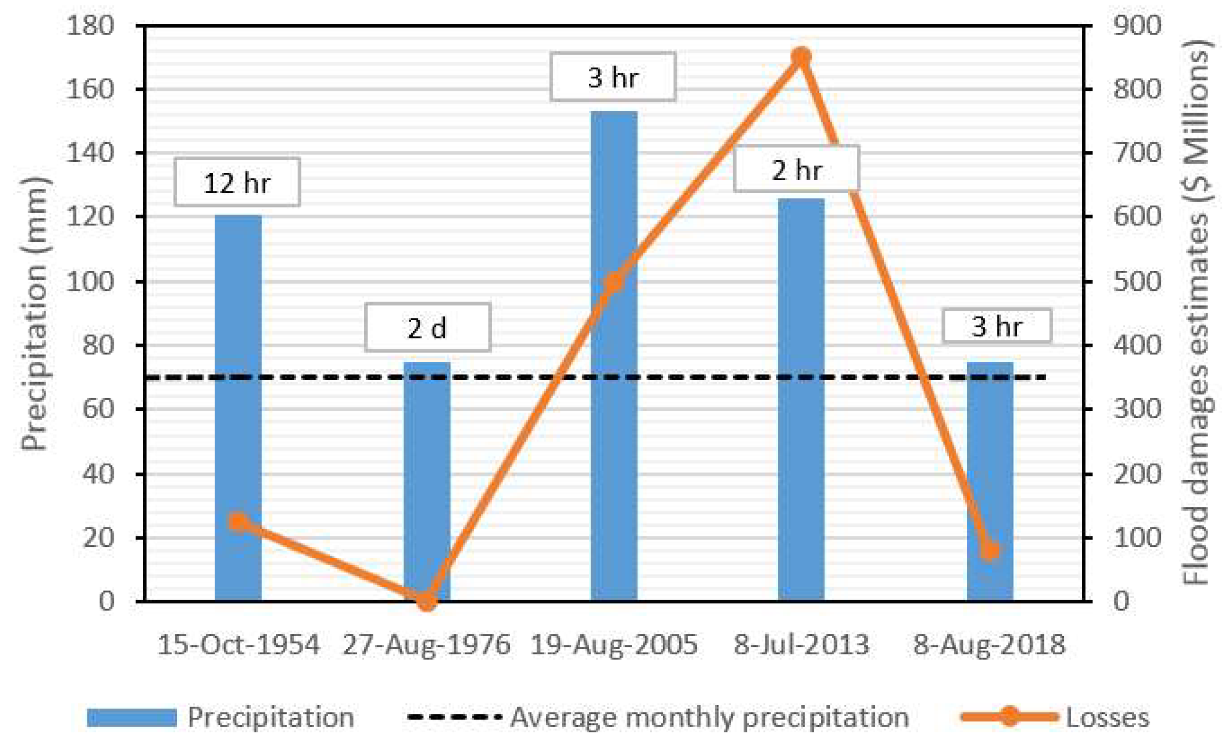
Toronto, located in Southern Ontario, is the most populous city in Canada. Over the past century, five major flood events in Toronto have resulted in significant environmental, economic, and social damages. Figure 1 shows the rainfall intensities of these events, represented in blue bars, along with its corresponding economic losses, shown with an orange line. It also shows the average monthly rainfall (around 70 mm) as a dashed black line. It is clear from the chart that these five events had significant rainfall intensities and the rainfall depths exceeded the average monthly rainfall. The reasons for the high susceptibility to floods in Toronto include the increase in impervious areas due to urbanization, tributaries of the lower Don River have been filled or artificially channelized, wetlands have been filled or drained, the characteristics of the river valley, which is a non-confining valley, and the smooth topography of Toronto [36].
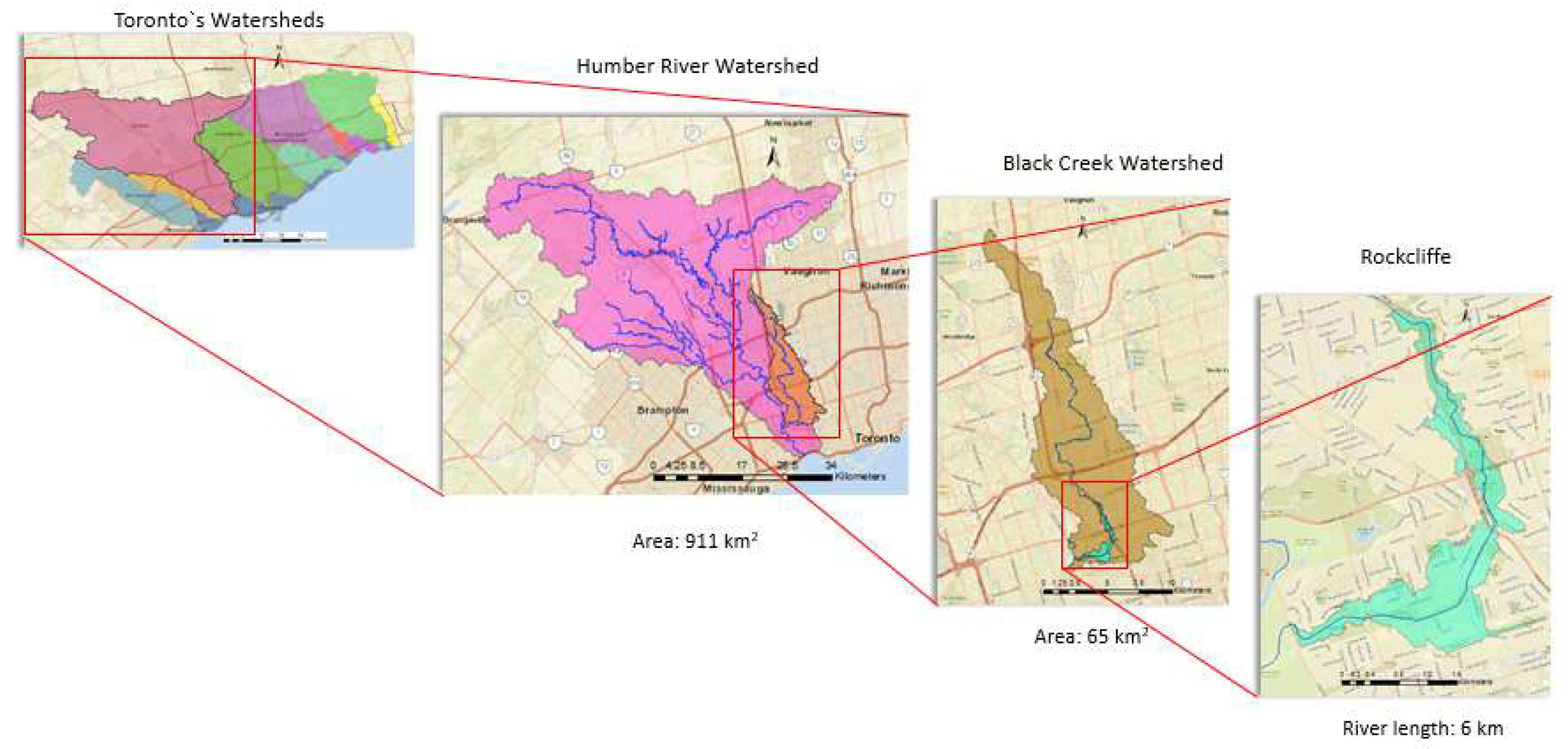
There are eleven watersheds within Toronto. The Humber River watershed is the largest with an area greater than 911 km2 and a population greater than 850,000 inhabitants. Most of the southern parts of the Humber River watershed have been highly urbanized. The Black Creek subwatershed is part of the Humber River watershed and has a drainage area of 65 km2. The Black Creek is located at the east of the Humber River and the junction of these rivers is at Dundas Street. This area is highly susceptible to flooding, as it is completely urbanized and has a limited flow capacity for heavy storms, resulting in floods. Based on daily discharge data for the year 2020 [37], the average flow at the Black Creek near Weston hydrometric station (station number 02HC027) was 0.80 m3/s, and the maximum and minimum daily flows were 18.9 m3/s and 0.11 m3/s, respectively. For the period from 1966 to 2020, the mean daily flow was 0.72 m3/s, and the maximum observed discharge occurred in July 2013, with a peak flow of 41.4 m3/s. There are different land uses in this area, such as industrial, commercial, institutional, and residential. In addition, the creek has been highly modified with artificial concrete channels and several bridges and culvert crossings. The watercourse’s floodplain has been encroached, which has increased the flood risk in this area. Furthermore, the maximum flow capacity of the low flow concrete channel in this area is only a 10-year storm [38]. It is a narrow corridor that is, on average, 15 m wide and 2 m deep. The Rockcliffe region was selected as the case study to apply and test the proposed method due to previous flooding issues in the region. It is located downstream end of the Black Creek, a subwatershed of the Humber River watershed in Toronto, Canada (as illustrated in Figure 2).
2.2. Overview of the Proposed Modeling Methodology
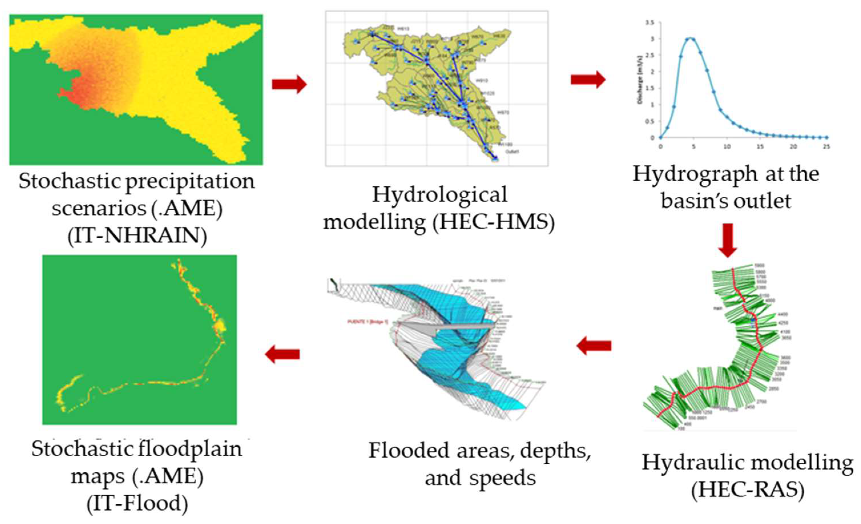
In this study, we quantified the flood risk for the Rockcliffe region using the CAPRA method. This stochastic framework considers the frequencies of extreme rainfall events and generates stochastic rainfall scenarios with random shapes, locations, and rainfall intensities based on observed data. The CAPRA platform contains four submodules—(i) IT-NHRain, which evaluates the stochastic rainfall hazard by creating stochastic scenarios of rainfall intensity; (ii) IT-Flood, which uses the stochastic rainfall scenarios to generate multiple flood scenarios by using a hydrological (HEC-HMS) and hydraulic model (HEC-RAS); (iii) Funciones de Vulnerabilidad (FUNVUL) Simplified creates vulnerability functions (depth–damage curves) to estimate the economic costs of each flood scenario; finally, (iv) the overall flood risk is calculated on CAPRA-GIS software by integrating the flood hazard with the vulnerability of exposed elements. The following sections describe each of these processes in detail.
2.3. Rainfall Hazard Analysis
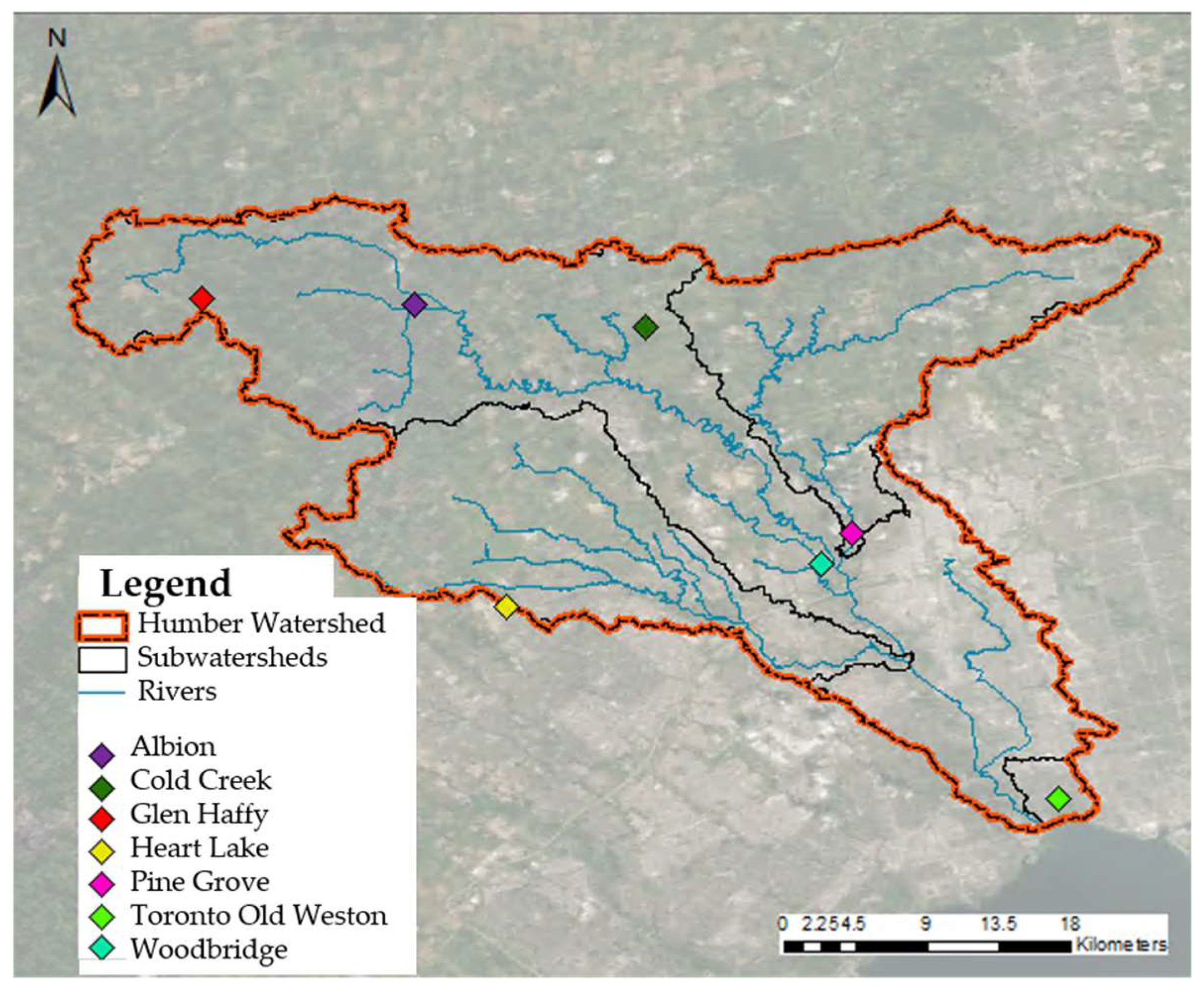
The rainfall hazard analysis was performed for both current and future climate conditions. The current climate conditions were based on daily observed rainfall data for 30 years of records (1960 to 1989) obtained from seven rain gauges within the Humber River watershed (the locations are shown in Figure 3). These historical daily rainfall data were obtained from Environment Canada. To account for future climate conditions, future daily rainfall data were obtained from the Ontario Climate Data Portal (OCDP) which contains climate projections in Ontario from various General Circulation Models (GCMs) [7]. The data portal provides climatic scenarios of the Intergovernmental Panel on Climate Change (IPCC) Fifth Assessment Report on Climate Change (AR5) for different RCPs [39]. In this study, projections from RCPs 2.6, 4.5, 6.0, and 8.5 were used, where RCP 2.6 is the most optimistic scenario, as it projects the lowest CO2 concentration, and RCP 8.5 is the most pessimistic with the highest CO2 concentration [40]. In addition, projections for three future time periods, short- (2020–2049), medium- (2040–2069), and long-term (2070–2099), were used for the analyses.
There are several GCMs available in the OCDP, including NorESM1-M, MRI-CGCM3, MPI-ESM-MR, MIROC-ESM, and IPSL-CM5A-MR, among others. To determine the models that best represent the climate of the study area, the simulated historical GCM results were compared to the observed historical monthly rainfall using the Pearson correlation coefficient. The GCMs that provided the highest correlation between these two datasets (simulated and observed monthly rainfall) were selected for the analyses. For the climate scenarios RCPs 2.6, 4.5, and 6.0, the NorESM1-M model was selected. For RCP 8.5, the CMCC-CEM model was chosen. The next step was to downscale the GCM output using the Delta Change method, where the change factor is calculated through the ratio of the mean future (simulated) monthly rainfall and the mean historical (simulated) monthly rainfall [41]. The future downscales rainfall values were then obtained by multiplying the observed rainfall by the calculated change factor.
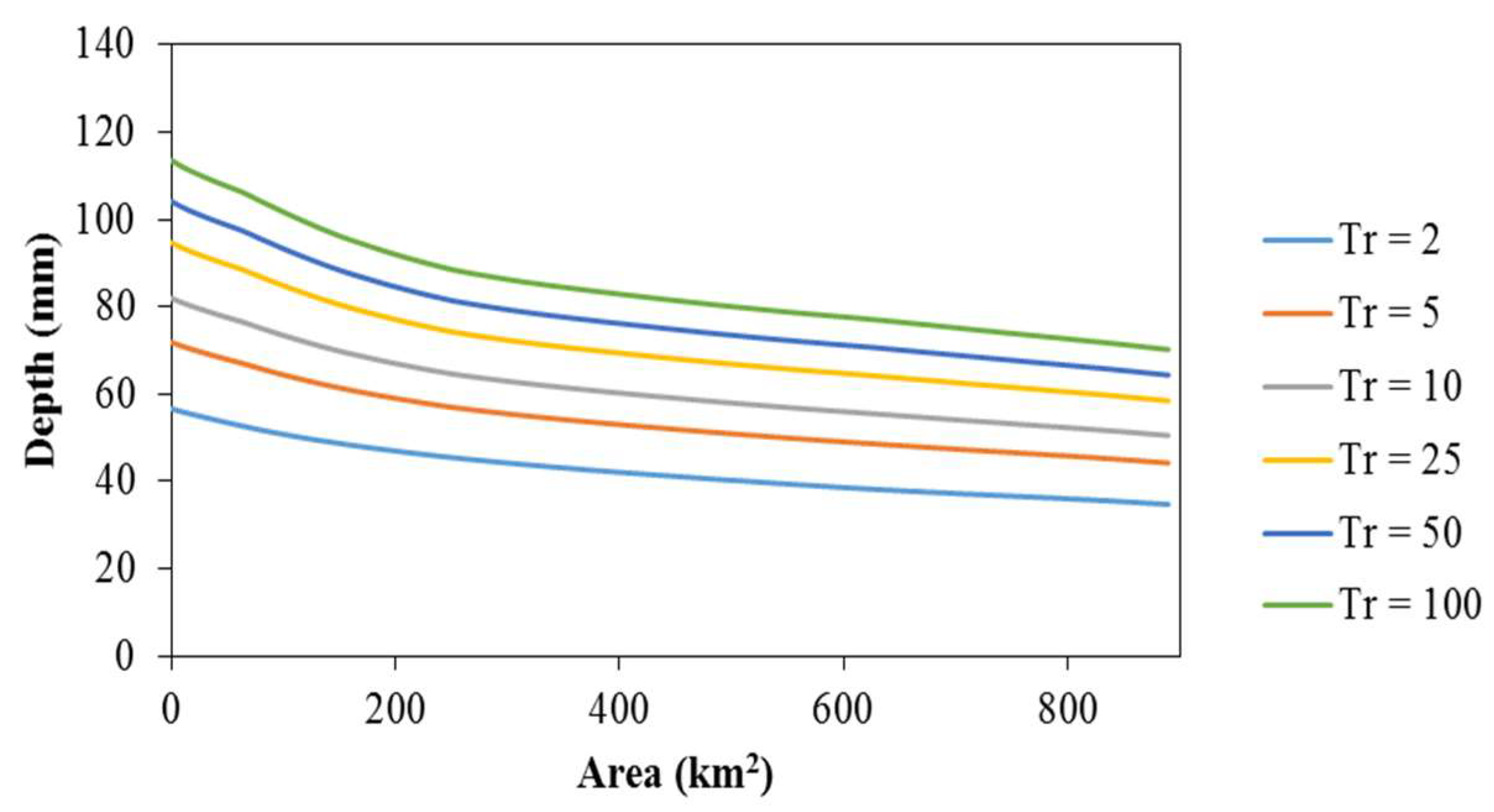
The observed and projected downscaled rainfall data were then used to generate stochastic rainfall scenarios with a random shape, location, and rainfall intensities for a given duration and frequency. The CAPRA method includes the following steps to create stochastic rainfall scenarios. The first step was to conduct a geomorphological analysis of the basin and stream to determine the area of influence, which corresponds to the potentially flooded area and watershed. Following this, a hydrological characterization of the basin was performed to determine the maximum rainfall spatial extent, and to identify the preferential storm centers for the observed and simulated rainfall data. The maximum rainfall spatial extent analysis consists of the generation of Depth–Area–Duration–Frequency (DADF) curves. These curves establish the relationship between the maximum depth of average rainfall (D), the area (A) over which this rainfall falls, the duration (D) during which the rainfall takes place, and the frequency (F) of the events for each depth, spatial coverage, and duration. DADF curves determine the maximum rainfall for different durations and frequencies over a range of areas and describe the rainfall pattern of the basin. In order to obtain DADF curves, first, the depth–area–duration (DAD) curves were built (one for each event and duration). Then the frequency (return period) was calculated for each rainfall depth for a certain area and duration, established in the DAD curves, which results in DADF curves for the homogeneous hydrological zone. For the frequency analysis, the Gumbel distribution was used using the probability-weighted moments method for estimating the parameters of the probability function [42]. The frequency analysis was performed for six return periods (2, 5, 10, 25, 50, and 100 years). The duration of the storms for the DADF curves is one day. Figure 4 shows an example of the DADF curves generated for the historic period (1960–1989).
In order to identify the preferential storm centers, isohyet maps were generated and the zones with higher rainfall intensities were identified. Finally, the stochastic storms are generated from the information within the DADF curves and the isohyet maps, which determine the typical patterns and preferential location of storms in the study area. Thirty stochastic scenarios for each return period were generated with a grid size of 500 m for the rainfall maps.
2.4. Flood Hazard Analysis
Flood hazard is defined by the relationship between flood depth and its probability of occurrence, which is represented by depth–frequency curves [16], and by flood hazard maps, which determine the spatial extent of flooded areas based on the estimated discharges for different return periods.
For the flood hazard analysis, stochastic rainfall events, described in Section 2.3, were used to run a hydrological model, which provides the runoff hydrograph for the basin analyzed based on the rainfall. This hydrograph is then fed into the hydraulic model as an upstream boundary condition, which routes the hydrograph through the main channel (i.e., the Humber River) and, thus, water (or flood) levels and velocities can be obtained for the area of interest. These parameters are then used to generate the corresponding floodplain maps, which show the flood extent and water depth (velocities were not used in this study for the flood risk analysis).
Since the stochastic rainfall scenarios only provide the rainfall intensity and its spatial distribution, the Atmospheric Environment Service—Southern Ontario (AES-SO) design storm was used to define the temporal distribution of the storm events [43]. A calibrated hydrological model of the Humber River was provided by the TRCA in the software Visual OTTHYMO (VO) [44] and was used as a reference to create the hydrological model in HEC-HMS Version 4.0, as CAPRA requires this specific software for the hazard module. To create the hydrological model, the subbasins, reaches, junctions, and the outlet were created in the Hydrologic Engineering Center’s Geospatial Hydrologic Modeling (HEC-GeoHMS) extension of ArcGIS from the DEM, with a ground resolution of 5 m x 5 m (obtained from Scholars GeoPortal). For the subbasin elements, the loss method used was the SCS Curve Number and the transform method selected was the SCS Unit Hydrograph. The canopy, surface, and baseflow components were not considered. For the reach elements, the routing method selected was Muskingum–Cunge, and the gain/loss component was not included. As for the meteorological model, only the precipitation was taken into account by using the gridded precipitation method. The model was calibrated by comparing the results of the HEC-HMS model to the OTTHYMO (VO) model provided by the TRCA by using the univariate gradient method and the peak-weighted Root Mean Square Error as the objective function. The difference in peak flow between the two models for the 2-year, 24-h AES-SO design event was 1.3%, which was considered to be suitable for this study.
The 1D hydraulic model was developed in HEC-RAS Version 4.1 for the Black Creek within the Rockcliffe region, which was run under unsteady flow conditions using the hydrograph from the HEC-HMS model. Note that the version of CAPRA used for this study only allows for the use of a 1D hydraulic model (HEC-RAS Version 4.1). One-dimensional models assume that water flows unidirectionally (longitudinally) in the main channel. However, the secondary flows perpendicular to the main channel that occur during flood events (as a result of the spills) cannot be modeled in 1D [45]. Two-dimensional models may be capable of modeling these secondary flows and are better for modeling flows through hydraulic structures, confluences of streams, and compound channels, among others. However, for a general analysis of floodplains, as presented in this study, 1D modeling is sufficient, but specific adaption and risk measures should be modeled using 2D hydraulic models.
The original, calibrated HEC-RAS hydraulic model was provided by the TRCA, which used bathymetric data to create the model. However, this model was unstable to perform unsteady state simulations as required for this study. Thus, a Digital Elevation Model (DEM) with a ground resolution of 5 m was used to create a new HEC-RAS model using HEC-GeoRAS. This model used the same model parameters as the original TRCA model. The upstream boundary condition was defined by the flow hydrograph (from HEC-HMS), and the downstream boundary was the normal depth. The model was calibrated by comparing the results to the TRCA model for steady-state conditions. Note that for the study area, the highest available resolution for the DEM was 5 m—this can affect the accuracy of the cross-sections of the river in the hydraulic model. However, the simulated flows were compared with observed flows from a flow gauge and there were no significant differences.
The IT-Flood module within CAPRA integrates the hydrological and hydraulic models, along with the set of stochastic rainfall scenarios, to generate the flood hazard maps for the corresponding rainfall scenarios. Figure 5 shows a schematic of each step of this analysis. The rainfall and flood hazard scenarios were stored in AME filetypes, which is a collection of raster files (the standard format of CAPRA for hazards) and then used for the hazard analysis. An * AME file is a raster geodatabase containing a raster for each simulation. The metadata stores additional information, such as the associated frequency of each scenario and the type of evaluated hazard, among others.
2.5. Exposure Assessment
Exposure refers to the elements or assets exposed to a hazard, whether they are buildings, infrastructure, agricultural areas, or people. The exposure of buildings normally includes the type of building, location, the value of assets, and the number of stories (i.e., levels) of the building. The exposure to people includes the population density at a particular location. The vulnerability analysis quantifies the level of damage of a component (typically as a percentage of the exposed value) for a given hazard intensity (e.g., water depth), through vulnerability functions represented as depth–damage curves.
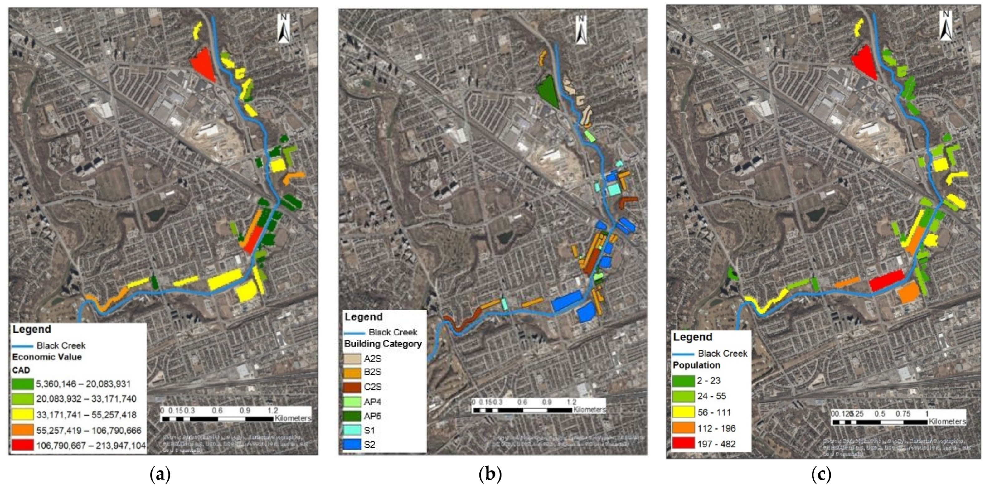
An inventory of the “exposed components” must be quantified to determine the flood risk. These components are the structures or elements that are exposed to flood hazards for a given rainfall event. The exposure was created in ArcMap (as a polygon shapefile) containing the economic value, the building category, and population (which is an indicator of social impact). The polygons of each building category were created using Google Maps. Figure 6 shows the exposure maps for these three categories for the study area. A description of how these categories were quantified follows.
The economic value estimates the economic damages of the exposed components during flood events—this is often a difficult task [46] due to the lack of detailed data. Economic damages are commonly represented through the exceedance probability curve, which describes the probability that the loss will exceed a specific value within a period of time (usually annually), and through the expected annual damage, which is the area under the exceedance probability curve. These damages can be direct, indirect, tangible, or intangible. Direct damages refer to those resulting from direct contact with the hazard (e.g., the damage occurs within a flooded area), whereas indirect damages may result after a delay or outside a flooded area (indirect contact with the hazard). Tangible damages are those that have a specific monetary value, whereas intangible damages are difficult to assess in monetary terms. [46,47,48,49]. In this study, only direct tangible damages were taken into account, which is the most common type of economic flood damage assessment. In the context of flooding, this refers to the physical losses due to the contact with water (i.e., direct) and can be measured based on a monetary value (i.e., tangible), such as the cost of repair or replacement of the assets affected.
The direct damages were based only on the construction value per square meter obtained from the TRCA. The value of contents was not included. Table 2 shows the economic values used for each building category. For consistency, the economic values for the residential buildings were all assigned the same value of the category “House Class A—two floors” or A2S.
Social damages due to flooding include loss of human life, loss of property, loss of livelihoods, mass migration, diseases, disruption of utility services, psychosocial effects, loss of trust in the authorities, and hindering of economic growth and development, amongst others [50]. The social impact was determined by the number of people affected (i.e., exposed) to a flood event. In this study, social impact was limited to tangible damages rather than intangible social effects, such as stress, psychological trauma, or illness [47,48], and as such, is a simplification of the real damages. The population per polygon was calculated based on the area of the polygon and the population density, which was obtained from the 2006 census data for Toronto [51]. In this study, it was assumed that the exposure stays constant with time (i.e., does not change for the future periods). Table 3 summarizes the exposure for the study area, for each building category, the exposed area in m2, the exposed value in Canadian dollars ($), and the exposed population.
2.6. Vulnerability Assessment
Vulnerability is defined as the inherent susceptibility of an element to be affected by a hazard and is directly associated with the element’s exposure to the hazard and inversely proportional to the resistance of the element to cope with it. This means that when a hazard occurs, the vulnerability of the people and the exposed assets will determine the damages caused by the hazard [52]. Vulnerability functions quantify the level of damage of a component for a given hazard intensity. In this study, the hazard intensity is based only on the flood depth (i.e., depth–damage curves).
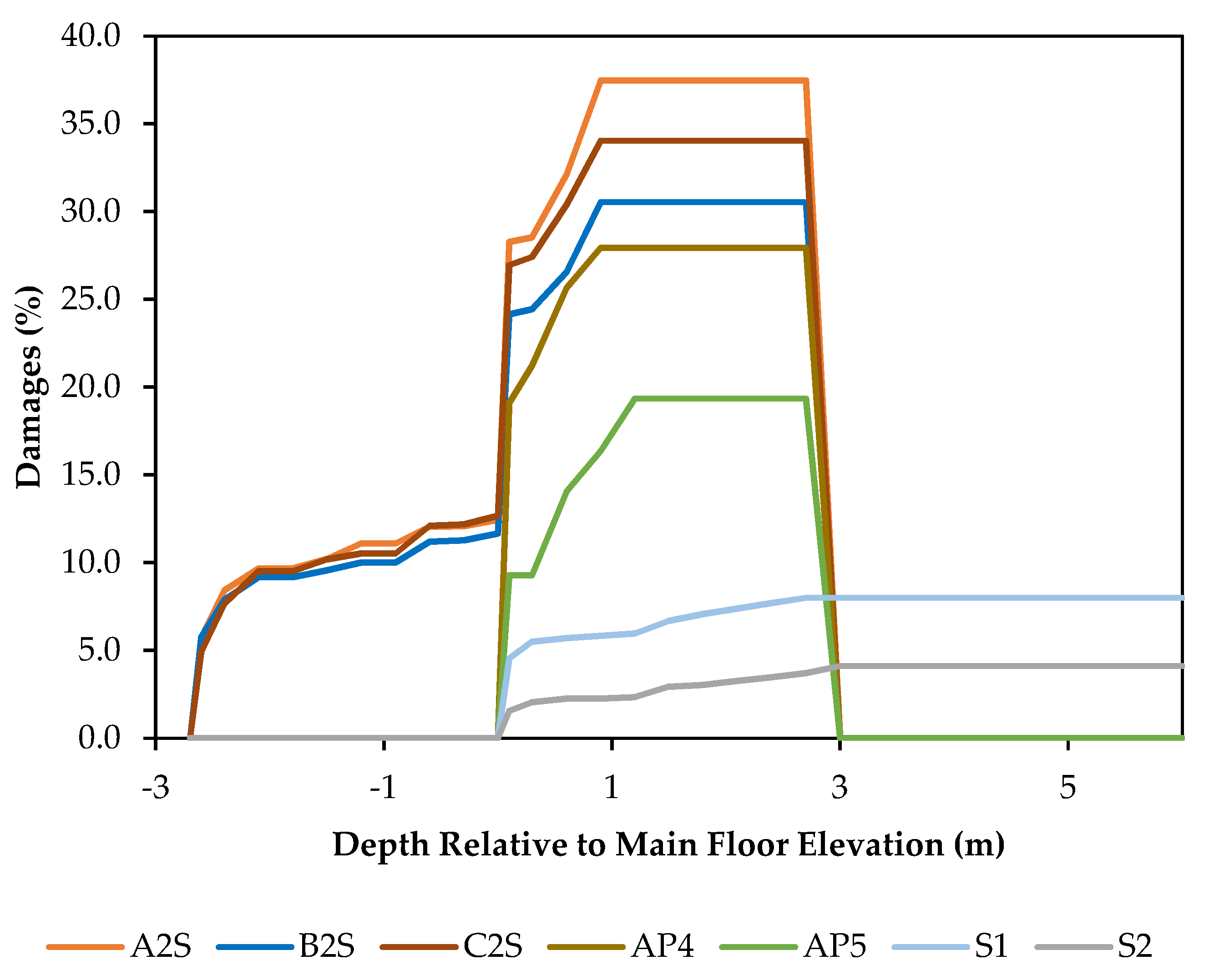
The vulnerability of infrastructure was based on the flood vulnerability functions produced for Alberta [53]. These functions contain depth–damage curves in terms of monetary damage per meter square ($/m2) for the different types of residential and non-residential buildings. The monetary damages of these curves were then transformed to percentages based on the economic values from Table 1. Figure 7 shows the values of the depth–damage curves per building category.
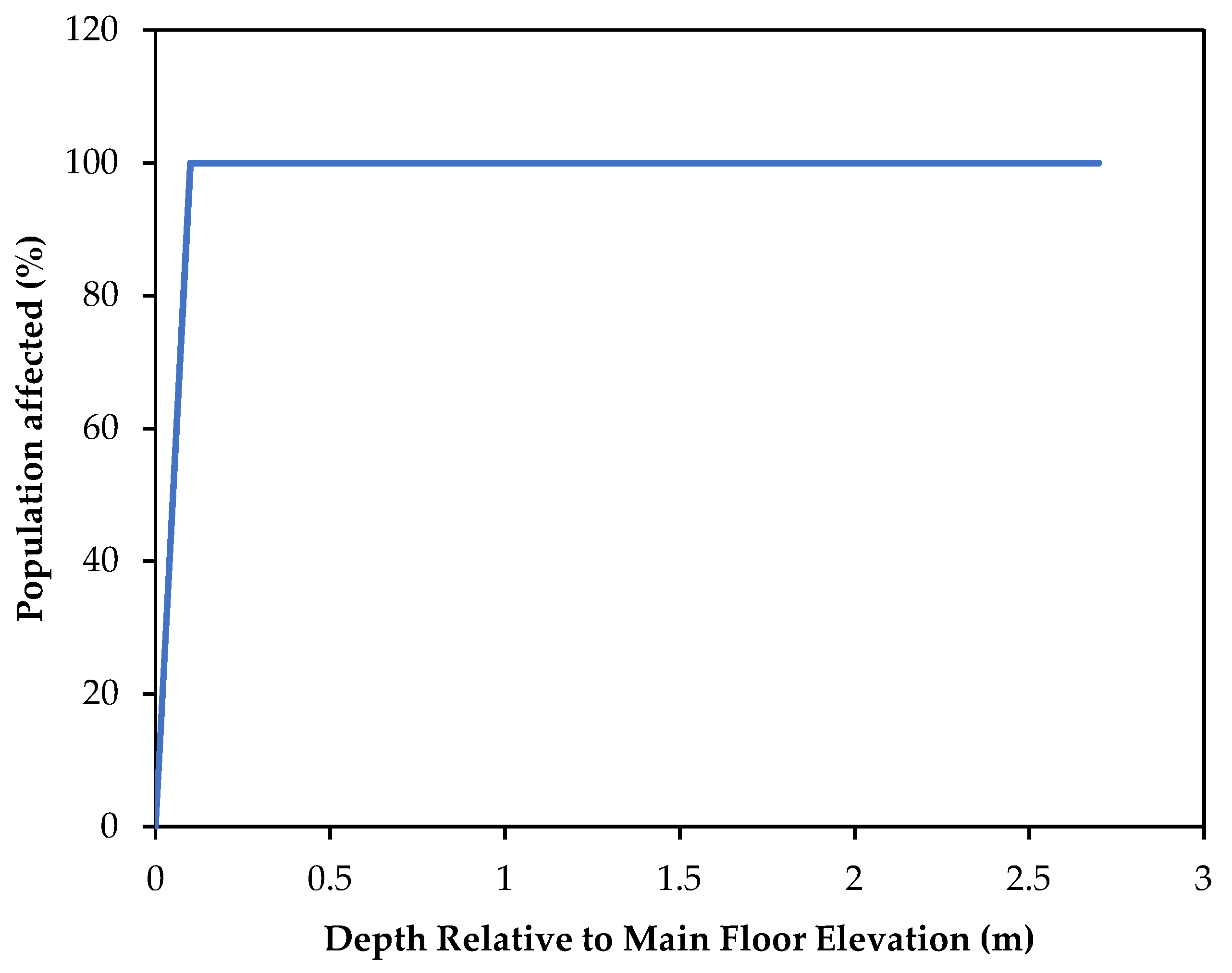
Social vulnerability to flooding disasters has been used by several flooding studies, where the vulnerability is a function of the demographic characteristics, socioeconomic status, land tenure, and neighboring characteristics [54,55]. In this study, a simpler approach was used where the social vulnerability is only a function of the number of people, regardless of their characteristics. As the damages to infrastructure start at a water depth of 0.1 m (from the main floor), it was assumed that people are affected by flooding from a flood depth of 0.1 m. Therefore, for water depths less than 0.1 m, the population affected is 0% and for water depths equal to or higher than 0.1, it is 100%, as shown in Figure 8. The values of the depth–damage curves were inputted into FUNVUL Simplified (the vulnerability module of the CAPRA platform) to create the vulnerability functions in a FVU filetype. FUNVUL Simplified uses equations to calculate the loss mean and the loss standard deviation that corresponds to the mean damage ratio and its corresponding variance [56].
2.7. Flood Risk Analysis
Flood risk refers to the expected losses of a particular hazard (e.g., flood hazard) to a specific element at risk, in a particular time period or scenario [57]. Generally, flood risk is defined as the product of the hazard, exposure, and vulnerability. As the exposure and vulnerability are implicitly evaluated as the consequences of the flood hazard, a simpler definition of flood risk is the product of the probability and the consequences [58]. The risk is developed by associating the hazard on the inventory of exposed assets through the related vulnerability functions, resulting in the quantification of damages, both economic and social.
The final component of the study was the flood risk analysis, which combined the results of the rainfall and flood hazard analyses with the exposure and vulnerability assessment, within a stochastic framework. This component provides the damages (in terms of losses) expected from each stochastic rainfall event and was performed using the CAPRA-GIS module. This software integrates hazard with the vulnerability of exposed elements to generate the flood risk, either for a single scenario (deterministic) or for all scenarios (stochastic). The results are given in a RES filetype, which shows the number of people affected and economic damages (in terms of loss exceedance curve, average annual loss, and probable maximum loss).
The loss exceedance curve, also known as the exceedance rate of loss, represents the frequencies, usually annually, with which events will occur, and within which a specified value of losses is exceeded. The exceedance rate of loss v(p) is calculated with the following equation [17]:
where is the probability that the loss is greater than p given that event i took place, and is the annual occurrence frequency of event i. The probability that the loss is greater than p given that event i took place is computed through vulnerability functions by using the following equation [17]:
where is the probability that the loss exceeds the p-value since the local intensity was I; this term takes into account the uncertainty in vulnerability relationships. is the probability density function of intensity conditioned on the occurrence of the event; this term takes into account the fact that since an event occurred, the intensity at the site of interest is uncertain. The average annual loss is the expected loss per year. It can be obtained by integrating v(p) or by the following equation [17]:
where AAL is the average annual expected loss, is the expected loss value since event i occurred, which depends on the vulnerability of the exposed element, and is the annual occurrence frequency of event i. The probable maximum loss is a measurement of the magnitude of maximum losses that could be expected during the occurrence of a hazard event for a certain return period. In CAPRA-GIS, the probable maximum losses are calculated by using a Beta distribution to find the cumulative probability of each stochastic scenario [17].
3. Results and Discussion
3.1. Climate Change Rainfall Projections
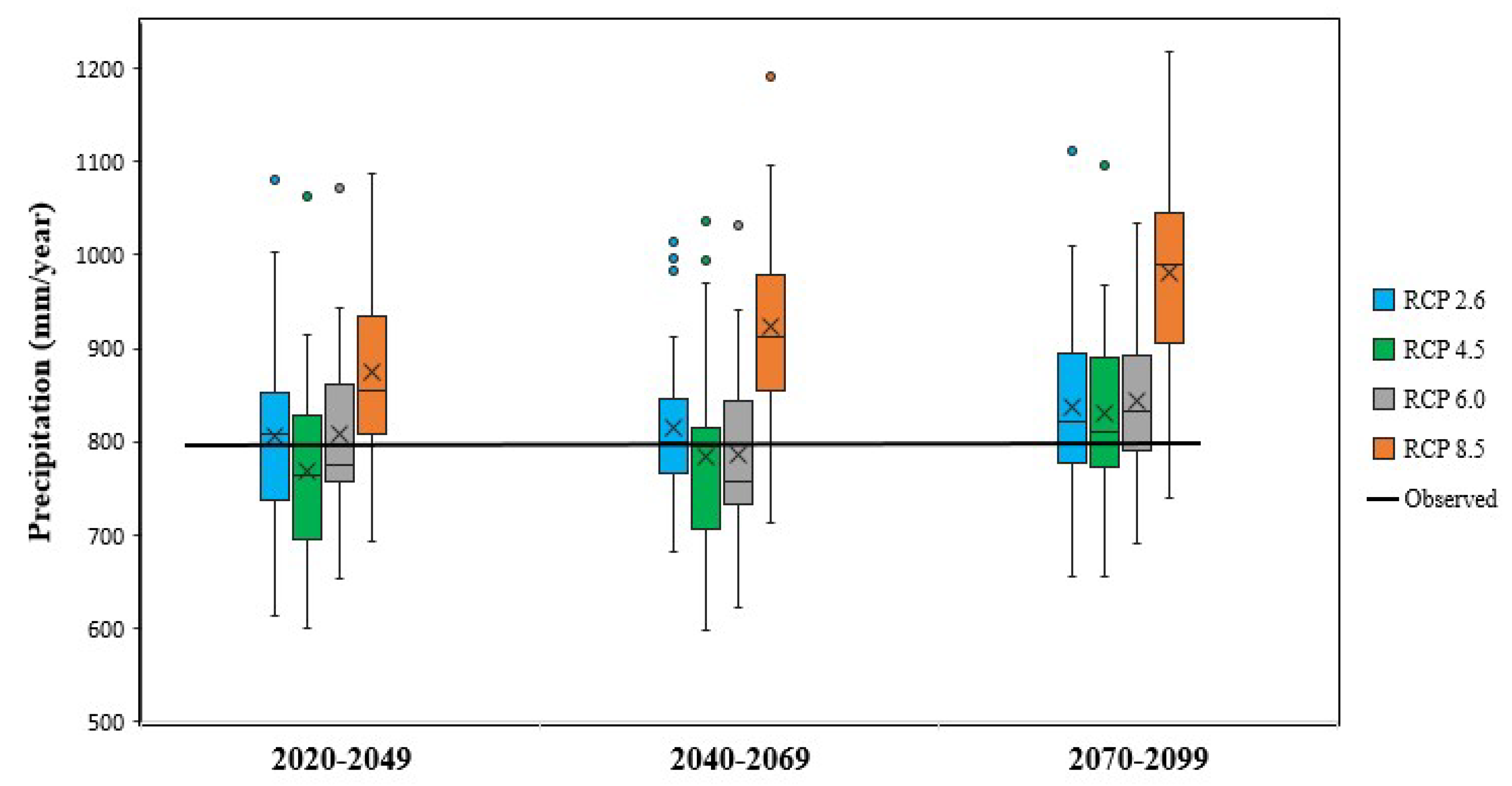
Figure 9 shows a comparison of the historical annual rainfall and projected rainfall in the study area for the three future periods for each of the four climate change RCP scenarios. The climatic scenario RCP 8.5 shows the highest annual rainfall throughout the century with an upper trend, rising from the third quartile (Q3) of rainfall of around 940 mm/year for the short-term period to 980 mm/year in the medium-term period and, finally, to 1300 mm/year in the long-term period. The climatic scenarios RCP 2.6 and RCP 6.0 show similar values in Q3, where the highest values are in the long-term period at around 900 mm/year (RCP 2.6 being slightly higher), followed by the short-term period with approximately 850 mm/year (RCP 6.0 being slightly higher), and the lowest values for both climatic scenarios are presented in the middle-term with around 840 mm/year. The climatic scenario RCP 4.5 shows the lowest rainfall, with the highest values of Q3 in the long-term, at close to 980 mm/year, followed by the short-term period with 830 mm/year and the medium-term with 820 mm/year. On a seasonal basis, historical observations show that the summer season had the highest rainfall while the winter was drier. However, future rainfall trends show that December to May will be wetter, whereas the summer months (June, July, August), October, and February will be drier.
Overall, the climatic scenario RCP 8.5 shows the highest annual rainfall and RCP 4.5 the lowest. The long-term period has the highest annual rainfall values for all the climatic scenarios and the medium-term the lowest (except for the climatic scenario RCP 8.5, the lowest values of which are for the short-term period). In terms of the median, or the second quartile (Q2), almost all are greater than the historical mean, except for RCP 4.5 and RCP 6.0 for both the short and medium-term periods, which are lower. The first quartile (Q1) off all climatic scenarios is below the historical average, except for the climatic scenario RCP 8.5, for which Q1 values for the three periods are all above the observed rainfall. The long-term period projections suggest an increase in annual rainfall for the study area for all RCP scenarios. As mentioned in Section 2.3, these projected rainfalls were first obtained from the OCDP [7] and then downscaled using the Delta Change method.
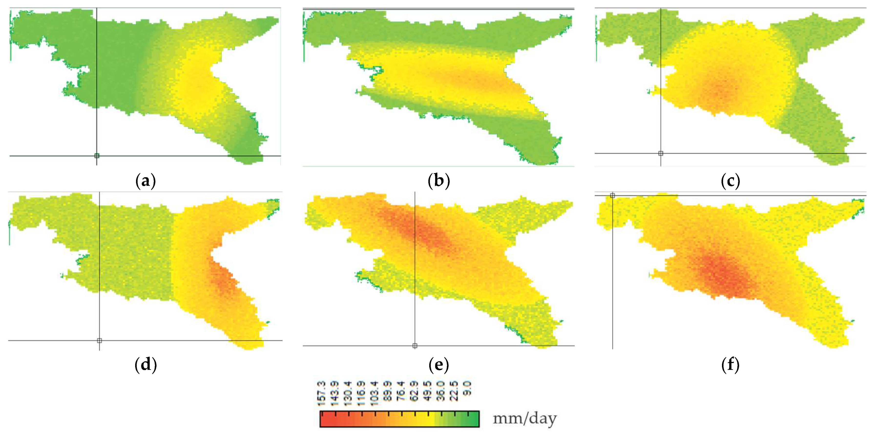
The daily rainfall data, both observed and projected, and the boundary map of the Humber River watershed were inputted into IT-NHRain, which generated the DADF curves that were used to generate the stochastic scenarios. In total, 2340 stochastic rainfall scenarios were generated (each taking about 5 min). Figure 10 shows some representative stochastic rainfall scenarios, illustrated in the CAPRA-GIS interface, that are distributed throughout the Humber River watershed. For illustrative purposes, scenarios with different locations of storm centers and for different return periods have been selected, one for each return period for the climatic scenario RCP 2.6 and the short-term period. The units are in millimeters per day, where the highest values are represented in red and the lowest in green.
3.2. Stochastic Flood Risk Assessment
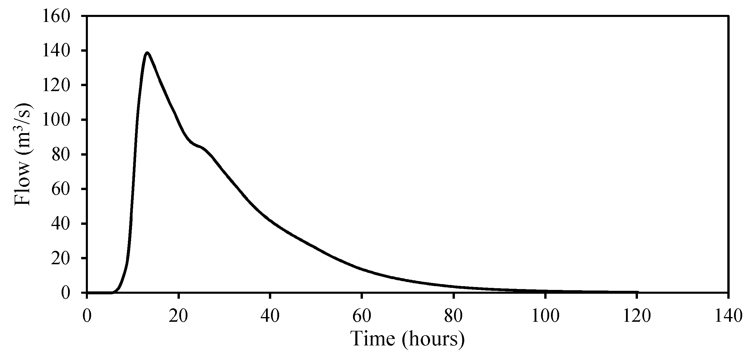
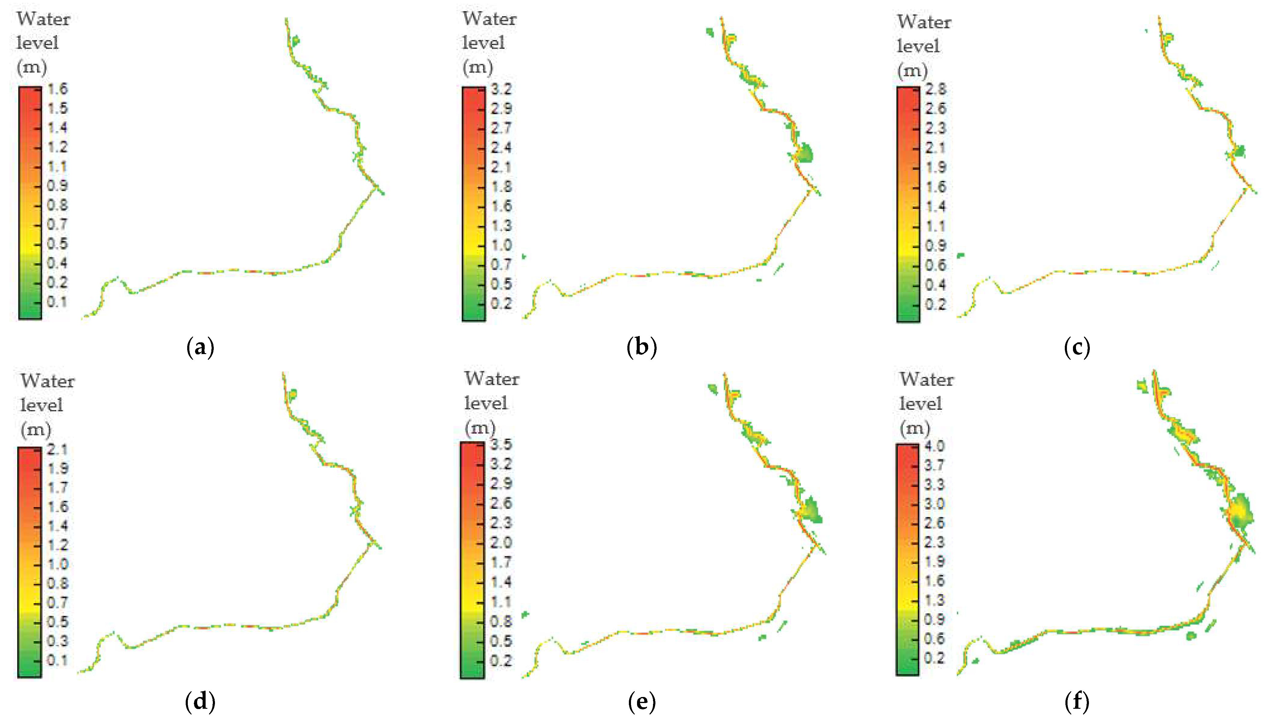
The hydrological modeling was performed for the entire Humber River watershed and considered the stochastic rainfall scenarios generated to create hydrographs for each scenario. Only the hydrographs for the Black Creek watershed were selected as input for the hydraulic modeling since the study area (Rockcliffe) is located in this watershed. For each stochastic rainfall scenario, a hydrograph was obtained. An example of one of the hydrographs generated is shown in Figure 11. Then, each hydrograph was routed through the hydraulic model to obtain the flooded areas and water depths for each stochastic rainfall scenario. This output data was then used in IT-Flood to generate the corresponding floodplain maps. Figure 12 shows a visualization of the flood scenarios in the CAPRA-GIS program, showing the flooded areas and their respective water depths in meters.
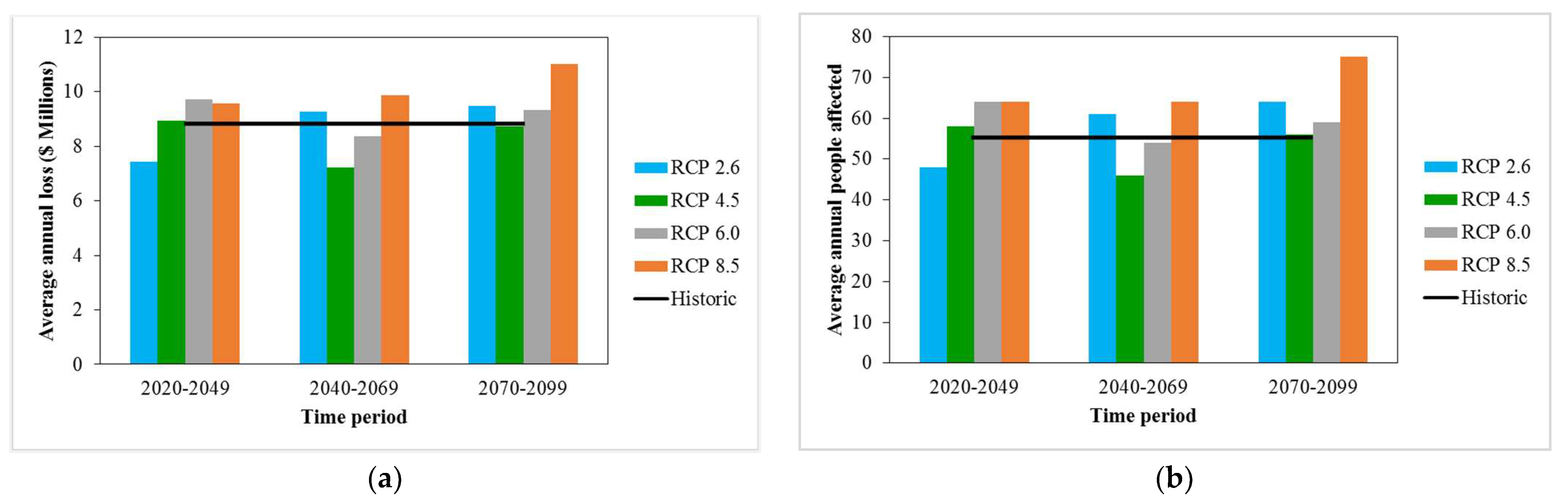
The stochastic flood scenarios were then combined with the exposure and the vulnerability functions in CAPRA-GIS to estimate the economic and social impacts associated with the historical and future rainfalls. The average annual economic and social impacts are shown in Figure 13. The figure compares the expected damages of the historic period and the three future climate change projects. The figure shows similar trends for both factors—the average annual economic losses and the number of people affected are highest for the RCP 8.5 scenario for the long-term period, followed by the RCP 2.6 period (the most optimistic scenario). For this long-term period, both factors are higher than the estimates based on the historical data for each RCP scenario except for RCP 4.5, which shows a lower amount than the historical data. Following the results of the annual rainfall analysis, the medium-term effects are lower for both factors for RCPs 4.5 and 6.0. These results show that in the near term, RCPs 6.0 and 8.5 will lead to higher economic damages and social impacts, whereas RCP 2.6 has lower impacts, which are roughly similar to the RCP 4.5 scenario. For the medium-term results, the RCP 2.6 and 8.5 scenarios resulted in higher impacts, whereas the other two scenarios resulted in lower impacts. Lastly, for the long-term simulations, all, except for the RCP 4.5 scenario, lead to higher impacts than the historic simulations. These differences in flood risk estimates are important to highlight that not all future conditions (RCPs, timelines) result in an increase in flood risk. The changes in the rainfall pattern are complex for these scenarios and result in differences between the estimates. It is important to note that future changes to land use and population within this region (which were not modeled in this study) will further affect future estimates.
These results were verified by comparing the historical results from the present analysis to those obtained by the TRCA (as part of their Flood Risk Assessment and Ranking project [35]). The average annual losses obtained in this study and in the TRCA study are $8.8 million and $8.9 million respectively, whereas the annual average of people affected found in this study and from the TRCA study are 56 and 60 people, respectively. This shows a good match between the proposed stochastic approach and the deterministic approach used in the original study. Since the TRCA analysis took into account damages to the contents of the exposed building, a higher economic loss is expected.
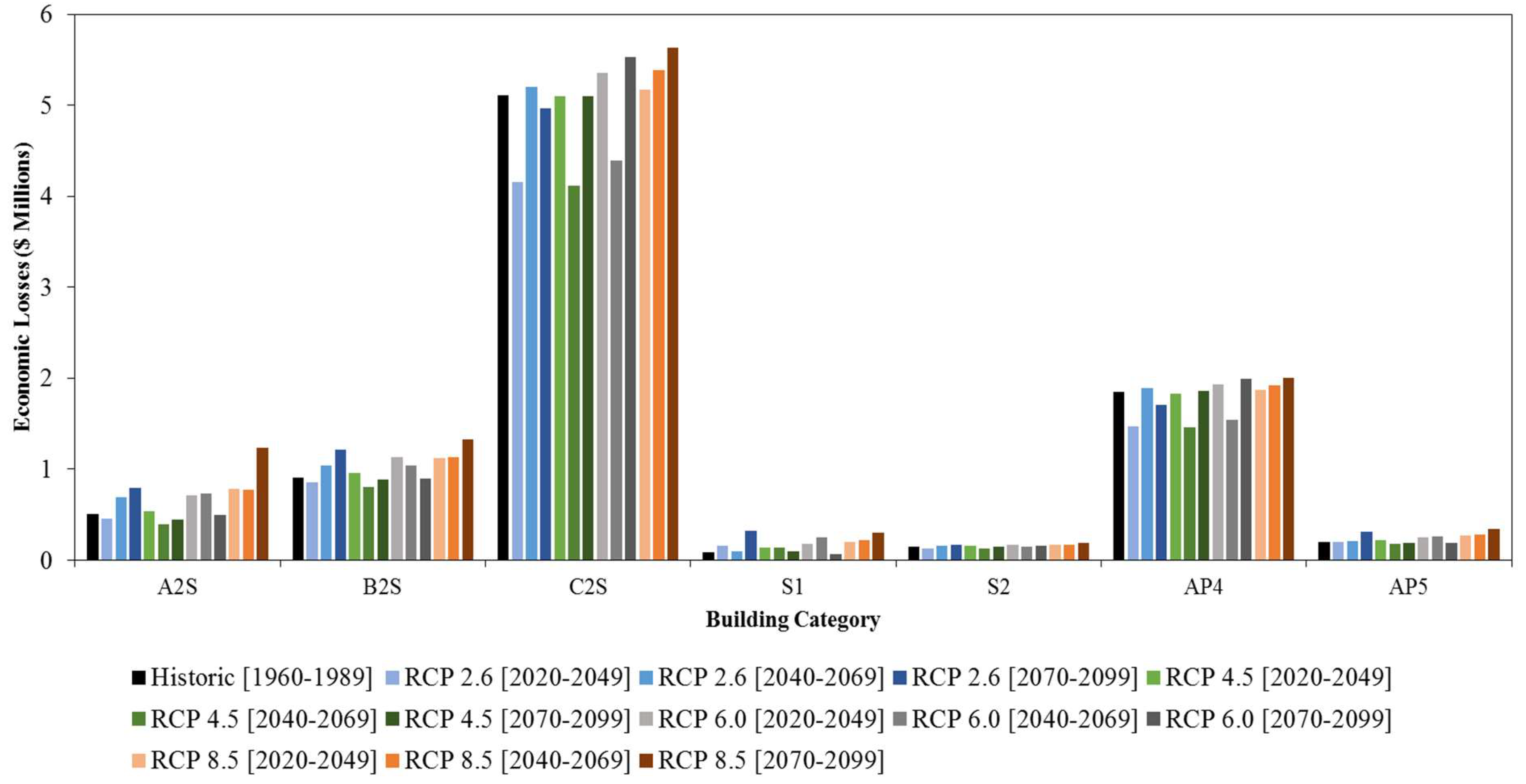
Figure 14 shows the average annual losses per building category. The category “house class C—two floors” (C2S) has by far the highest average annual losses among all the building categories for all the scenarios (between $4.1 to $5.6 million), while “office buildings” (S1), “industrial” (S2), and residential apartments with more than five floors (AP5) have the lowest (around $40.2 million). The reason why the building category C2S presents the highest average annual loss is its high vulnerability to floods (second highest) and its location with respect to the flood scenarios.
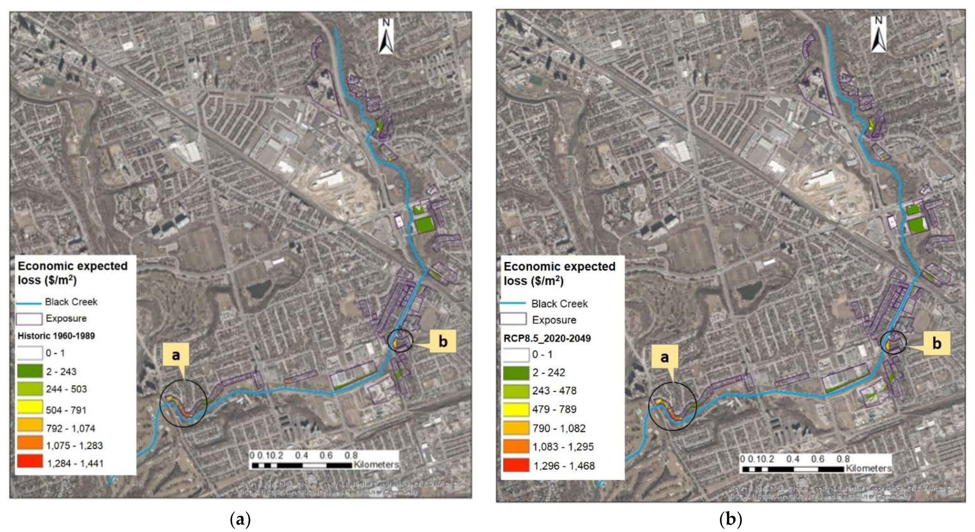
The spatial distribution of the average annual losses for all the climate scenarios allowed identifying two main clusters in the study area with the highest values. Figure 15 shows the economic expected loss maps for the historical period and the climatic scenario RCP 8.5 with the clusters identified with black circles. The cluster with the highest average annual losses (“a”) is located downstream of the Black Creek to the Westside, specifically at Black Creek Blvd close to Scarlett Rd. This area belongs to the building category “house class C—two floors” (C2S). The other cluster (“b”) is located at Humber Blvd at Hilldale Rd with the building category “apartment up to four floors” (AP4).
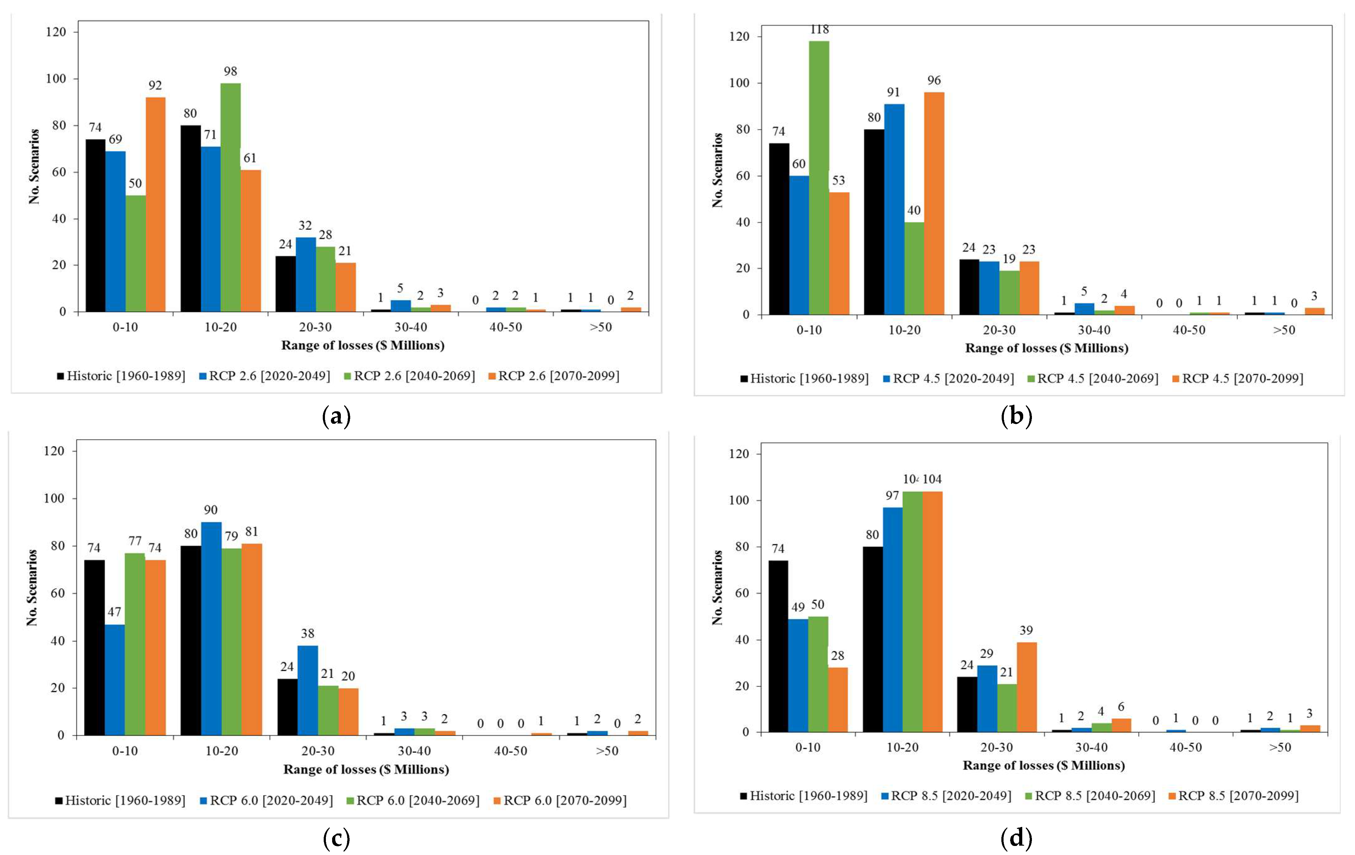
Histograms of economic expected losses were developed, which show the number of scenarios for each range of expected loss (six ranges with a bin size of $10 million). These histograms (Figure 16) show that all climate scenarios (RCPs) and time periods (short-, medium-, and long-term) have expected economic losses between $0 to $30 million, whereas only a few scenarios have economic expected losses higher than $30 million.
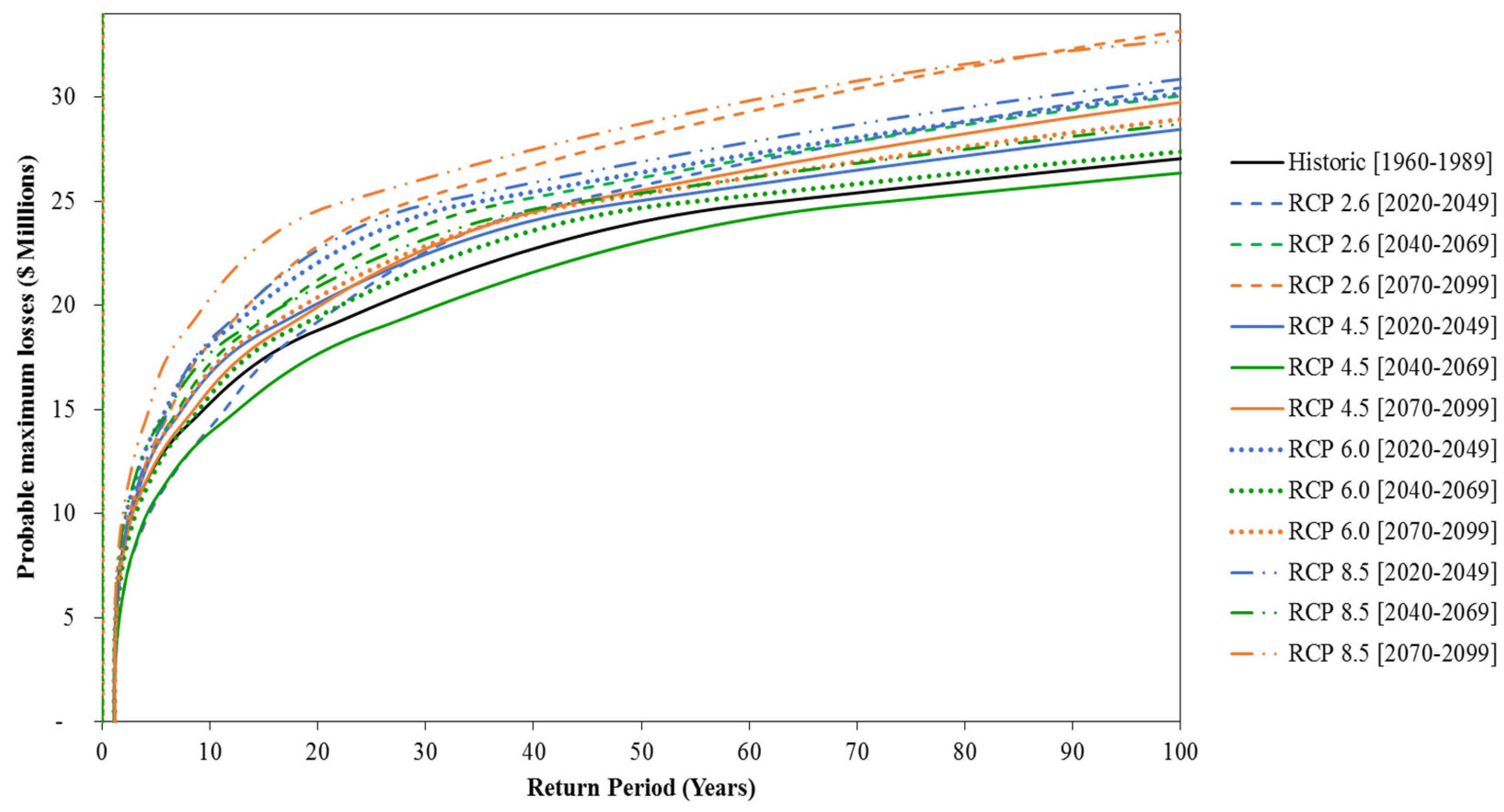
The probable maximum loss curves for all climate scenarios are shown in Figure 17. Overall, the climatic scenario RCP 8.5 for the long-term period has the highest probable maximum losses for all the return periods, except for the 100-year period for which RCP 2.6 has a higher value ($32.4 and $33.1 million, respectively). The lowest probable maximum losses correspond to the climatic scenario RCP 4.5 for the medium-term period ($25.8 million for the 100-year period), which in turn is the only one that has lower values than the historical period for all the return periods.
It is important to note that based on the results above, not all RCP scenarios lead to a higher flood hazard and risk. According to the IPCC [59], vulnerability and exposure are major drivers of risk. They vary temporally and spatially and depend on several factors, such as social, economic, geographic, and cultural, amongst others. In some cases, these factors can have a higher effect on risk than climate events. Hence, adaptation and risk reduction are more successful when considering not only the projections of the future climate but also the change in vulnerability and exposure. These factors, vulnerability and exposure, were kept constant for future periods in this study and, thus, may have a higher role to play in overall risk than the results shown here.
Unlike a deterministic approach, the stochastic framework of the risk analysis allows for obtaining results for a wide range of possible scenarios and their likelihood. It allows the risk to be expressed in terms of potential or expected losses and its comparison for different hazard conditions. In this study, the use of spatially varying rainfall scenarios was useful to analyze the impacts of the different possible hazard conditions. This gives a better understanding of the impacts of climate change on rainfall regimes and, thus, on flood hazards, and the economic and social consequences. Additionally, the risk can be expressed in terms of probable maximum losses, which is essential for establishing financial protection mechanisms [60].
In conclusion, the analysis of the stochastic rainfall shows that, in general, the future rainfall intensities will be higher, with RCP 8.5 being the most pessimistic since it resulted in the highest projected rainfall. Even though RCP 4.5 is not the most optimistic scenario, it projects the lowest rainfall. Average annual rainfalls were predicted to be higher for the long-term period and lower for the medium-term period for RCP 4.5 and RCP 6.0. It is important to highlight that the hydrological processes are a highly complex and nonlinear system, and thus, an increase in a certain amount of GHGs may not necessarily lead to an increase in rainfall throughout the different time periods.
The results show that future rainfall will lead to higher economic and social impacts due to floods. The RCP 8.5 long-term period showed the highest impacts and the RCP 4.5 medium-term period the lowest. The results also indicate higher average annual losses for the building category C2S. The area, with the highest expected economic losses, is within a neighborhood with building category C2S, located at the south of the Black Creek, in Black Creek Blvd close to Scarlett Rd. The second-highest expected economic losses were also found in a residential area, with building category AP4, located at Humber Blvd at Hilldale Rd.
3.3. Deterministic Flood Risk Assessment
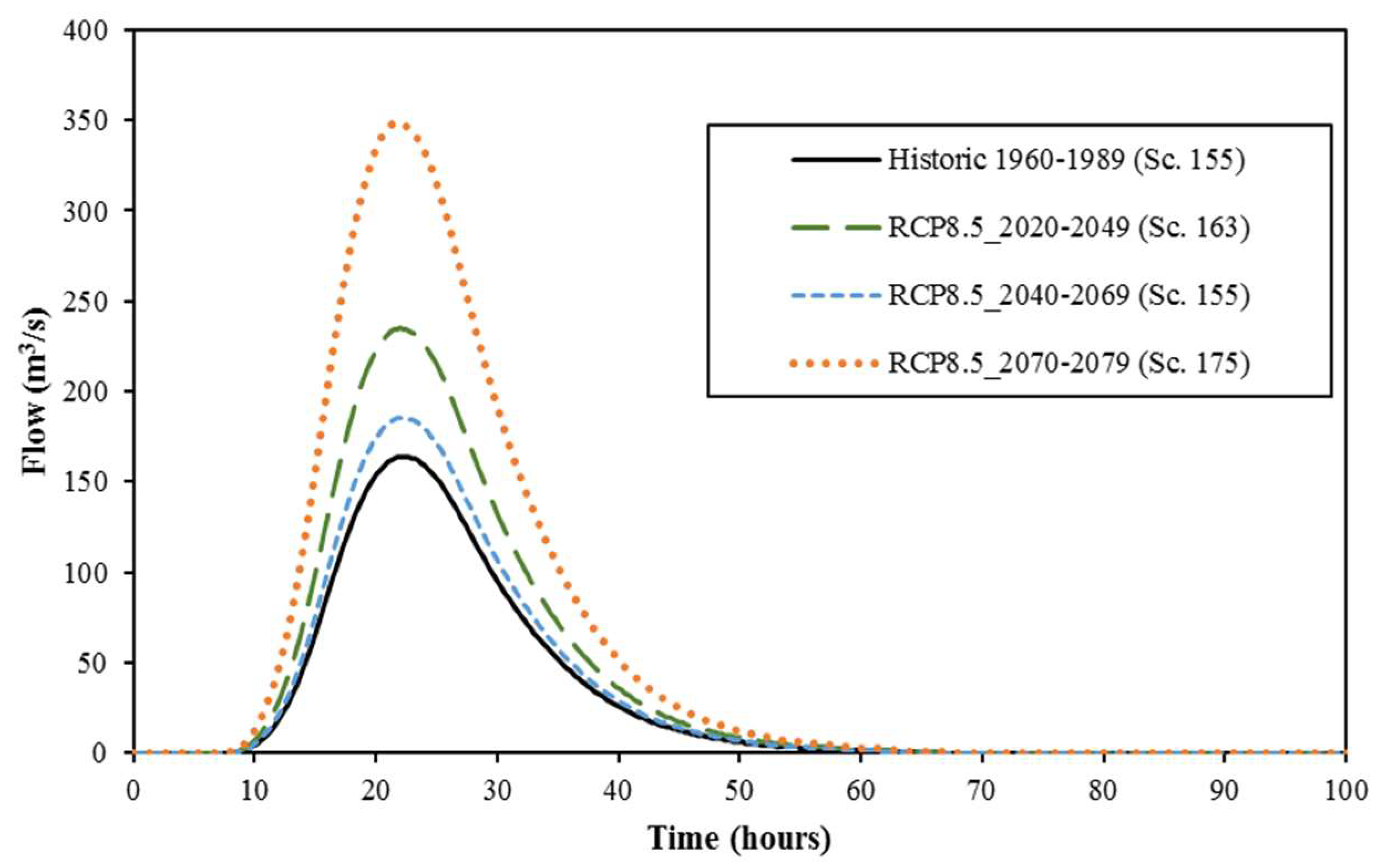
The CAPRA method allows for both stochastic and deterministic risk assessments. The stochastic analysis, presented in Section 3.2, considered the impact of all the stochastic scenarios generated and their respective likelihoods. Conversely, a deterministic analysis evaluates the impact of a single hazard scenario. In this study, the deterministic risk assessment was performed for the worst-case scenarios. This can be useful for implementing mitigation measures that not only evaluate the most probable scenarios (determined through the stochastic analysis) but also the most severe in terms of the associated impacts. The single scenarios selected to perform the deterministic flood risk assessment were obtained from the scenarios of the historic period and RCP 8.5 for each term period. Each climate scenario for a specific time period has 180 stochastic scenarios. The worst-case scenarios were identified as those with the highest expected losses out of the 180 scenarios available. Hence, the deterministic analysis was performed for the worst-case scenarios where some parameters, such as the peak flow of the runoff hydrograph (see Figure 18), the expected loss, the area affected, and the number of people affected, were obtained for each one of the four worst-case scenarios (listed in Table 4).
From this analysis, it was found that for RCP 8.5, the long-term period has the highest peak flow and the medium-term the lowest. As the peak flow is a major contribution to flooding, RCP 8.5 for the long-term period also presents the highest values in the other parameters analyzed, and the medium-term period the lowest. Amongst the four worst-case scenarios, the scenario from the historic period has the lowest values in all the parameters.
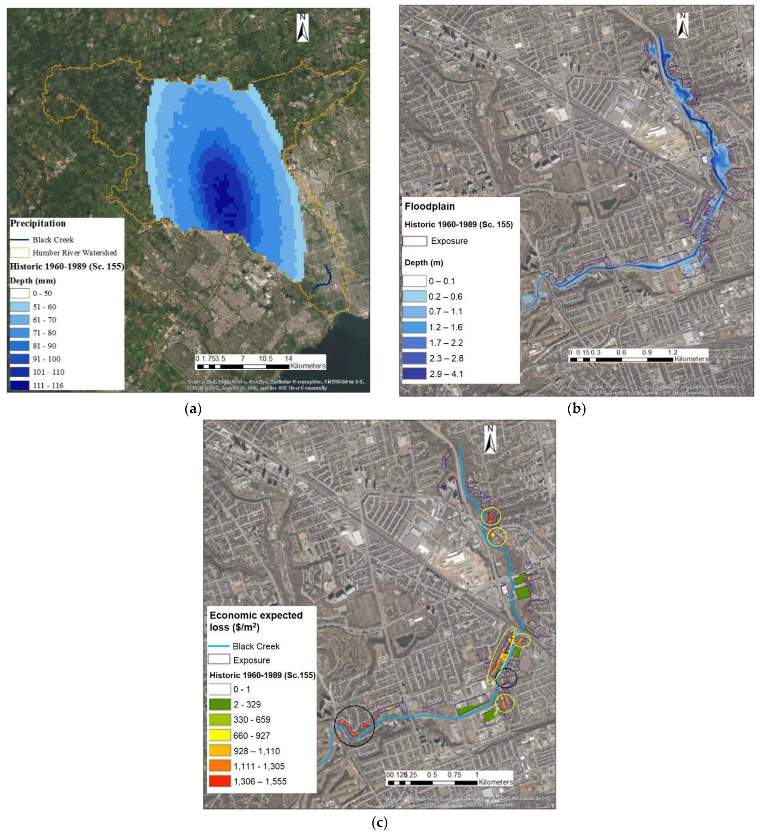
It is worth mentioning that both stochastic and deterministic risk analyses are important to highlight regions at high risk that need flood protection measures. While the stochastic results give the whole range of economic and social impacts for the different scenarios, the deterministic analysis of the selected single scenarios identifies the spatial distribution of the rainfall, the flood hazard, and its associated impacts through maps for the worst case. Figure 19 shows the rainfall map, the floodplain map, and the economic expected loss map for the historic worst-case scenario. Additionally, from the economic expected loss maps for all four worst-case scenarios, five additional clusters of high economic risk (yellow circles in Figure 19c) besides the two clusters from the stochastic assessment (black circles in Figure 19c) were found.
4. Conclusions
Several flood risk methodologies have been developed and presented in the research literature; however, many of these methods used a deterministic approach (which does not quantify the uncertainty of the risk estimates), and did not consider the effects of future climate change. Lastly, the majority of methods presented in the research only focused on economic damages rather than both economic and social damages of flood hazards.
This study aimed at performing a flood risk analysis in the Black Creek subwatershed in the Rockcliffe region in Toronto, Canada by implementing the CAPRA method, a platform for stochastic risk assessment. This framework allowed for considering the frequencies of the extreme events and to generate stochastic rainfall scenarios with random shapes, locations, and rainfall intensities based on the observed data (and hence, quantifying the uncertainty of the risk estimates). This method provided a valuable tool not only for identifying areas susceptible to floods but also to quantify the economic and social impacts and the associated probabilities of occurrence.
To quantify the flood risk of this region, we developed and applied five methods. First, we determined the stochastic rainfall hazard for the region with random shapes, locations, and rainfall intensities to quantify the uncertainty of both historical observations and projected data (for three future periods, four RCP scenarios, and six return periods). These scenarios were used to create DADF curves and spatial rainfall maps. Next, these rainfall scenarios were fed into a hydrological and hydraulic model to generate stochastic flood hazards within the region. Both the hydrological and hydraulic models were created for this region based on previous modeling efforts. The models were run in unsteady-state conditions—an improvement on previous modeling efforts. These contributions, therefore, considered both the spatial and temporal aspects of rainfall scenarios on the flood hazard. Third, we quantified the exposure of elements within the flooded area, which considered the type and value of the structures within the region. Next, we quantified the vulnerability and exposure of the exposed elements where the economic damages (via depth–damage curves) and social impacts (e.g., people exposed to floods) were quantified. Lastly, we integrated these components to determine the overall flood risk of the region and generated floodplain maps.
A major contribution of this study is that the CAPRA method can successfully recreate the historic flood risk in the region (by comparing the results to existing, deterministic risk reported for the Rockcliffe region). This allows for a better understanding of the impacts of climate change on rainfall regimes and, thus, on flood hazards and the economic and social consequences. Next, future rainfall patterns due to climate change will lead to higher economic and social impacts due to floods. The RCP 8.5 long-term period shows the highest impacts and the RCP 4.5 medium-term period the lowest. These conclusions were expected, as both scenarios had the highest and lowest rainfalls, respectively, in the rainfall hazard analysis. The reduction in flood risk due to the RCO 4.5 medium-term simulations shows that not all climate change scenarios will lead to higher flood risk. This result is important since it demonstrates the importance of other factors, such as social and economic exposure, which can have a higher contribution to risk than the flood hazard itself. The deterministic worst-case scenario from the historical period and the RCP 8.5 scenario (one for each time period) were compared based on the expected losses and the number of people affected. The lowest losses were seen for the RCP 4.5 medium-term scenario, followed by the historical period, the short-term, and the long-term RCP 8.5 scenarios.
The stochastic framework of the risk analysis provided results for a wide range of possible scenarios and their likelihood. The deterministic risk performed for the worst-case scenarios can be useful for implementing mitigation measures that not only evaluate the most probable scenarios but also the most severe in terms of the associated impacts. However, higher resolution spatio-temporal field data are needed to reveal any scaling differences in calibration of the hydraulic and hydrological models. The uncertainty of the parameters entailed in the numerical models points out the possible differences (under or overestimation) of the results obtained via the stochastic and deterministic approaches.
Recommendations for Future Research
Based on the findings of this study, the following recommendations were identified as opportunities for improving future work on flood risk assessment.
- The DEM used in this study has a resolution of 5 m. However, for creating the cross-sections for the hydraulic model, it is recommended to use a DEM with a resolution around 1 m or lower (from LiDAR or HR satellite pictures). An alternative approach may be to obtain the bathymetry of the river from a field survey.
- The current version of IT-Flood only allows for integrating the HEC-RAS 1D model. However, 2D modeling is more appropriate in several situations, for example, when the length-to-width ratio of the river is less than 3:1.
- Currently IT-NHRain only allows for generating stochastic rainfall scenarios on a daily basis. However, it may be more appropriate to use sub-daily or sub-hourly rainfall data and analyze its effect on the peak flow of hydrographs since significantly higher rainfall intensity is more likely to occur in these shorter time intervals. A recommendation to CAPRA would be to develop a version of IT-NHRain that allows for generating rainfall scenarios on a sub-daily basis.
- In this study, only seven rain gauges with rainfall data (with at least 30 years of records) were identified within the Humber River watershed. However, for such an extensive area (911 km2), the number of rain gauges may not be suitable enough to capture the spatial variation of rainfall. Moreover, several of the gauges only have daily data. An increase in the spatial density of rain gauges with a finer temporal resolution would improve the analysis (e.g., provide estimates of marginal flood risk) and ultimately may affect the outcome of the risk analysis.
- The tangible damages quantified in this study only considered direct damages. Direct damages generally consider the damage to structures and contents. A potential improvement to the quantification of damages would be to include content damages as well as indirect tangible damages (e.g., business disruption, detours, and loss of revenue).
- The social vulnerability in this study was determined only as the number of people affected based on the water depth at their place of residence. An opportunity to enhance social risk analysis would be to consider the different indicators of social vulnerability, such as demographic characteristics, socioeconomic status, land tenure, and neighborhood characteristics.
- Collaboration with the TRCA is advised to identify other possible errors in measuring key parameters, such as precipitation and discharge, that will affect the validation of the modeling results. Additional field data is required to better cover the watershed spatially and temporally in order to evaluate the results obtained via the stochastic and deterministic approaches.
Author Contributions
Conceptualization, D.R. and U.T.K.; methodology, D.R. and U.T.K.; software, D.R. and J.F.V.; formal analysis, D.R.; investigation, D.R.; data curation, D.R.; writing—original draft preparation, D.R.; writing—review and editing, J.F.V., I.T. and U.T.K.; visualization, D.R.; supervision, I.T. and U.T.K.; funding acquisition, I.T. and U.T.K. All authors have read and agreed to the published version of the manuscript.
Funding
This study was funded by the Natural Sciences and Engineering Research Council of Canada, grant numbers RGPIN-2017-05661 and RGPIN-2019-06365.
Institutional Review Board Statement
Not applicable.
Informed Consent Statement
Not applicable.
Data Availability Statement
Data available in a publicly accessible repository: The data presented in this study are openly available from Environment Canada at https://climate.weather.gc.ca/historical_data/search_historic_data_e.html, accessed on 10 February 2019 and the Ontario Climate Data Portal at: https://lamps.math.yorku.ca/OntarioClimate/, accessed on 10 February 2019. 3rd Party Data: Restrictions apply to the availability of the data (hydrological and hydraulic models). These models were obtained from the Toronto and Region Conservation Authority and are available directly from them.
Acknowledgments
The authors would like to thank the Toronto and Region Conservation Authority for providing the hydrological and hydraulic model used as the basis of this study, and other data used for the risk analyses component. We also acknowledge the Lassonde School of Engineering at York University for providing graduate student support for D.R.
Conflicts of Interest
The authors declare no conflict of interest.
References
- Abdallah, C.; Hdeib, R. Flood risk assessment and mapping for the Lebanese watersheds. In Proceedings of the EGU General Assembly Conference, Vienna, Austria, 17–22 April 2016. [Google Scholar]
- Lopardo, R.A.; Seoane, R. Algunas reflexiones sobre crecidas e inundaciones. Ing. Agua 2000, 7, 11–21. [Google Scholar] [CrossRef] [Green Version]
- Cruickshank, V.C. Modelos Para el Tránsito de Avenidas en Cauces Con Llanuras de Inundación. Plan Nacional Hidráulico. Gobierno de la Federación. México. 1974. Available online: https://www.slideshare.net/AcademiaDeIngenieriaMx/plan-nacional-hidrulico (accessed on 8 January 2022).
- Zwenzner, H.; Voigt, S. Improved estimation of flood parameters by combining space based SAR data with very high resolution digital elevation data. Hydrol. Earth Syst. Sci. 2009, 13, 567–576. [Google Scholar] [CrossRef] [Green Version]
- Keating, A.; Campbell, K.; Mechler, R.; Michel-Kerjan, E.; Mochizuki, J.; Kunreuther, H.; Bayer, J.; Hanger, S.; McCallum, I.; See, L.; et al. Operationalizing Resilience against Natural Disaster Risk: Opportunities, Barriers and a Way forward. Laxenburg, Austria: Zurich Flood Resilience Alliance, International Institute for Applied Systems Analysis. 2014. Available online: http://pure.iiasa.ac.at/id/eprint/11191 (accessed on 8 January 2022).
- Arnell, N.W.; Gosling, S.N. The impacts of climate change on river flood risk at the global scale. Clim. Change 2016, 134, 387–401. [Google Scholar] [CrossRef] [Green Version]
- Ontario Climate Date Portal (OCDP). Trends of Rainfall in Ontario. LAMPS, Department of Mathematics and Statistics, York University. 2018. Available online: http://lamps.math.yorku.ca/OntarioClimate (accessed on 10 February 2019).
- Thieken, A.H.; Olschewski, A.; Kreibich, H.; Kobsch, S.; Merz, B. Development and evaluation of FLEMOps—A new Flood Loss Estimation MOdel for the private sector. WIT Trans. Ecol. Environ. 2008, 118, 315–324. [Google Scholar] [CrossRef]
- Meyer, V.; Scheuer, S.; Haase, D. A multicriteria approach for flood risk mapping exemplified at the Mulde river, Germany. Nat. Hazards 2009, 48, 17–39. [Google Scholar] [CrossRef]
- Kubal, C.; Haase, D.; Meyer, V.; Scheuer, S. Integrated urban flood risk assessment—Adapting a multicriteria approach to a city. Nat. Hazards Earth Syst. Sci. 2009, 9, 1881–1895. [Google Scholar] [CrossRef] [Green Version]
- Dottori, F.; Figueiredo, R.; Martina, M.L.; Molinari, D.; Scorzini, A.R. INSYDE: A synthetic, probabilistic flood damage model based on explicit cost analysis. Nat. Hazards Earth Syst. Sci. 2016, 16, 2577–2591. [Google Scholar] [CrossRef] [Green Version]
- Escuder-Bueno, I.; Castillo-Rodrıguez, J.T.; Perales-Momparler, S.; Morales-Torres, A. SUFRI Method for Pluvial and River Flooding Risk Assessment in Urban Areas to Inform Decision Making. In WP3 Final Report, SUFRI Project (Sustainable Strategies of Urban Flood Risk Management), Valencia, Comunitat Valenciana. Spain: Polytechnic University of Valencia. Research Institute of Water and Environmental Engineering. 2011. Available online: http://www.edams.upv.es/docs/2011_July_SUFRI_WP3_Final%20Report.pdf (accessed on 27 May 2018).
- King, A.; Bell, R. Riskscape New Zealand—A Multihazard Loss Modelling Tool. In Proceedings of the NZSEE Conference, Napier, New Zealand, 10–12 March 2006; pp. 30.1–30.9. [Google Scholar]
- Deckers, P.; Kellens, W.; Reyns, J.; Vanneuville, E.; Maeyer, P. A GIS for Flood Risk Management in Flanders. In Geospatial Techniques in Urban Hazard and Disaster Analysis; Showalter, P.S., Yongmei, L., Eds.; Springer: Dodrecht, The Netherlands, 2009; pp. 51–69. [Google Scholar]
- USACE. Flood Impact Analysis_HEC-FIA User’s Manual, Version 3.0; U.S. Army Corps of Engineers: Davis, CA, USA; Washington, DC, USA, 2015.
- Scawthorn, C.; Flores, P.; Blais, N.; Seligson, H.; Tate, E.; Chang, S.; Mifflin, E.; Thomas, W.; Murphy, J.; Jones, C.; et al. HAZUS-MH flood loss estimation methodology. II. Damage and loss assessment. Nat. Hazards Rev. 2006, 7, 72–81. [Google Scholar] [CrossRef]
- Cardona, O.D.; Ordaz, M.; Reinoso, E.; Yamín, L.E.; Barbat, A. CAPRA-comprehensive approach to probabilistic risk assessment: International initiative for risk management effectiveness. In Proceedings of the 15th World Conference of Earthquake Engineering, Lisbon, Portugal, 24–28 September 2012; Volume 1, pp. 4259–4268. [Google Scholar]
- Nicholas, J.; Holt, G.D.; Proverbs, D.G. Towards standardizing the assessment of flood damaged properties in the UK. Struct. Survey 2001, 19, 163–172. [Google Scholar] [CrossRef]
- Zhai, G.; Fukuzono, T.; Ikeda, S. Modeling flood damage: Case of Tokai Flood 2000. J. Am. Water Res. Assoc. 2005, 41, 77–92. [Google Scholar] [CrossRef]
- Su, M.D.; Kang, J.L.; Chang, L.F.; Chen, A.S. A grid-based GIS approach to regional flood damage assessment. J. Mar. Sci. Technol. 2005, 13, 184–192. [Google Scholar] [CrossRef]
- Ernst, J.; Dewals, B.; Archambeau, P.; Detrembleur, S.; Erpicum, S.; Pirotton, M. Integration of accurate 2D inundation modelling, vector land use database and economic damage evaluation. In Proceedings of the European Conference on Flood Risk Management—Floodrisk, Oxford, UK, 30 September–2 October 2008; Taylor & Francis: London, UK, 2008; pp. 1643–1653. [Google Scholar]
- Schwarz, J.; Maiwald, H. Damage and loss prediction model based on the vulnerability of building types. In Proceedings of the 4th International Symposium on Flood Defence: Managing Flood Risk, Reliability and Vulnerability, Toronto, ON, Canada, 6–8 May 2008; GFZ: Potsdam, Germany, 2008; pp. 1–9. [Google Scholar] [CrossRef]
- Belger, G.; Haase, M.; Jung, T.; Lippert, K. A GIS-based Platform for Environmental and Water Resources Modeling—Kalypso Open Source. GEO Inform. 2009, 12, 36–39. [Google Scholar]
- USACE. Flood Damage Reduction Analysis _HEC-FDA User’s Manual, Version 1.4.1; U.S. Army Corps of Engineers: Davis, CA, USA; Washington, DC, USA, 2016.
- Vozinaki, A.E.; Karatzas, G.P.; Sibetheros, I.A.; Varouchakis, E.A. An agricultural flash flood loss estimation methodology: The case study of the Koiliaris basin (Greece), February 2003 flood. Nat. Hazards 2015, 79, 899–920. [Google Scholar] [CrossRef]
- Dutta, D.; Herath, S.; Musiake, K. A mathematical model for flood loss estimation. J. Hydrol. 2003, 277, 24–49. [Google Scholar] [CrossRef]
- Tsakiris, G.; Pistrika, A.; Klampanos, I.; Laoupi, A.; Ioannidis, C.; Soile, S.; Georgopoulos, A. DISMA—Disaster Management GIS with emphasis on cultural sites—Technical Report—Volume I (unpublished); INTERREG IIIC—Sud Initiative and the Regional Operation Framework of NOE Programme; Centre for the Assessment of Natural Hazards and Proactive Planning, National Technical University of Athens: Athens, Greece, 2007. [Google Scholar]
- Evaluación de Riesgos Naturales-América Latina (ERN-AL). Central America Probabilistic Risk Assessment—CAPRA; World Bank and Inter-American Development Bank (IDB): Washington, DC, USA, 2008; Available online: https://ecapra.org/ (accessed on 12 January 2022).
- Kappes, M.S.; Keiler, M.; von Elverfeldt, K.; Glade, T. Challenges of analyzing multi-hazard risk: A review. Nat. Hazards 2012, 64, 1925–1958. [Google Scholar] [CrossRef] [Green Version]
- Marulanda, M.C.; Carreño, M.L.; Cardona, O.D.; Ordaz, M.; Barbat, A.H. Probabilistic Earthquake Risk Assessment Using CAPRA: Application to the City of Barcelona, Spain. Nat. Hazards 2013, 69, 59–84. [Google Scholar] [CrossRef]
- Torres, M.A.; Jaimes, M.A.; Reinoso, E.; Ordaz, M. Event-Based Approach for Probabilistic Flood Risk Assessment. Int. J. River Basin Manag. 2013, 12, 377–389. [Google Scholar] [CrossRef]
- IDB. Estimación de la Amenaza y el Riesgo Probabilista por Huracán en Guatemala, Incorporando el Impacto Asociado al Cambio Climático. (Technical Note IDB-TN-667); IDB: Madrid, Spain, 2014. (In Spanish) [Google Scholar]
- Cardona, O.D.; Bernal, G.A.; Ordaz, M.G.; Salgado-Gálvez, M.A.; Singh, S.K.; Mora, M.G.; Villegas, C.P. Update on the Probabilistic Modelling of Natural Risks at Global Level: Global Risk Model—Global Earthquake and Tropical Cyclone Hazard Assessment. Disaster Risk Assessment at Country Level for Earthquakes, Tropical Cyclones (Wind and Storm Surge), Floods, Tsunami and Volcanic Eruptions. Background Paper for GAR15. Barcelona/Bogotá; United Nations International Strategy for Disaster Risk Reduction (UNISDR): Geneva, Switzerland, 2015. [Google Scholar]
- Reinoso, E.; Ordaz, M.; Cardona, O.D.; Bernal, G.A.; Contreras-Zazuera, M. After 10 Years of CAPRA. Conference: 16th European Conference on Earthquake Engineering 16ECEEAt: Thessaloniki. 2018. Available online: http://papers.16ecee.org/files/Contribution%2012062.pdf (accessed on 3 May 2020).
- Toronto Region Conservation Authority (TRCA). Flood Risk Assessment and Ranking of Flood Vulnerable Clusters. 2019. Available online: https://conservationontario.ca/fileadmin/pdf/conservation_authorities_tech_transfer/TechTransfer2019_10_Plato_Flood_Risk_Assessment_and_Ranking.pdf (accessed on 18 March 2019).
- Bonell, J.L. Remembering the Don. In Reclaiming the Don: An Environmental History of Toronto’s Don River Valle; University of Toronto Press: Toronto, ON, Canada, 2014; pp. 173–188. [Google Scholar]
- Wateroffice. Daily Discharge Data for BLACK CREEK NEAR WESTON (02HC027). 2021. Available online: https://wateroffice.ec.gc.ca/report/historical_e.html?start_year=1850&end_year=2021&mean1=1&scale=normal&mode=Table&stn=02HC027&dataType=Daily¶meterType=Flow&year=2020&page=historical (accessed on 26 December 2021).
- Toronto Region Conservation Authority. Black Creek (Rockcliffe Area) Riverine Flood Management. Class Environmental Assessment; AMEC: Burlington, ON, Canada, 2014. [Google Scholar]
- IPCC. Climate Change 2013: The Physical Science Basis. Contribution of Working Group I to the Fifth Assessment Report of the Intergovernmental Panel on Climate Change; Cambridge University Press: Cambridge, UK, 2013. [Google Scholar] [CrossRef] [Green Version]
- Moss, R.H.; Edmonds, J.A.; Hibbard, K.A.; Manning, M.R.; Rose, S.K.; van Vuuren, D.P.; Carter, T.R.; Emori, S.; Kainuma, M.; Kram, T.; et al. The next generation of scenarios for climate change research and assessment. Nature 2010, 463, 747–756. [Google Scholar] [CrossRef]
- Ruiter, A. Delta-Change Approach for CMIP5 GMCs, Trainee Report at Royal Netherlands Meteorological Institute. 2012. Available online: http://bibliotheek.knmi.nl/stageverslagen (accessed on 22 February 2019).
- Evaluación de Riesgos Naturales-América Latina (ERN-AL). IT-NHRain User’s Manual. 2009. Available online: https://ecapra.org/topics/ern-nhrain (accessed on 21 May 2018).
- Hogg, W.D. Time distribution of short duration storm rainfall in Canada. In Proceedings of the Canadian Hydrology Symposium, Toronto, ON, Canada, 26–27 May 1980; National Research Council of Canada: Ottawa, ON, Canada, 1982; pp. 53–63. [Google Scholar]
- CIVICA. Final Report: Humber River Hydrology Update. 2018. Available online: https://trca.ca/app/uploads/2016/07/Humber-Hydrology-Update-Final-Report-v19.1.pdf (accessed on 15 June 2018).
- Vojtek, M.; Petroselli, A.; Vojteková, J.; Asgharinia, S. Flood inundation mapping in small and ungauged basins: Sensitivity analysis using the EBA4SUB and HEC-RAS modeling approach. Hydrol. Res. 2019, 50, 1002–1019. [Google Scholar] [CrossRef] [Green Version]
- Pellicani, R.; Parisi, A.; Lemmolo, G.; Apollonio, C. Economic Risk Evaluation in Urban Flooding and Instability-Prone Areas: The Case Study of San Giovanni Rotondo (Southern Italy). Geosciences 2018, 8, 112. [Google Scholar] [CrossRef] [Green Version]
- Nicklin, H.; Leicher, A.M.; Dieperink, C.; Van Leeuwen, K. Understanding the costs of inaction–an assessment of pluvial flood damages in two European cities. Water 2019, 11, 801. [Google Scholar] [CrossRef] [Green Version]
- Van Ackere, S. Flood Impact Assessment Tool (FLIAT) An Object-Relational GIS Tool for Flood Impact Assessment in Flanders, Belgium. Ph.D. Thesis, Department of Geography, Faculty of Science, Ghent University, Ghent, Belgium, 2019. [Google Scholar]
- Habermann, N.; Hedel, R. Damage functions for transport infrastructure. Int. J. Disaster Resil. Built Environ. 2018, 9, 420–434. [Google Scholar] [CrossRef] [Green Version]
- Associated Programme on Flood Management. Risk Management for Flood. What Are the Negative Social Impacts of Flooding? Available online: https://www.floodmanagement.info/what-are-the-negative-social-impacts-of-flooding/2013 (accessed on 24 July 2018).
- Statistics Canada. Census Tracts. 2016. Available online: http://www12.statcan.gc.ca/census-recensement/2011/geo/bound-limit/bound-limit-2016-eng.cfm (accessed on 5 February 2018).
- Kron, W. Flood Risk = Hazard • Values • Vulnerability. Water Int. 2005, 30, 58–68. [Google Scholar] [CrossRef]
- Natural Resources Canada. Canadian Guidelines and Database of Flood Vulnerability Functions; Canadian Floodplain Mapping Guidelines Series; Natural Resources Canada: Ottawa, ON, Canada, 2017.
- Rufat, S.; Tate, E.; Burton, C.G.; Maroof, A.S. Social vulnerability to floods: Review of case studies and implications for measurement. Int. J. Disaster Risk Reduct. 2015, 14, 470–486. [Google Scholar] [CrossRef] [Green Version]
- Rincón, D.; Khan, U.T.; Armenakis, C. Flood risk mapping using GIS and multi-criteria analysis: A greater Toronto area case study. Geosciences 2018, 8, 275. [Google Scholar] [CrossRef] [Green Version]
- Yamin, L.E.; Hurtado, A.I.; Barbat, A.H.; Cardona, O.D. Seismic and wind vulnerability assessment for the GAR-13 global risk assessment. Int. J. Disaster Risk Reduct. 2014, 10, 452–460. [Google Scholar] [CrossRef] [Green Version]
- Peduzzi, P.; Dao, H.; Herold, C.; Mouton, F. Assessing global exposure and vulnerability towards natural hazards: The Disaster Risk Index. Nat. Hazards Earth Syst. 2009, 9, 1149–1159. [Google Scholar] [CrossRef]
- Samuels, P.; Gouldby, B. Language of Risk—Project Definitions. T32-04-01, 2nd ed.; Integrated Flood Risk Analysis and Management Methodologies, FLOODsite; 2009; Available online: http://floodsite.net/html/partner_area/project_docs (accessed on 20 January 2019).
- Cardona, D.O.; van Aalst, M.K.; Birkmann, J.; Fordham, M.; McGregor, G.; Perez, R.; Pulwarty, R.S.; Schipper, E.L.F.; Sinh, B.T. Determinants of risk: Exposure and vulnerability. In Managing the Risks of Extreme Events and Disasters to Advance Climate Change Adaptation; Field, C.B., Barros, T.F.V., Stocker, D., Qin, D.J., Dokken, K.L., Ebi, M.D., Mastrandrea, K.J., Mach, G.-K., Plattner, S.K., Allen, M., et al., Eds.; A Special Report of Working Groups I and II of the Intergovernmental Panel on Climate Change (IPCC); Cambridge University Press: Cambridge, UK; New York, NY, USA, 2012; pp. 65–108. [Google Scholar]
- León, N. Implementación de los Programas HEC-HMS y HEC-RAS en la Plataforma CAPRA Para Evaluación de Riesgo Por Inundación. Ph.D. Thesis, Departamento de Ingeniería Civil y Ambiental, Universidad de Los Andes, Bogotá, Colombia, 2014. [Google Scholar]
Figure 1.
Major flood events in Toronto in the last century.

Figure 2.
Study area: Rockcliffe region within the Black Creek subwatershed.

Figure 3.
Map of the rain gauges selected in the Humber River watershed.

Figure 4.
DADF curves for the historical period (1960 to 1989).

Figure 5.
Sequence of the steps for the generation of stochastic flood scenarios.

Figure 6.
Exposure map classification: (a) economic value; (b) building category; (c) population.

Figure 7.
Residential and non-residential depth–damage curves (%).

Figure 8.
Social depth–damage curve (%).

Figure 9.
A comparison of projected annual rainfall for each time period (for different GCMs) and the observed historical values. The dots in the figure represent outliers in the data.
Figure 9.
A comparison of projected annual rainfall for each time period (for different GCMs) and the observed historical values. The dots in the figure represent outliers in the data.

Figure 10.
Illustrative examples of stochastic rainfall scenarios for the climatic scenario RCP 2.6 and the short-term period for the return periods of (a) 2 years; (b) 5 years; (c) 10 years; (d) 25 years; (e) 50 years; (f) 100 years (mm).
Figure 10.
Illustrative examples of stochastic rainfall scenarios for the climatic scenario RCP 2.6 and the short-term period for the return periods of (a) 2 years; (b) 5 years; (c) 10 years; (d) 25 years; (e) 50 years; (f) 100 years (mm).

Figure 11.
Example of a hydrograph of one of the stochastic scenarios (RCP 4.5, 10-year return period).
Figure 11.
Example of a hydrograph of one of the stochastic scenarios (RCP 4.5, 10-year return period).

Figure 12.
Illustrative example of stochastic flood scenarios for the climatic scenario RCP 2.6 and the short-term period for the return periods of (a) 2 years; (b) 5 years; (c) 10 years; (d) 25 years; (e) 50 years; (f) 100 years.
Figure 12.
Illustrative example of stochastic flood scenarios for the climatic scenario RCP 2.6 and the short-term period for the return periods of (a) 2 years; (b) 5 years; (c) 10 years; (d) 25 years; (e) 50 years; (f) 100 years.

Figure 13.
Average annual impacts plots. (a) Economic loss; (b) affected people.

Figure 14.
Economic expected losses per building category.

Figure 15.
Economic expected loss maps for the (a) historic period and RCP 8.5 (b) short-term period; (c) medium-term period; (d) long-term period.
Figure 15.
Economic expected loss maps for the (a) historic period and RCP 8.5 (b) short-term period; (c) medium-term period; (d) long-term period.


Figure 16.
Histogram of economic expected losses for (a) RCP 2.6; (b) RCP 4.5; (c) RCP 6.0; (d) RCP 8.5.
Figure 16.
Histogram of economic expected losses for (a) RCP 2.6; (b) RCP 4.5; (c) RCP 6.0; (d) RCP 8.5.

Figure 17.
Probable maximum loss curves.

Figure 18.
Hydrographs for the worst-case scenario (where Sc refers to the scenario number).

Figure 19.
Results for the worst-case scenario of the historical period (Scenario 155). (a) Rainfall map; (b) floodplain map; (c) economic expected loss map.
Figure 19.
Results for the worst-case scenario of the historical period (Scenario 155). (a) Rainfall map; (b) floodplain map; (c) economic expected loss map.


Table 1.
Characteristics of the different methods for flood risk assessment.
| Method | Source | Location | Economic Impacts | Social Impacts | Software | Hydrological Hydraulic Model |
|---|---|---|---|---|---|---|
| Flood Loss Estimation Model (FLEMO) | [8] | Germany | Buildings (Deterministic) | No | No | No |
| FloodCalc | [9,10] | Germany | Buildings (Probabilistic, Expected Annual Damage) | Yes (Annual average affected population, probability of social hot spots) | Yes (Open source) | No |
| In-depth Synthetic Model for Flood Damage Estimation (INSYDE) | [11] | Italy | Buildings (Deterministic) | No | No | No |
| Strategies of Urban Flood Risk Management (SUFRI) | [12] | Europe | Buildings (Probabilistic Expected Annual Damage) | Yes (Potential fatalities) | No | No |
| Towards standardizing the assessment of flood-damaged properties in the UK | [18] | UK | Buildings (Deterministic) | No | No | No |
| Doughnut Structure Model | [19] | Japan | Buildings (Deterministic) | No | No | No |
| A Grid-Based GIS Approach to Regional Flood Damage Assessment | [20] | Taiwan | Buildings (Probabilistic, Expected Annual Damage) | No | No | Hydrological: HEC-1 Hydraulic: 1D dynamic channel flow routing, 2D overland-flow routing |
| Decision Support System (DSS) combined with cost-benefit and multi-criteria analysis | [21] | Belgium | Buildings (Deterministic) | No | No | Hydrological: No Hydraulic: WOLF 2D |
| Vulnerability of building types | [22] | Germany | Buildings (Deterministic) | No | No | No |
| Kalypso | [23] | Germany | Buildings (Probabilistic, Expected Annual Damage) | No | Yes (Open source) | Hydrological: Kalypso Hydrology Hydraulic: Kalypso WSPM Kalypso 1D/2D |
| Hydrologic Engineering Center—Flood Damage Reduction Analysis (HEC-FDA) | [24] | US | Buildings (Probabilistic, Expected Annual Damage, Equivalent Annual Damages, Annual Exceedance Probability) | No | Yes (Not open source) | Hydrological: HEC-HMS Hydraulic: HEC-RAS |
| RiskScape | [13] | New Zealand | Buildings (Deterministic) | Yes (Fatalities, injuries) | Yes (Open source) | No |
| Agricultural flash flood | [25] | Greece | Agriculture (Deterministic) | No | No | Hydrological: No Hydraulic: MIKE FLOOD |
| Mathematical Model for flood loss estimation | [26] | Japan | Buildings, Agriculture (Deterministic) | No | No | Hydrological: Yes Hydraulic: 1D and 2D |
| Hazus-MH Flood Model | [16] | US | Buildings, Agriculture (Probabilistic, Expected Annual Damage) | Yes (Fatalities, shelter) | Yes (Not open source) | Hydrological/ Hydraulic: HAZUZ-MH |
| LATIS | [14] | Belgium | Buildings, Agriculture (Probabilistic, Expected Annual Damage) | Yes (Fatalities) | Yes (Not open source) | No |
| GIS-based tool for flood direct damage | [27] | Greece | Buildings, Agriculture (Deterministic) | No | Yes (Not open source) | No |
| Hydrologic Engineering Center—Flood Impact Analysis (HEC-FIA) | [15] | US | Buildings, Agriculture (Deterministic) | Yes (Fatalities) | Yes (Not open source) | No |
| CAPRA | [17] | Central America | Buildings, Agriculture (Probabilistic, Expected Annual Damage, Probable Maximum Loss, Loss curve) | Yes (Fatalities) | Yes (Open source) | Hydrological: HEC-HMS Hydraulic: HEC-RAS |
Table 2.
Economic values per building category.
| Category | Subcategory | Specification | ID | Value ($/m2) |
|---|---|---|---|---|
| Non-residential | Office buildings | 5 floors or less (with surface parking) | S1 | 2314 |
| Industrial | 28′ Clear height (20,000–50,000 sq. ft.) | S2 | 1022 | |
| Residential | House Class A—two floors | High-quality construction materials and finishes | A2S | 4198 |
| House Class B—two floors | Medium-quality construction materials and finishes | B2S | ||
| House Class C—two floors | Low-quality construction materials and finishes | C2S | ||
| Apartment up to four floors | High-quality | AP4 | ||
| Apartment from five floors | High-quality | AP5 |
Table 3.
Exposed area, exposed value, and exposed people per building category.
| Building’s ID | Exposed Area | Exposed Value | Exposed People | |||
|---|---|---|---|---|---|---|
| m2 | % | ($) | % | # of People | % | |
| A2S | 41,489 | 8.7 | 174,190,106 | 11.5 | 119 | 5.2 |
| B2S | 116,039 | 24.2 | 487,133,836 | 32.2 | 584 | 25.7 |
| C2S | 63,499 | 13.2 | 266,577,763 | 17.6 | 252 | 11.1 |
| S1 | 34,655 | 7.2 | 80,222,569 | 5.3 | 131 | 5.8 |
| S2 | 136,137 | 28.4 | 139,283,066 | 9.2 | 586 | 25.7 |
| AP4 | 20,828 | 4.3 | 87,470,653 | 5.8 | 66 | 2.9 |
| AP5 | 66,702 | 13.9 | 280,006,743 | 18.5 | 539 | 23.6 |
| Total | 479,349 | 100 | 1,514,884,735 | 100 | 2277 | 100 |
Table 4.
Parameters of the worst-case scenarios.
| ID | Scenario | Time Period | Peak Flow (m3/s) | Expected Loss ($) | Area Affected (m2) | People Affected |
|---|---|---|---|---|---|---|
| 155 | Historic | 1960–1989 | 163.8 | 53,489,348 | 125,769 | 517 |
| 163 | RCP 8.5 | 2020–2049 | 234.9 | 71,568,513 | 149,243 | 617 |
| 155 | 2040–2069 | 185.4 | 50,979,159 | 122,918 | 504 | |
| 175 | 2070–2079 | 348.3 | 88,327,427 | 170,360 | 705 |
Publisher’s Note: MDPI stays neutral with regard to jurisdictional claims in published maps and institutional affiliations. |
© 2022 by the authors. Licensee MDPI, Basel, Switzerland. This article is an open access article distributed under the terms and conditions of the Creative Commons Attribution (CC BY) license (https://creativecommons.org/licenses/by/4.0/).
Share and Cite
MDPI and ACS Style
Rincón, D.; Velandia, J.F.; Tsanis, I.; Khan, U.T. Stochastic Flood Risk Assessment under Climate Change Scenarios for Toronto, Canada Using CAPRA. Water 2022, 14, 227. https://doi.org/10.3390/w14020227
AMA Style
Rincón D, Velandia JF, Tsanis I, Khan UT. Stochastic Flood Risk Assessment under Climate Change Scenarios for Toronto, Canada Using CAPRA. Water. 2022; 14(2):227. https://doi.org/10.3390/w14020227
Chicago/Turabian StyleRincón, Daniela, Juan Felipe Velandia, Ioannis Tsanis, and Usman T. Khan. 2022. "Stochastic Flood Risk Assessment under Climate Change Scenarios for Toronto, Canada Using CAPRA" Water 14, no. 2: 227. https://doi.org/10.3390/w14020227
Note that from the first issue of 2016, this journal uses article numbers instead of page numbers. See further details here.