Scaling Up from Leaf to Whole-Plant Level for Water Use Efficiency Estimates Based on Stomatal and Mesophyll Behaviour in Platycladus orientalis

Abstract

Prediction of whole-plant short-term water use efficiency (WUE_s,P) is essential to indicate plant performance and facilitate comparison across different temporal and spatial scales. In this study, an isotope model was scaled up from the leaf to the whole-plant level, in order to simulate the variation in WUE_s,P in response to different CO₂ concentrations (C_a; 400, 600, and 800 μmol·mol⁻¹) and soil water content (SWC; 35–100% of field capacity). For WUE_s,P modelling, leaf gas exchange information, plant respiration, and “unproductive” water loss were taken into account. Specifically, in shaping the expression of the WUE_s,P, we emphasized the role of both stomatal (g_sw) and mesophyll conductance (g_m). Simulations were compared with the measured results to check the model’s applicability. The verification showed that estimates of g_sw from the coupled photosynthesis (P_n,L)-g_sw model accounting for the effect of soil water stress slightly outperformed the model neglecting the soil water status effect. The established coupled P_n,L-g_m model also proved more effective in estimating g_m than the previously proposed model. Introducing the two diffusion control functions into the whole-plant model, the developed model for WUE_s,P effectively captured its response pattern to different C_a and SWC conditions. Overall, this study confirmed that the accurate estimation of WUE_s,P requires an improved predictive accuracy of g_sw and g_m. These results have important implications for predicting how plants respond to climate change.

1. Introduction

Water use efficiency (WUE), which refers to the ratio of carbon assimilation to water transpired by plants (i.e., water loss), is essential in optimizing plant water use [1]. The WUE can be defined at different temporal and spatial scales. At the leaf level, WUE describes the leaf net photosynthetic rate (P_n,L) relative to the leaf transpiration rate (E_L). Both processes are controlled by stomatal conductance (g_sw). The P_n,L is also controlled by mesophyll conductance (g_m), in addition to g_sw, as recent studies demonstrated that mesophyll resistance is not negligible [2,3] and may be as important as stomatal conductance [4]. At the whole-plant level, all photosynthetic and non-photosynthetic parts contribute to respiration and water loss. However, the canopy accounts for the most significant part of carbon assimilation and transpiration water loss. Therefore, changes in g_sw (and or g_m) may decrease or increase the whole-plant WUE, especially at smaller temporal scales.

Investigating whole-plant WUE at smaller temporal scales (hours or days) not only facilitates our understanding of whole-plant long-term (months, years, or decades) WUE and the underlying mechanism but also allows us to compare across different temporal and spatial scales. There have, however, been a few attempts to relate g_sw (and or g_m) to whole-plant WUE at smaller temporal scales, or models to predict the response pattern of whole-plant short-term WUE (WUE_s,P) to environmental changes. The estimation of WUE_s,P is frequently conducted on the assumption that leaf short-term WUE (WUE_s,L) is representative of WUE_s,P [5]. However, there may be a gap between the daily integrals of leaf and whole-plant WUE, as carbon and water loss from non-photosynthetic tissue can result in a decrease in WUE_s,P while not affecting WUE_s,L. Therefore, it is critical to obtain adequate predictions of whole-plant WUE at smaller temporal scales.

It has been suggested that the leaf WUE model can be scaled to the whole-plant level by taking into account “unproductive” water loss and carbon use by respiration, independent of photosynthesis [6,7,8]. Built upon this concept, the Farquhar et al. (1989) [7] model relates leaf gas exchange properties and carbon discrimination to whole-plant WUE, but it ignores the effect of mesophyll resistance (the inverse of g_m) on carbon discrimination (Δ). Thus, the contribution of g_m to Δ needs to be considered [9], and that g_m should have been incorporated in the approach of Farquhar et al. (1989) to predict whole-plant WUE accurately. This hypothesis was supported by our previous findings [10], which found that the whole-plant model emphasizing the role of g_m outperformed the Farquhar et al. (1989) [7] model. Despite years of research, the three most widely used approaches for determining g_m, including the high number of gas exchange properties or measurements of gas exchange combined with chlorophyll fluorescence or carbon isotope discrimination [11], use complex parameters associated with complicated measurements, limiting the easy determination of g_m. In contrast, the soil water content and potential g_m (unstressed g_m, g_m,p)-dependent empirical model proposed by Keenan et al. (2010) [12], can easily be used. Unfortunately, the model is still flawed in reflecting the influence of other environmental factors and gas exchange properties on g_m. A practical and relatively simple representation of mesophyll behaviour may lie at the heart of a valid and useful prediction of WUE_s,P. Furthermore, the revised whole-plant model [10] for WUE_s,P included the presence of g_sw, in addition to g_m, thereby representing the linkage between WUE_s,P and g_sw. Although several models have been proposed to describe stomatal behaviour, including the simple coupled photosynthesis–stomatal conductance (P_n,L-g_sw) model and its modified versions, it remains unclear which approach is the most useful. In general, the WUE model scaling from the leaf to the whole-plant level needs to be revised and improved based on well-modelled stomatal and mesophyll behaviors.

The latest observations showed that globally-averaged atmosphere CO₂ concentration (C_a) reached a new high (413.2 ± 0.2 µmol·mol⁻¹) in 2020 [13]. If the upward trend of C_a continues, soil water stress may be intensified by climate change in many areas. Making it crucial to predict how WUE_s,P responds to the different C_a and soil water content (SWC). Therefore, we developed a model to estimate g_m based on the empirical relationship between g_m and P_n,L (i.e., the coupled photosynthesis-mesophyll conductance model), and the revised g_m model and the previously established g_sw model were then incorporated into the whole-plant WUE model to estimate the variation in WUE_s,P. Measurements of whole-plant net CO₂ gas exchange (root systems have been excluded from measurements, i.e., aboveground measurements) and transpiration under different C_a × SWC conditions were conducted concurrently, allowing us to calculate the actual WUE_s,P and to compare the measured results with simulations obtained from the developed whole-plant WUE model. Our aim was, first, to establish a reliable model for g_m; second, to check the applicability of the whole-plant WUE model scaled from the leaf level, based on estimations of stomatal and mesophyll behavior.

2. Theoretical Background

2.1. Coupled g_sw-P_n,L Model

Previous studies found that leaf stomatal conductance (g_sw, mol H₂O·m⁻²·s⁻¹) is highly correlated with photosynthesis (P_n,L, µmol·m⁻²·s⁻¹). Based on this, a series of models on the basis of the linear relationship between g_sw and P_n,L have been proposed [14,15,16]. By incorporating the effect of leaf-to-air vapor pressure deficit (D), Leuning et al. (1995) [17] established an alternative coupled P_n,L-g_sw model based on former studies

$$g_{\mathrm{sw}}=g_{0,\mathrm{sw}}+g_1{P}_{\mathrm{n},\mathrm{L}}\frac{f(D)}{C_{\mathrm{s}}-\Gamma }$$

(1)

where g_0,sw and g₁ are fitted parameters and g_0,sw is considered to represent the residual stomatal conductance (mol H₂O·m⁻²·s⁻¹); C_s is the leaf surface CO₂ concentration (µmol·mol⁻¹); Γ is the CO₂ compensation point (µmol·mol⁻¹); f(D) is the vapor pressure deficit-dependent function. To describe the effect of D on stomatal behaviour, numerous expressions have been introduced [14,17,18,19,20,21]. Lloyd (1991) [19] and Yu et al. (2001) [21] consistently found that the precision of estimation was highest when imposing the function f(D) = h_s, with h_s referring to the relative humidity at leaf surface in %. Thus, we adopted the expression f(D) = h_s in the Leuning et al. (1995) model [17].

The model introduced by Leuning et al. (1995) [17] has been widely used to predict gas exchange properties at the leaf scale [16,22], albeit without taking into account the response of water stress. To overcome this limitation, Egea et al. (2011) [23] proposed an improved model, which incorporated a soil water stress-dependent function (f(θ_s), calculated by Equation (5)), to describe the behaviour of gas exchange properties

$$g_{\mathrm{sw}}=g_{0,\mathrm{sw}}+g_1{P}_{\mathrm{n},\mathrm{L}}\frac{f({\theta }_{\mathrm{s}})f(D)}{C_{\mathrm{s}}-\Gamma }$$

(2)

2.2. Coupled g_m-P_n Model

Models which can easily represent mesophyll behaviour in response to environmental drivers are still scarce. Considering the restrictions of soil water stress on g_m (mol CO₂·m⁻²·s⁻¹), Keenan et al. (2010) [12] proposed a function to predict the linkage between g_m and soil water status

$$g_{\mathrm{m}}=f({\theta }_{\mathrm{m}})g_{\mathrm{m},\mathrm{p}}$$

(3)

where f(θ_m) is the mesophyll conductance limitation function, which depends on soil water stress (calculated by Equation (5)); g_m,p is the potential (unstressed) g_m. This model has been used to represent the feedback of g_m to soil water stress [1], but does not consider the response of mesophyll behaviour to other environmental drivers, such as C_a. In fact, g_m is affected by increases or decreases in C_a, and even changes more subtly with changes in C_a than in g_sc (g_sc = g_sw/1.6) [24]. Previous studies have observed that the P_n,L increased linearly with g_m [25,26,27], which prompted us to establish a coupled P_n,L-g_m function to model g_m by imposing similar limitation functions to mesophyll behavior as those imposed to stomatal behaviour. Based on the empirical relationship between P_n,L and g_m, the proposed model is as follows

$$g_{\mathrm{m}}=g_{0,\mathrm{m}}+g_2{P}_{\mathrm{n},\mathrm{L}}\frac{f({\theta }_{\mathrm{m}})f(D)}{C_{\mathrm{s}}-\Gamma }$$

(4)

where g_0,m and g₂ are fitted parameters, and g_0,m is considered to represent the residual mesophyll conductance (mol CO₂·m⁻²·s⁻¹).

The two soil water stress-dependent limitation functions, f(θ_s) and f(θ_s), were expressed as [12,28]

$$f({\theta }_{\mathrm{i}})=\{\begin{array}{cc}1& \theta \ge {\theta }_{\mathrm{c}}\\ {\left[\frac{\theta -{\theta }_{\mathrm{w}}}{{\theta }_{\mathrm{c}}-{\theta }_{\mathrm{w}}}\right]}^{q_{\mathrm{i}}}& {\theta }_{\mathrm{w}}\le \theta \le {\theta }_{\mathrm{c}}\\ 0& \theta \le {\theta }_{\mathrm{w}}\end{array}$$

(5)

where θ is the soil volumetric water content (%); θ_c and θ_w are soil water content levels at field capacity (26.20%) and permanent wilting point (4.08%), respectively; parameter q_j is a measure of the nonlinearity of the effects of soil water stress on the limiting mechanisms; the subscript i = s and m represent stomatal and mesophyll limitations, respectively. In this study, the selected values for tunable parameters of q_s and q_m were 0.25, 0.50, 0.75, 1.00, 1.25, and 1.50, within the previously reported range [12,23].

2.3. Leaf and Whole-Plant WUE Model

The leaf instantaneous water use efficiency (WUE_i,L, mmol·mol⁻¹) is the ratio of leaf net photosynthetic rate (P_n,L, µmol·m⁻²·s⁻¹) to transpiration rate (E_L, mmol·m⁻²·s⁻¹) [6]

$${\mathrm{WUE}}_{\mathrm{i},\mathrm{L}}=\frac{P_{\mathrm{n},\mathrm{L}}}{E_{\mathrm{L}}}=\frac{P_{\mathrm{n},\mathrm{L}}}{g_{\mathrm{sw}}D}$$

(6)

Substituting the Egea et al. (2011) [23] model (Equation (2)) and the Leuning et al. (1995) [17] model (Equation (1)) into Equation (6), we obtain the following formulas, respectively

$${\mathrm{WUE}}_{\mathrm{i},\mathrm{L}}=\frac{P_{\mathrm{n},\mathrm{L}}}{D}\times \frac{C_{\mathrm{s}}-\Gamma }{(C_{\mathrm{s}}-\Gamma )g_{0,\mathrm{sw}}+g_1{P}_{\mathrm{n},\mathrm{L}}f({\theta }_{\mathrm{s}})f(D)}$$

(7)

$${\mathrm{WUE}}_{\mathrm{i},\mathrm{L}}=\frac{P_{\mathrm{n},\mathrm{L}}}{D}\times \frac{C_{\mathrm{s}}-\Gamma }{(C_{\mathrm{s}}-\Gamma )g_{0,\mathrm{sw}}+g_1{P}_{\mathrm{n},\mathrm{L}}f(D)}$$

(8)

The WUE_i,L inferred from Equation (7) with well parameterized q_s (q_s = 0.25, see Section 4.1) is model configuration 1, and that inferred from Equation (8) is model configuration 2.

The whole-plant instantaneous water use efficiency (WUE_i,P, mmol·mol⁻¹) is the ratio of whole-plant net photosynthetic rate (P_n,p, µmol·h⁻¹) to transpiration rate (E_p, mmol·h⁻¹) [7]. Considering respiration and water loss from the non-photosynthetic organs, the ratio of instantaneous net photosynthesis to transpiration can be scaled from the leaf to the whole-plant level

$${\mathrm{WUE}}_{\mathrm{i},\mathrm{P}}=\frac{P_{\mathrm{n},\mathrm{P}}}{E_{\mathrm{p}}}=\frac{P_{\mathrm{n},\mathrm{L}}}{E_{\mathrm{L}}}\times \frac{(1-{\varphi }_{\mathrm{c},\mathrm{i}})}{(1+{\varphi }_{\mathrm{w},\mathrm{i}})}=\frac{P_{\mathrm{n},\mathrm{L}}}{g_{\mathrm{sw}}D}\times \frac{(1-{\varphi }_{\mathrm{c},\mathrm{i}})}{(1+{\varphi }_{\mathrm{w},\mathrm{i}})}$$

(9)

where ϕ_c,i = (3.6 P_n,L × LA − P_n,P)/(3.6 P_n,L × LA), with LA referring to plant total leaf area in m²) is the proportion of respiration from non-photosynthetic parts (twigs and stem) during the daytime, and ϕ_w,i = (E_P − 3.6 E_L × LA)/(3.6 E_L × LA) is the proportion of water loss from non-photosynthetic parts during the daytime. Similarly, we substituted the simulated g_sw, calculated via the Egea et al. (2011) [23] model (Equation (2)) and the Leuning et al. (1995) [17] model (Equation (1)) into Equation (9), obtaining the following formulas, respectively

$${\mathrm{WUE}}_{\mathrm{i},\mathrm{P}}=\frac{P_{\mathrm{n},\mathrm{L}}}{D}\times \frac{C_{\mathrm{s}}-\Gamma }{(C_{\mathrm{s}}-\Gamma )g_{0,\mathrm{sw}}+g_1{P}_{\mathrm{n},\mathrm{L}}f({\theta }_{\mathrm{s}})f(D)}\times \frac{(1-{\varphi }_{\mathrm{c},\mathrm{i}})}{(1+{\varphi }_{\mathrm{w},\mathrm{i}})}$$

(10)

$${\mathrm{WUE}}_{\mathrm{i},\mathrm{P}}=\frac{P_{\mathrm{n},\mathrm{L}}}{D}\times \frac{C_{\mathrm{s}}-\Gamma }{(C_{\mathrm{s}}-\Gamma )g_{0,\mathrm{sw}}+g_1{P}_{\mathrm{n},\mathrm{L}}f(D)}\times \frac{(1-{\varphi }_{\mathrm{c},\mathrm{i}})}{(1+{\varphi }_{\mathrm{w},\mathrm{i}})}$$

(11)

The whole-plant short-term water use efficiency (WUE_s,P) is the ratio of whole-plant cumulative CO₂ assimilation to water loss. At the diel time scale, not only the role of respiration and water loss from non-photosynthetic parts (twigs and stem) during the daytime need to be included, but also respiration and water loss from whole parts (leaf, twigs, and stem) during the nighttime contribute substantially to WUE_s,P. When all these processes are taken into account, the time-integrated WUE_s,P is as follows

$${\mathrm{WUE}}_{\mathrm{s},\mathrm{P}}=\frac{{\displaystyle \int P_{\mathrm{n},\mathrm{P}}}}{{\displaystyle \int E_{\mathrm{p}}}}=\frac{{\displaystyle \int P_{\mathrm{n},\mathrm{L}}}}{{\displaystyle \int E_{\mathrm{L}}}}\times \frac{(1-{\varphi }_{\mathrm{c},\mathrm{s}})}{(1+{\varphi }_{\mathrm{w},\mathrm{s}})}=\frac{{\displaystyle \int P_{\mathrm{n},\mathrm{L}}}}{\overline{g_{\mathrm{sw}}}\overline{D}}\times \frac{(1-{\varphi }_{\mathrm{c},\mathrm{s}})}{(1+{\varphi }_{\mathrm{w},\mathrm{s}})}$$

(12)

where ϕ_c,s = (3.6 P_n,L × LA − P_n,P + R_P)/(3.6 P_n,L × LA), with R_P referring to nighttime respiration in mmol·h⁻¹) is the proportion of respiration from non-photosynthetic parts (twigs and stem) during the whole time and from leaves during the nighttime; ϕ_w,s = (E_P − 3.6 E_L × LA + E_d)/(3.6 E_L × LA), with E_d referring to nighttime transpiration in mol·h⁻¹) is the proportion of water loss from non-photosynthetic parts (twigs and stem) during the whole time and from leaves during the nighttime. The above time integral is denoted as ∫. According to Fick’s law

$$\frac{P_{\mathrm{n},\mathrm{L}}}{g_{\mathrm{sw}}}=\frac{C_{\mathrm{a}}}{1.6}\times (1-\frac{C_{\mathrm{i}}}{C_{\mathrm{a}}})$$

(13)

where C_i is the leaf intercellular CO₂ concentration (µmol·mol⁻¹). The photosynthetic ¹³C discrimination (Δ, ‰) reflects the physiological properties over short time scales [29,30,31]. From the variant of the Farquhar et al. (1989) [7] classical model, including the effect of g_m on Δ, the short-term C_i/C_a ratio can be written as follows

$$\frac{C_{\mathrm{i}}}{C_{\mathrm{a}}}=\frac{{\Delta }_{\mathrm{mea}}-a+(b-a_{\mathrm{m}})\frac{g_{\mathrm{sw}}}{1.6g_{\mathrm{m}}}}{b-a+(b-a_{\mathrm{m}})\frac{g_{\mathrm{sw}}}{1.6g_{\mathrm{m}}}}$$

(14)

where a is the fractionation associated with the atmospheric CO₂ diffusion at the boundary layer (4.4‰); a_m is the fractionation of CO₂ diffusion and dissolution in the liquid phase (1.8‰); b is the fractionation during carboxylation (29‰); Δ_mea is measured photosynthetic ¹³C discrimination = (δ¹³C_a − δ¹³C_l)/(1 + δ¹³C_l), with δ¹³C_a and δ¹³C_l referring to δ¹³C of atmospheric CO₂ and water-soluble organic materials (WSOM, fast-turn-over carbohydrates) in leaves, respectively.

Substituting Equation (13) and Equation (14) into Equation (12), we obtain the following equation

$${\mathrm{WUE}}_{\mathrm{s},\mathrm{P}}=\frac{C_{\mathrm{a}}}{1.6D}\times \frac{b-\Delta }{b-a+(b-a_{\mathrm{m}})\frac{g_{\mathrm{sw}}}{g_{\mathrm{m}}}}\times \frac{(1-{\varphi }_{\mathrm{c},\mathrm{s}})}{(1+{\varphi }_{\mathrm{w},\mathrm{s}})}$$

(15)

Similar to the simulation of WUE_i,L, two model configurations were applied in Equation (15), and we obtained the following equations

$${\mathrm{WUE}}_{\mathrm{s},\mathrm{P}}=\frac{C_{\mathrm{a}}}{1.6D}\times \frac{(1-{\varphi }_{\mathrm{c},\mathrm{s}})}{(1+{\varphi }_{\mathrm{w},\mathrm{s}})}\times \frac{b-\Delta }{b-a+(b-a_{\mathrm{m}})\times \frac{(C_{\mathrm{s}}-\Gamma )g_{0,\mathrm{sw}}+g_1{P}_{\mathrm{n},\mathrm{L}}f({\theta }_{\mathrm{s}})f(D)}{(C_{\mathrm{s}}-\Gamma )g_{0,\mathrm{m}}+g_2{P}_{\mathrm{n},\mathrm{L}}f({\theta }_{\mathrm{m}})f(D)}}$$

(16)

$${\mathrm{WUE}}_{\mathrm{s},\mathrm{P}}=\frac{C_{\mathrm{a}}}{1.6D}\times \frac{(1-{\varphi }_{\mathrm{c},\mathrm{s}})}{(1+{\varphi }_{\mathrm{w},\mathrm{s}})}\times \frac{b-\Delta }{b-a+(b-a_{\mathrm{m}})\times \frac{(C_{\mathrm{s}}-\Gamma )g_{0,\mathrm{sw}}+g_1{P}_{\mathrm{n},\mathrm{L}}f({\theta }_{\mathrm{s}})f(D)}{(C_{\mathrm{s}}-\Gamma )f({\theta }_{\mathrm{m}})g_{\mathrm{m},\mathrm{p}}}}$$

(17)

3. Material and Methods

3.1. Experimental Design and Management

The experiment was carried out in April 2018 at the Chinese Forest Ecosystems Research Network (116°05′ E, 40°03′ N), situated at the Western Hill, Beijing, North China, using 7-year-old Platycladus orientalis saplings of the same genotype of a temperate origin. The plants were each transplanted into 15.51-L pots containing soil collected from a local Platycladus orientalis stand. The soil type is sandy loam, and the field capacity (θ_c, 26.2%) and permanent wilting point (θ_w, 4.08%) of the soil and plants were determined by a pilot experiment. The θ_c was measured by soil water content (SWC) sensors (HOBO–U30, Onset, Cape Cod, Massachusetts, USA) after soil samples absorbed water for 24 h with no vertical underwater droplets. The θ_w was determined by the same sensors when leaves produced wilting and could not be restored by supplemental water, that is, below the wilting point leaf water potential (measured by portable plant water potential meter (WP4C, Decagon, Pullman, WA, USA); data not shown) did not increase with the increase in SWC. Platycladus orientalis samplings with similar growth status and canopy structure (approximately 1.4 m high) were grown in a greenhouse. After acclimation in the greenhouse for two months, saplings were moved to growth chambers (FH-230, Taiwan Hipoint Corporation, Kaohsiung City, Taiwan) and subjected to a nested design with three CO₂ concentration (C_a) levels and five SWC regimes. The controlled environment (light, air temperature, and relative humidity) in the growth chambers was set to simulate natural growth conditions. From 07:00 to 19:00 (simulating daytime), all white LED lights were turned on, with 60% relative humidity and 25 °C. From 19:00 to 07:00 (simulating nighttime), all white LED lights were turned off, with 80% relative humidity and 18 °C. In North China, P. orientalis saplings are generally grown under the forest canopy, which receives a lower photosynthetic photon flux density (with an average of 230 ± 37 μmol·m⁻²·s⁻¹) than full sunlight (with an average of 350 ± 41 μmol·m⁻²·s⁻¹) at daytime during the growing season. Thus, the low level of light intensity in the growth chamber (220 ± 20 μmol·m⁻²·s⁻¹) was considered to be approximately appropriate to simulate the growth of understory saplings.

To realize orthogonal treatments, two growth chambers were used. One growth chamber (Figure 1a) was connected to a CO₂ tank and ambient atmosphere with an intake pipe, which was used to maintain elevated C_a of 600 μmol·mol⁻¹ (C₆₀₀) or 800 μmol·mol⁻¹ (C₈₀₀). Another growth chamber (Figure 1b) was only connected to ambient atmosphere with an intake pipe to maintain C_a of approximately 400 μmol·mol⁻¹ (C₄₀₀). CO₂ sensors and control systems inside the growth chambers can continuously monitor and adjust C_a steady near the enactment value, with a standard deviation of 50 μmol·mol⁻¹. Each C_a treatment was subjected to five SWC regimes: (1) 35–45% of field capacity, FC, (simulating severe drought), (2) 50–60% of FC (moderate drought), (3) 60–70% of FC (mild drought), (4) 70–80% of FC (well-watered), and (5) 95–100% of FC (excessively watered). The FC of the potting soil was 26.20%. For the sake of calculative simplicity, we assumed that the SWC gradient was: (1) 10.48%, (2) 14.41%, (3) 17.03%, (4) 19.65%, and (5) 26.20%, respectively. The SWC in the upper 10 to 15 cm was continuously measured by sensors (HOBO–U30, Onset, Cape Cod, Massachusetts, USA), and the water status of each potting soil was checked twice daily and irrigated manually to achieve the target SWC regimes. The surface of the potting soil was covered with an approximately 2-cm layer of perlite to reduce soil evaporation. Each treatment (C_a × SWC) lasted for 30 days and had three pot-grown saplings as replicates. As one growth chamber was able to hold five pots, the experiment was performed progressively from June to November 2018, where treatments were maintained at C₄₀₀ × SWC (in chamber b) and C₆₀₀ × SWC (in chamber a) from June to August, and at C₄₀₀ × SWC (in chamber b) from September to November. The pots were rearranged frequently to exclude position effects.

3.2. Measurements

3.2.1. Whole-Plant Carbon Balance and Measurement

After the saplings had been subjected to the 30-day C_a × SWC treatment, whole-plant carbon balance was measured inside the growth chambers using the static chamber as designed by Jasoni et al. (2005) [32]. The static chamber measured 50 × 50 × 150 cm, and in its interior, a pocket weather meter was incorporated (Kestrel 5500, Nielsen-Kellerman, Boothwyn, PA, USA) to monitor air temperature (T_a, K) and pressure (P, P_a). To avoid soil respiration, the substrate surface was tightly sealed with airtight plastic film as described by Escalona et al. (2013) [33]. Prior to each measurement, the sapling was enclosed in the static chamber, and the fan on its top turned on for 30 s to ensure that the flux was mixed well. The C_a in the static chamber was measured by an infrared gas analyzer (Li-8100, Li-Cor, Lincoln, NE, USA), starting after the flux was well mixed (initial C_a, i.e., C₀) and finishing after the measurement had lasted for 3 min (final C_a, i.e., C_l). Measurements for each sapling were repeated three times and conducted at 9:00–10:00, 13:00–14:00, and 17:00–18:00 during daytime and at 22:00–23:00, 2:00–3:00, and 6:00–7:00 during nighttime. During the 3 min, the C_a in the closed static chamber gradually decreased in the day but increased in darkness. The whole-plant daytime net photosynthetic rate (P_n,p) and the nighttime respiratory rate (R_p) were calculated as follows

$$P_{\mathrm{n},\mathrm{P}}=\frac{V}{∆\mathrm{t}} \times \frac{273.15}{{\mathrm{T}}_{\mathrm{a}}} \times \frac{P}{\mathrm{101,325}} \times \frac{1}{22.41} \times (C_{\mathrm{0}}-C_{\mathrm{l}}) \times \frac{60}{1000}$$

(18)

$$R_{\mathrm{n},\mathrm{P}}=\frac{V }{∆\mathrm{t}}\times \frac{273.15}{{\mathrm{T}}_{\mathrm{a}}} \times \frac{P}{\mathrm{101,325}} \times \frac{1}{22.41} \times (C_{\mathrm{1}}-C_{\mathrm{0}})\times \frac{60}{1000}$$

(19)

where V is the chamber volume (L) and Δt = 3 min is the time duration. The P_n,p and R_p were calculated from values measured during daytime and nighttime, respectively.

3.2.2. Whole-Plant Transpiration Measurements

The whole-plant daytime transpiration rate (E_p) was measured from the beginning until the end of the experiment by a Flow 32-1K system (Dynamax, Houston, TX, USA). The Flow 32-1K system includes gauges installed at approximately 25 cm above the stem base and a CR1000 logger (Campbell Scientific, Logan, UT, USA), which continuously collected E_p data every 15 min. In this study, each treatment (C_a × SWC) lasted for 30 days. The E_p values remained relatively stable from the 21st day of orthogonal treatments, which were used for data analysis.

The whole-plant nighttime transpiration rate (E_d) was measured by mass loss during the night. Total plant nighttime transpiration was obtained from the difference in pots weight at the onset (19:00) and end of night (7:00). During plant nighttime transpiration measurements, the substrate surface was tightly sealed with airtight plastic film as described by Escalona et al. (2013) [33] to avoid soil evaporation. Measurements were made every 3 days.

The measured WUE_i,P was the ratio between P_n,p to E_p (P_n,p/E_p), while the modelled WUE_i,P was calculated by different model configurations. In model configuration 1 (Equation (10)), g_sw was calculated by Equation (2) with well parameterized q_s (q_s = 0.25, see Results 3.1). The model configuration 2 is Equation (11) with no additional parameterization associated with soil water stress.

The measured WUE_s,P was the ratio between accumulative carbon gain and cumulative water loss, that is, WUE_s,P = (P_n,P − R_P)/(E_P + E_d). In contrast, the modelled WUE_s,P were calculated by different model configurations. In model configuration 1 (Equation (16)), g_m was calculated by Equation (4) with well parameterized q_m (q_m = 0.25, see Section 4.2), and g_sw was calculated by Equation (2) with well parameterized q_s (q_s = 0.25, see Section 4.1). In model configuration 2 (Equation (17)), g_m was calculated by Equation (3) with well parameterized q_m (q_m = 0.50, see Section 4.2), and g_sw was calculated by Equation (1).

3.2.3. Leaf Gas Exchange and Stable Isotope Analysis

On the day of whole-plant carbon balance measurements, leaf gas change properties (P_n,L, E_L, g_sw, and C_i), leaf temperature (T_L), and leaf surface relative humidity (RH) were measured inside the growth chambers on mature leaves, using a portable gas exchange system (Li-6400, Li-Cor, Lincoln, NE, USA) fitted with a needle leaf chamber. The measurements were conducted at different positions (upper, middle, and lower crown) and made on at least three different leaves in each canopy layer at 9:00, 13:00, and 17:00. No significant differences (p > 0.05) in these measurements among different canopy layers were observed. Almost all leaves were exposed to similar light intensities and, thus, the effect of internal leaves was not considered. In this study, we assumed that a period of 30 days was long enough for saplings to be subjected to the treatments, according to our pilot experiment as described by Zhang et al. (2019) [10]. Measured leaf instantaneous water use efficiency (WUE_i,L) was calculated as the ratio between P_n,L and E_L (P_n,L/E_L).

The leaves used for gas exchange measurements were detached, immediately wrapped in tinfoil, and preserved in liquid nitrogen. Leaf water-soluble organic matter (WSOM) was extracted using the same method as described by Zhang et al. (2019) [10]. The obtained WSOM was dried and then combusted in an elemental analyzer (Flash EA 1112, Thermo Finnigan, California, USA) coupled to a continuous-flow stable isotope ratio mass spectrometer (DELTAplusXP, Thermo Finnigan, California, USA). The δ¹³C of leaf WSOM (δ¹³C_l) was analyzed using the stable isotope ratio mass spectrometer with a precision of ± 0.1‰. In addition, at the end of each treatment, atmosphere samples from the growth chamber were also collected (at least three replicates), and the δ¹³C of the atmosphere (δ¹³C_a) was analyzed by the stable isotope ratio mass spectrometer. Measured g_m was obtained by carbon isotope discrimination combined with gas exchange measurements as previously described by Zhang et al. (2019) [10], i.e.,

$$g_{\mathrm{m}}=\frac{(b-a_{\mathrm{i}})\times \frac{P_{\mathrm{n},\mathrm{L}}}{C_{\mathrm{a}}}}{({\Delta }_{\mathrm{lin}}-{\Delta }_{\mathrm{mea}})}$$

(20)

where a_i is the fractionation of CO₂ diffusion and dissolution in the liquid phase (1.8‰), and Δ_lin is photosynthetic ¹³C discrimination (‰) calculated by the version of the Farquhar et al. (1982) [34] simple linear model, namely,

Δ_lin = a + (b′ − a) C_i: C_a

(21)

where b′ is the fractionation relevant to the reactions of Rubisco and PEP carboxylase (27‰) [6].

3.2.4. Whole-Plant Total Leaf Area Measurement

At the end of the experiment, saplings were harvested and separated into different parts. A portion of leaves with different widths and shapes were selected as subsamples. Leaf subsample fresh weight (FW_sub) was immediately determined using electronic balance with an accuracy of ± 0.001 g, and the leaf area for subsample (LA_sub) was determined using image processing software for Photoshop. Subsequently, these leaves were dried at 80 °C for 48 h in an oven to obtain their dry weight (DW_sub). The dry weights of the remaining harvested leaves (DW_rest) were also determined. The whole-plant total leaf area (LA) of each sapling was calculated as follows

LA = R_D × DW = (LA_sub/DW_sub) × (DW_sub + DW_rest + DW_iso)

(22)

In this equation, R_D is leaf area per dry weight (m²·g⁻¹), DW is whole-plant total dry weight (g), and DW_iso = FW_iso × DW_sub/FW_sub, with FW_iso referring to fresh weight of leaves used for isotope analysis in g) is dry weight of leaves used for isotope analysis (g).

3.3. Data Analysis

All statistical analyses were conducted using SPSS 19.0. The influences of C_a and SWC on mean variables of g_sw, g_m, and WUE (including WUE_i,L, WUE_i,P, and WUE_s,P) were determined by two-way analysis of variance (ANOVA), and results were considered statistically significant at p < 0.05. Deviations of the modeled g_sw, g_m, and WUE from their measurements were absolute differences between the modeled and measured values. Relationships between the measured and modeled values in g_sw, g_m, and WUE were assessed using general linear regression analysis.

4. Results

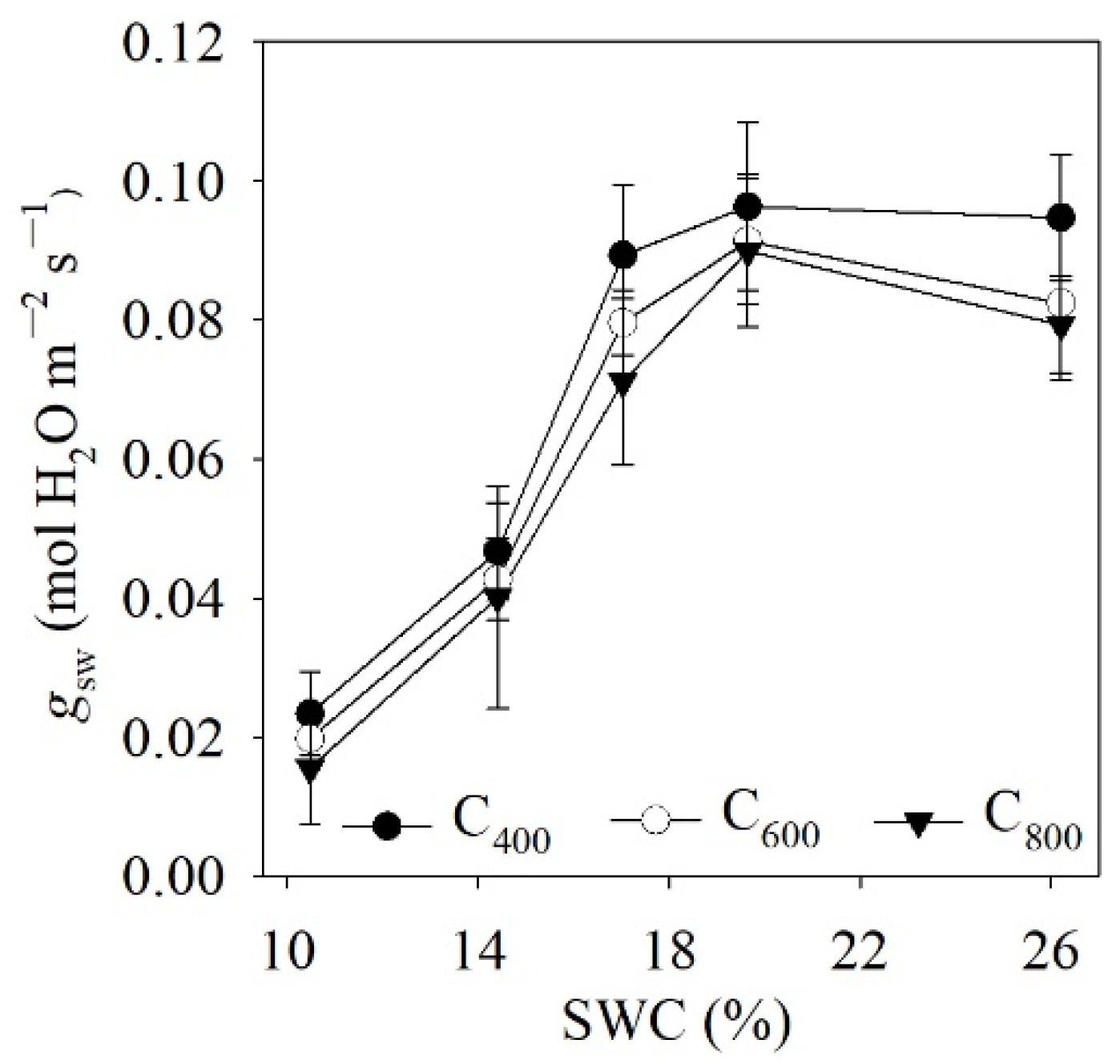
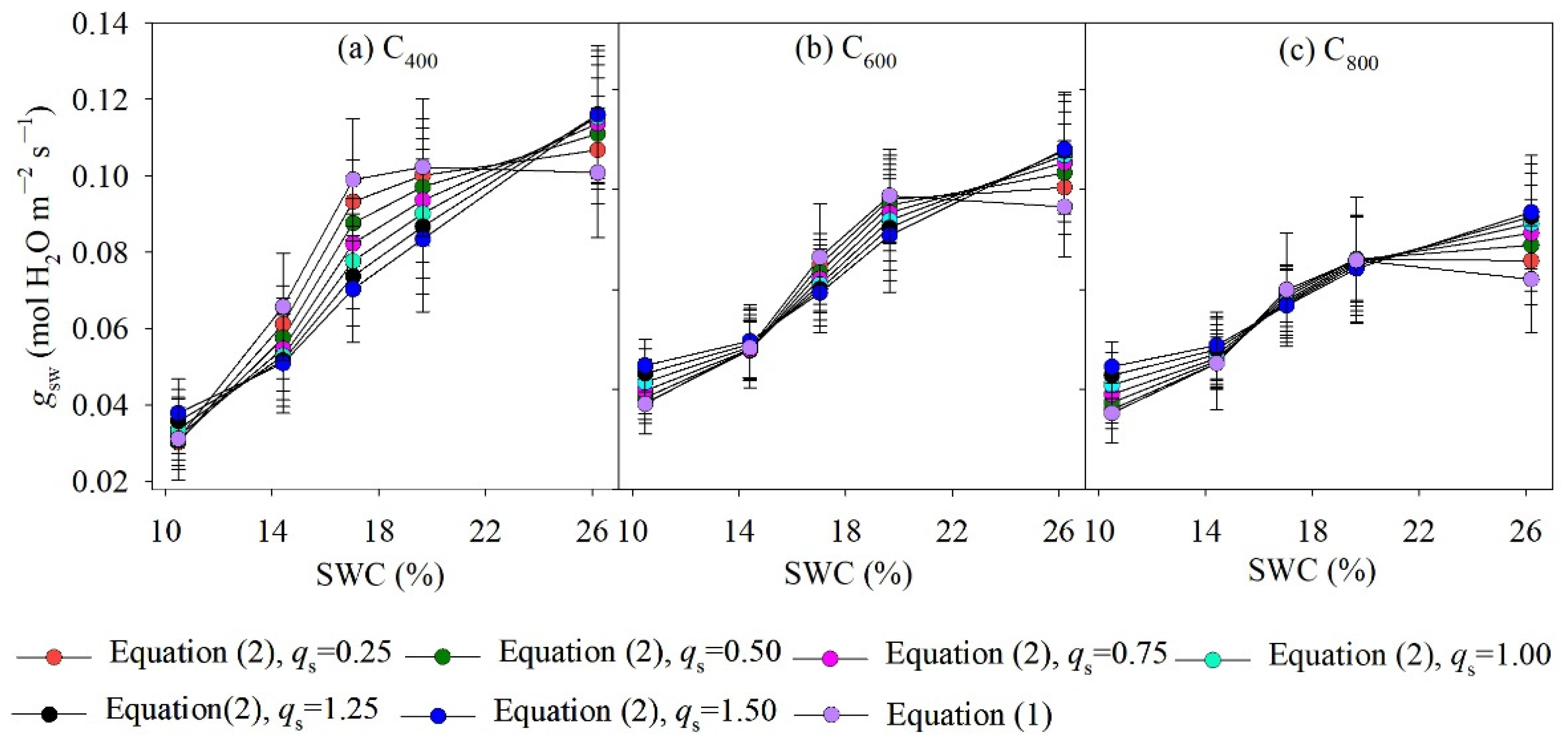
4.1. Measured and Modelled Responses of g_sw to SWC and C_a

Changes in SWC and C_a significantly affected g_sw (p < 0.05), with a maximum of 0.0963 mmol H₂O·m⁻²·s⁻¹ at C₄₀₀ × 19.65% of SWC and a minimum of 0.0155 mol H₂O·m⁻²·s⁻¹ at C₈₀₀ × 10.48% of SWC (Figure 2). In all cases, g_sw decreased with elevated C_a. The g_sw increased sharply as water stress was alleviated irrespective of C_a, and this effect was less evident when SWC exceeded 17.03% and even decreased when g_sw peaked at 19.65% of SWC (Figure 2).

The g_sw simulated by the two coupled P_n,L-g_sw model (Equations (1) and (2)) decreased in response to elevated C_a (Figure 3). In the absence of additional parameterization associated with soil water stress (Equation (1)), the g_sw increased as the soil water status improved and reached maximum values at 19.65% of SWC, with a slight decrease thereafter. In contrast, when the effect of soil water stress was incorporated in the coupled P_n,L-g_sw model (Equation (2)), the simulated g_sw generally increased as SWC increased, regardless of the value imposed by q_s (Figure 3).

The correlation between the measured and calculated g_sw is shown in

Table 1. Correlation analysis between measured and modeled leaf stomatal conductance (g_sw, mol H₂O·m⁻²·s⁻¹) using different models (Equations (1) and (2)).

Model	Regression of Measured and Modelled Leaf gsw
	Linear Regression Equation	R2	p
Equation (2), qs = 0.25	y = 0.88x + 0.01	0.88	<0.01
Equation (2), qs = 0.50	y = 0.86x + 0.01	0.86	<0.01
Equation (2), qs = 0.75	y = 0.83x + 0.01	0.83	<0.01
Equation (2), qs = 1.00	y = 0.79x + 0.01	0.79	<0.01
Equation (2), qs = 1.25	y = 0.74x + 0.02	0.74	<0.01
Equation (2), qs = 1.50	y = 0.68x + 0.02	0.68	<0.01
Equation (1)	y = 0.87x + 0.01	0.87	<0.01

. When applying Equation (2), we found a strong correlation between the calculated and the measured g_sw (p < 0.01), and the correlation coefficient R² decreased from 0.88 to 0.68 as q_s increased from 0.25 to 1.50. The calculated g_sw based on Equation (1) also significantly correlated with the measured g_sw (p < 0.01; R² = 0.87). However, when applying Equation (2), at q_s = 0.25, the calculated g_sw (higher R² and slope closer to (1) was closer to measured g_sw than when using Equation (1). Additionally, with Equation (2), there was less deviation (0.0084 ± 0.0053 mol H₂O·m⁻²·s⁻¹) between the measured and calculated g_sw than with Equation (1) (0.0086 ± 0.0062 mol H₂O·m⁻²·s⁻¹). This showed that the P_n,L–g_sw model, which incorporates the soil water stress (q_s = 0.25, Equation (2)), better predicts g_sw than Equation (1).

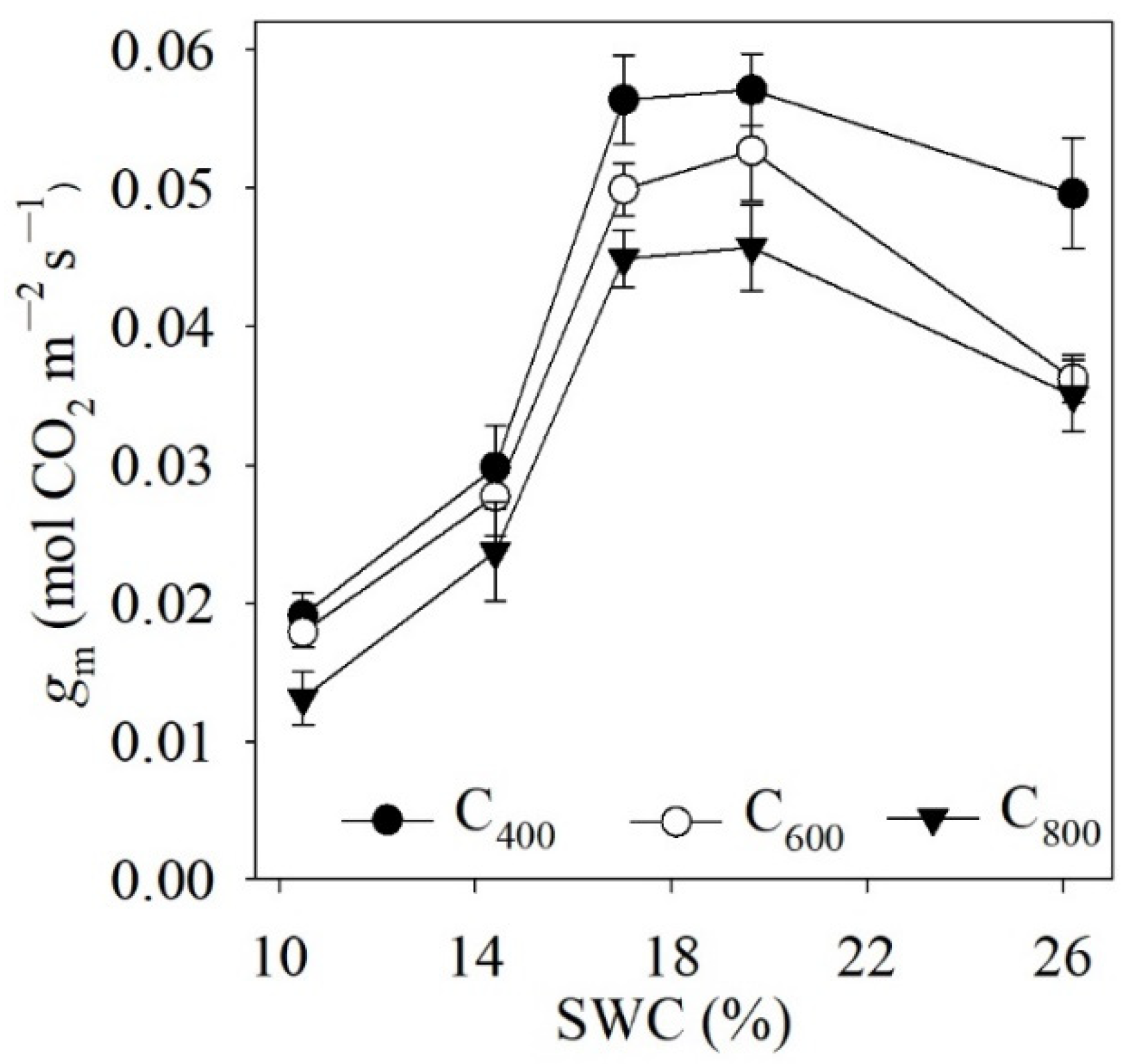
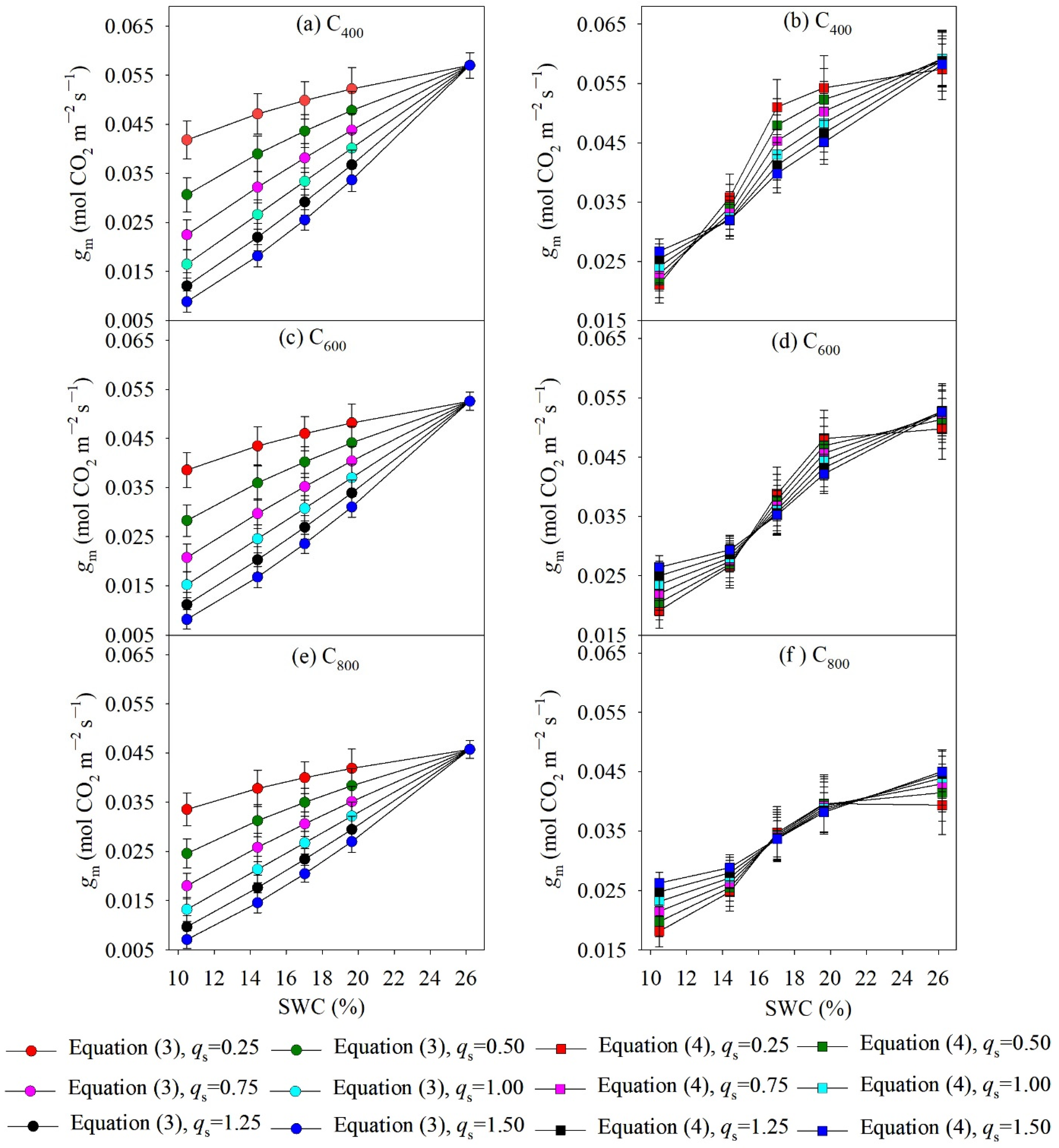
4.2. Measured and Modelled Responses of g_m to SWC and C_a

The g_m ranged between 0.0131 and 0.0571 mol CO₂·m⁻²·s⁻¹, significantly lower than g_sw (p < 0.05). Elevation of C_a produced significant changes in g_m. In all case, elevated C_a decreased g_m (Figure 4). Additionally, SWC significantly influenced the g_m (p < 0.05) in a similar pattern as g_sw. Under low soil moisture content, g_m increased rapidly with SWC. However, the rate of increase in g_m decreased when SWC exceeded 17.03% and even decreased at SWC between 19.65% and 25.55% (Figure 4).

The simulated g_m, calculated by the SWC- and g_m,0-dependent function (Equation (3)) and the coupled P_n,L-g_m model (Equation (4)), is presented in Figure 5. Regardless of the model used, the calculated g_m decreased with C_a (Figure 5). Applying Equation (3), the simulated g_m increased almost linearly with an increase in SWC levels and tended to be higher with lower q_m, except under excess SWC (25.55% of SWC) (Figure 5a,c,e). In contrast, the simulated g_m calculated by Equation (4), using various q_m values, produced a more complicated tendency to SWC. (Figure 5b,d,f).

The relationships between measured and calculated g_m based on Equations (3) and (4) are shown in

Table 2. Correlation analysis between measured and modeled leaf mesophyll conductance (g_m, mol CO₂·m⁻²·s⁻¹) using different models (Equations (3) and (4)).

Model	Regression of Measured and Modeled Leaf gsw
	Linear Regression Equation	R2	p
Equation (3), qm = 0.25	y = 0.30x + 0.03	0.50	<0.01
Equation (3), qm = 0.50	y = 0.44x + 0.02	0.52	<0.01
Equation (3), qm = 0.75	y = 0.53x + 0.02	0.48	<0.05
Equation (3), qm = 1.00	y = 0.58x + 0.01	0.43	<0.05
Equation (3), qm = 1.25	y = 0.61x + 0.01	0.38	<0.05
Equation (3), qm = 1.50	y = 0.61x + 0.03	0.34	<0.05
Equation (3), qm = 0.25	y = 0.79x + 0.01	0.79	<0.01
Equation (3), qm = 0.50	y = 0.72x + 0.01	0.72	<0.01
Equation (3), qm = 0.75	y = 0.65x + 0.01	0.65	<0.01
Equation (3), qm = 1.00	y = 0.57x + 0.02	0.57	<0.01
Equation (3), qm = 1.25	y = 0.51x + 0.02	0.51	<0.01
Equation (3), qm = 1.50	y = 0.44x + 0.02	0.44	<0.01

. Both model approaches produced significant relationships between simulated and measured results (p < 0.05). Setting the same q_m value, Equation (4) led to a higher R² (0.44 ~ 0.79) between the estimated and measured results than that of Equation (3) (0.34 ~ 0.52), and the former caused less deviation (0.0055 ± 0.0038 ~ 0.0097 ± 0.0046) from measurements than the latter (0.0090 ± 0.0058 ~ 0.0159 ± 0.0078). Therefore, the proposed coupled P_n,L-g_m model with well parameterized q_m (q_m = 0.25, Equation (4)) effectively improved the predictive accuracy of g_m compared to the previously introduced g_m,p- and SWC-dependent model (Equation (3)).

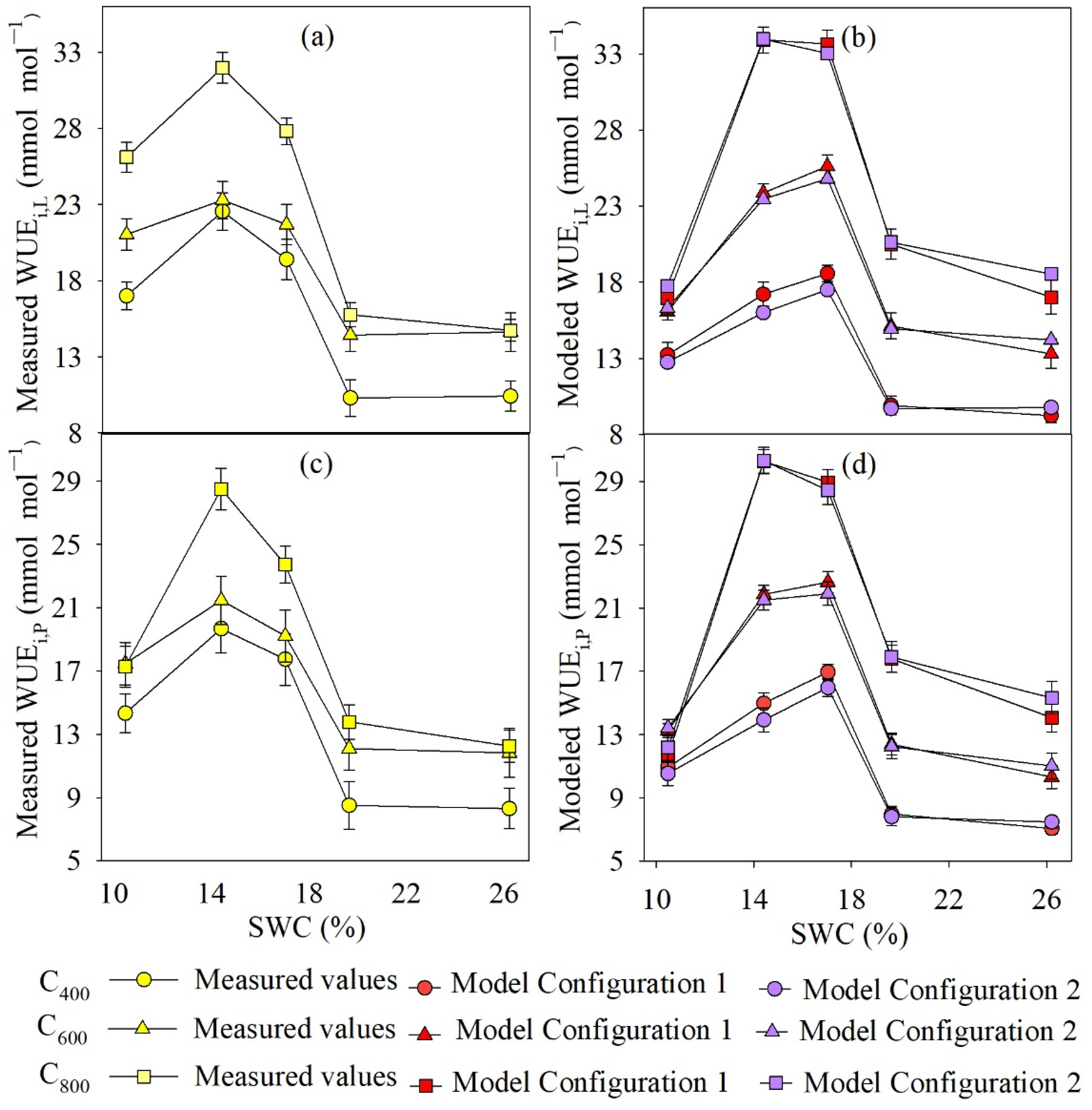
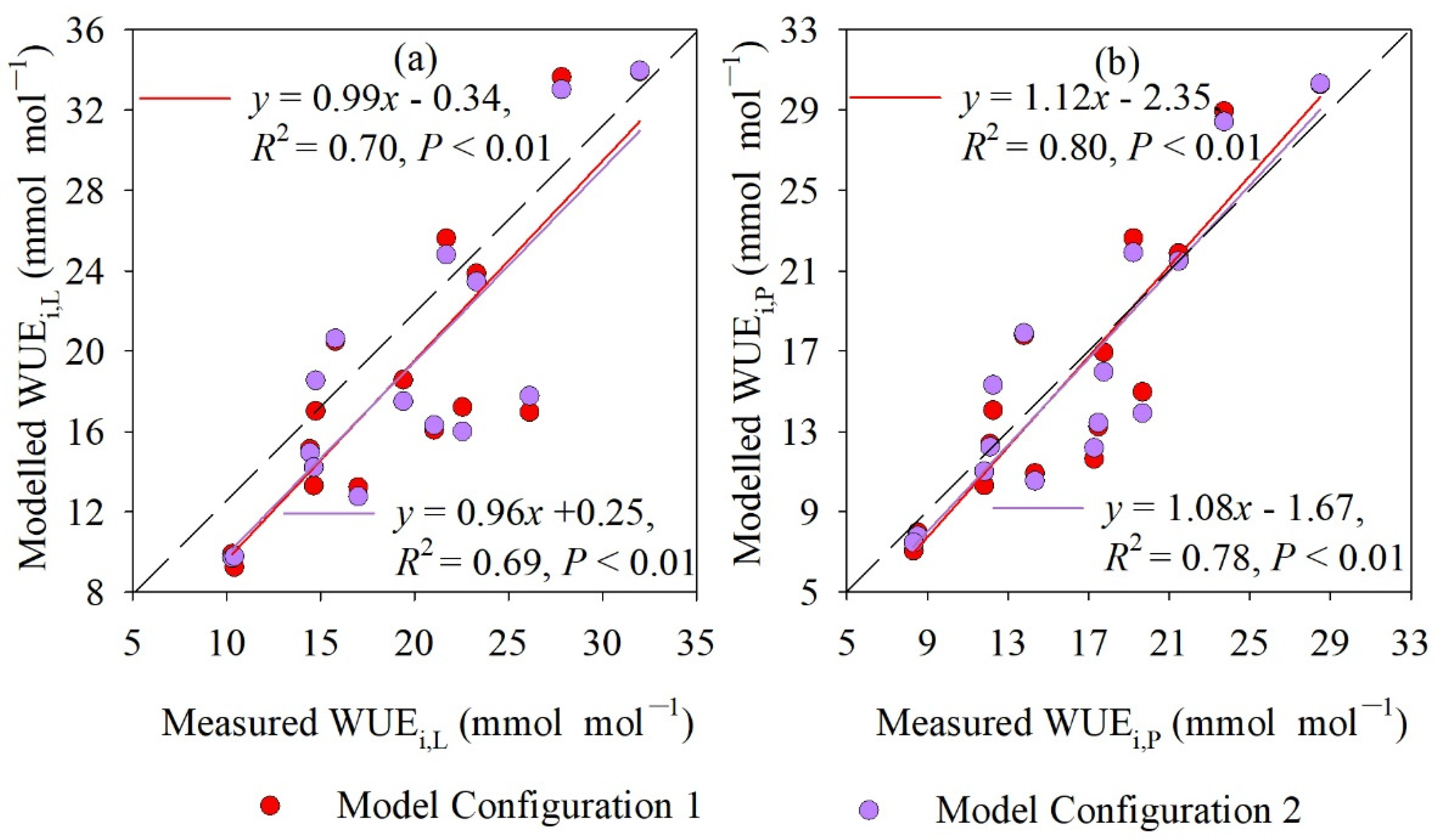
4.3. Measured and Modeled Instantaneous WUE at Leaf and Whole-Plant Level

At the leaf level, elevated C_a significantly enhanced the measured WUE_i,L (p < 0.05). Variations in SWC also significantly influenced the measured WUE_i,L (p < 0.05), which increased as the severe drought was alleviated (SWC increased from 10.48% to 14.41%), followed by a decline with increasing SWC levels and was almost constant when the SWC was above 19.65% (Figure 6a). In both model configurations, the response pattern of simulated WUE_i,L to SWC × C_a was similar to that of measured values, except that the simulated WUE_i,L increased as the SWC improved from 14.41 to 17.03% at C₄₀₀ and C₆₀₀, departing from the observed decreasing trend (Figure 6a,b).

At the whole-plant level, it was observed that C_a and SWC significantly influenced (p < 0.05) the measured instantaneous WUE (WUE_i,P). In general, the measured WUE_i,P was higher at elevated C_a levels (Figure 6c). When the SWC increased from 10.48% to 14.41%, the percentage increase in the measured WUE_i,P was more pronounced at C₈₀₀ than at C₄₀₀ and C₆₀₀. In response to further increases in SWC, the measured WUE_i,P generally decreased sharply with further rises in SWC, but this trend was lesser when the soil water status was more than 19.65% of SWC. In both model configurations, the measured and simulated WUE_i,P values were similar in their response patterns to SWC × C_a, except when the SWC increased from 14.41% to 17.03% at C₄₀₀ and C₆₀₀ (Figure 6c,d).

At the leaf and whole-plant level, both models revealed a strong correlation between the measured and calculated instantaneous WUE (p < 0.01). However, the relationship was stronger for model configuration 1 (C1), relative to model configuration 2 (C2) (Figure 7). In C1, the calculated WUE_i,L (WUE_i,P) deviated from measured WUE_i,L by 3.12 ± 2.44 (2.59 ± 1.86) mmol·mol⁻¹, which was slightly less than that realized with C2 (3.14 ± 2.52 (2.62 ± 1.90) mmol·mol⁻¹ (Figure 7). This indicates that C1 was more accurate than C2 in predicting WUE_i,L and WUE_i,P.

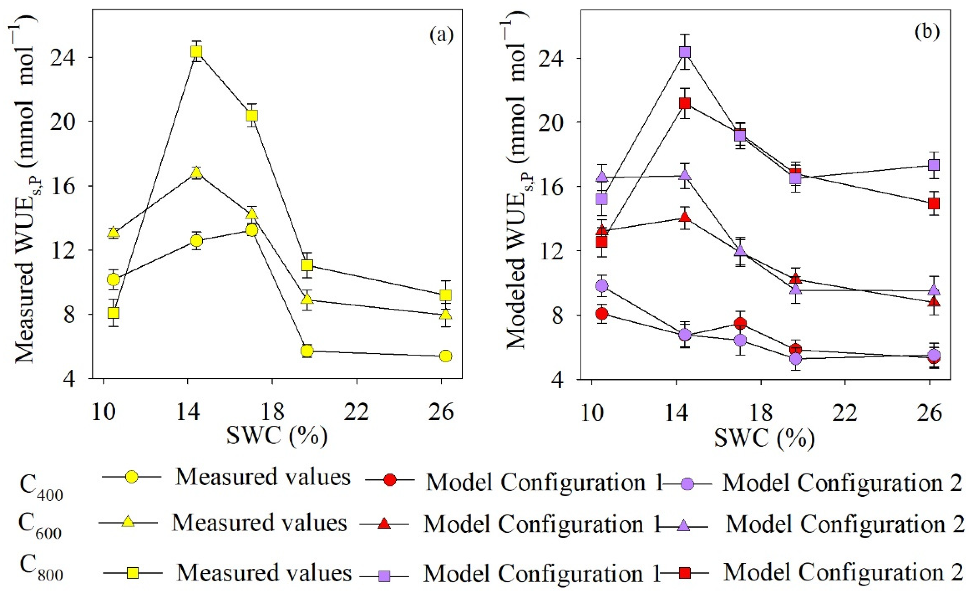
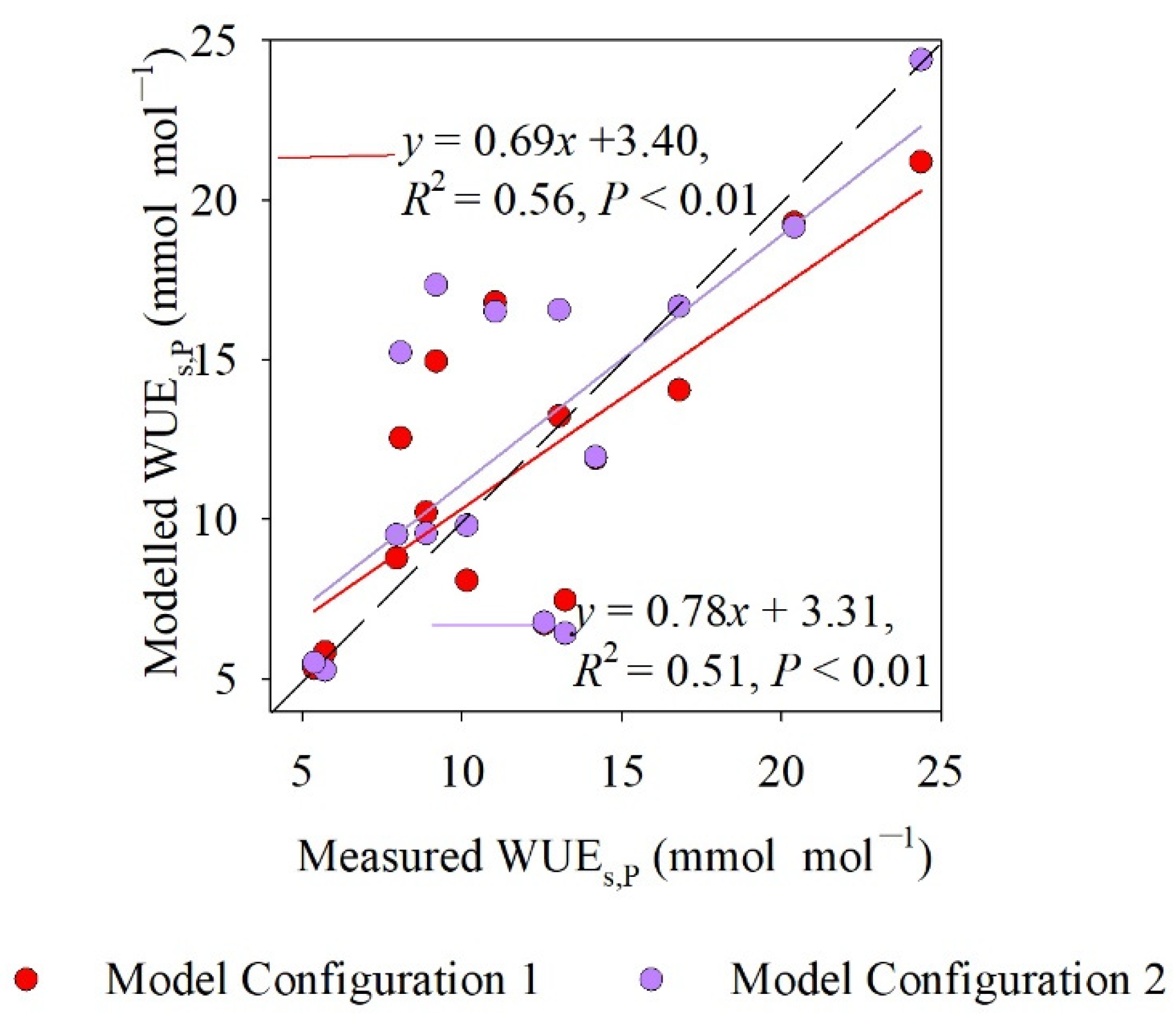
4.4. Comparison of Measured and Modeled WUE_s,P Values

The measured and simulated WUE_s,P values are shown in Figure 8. At severe drought (10.48% of SWC), the measured WUE_s,P peaked at C₆₀₀ and was lowest at C₈₀₀, whereas the simulated WUE_s,P, in both model configurations, reached its maximum at C₆₀₀ and was lowest at C₄₀₀ (Figure 8). At an improved soil water status (SWC at 14.41% ~ 25.55%), the measured and simulated WUE_s,P values significantly increased due to elevated C_a levels (p < 0.01). The measured WUE_s,P was also significantly influenced by SWC, generally responding in a similar manner as the measured WUE_i,P in response to SWC. When the saplings were subjected to SWC of 14.41% ~ 25.55%, in C1, the response pattern of simulated WUE_s,P to SWC was consistent with that of the measured values. In contrast, in C2, the simulated WUE_s,P increased as the SWC increased from 19.65 to 26.20% under any C_a, which differed from the response pattern of the measured values (Figure 8).

In both model configurations, there was a strong correlation between the measured and calculated WUE_s,P (p < 0.01). However, the correlation (R²) was stronger for the C1 model, relative to the C2 model (Figure 9). In the C1 model, the calculated WUE_s,P deviated from measured WUE_s,P by 2.77 ± 2.23 mmol·mol⁻¹, compared with 2.91 ± 2.95 mmol·mol⁻¹ for the C2 model (Figure 9). Therefore, compared with C2, C1 better predicts the actual WUE_s,P.

5. Discussion

5.1. Model Performance for Estimating g_sw and g_m

Soil water stress exclusion in the coupled P_n,L-g_sw model (Equation (1)) for response patterns of g_sw performed reasonably well under non-limiting soil water conditions (Table 1), which is in agreement with previous studies conducted in almond trees [22] and in maize and soybean plants [21]. In response to contrasting soil water treatments, the combination of a soil moisture-dependent function with the coupled P_n,L-g_sw model (Equation (2)) using well parameterized q_s (0.25), was slightly more capable of representing the observed pattern of g_sw than Equation (1). These results align with a previous study, which highlights the importance of including the water stress function in the coupled P_n,L-g_sw model [35]. However, adding the soil water stress-dependent function to the coupled P_n,L-g_sw model contributed little to the improvement of model performance for g_sw. This can be ascribed to the fact that the measured P_n,L incorporated the effect of the soil water status, resulting in the estimation of g_sw from the coupled A_n-g_sw model accounting for the effect of soil water.

The Keenan et al. (2010) [12] model (Equation (3)) for g_m was insufficient to take into account the impact of C_a and was therefore less suitable to simulate g_m (Table 2). In contrast, the predictive accuracy improved considerably when estimating g_m using the coupled P_n,L-g_m model (Equation (4)). Therefore, the proposed coupled P_n,L-g_m model is valid and promising for simulating g_m, despite its phenomenological nature and dependence on physiological hypotheses. Furthermore, imposing q_m = 0.25 in Equation (4) provided the best fit with the measured values (Figure 6), indicating that the limitation strength of g_m was similar to that of g_sw. This result conflicts with the general findings that stomatal behaviour imposed a higher limitation on photosynthesis than mesophyll behavior [22,36,37]. However, such a phenomenon may not always occur. For example, Pérez-Martín et al. (2009) [4] observed minor difference between stomatal and mesophyll limitations and reported that stiffer and more sclerophyllous leaves would provide greater mesophyll resistance during CO₂ diffusion.

In addition, this study found that, mostly, g_sw (and g_m) values varied with SWC, even if the influence of C_a on g_sw (and g_m) was significant. Centritto et al. (2002) [38] also found that g_sw was significantly lower in water-stressed seedlings than in well-watered seedlings, while elevated C_a did not significantly influence g_sw under either well-watered or water-stressed conditions. However, Flexas et al. (2007) [24] observed that both g_sw and g_m were much higher in 400 µmol·mol⁻¹ air than those in 1000 µmol·mol⁻¹ air. Thus, C_a effects on g_sw (or even g_m) may not be universal across species.

5.2. Different Model Configurations for Estimating WUE_s,P

In our proposed short-term WUE model (Equation (15)), scaling up from the leaf to the whole-plant level, there are diffusive limitation parameters. The C1 inferred from Equations (2) and (4) could more accurately represent the observed WUE_s,P than the C2 inferred from Equations (1) and (3) (Figure 9). This leads us to infer that the model scaling up from the leaf to whole-plant level, based on more accurate stomatal and mesophyll behaviour predictions, could be used to estimate WUE_s,P with a high level of precision. In addition, the developed model for estimating WUE_s,P also contains photosynthetic parameters by introducing the coupled P_n,L-g_sw and P_n,L-g_m models. Rather than estimating P_n,L via the photosynthesis model [21,39], the estimates of WUE_s,P were calculated from measured P_n,L values to exclude the situation that errors in the representation of g_sw and g_m might be compensated or overwhelmed by errors in simulated P_n,L. In such a situation, we can identify the influence of precision of stomatal and mesophyll modelling on the credibility and accuracy of the developed WUE_s,P model.

For WUE_i,L and WUE_i,P modelling, the C1 inferred from the more accurate g_sw model incorporating a soil water stress-dependent function (Equation (2)) slightly outperformed the C2 (Figure 7a,b). However, the R² between measured and modelled WUE_s,P were lower than those of WUE_i,L and WUE_i-P (Figure 7 and Figure 9), most likely because the involvement of more parameters in the isotope-inferred WUE_s,P model could introduce more uncertainties and errors. For example, complications arising from post-photosynthetic carbon isotope fractionations are not considered as the process is still difficult to assess and largely unknown [40,41]. Furthermore, the effects of photorespiration and mitochondrial respiration on photosynthetic ¹³C discrimination are still the subject of debate [25] and were thus ignored in the current study.

5.3. Uncertainties of WUE_s,P Introduced by g_sw and g_m

Uncertainty analysis was conducted to further determine the uncertainties of WUE_s,P associated with stomatal and mesophyll behaviour simulations. Using the most effective approach to reproduce g_sw (Equation (2), with tunable parameter q_s = 0.25) and g_m (Equation (4), with tunable parameter q_m = 0.25), the average uncertainties (s.d.) in g_sw and g_m were 17.10% (14.14%) and 15.39% (10.98%), respectively. The WUE_s,P estimated from C1 caused average uncertainties (s.d.) of 24.09% (21.61%). The relatively small discrepancies between mean value and standard deviation in uncertainties of g_sw, g_m, and WUE_s,P indicate that these estimation methods were not stable, although model performance was improved. In addition, the WUE_s,P was more sensitive to g_sw than to g_m. That is, 10% error in g_sw introduced 6.17% error in WUE_s,P, while 10% error in g_m introduced a smaller error of 4.48% in WUE_s,P. Although the stomatal and mesophyll limitations were similar to those of the photosynthetic process in this study, the leaf transpiration is exclusively controlled by g_sw when the v is almost constant [9,10,42] (Seibt et al., 2008; Zhao et al., 2017; Zhang et al., 2019), which could result in the g_sw being a more influential factor for WUE_s,P than the g_m.

Overall, the explored whole-plant model, based on well-characterized coupled P_n,L-g_sw (Equation (2)) and P_n,L-g_m models (Equation (4)), is applicable for evaluating variation in WUE_s,P in response to C_a and SWC. However, we recognize that Platycladus orientalis is a very specific plant, and the results are hard to generalize for all other plants. It is therefore important to collect data from different plants to further examine the model. In addition, using only data of pot-grown saplings acclimated in growth chambers, with relatively similar canopy components (canopy structure, light interception), is not convincing enough for a general verification of the developed modelling approach. For field-grown plants with a complex canopy structure, water potential and gas exchange information for individual leaves cannot be consistent for the whole-plant level [43,44], leading to difficulties in generalizing the estimation of WUE_s,P from leaf properties. Moreover, root systems have been excluded from gas exchange measurements due to it being impossible to separate root and soil respiration for technical restriction. In conclusion, the ability of the whole-plant model to simulate WUE_s,P features should still be explored and improved.

6. Conclusions

In this study, the performances of coupled P_n,L-g_sw and P_n,L-g_m models were evaluated using leaf gas exchange measurements. We found the coupled P_n,L–g_sw model incorporating the water stress-dependent function with well parameterized q_s (Equation (2)) agreed slightly better with the measured g_sw values than the model excluding the soil water stress effect (Equation (1)), and the established coupled P_n,L-g_m model with well parameterized q_m (Equation (4)) allowed for a more reliable estimation of g_m than the previously introduced g_m,p- and SWC-dependent model (Equation (3)). Based on the well-characterized models describing stomatal and mesophyll behavior, an isotopic model, scaling from the leaf to whole-plant level for estimating WUE_s,P (Equation (16)), was then established and validated. We found the developed model for WUE_s,P proved effective at capturing response patterns to C_a and SWC. Therefore, introducing the model performing well for g_sw and g_m into the Farquhar et al. (1989) model was applicable and represents a promising approach for describing whole-plant WUE at smaller temporal scales.

References

1. Medrano, H.; Tomás, M.; Martorell, S.; Flexas, J.; Hernández, E.; Rosselló, J.; Pou, A.; Escalona, J.-M.; Bota, J. From leaf to whole–plant water use efficiency WUE in complex canopies: Limitations of leaf WUE as a selection target. Crop J. 2015, 3, 220–228. [Google Scholar] [CrossRef] [Green Version]
2. Flexas, J.; Ribas-Carbó, M.; Bota, J.; Galmés, J.; Henkle, M.; Martínez-Cañellas, S.; Medrano, H. Decreased Rubisco activity during water stress is not induced by decreased relative water content but related to conditions of low stomatal conductance and chloroplast CO2 concentration. New Phytol. 2006, 172, 73–82. [Google Scholar] [CrossRef]
3. Warren, C.R.; Adams, M.A. Internal conductance does not scale with photosynthetic capacity, implications for carbon isotope discrimination and the economics of water and nitrogen use in photosynthesis. Plant Cell Environ. 2006, 29, 192–201. [Google Scholar] [CrossRef] [PubMed]
4. Perez-Martin, A.; Flexas, J.; Ribas-Carbo, M.; Bota, J.; Tomas, M.S.; Infante, J.M.; Diaz-Espejo, A. Interactive effects of soil water deficit and air vapour pressure deficit on mesophyll conductance to CO2 in Vitis vinifera and Olea europaea. J. Exp. Bot. 2009, 60, 2391–2405. [Google Scholar] [CrossRef]
5. Hu, J.; Moore DJ, P.; Riveros-Iregui, D.A.; Burns, S.P.; Monson, R.K. Modeling whole–tree carbon assimilation rate using observed transpiration rates and needle sugar carbon isotope ratios. New Phytol. 2010, 1854, 1000–1015. [Google Scholar] [CrossRef] [PubMed] [Green Version]
6. Farquhar, G.D.; Richards, R.A. Isotopic composition of plant carbon correlates with water–use efficiency in wheat genotypes. Aust. J. Plant Physiol. 1984, 11, 539–552. [Google Scholar] [CrossRef]
7. Farquhar, G.D.; Ehleringer, J.R.; Hubick, K.T. Carbon isotope discrimination and photosynthesis. Annu. Rev. Plant Physiol. Plant Mol. Biol. 1989, 40, 503–537. [Google Scholar] [CrossRef]
8. Hubick, K.T.; Farquhar, G.D. Carbon isotope discrimination and the ratio of carbon gained to water lost in barley cultivars. Plant Cell Environ. 1989, 12, 795–804. [Google Scholar] [CrossRef]
9. Seibt, U.; Rajabi, A.; Griffiths, H.; Berry, J.A. Carbon isotopes and water–use efficiency, sense and sensitivity. Oecologia 2008, 155, 441–454. [Google Scholar] [CrossRef]
10. Zhang, Y.E.; Yu, X.; Chen, L.; Jia, G. Whole–plant instantaneous and short–term water–use efficiency in response to soil water content and CO2 concentration. Plant Soil 2019, 444, 281–298. [Google Scholar] [CrossRef]
11. Pons, T.L.; Flexas, J.; Von Caemmerer, S.; Evans, J.R.; Genty, B.; Ribas-Carbo, M.; Brugnoli, E. Estimating mesophyll conductance to CO2, methodology potential errors and recommendations. J. Exp. Bot. 2009, 608, 2217–2234. [Google Scholar] [CrossRef] [Green Version]
12. Keenan, T.; Sabate, S.; Gracia, C. Soil water stress and coupled photosynthesis conductance models: Bridging the gap between conflicting reports on the relative roles of stomatal, mesophyll conductance and biochemical limitations to photosynthesis. Agric. For. Meteorol. 2010, 150, 443–453. [Google Scholar] [CrossRef]
13. WMO Greenhouse Gas Bulletin The State of Greenhouse Gases in the Atmosphere Based on Global Observations through 2020; World Meteorological Organization: Geneva, Switzerland, 2021.
14. Ball, J.T.; Woodrow, I.E.; Berry, J.A. A model predicting stomatal conductance and its contribution to the control of photosynthesis under different environmental conditions. In Progress in Photosynthesis Research; Martinus Nijhoff Publishers: Leiden, The Netherlands, 1987. [Google Scholar]
15. Jarvis, P.G. The interpretation of the variations in leaf water potential and stomatal conductance found in canopies in the field. Philos. Trans. R. Soc. B Biol. Sci. 1976, 273, 593–610. [Google Scholar]
16. Leuning, R. Modelling Stomatal Behaviour and and Photosynthesis of Eucalyptus grandis. Funct. Plant Biol. 1990, 17, 159–175. [Google Scholar] [CrossRef]
17. Leuning, R. A critical appraisal of a combined stomatal–photosynthesis model for C3 plants. Plant Cell Environ. 1995, 18, 339–355. [Google Scholar] [CrossRef]
18. Collatz, G.J.; Ball, J.T.; Grivet, C.; Berry, J.A. Physiological and environmental regulation of stomatal conductance, photosynthesis and transpiration: A model that includes a laminar boundary layer. Agric. For. Meteorol. 1991, 54, 107–136. [Google Scholar] [CrossRef]
19. Lloyd, J. Modelling Stomatal Responses to Environment in Macadamia integrifolia. Funct. Plant Biol. 1991, 18, 649–660. [Google Scholar] [CrossRef]
20. Lohammar, T.; Larsson, S.; Linder, S.; Falk, S.O. FAST: Simulation Models of Gaseous Exchange in Scots Pine. Ecol. Bull. 1980, 32, 505–523. [Google Scholar]
21. Yu, G.R.; Zhuang, J.; Yu, Z.L. An attempt to establish a synthetic model of photosynthesis–transpiration based on stomatal behavior for maize and soybean plants grown in field. Plant Physiol. 2001, 158, 861–874. [Google Scholar] [CrossRef]
22. Egea, G.; Verhoef, A.; González–Real, M.M.; Baille, A.; Nortes, P.A.; Domingo, R. Comparison of several approaches to modelling stomatal conductance in well–watered and drought–stressed almond trees. Acta Hortic. 2011, 922, 285–293. [Google Scholar] [CrossRef]
23. Egea, G.; Verhoef, A.; Vidale, P.L. Towards an improved and more flexible representation of water stress in coupled photosynthesis–stomatal conductance models. Agric. For. Meteorol. 2011, 151, 1370–1384. [Google Scholar] [CrossRef]
24. Flexas, J.; Diaz-Espejo, A.; Galmés, J.; Kaldenhoff, R.; Medrano, H.; Ribas-Carbo, M. Rapid variations of mesophyll conductance in response to changes in CO2 concentration around leaves. Plant Cell Environ. 2007, 30, 1284–1298. [Google Scholar] [CrossRef] [PubMed]
25. Douthe, C.; Dreyer, E.; Brendel, O.; Warren, C.R. Is mesophyll conductance to CO2 in leaves of three Eucalyptus species sensitive to short–term changes of irradiance under ambient as well as low O2? Funct. Plant Biol. 2012, 38, 434–447. [Google Scholar] [CrossRef]
26. Misson, L.; Limousin, J.M.; Rodriguez, R.; Letts, M.G. Leaf physiological responses to extreme droughts in Mediterranean Quercus ilex forest. Plant Cell Environ. 2010, 33, 1898–1910. [Google Scholar] [CrossRef] [PubMed]
27. Xu, Z.; Zhou, G. Responses of photosynthetic capacity to soil moisture gradient in perennial rhizome grass and perennial bunchgrass. BMC Plant Biol. 2011, 11, 21. [Google Scholar] [CrossRef] [PubMed] [Green Version]
28. Porporato, A.; Laio, F.; Ridolfi, L.; Rodriguez-Iturbe, I. Plants in water–controlled ecosystems: Active role in hydrologic processes and response to water stress Ⅲ. Vegetation water stress. Adv. Water Resour. 2001, 24, 725–744. [Google Scholar] [CrossRef]
29. Gessler, A.; Rennenberg, H.; Keitel, C. Stable isotope composition of organic compounds transported in the phloem of European beech–evaluation of different methods of phloem sap collection and assessment of gradients in carbon isotope composition during leaf–to–stem transport. Plant Biol. 2004, 6, 721–729. [Google Scholar] [CrossRef]
30. Hu, J.; Moore DJ, P.; Monson, R.K. Weather and climate controls over the seasonal carbon isotope dynamics of sugars from subalpine forest trees. Plant Cell Environ. 2009, 33, 35–47. [Google Scholar] [CrossRef]
31. Kodama, N.; Barnard, R.L.; Salmon, Y.; Weston, C.; Ferrio, J.P.; Holst, J.; Gessler, A. Temporal dynamics of the carbon isotope composition in a Pinus sylvestris stand: From newly assimilated organic carbon to respired carbon dioxide. Oecologia 2008, 156, 737–750. [Google Scholar] [CrossRef] [PubMed]
32. Jasoni, R.; Kane, C.; Green, C.; Peffley, E.; Tissue, D.; Thompson, L.; Payton, P.; Paré, P.W. Altered leaf and root emissions from onion (Allium cepa L.) grown under elevated CO2 conditions. Environ. Exp. Bot. 2004, 51, 273–280. [Google Scholar] [CrossRef]
33. Escalona, J.M.; Fuentes, S.; Tomás, M.; Martorell, S.; Flexas, J.; Medrano, H. Responses of leaf night transpiration to drought stress in Vitis vinifera L. Agric. Water Manag. 2013, 118, 50–58. [Google Scholar] [CrossRef]
34. Farquhar, G.D.; O’Leary, M.H.; Berry, J.A. On the relationship between carbon isotope discrimination and the intercellular carbon dioxide concentration in leaves. Aust. J. Plant Physiol. 1982, 9, 121–137. [Google Scholar] [CrossRef]
35. Sala, A.; Tenhunen, J.D. Simulations of canopy net photosynthesis and transpiration in Quercus ilex L under the influence of seasonal drought. Agric. For. Meteorol. 1996, 78, 203–222. [Google Scholar] [CrossRef]
36. Galmés, J.; Medrano, H.; Flexas, J. Photosynthetic limitations in response to water stress and recovery in Mediterranean plants with different growth forms. New Phytol. 2007, 175, 81–93. [Google Scholar] [CrossRef] [PubMed]
37. Grassi, G.; Magnani, F. Stomatal, mesophyll conductance and biochemical limitations to photosynthesis as affected by drought and leaf ontogeny in ash and oak trees. Plant Cell Environ. 2005, 28, 834–849. [Google Scholar] [CrossRef]
38. Centritto, M.; Lucas, M.E.; Jarvis, P.G. Gas exchange, biomass, whole-plant water-use efficiency and water uptake of peach (Prunus persica) seedlings in response to elevated carbon dioxide concentration and water availability. Tree Physiol. 2002, 22, 699–706. [Google Scholar] [CrossRef] [PubMed]
39. Jones, H.G. Plants and Microclimate, 2nd ed.; Cambridge University Press: New York, NY, USA, 1992; pp. 163–214. [Google Scholar]
40. Tcherkez, G.; Cornic, G.; Bligny, R.; Gout, E.; Ghashghaie, J. In Vivo Respiratory Metabolism of Illuminated Leaves. Plant Physiol. 2005, 138, 1596–1606. [Google Scholar] [CrossRef] [Green Version]
41. Wingate, L.; Seibt, U.; Moncrieff, J.B.; Jarvis, P.G.; Lloyd, J. Variations in 13C discrimination during CO2 exchange by Picea sitchensis branches in the field. Plant Cell Environ. 2007, 30, 600–616. [Google Scholar] [CrossRef]
42. Zhao, N.; Meng, P.; He, Y.B.; Yu, X. Interaction of CO2 concentrations and water stress in semiarid plants causes diverging response in instantaneous win instantaneous water use efficiency and carbon isotope composition. Biogeoscience 2017, 14, 3431–3444. [Google Scholar] [CrossRef] [Green Version]
43. McCutchan, H.; Shackel, K.A. Stem-water Potential as a Sensitive Indicator of Water Stress in Prune Trees (Prunus domestica L. cv. French). J. Am. Soc. Hortic. Sci. 1992, 117, 607–611. [Google Scholar] [CrossRef] [Green Version]
44. Bögelein, R.; Hassdenteufel, M.; Thomas, F.M.; Werner, W. Comparison of leaf gas exchange and stable isotope signature of water-soluble compounds along canopy gradients of co-occurring Douglas-fir and European beech. Plant Cell Environ. 2012, 35, 1245–1257. [Google Scholar] [CrossRef] [PubMed]
Figure 1. Schematic of growth chambers used in the experiments. One growth chamber (a) was used to maintain elevated CO2 concentration of 600 μmol·mol−1 or 800 μmol·mol−1. Another growth chamber (b) was used to maintain CO2 concentration of 400 μmol·mol−1. There were five pots inside each chamber.
Water 14 00263 g001
Figure 2. Response of measured leaf stomatal conductance (gsw, mol H2O·m−2·s−1) to three CO2 concentrations (Ca) × five soil water contents (SWC). C400, C600, and C800 are Ca of 400, 600, and 800 µmol·mol−1. Data represent mean values ± SD.
Water 14 00263 g002
Figure 3. The estimated leaf stomatal conductance (gsw, mol H2O·m−2·s−1) in Platycladus orientalis saplings under different soil water contents (SWC) and CO2 concentrations (Ca) conditions, based on different models (Equations (1) and (2)). C400, C600, and C800 are Ca of 400 (a), 600 (b), and 800 µmol·mol−1 (c). Tunable parameter qs is a measure of the nonlinearity of the effects of soil water stress on the stomatal limiting mechanisms. Data represent mean values ± SD.
Water 14 00263 g003
Figure 4. Response of measured leaf mesophyll conductance (gm, mol CO2·m−2·s−1) to three CO2 concentrations (Ca) × five soil water contents (SWC). C400, C600, and C800 are Ca of 400, 600, and 800 µmol·mol−1. Data represent mean values ± SD.
Water 14 00263 g004
Figure 5. The estimated leaf mesophyll conductance (gm, mol CO2·m−2·s−1) is based on different models (Equation (3), (a,c,e); and Equation (4), (b,d,f) under varying soil water contents (SWC) and CO2 concentrations (Ca). C400, C600, and C800 are Ca of 400 (a,b), 600 (c,d), and 800 µmol·mol−1 (e,f). Tunable parameter qm is a measure of the nonlinearity of the effects of soil water stress on the mesophyll limiting mechanisms. Data represent mean values ± SD.
Water 14 00263 g005
Figure 6. Measured (a) and simulated (b) leaf water use efficiency (WUEi-L, mmol·mol−1), and measured (c) and simulated (d) whole-plant level instantaneous water use efficiency (WUEi-P, mmol·mol−1) in different model configurations under five soil water contents (SWC) × three CO2 concentrations (Ca) conditions. C400, C600, and C800 are Ca of 400, 600, and 800 µmol·mol−1. Data represent mean values ± SD.
Water 14 00263 g006
Figure 7. Correlation analysis between measured and modeled results of leaf instantaneous water use efficiency (WUEi-L, mmol·mol−1) estimated by different model configurations (a), as well as between measured and modeled results of whole-plant instantaneous water use efficiency (WUEi-P, mmol·mol−1) estimated by different model configurations (b).
Water 14 00263 g007
Figure 8. Measured (a) and modelled (b) whole-plant short-term water use efficiency (WUEs,P, mmol·mol−1) under five soil water contents (SWC) × three CO2 concentrations (Ca) conditions. C400, C600, and C800 are Ca of 400, 600, and 800 µmol·mol−1. Data represent mean values ± SD.
Water 14 00263 g008
Figure 9. Correlation analysis between measured and modeled whole-plant short-term water use efficiency (WUEs,P, mmol·mol−1) estimated by different model configurations.
Water 14 00263 g009