
A Data Assimilation Approach to the Modeling of 3D Hydrodynamic Flow Velocity in River Reaches
1
Hydrology and Water Resources Department, Nanjing Hydraulic Research Institute, Nanjing 210029, China
2
Nanjing Automation Institute of Water Conservancy and Hydrology, Ministry of Water Resources, Nanjing 210012, China
3
Heilongjiang Provincial River Basin Management and Guarantee Center, Harbin 150046, China
*
Author to whom correspondence should be addressed.
Water 2022, 14(22), 3598; https://doi.org/10.3390/w14223598
Submission received: 22 September 2022
/
Revised: 27 October 2022
/
Accepted: 3 November 2022
/
Published: 8 November 2022
(This article belongs to the Section Hydraulics and Hydrodynamics)
Abstract
:The measurement of river discharge is essential for sustainable water resource management. The velocity–area approach is the most common method for calculating river discharge. Although several velocity measurement methods exist, they often have varying degrees of technical issues attributed to their operational complexity, time effectiveness, accuracy, and environmental impact. To address these issues, we propose a three-dimensional (3D) hydrodynamic model coupled with data assimilation (DA) for velocity measurement with improved accuracy and efficiency. We then apply this model to the Lanxi River reach in Zhejiang Province, China. The experimental results confirm that the obtained assimilated velocities using our proposed algorithm are much closer to the observed velocities than the simulated velocities. Our results show that when using the proposed method, the RMSE is decreased by 78%, and the SKILL and DASS values are 0.96 and 0.92, respectively. These confirm that the DA scheme of the flow velocity measurement is effective and capable of significantly improving the accuracy of the velocity with lower computational complexity.
1. Introduction
Flow velocity is an essential hydrological factor used to evaluate discharge through the velocity–area method [1]. Therefore, an accurate flow velocity is a prerequisite for obtaining an accurate discharge estimation, which is the base for developing flood control techniques, water supply systems, and agricultural and energy production. Pariva et al. [2] reviewed the existing methods for measuring flow velocity and investigated their pros and cons (Table 1). Several flow velocity measurement techniques exist. For instance, the float method is a low-cost and straightforward method. However, its accuracy is limited. An alternative is the dilution gauging method, which also has low accuracy and further affects the environment. The trajectory method requires expert and trained manpower and complex calculations [3].
Another flow velocity measurement technique is the current meter method. This method, however, is challenging to implement and labor-intensive, and hence it is only suitable for short-term studies [4,5]. Moreover, the effectiveness of horizontal acoustic Doppler current profilers (HADCP) is influenced by blind spots near the river boundaries. Surface velocity radar, as another example, is highly dependent on the roughness of the river surface and can be affected by the existing environmental noises [6]. Large-scale particle image velocimetry (LSPIV) is also used for measurement. To establish a geometric transformation of the digital images, LSPIV requires sufficient ground reference points in the field of view. Therefore, in cases where the reference points are covered by flood water, LSPIV accuracy is significantly reduced [7].
We argue that a three-dimensional (3D) hydrodynamic model coupled with data assimilation (DA) addresses the above issues of the existing current velocity measurement methods and further improves the accuracy and efficiency of velocity measurement. The 3D hydrodynamic model provides information about the distribution of and variation in the flow velocity during the simulation period. Then, DA offers the best estimation of the model state variables by combining the dynamic model and actual data [8,9,10] to ensure that the dynamic model does not deviate from reality.
Several previous works also considered utilizing real data to improve numerical models. For instance, the 3D hydrodynamic model was used by Akiko et al. (2015) to investigate the dispersion of suspended matter in Lake Sakylan Pyhajarvi. In their work, they derived turbidity from satellite data and then analyzed the applicability of direct insertion of the total suspended matter (TSM) concentration field into the numerical model. It was then shown that direct insertion significantly improves the forecast, even if it is applied occasionally [11]. Nowicki et al. (2016) developed an automatic monitoring system to forecast the physical and ecological changes and control the conditions and bio-productivity of the Baltic sea environment. Similarly, in their proposed approach, satellite-measured data assimilation was adopted to constrain the eco-hydrodynamic model, where they reported improvement in accuracy [12].
Furthermore, Wang et al. (2019) developed a fully integrated catchment-wide modeling and monitoring framework based on the 3D hydrodynamic water quality model and DA. They then applied their approach to real-time forecasting and made long-term predictions for water quality [13]. Theo et al. (2020) also proposed a flexible framework incorporating DA into 3D hydrodynamic lake models, where in situ and satellite remote sensing temperature data were assimilated to understand the physical dynamics in the lake ecosystem management. They further showed that DA effectively improves model performance over a broad range of spatiotemporal scales and physical processes, where the temperature error was reduced by 54% [14]. To improve the model results and map local phenomena occurring in the Gulf of Gdansk area, Janecki et al. (2021) also extended the EcoFish numerical model using a satellite data assimilation module. This module assimilated the SST data from a medium-resolution imaging spectroradiometer and an advanced ultrahigh-resolution radiometer, reducing the error, compared with in situ experimental data [15].
Although using a 3D hydrodynamic model coupled with DA to estimate the model state variables is often used in coastal waters and environment management, it has rarely been used in hydrometry. The DA method can assimilate a variety of data (such as point-wise data, vertical-wise data, and data at a certain level of water body) and data types (water level data, velocity data, roughness factor data, and temperature data) into a hydrodynamic model [14,16,17,18]. Due to its flexibility in assimilating data and data types, in areas of hydrometry, it is possible to use this approach to correct the velocity state variables of the 3D hydrodynamic model with a variety of observational data and data types for providing accurate flow velocity values. For example, point-wise velocity data, vertical-wise velocity data, and velocity data at a certain level of water body, water level data, roughness factor data, and other data are used alone or simultaneously to correct velocity state variables of a 3D hydrodynamic model to improve the accuracy and efficiency of velocity measurement. This is an alternative to the current velocity measurement methods.
In this paper, a DA scheme of velocity measurement based on coupling a 3D hydrodynamic model with DA is developed to improve the accuracy and efficiency further. This paper is organized into the following sections: Section 2 describes the proposed approach and presents a practical experiment. Section 3 provides the results and discusses the main findings of the practical experiment. Conclusions are briefly presented in Section 4.
2. Materials and Methods
2.1. TELEMAC System
A hydrodynamic model that can be coupled with DA in a user-friendly manner and allow a variety of data and data types to be inserted in the future with less computation cost will be the first choice for simulating the river reach in this study. The open TELEMAC-MASCARET (www.opentelemac.org, accessed on 13 January 2021) is a non-commercial, open-source numerical suite system, developed by Eletricité de France (EDF) for hydrodynamic numerical simulations. Since its birth (1987), this software by EDF has been continuously serving the energy industry. It has rich user technical support and a wide range of industrial applications and verification and has been approved by safety authorities. It is based on the FORTRAN language and formed by a conjunction of modules in two or three dimensions. This software is widely used to study flows (MASCARET, TELEMAC-2D, and TELEMAC-3D), sediment transport (COURLIS and GAIA), waves (ARTEMIS and TOMAWAC), and water quality (TRACER and WAQTEL) in the coastal and oceanic regions [19,20,21,22,23,24,25]. In this paper, we used the three-dimensional hydrodynamic module TELEMAC-3D. A module using the TELEMAC Application Program Interface (API), the TELAPY module, which is based on Python, was also used in our work. Its open-source nature and user-friendly API facilitate the implementation of the proposed velocity measurement using a 3D hydrodynamic model and DA.
2.1.1. The TELEMAC-3D Model
The TELEMAC-3D model solves the Reynolds-averaged Navier–Stokes equations while incorporating the local variations in the free surface of the fluid. This model further ignores the density variation in the mass conservation equation and considers the hydrostatic pressure and Boussinesq approximation to solve the motion equations. The core of this model is based on the finite element method that solves the hydrodynamic equations. For vertical discretization, this model uses the sigma coordinate system. Further details of model formulations can also be found in [26]. The following three-dimensional equations are solved:
where U, V, and W (m/s) denote the three-dimensional velocity components, p (pa) is the pressure, h (m) denotes the water depth, Zs (m) is the free surface elevation, and Zf (m) denotes the bottom depth. In the above, patm (pa) is the atmospheric pressure, g (m/s2) is the gravitational acceleration, ϑ (m2/s) is the kinematic viscosity and tracer diffusion coefficients, Δρ (kg/m3) is the variation in density around the reference density, t (s) is the simulation time, x and y (m) are the horizontal space components, and z (m) is the vertical space component. U, V, W, and h are the unknown quantities in the above formulations and act as computational variables.
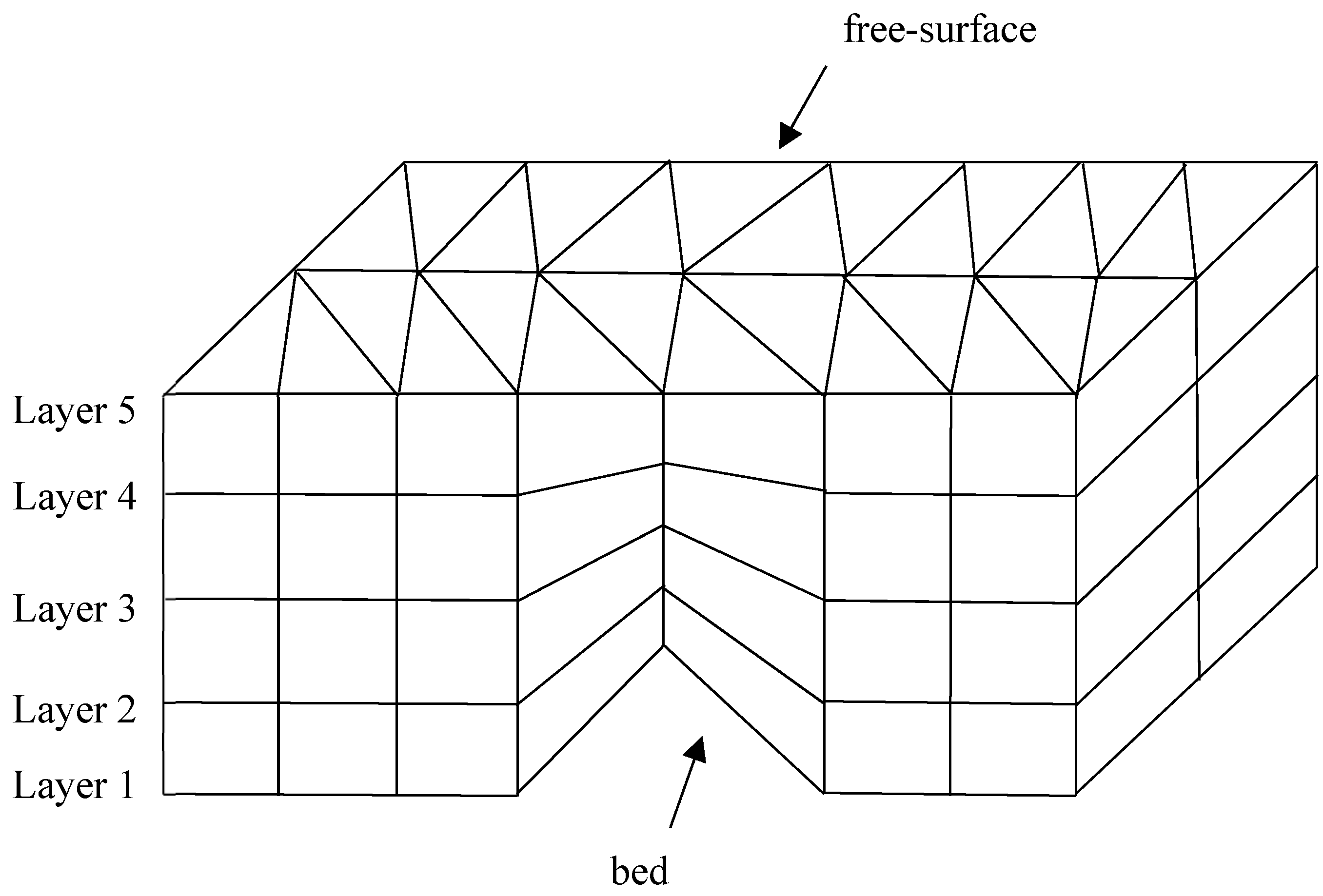
The chosen spatial discretization of the TELEMAC-3D model is a finite element discretization using prisms. Each prism has six nodes with quadrangular vertical sides. The prism with linear interpolation was retained because its two-dimensional (2D) horizontal projection constitutes one of the finite elements (triangle with linear interpolation) used to resolve the Saint–Venant equations in two dimensions. Therefore, to build a 3D mesh, it is possible to build the triangulation of 2D mesh and repeat it along the vertical in superimposed layers [27]. In addition, the elevation of the points belonging to a vertical line should increase from the bed to the free surface (Figure 1). The “superimposed layers” structure of TELEMAC-3D mesh allows the spatial location of a variety of observational data to be accurately and quickly found in the 3D mesh. Moreover, the “superimposed layer” structure of TELEMAC-3D mesh incurs less computation cost than the block-structured mesh of fluid dynamic models, such as OpenFoam, which can also simulate the velocity of the river reach.
2.1.2. The TELAPY Module
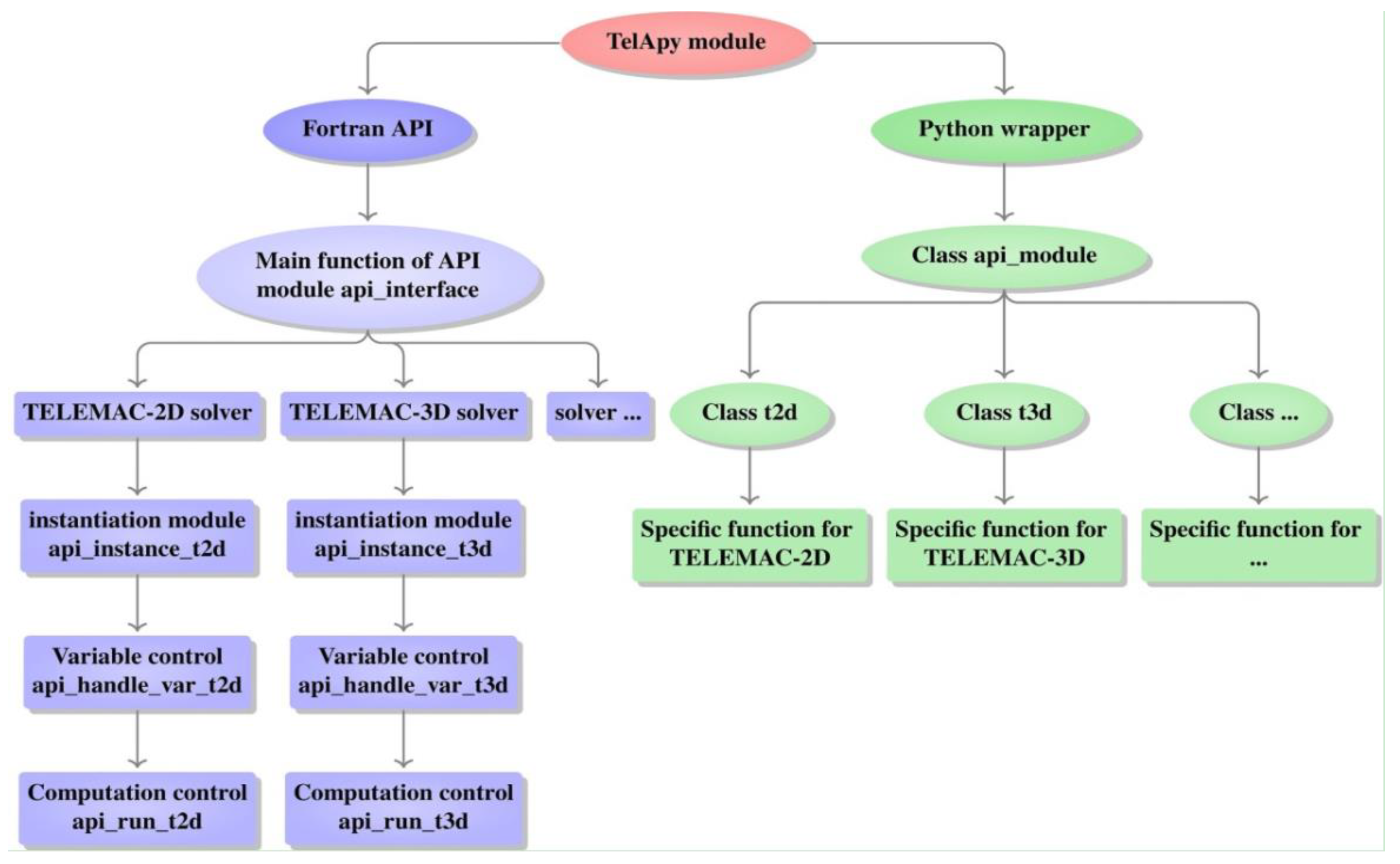
The TELAPY module provides a Python-based interface with the TELEMAC API, where the API controls the simulations [28]. For example, TELAPY enables the user to stop the simulation at any time, retrieve the values of the variables, and modify them. The API is not limited to FORTRAN programming and can be further used by a scripting language, i.e., Python. The details of the TELAPY module are available in [28]. The TELAPY module (Figure 2) also comes with a tutorial that explains controlling the physical components of the TELEMAC-MASCARET SYSTEM in an interactive mode using Python scripting language. API development enables the interoperability of the TELEMAC-MASCARET SYSTEM modules. Interoperability is the ability of a computer system to operate with other existing or future informatic products without restricting access or implementation. This feature enabled coupling the TELEMAC-3D with DA in our work.
2.2. Particle Filter
We used particle filter (PF) as the assimilation algorithm to combine with the TELEMAC-3D model and improve the accuracy of velocity measurements. PF is a sequential Monte Carlo filter, developed based on the sequential importance sampling filter (SIS) of Bayesian sampling estimation [30]. The main idea of PF is to approximate the probability density function (PDF) of the state variables based on random discrete sampling points and replace the integral operation with the sample mean. This is to obtain the minimum variable estimation of the state. These samples are called particles. The PF algorithm consists of the simulation (or prediction) step and the updating (or analysis) step.
- (1)
- The Simulation Step
For N particles, each particle is initialized at time t. There are several methods to initialize the particles. For instance, one may add noise to the state variable(s) or perturb the parameter(s) that critically affect a state variable. In this study, we used the method of adding noise to the velocity variable. The obtained velocity particles are then inserted into the model. The model obtains the particles of the velocity state variable at the next time instant as follows:
where is the velocity state variable analysis value of the particle i at the time t, is the velocity state variable simulated value of the particle i at the time t + 1, represents the relationship of different values of at time t and t + 1 (provided by the TELEMAC-3D model), and is the error that follows a normal distribution with a mean of 0 and a covariance of .
- (2)
- The Updating Step
In the updating step, following the SIS scheme, the weights are updated by the velocity data without changing the particle of the velocity state variable, therefore
In this paper, we used the Gaussian distribution function as the weighting function:
where is the weight of velocity particle i at time t + 1, is the velocity data at time t + 1, is the simulated value of velocity particle i from the simulation step at time t + 1, and is the variance of the velocity particle error.
By increasing the number of filter iterations, the weights of most particles diminish, and only a few particles have a considerable weight. Since particle degeneration is inevitable, resampling becomes an effective way to address this issue. The resampling idea is to inhibit degeneration by resampling particles, where a large number of particles with high weights are kept, and the rest are eliminated. Before resampling, the ordered pair of particles is set, and the weight is . After resampling, the particles with large weights are divided into multiple particles, and particles with minimal weights are discarded. The total number of particles remains the same, and the ordered pair of particles set and weight becomes .
In this paper, we implemented the classical residual resampling method [31] based on multinomial resampling [32]. In the residual resampling method, the normalized weights are multiplied by N, and then the integer value of each weight is applied to define how many samples of that particle are kept. Subtracting the weights by their integer part leaves the fractional part of the number. Multinomial resampling was used to select the rest of the particles based on the residual.
2.3. Practical Experiment
2.3.1. Study Area
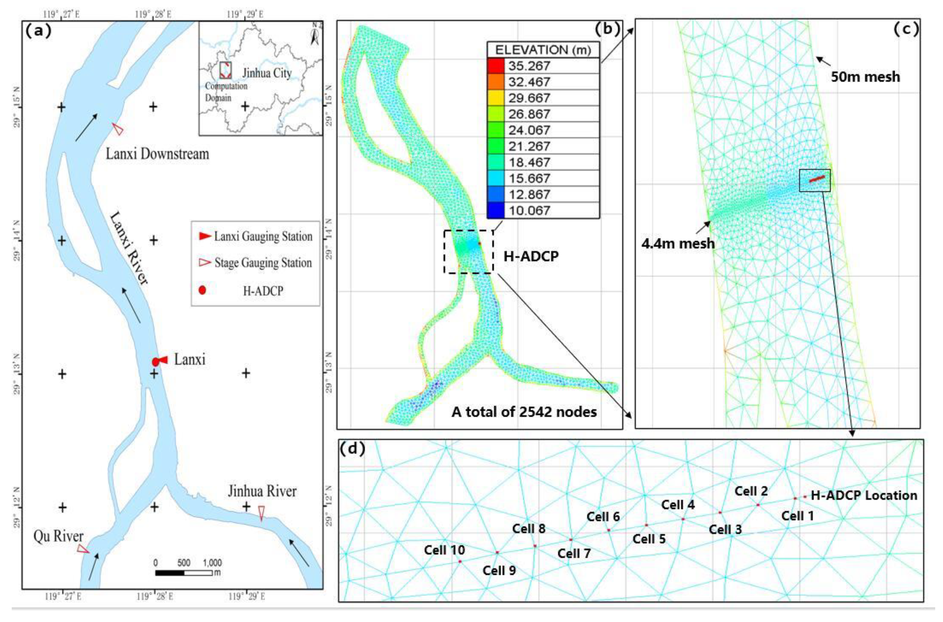
Qiantang River is the largest river in Zhejiang Province, China, where the Lanxi gauging station is the main control station in the midstream. The study area is near the Lanxi gauging station, northwest of Jinhua City, Zhejiang Province. As illustrated in Figure 3a, the experiment’s reach is relatively straight, with 460 m in width and an extension of 7 km. It has a total area of 18,233 km2, and its mean annual river discharge is 544 m3/s. The water flows from the Qu River and Jinhua River into the Lanxi River. Several three-stage gauging stations are set up for the upstream and downstream of the considered experiment to monitor the water level upstream and downstream.
2.3.2. Observations
- 1.
- The water level data
Water level data were gathered from the stage gauging stations on the Qu River, Jinhua River, and Lanxi River in 5 min intervals for 3 days, from 5 January 2022 to 7 January 2022. The water level gauge is a radar water level gauge, and it can measure up to a millimeter (extra fine grade) and is not affected by the water body and environmental factors, such as temperature, humidity, wind speed, and rainfall. The collected data were used as upstream and downstream boundary conditions to establish the 3D hydrodynamic model of the experiment reach using the TELEMAC-3D model.
- 2.
- The flow velocity data
The velocity measurement equipment used in this study is a CM600 horizontal acoustic Doppler current profiler (HADCP) manufactured by the TRDI Company. This equipment also obtains high-quality velocity data for low and unsteady flows that are difficult to measure. CM600 HADCP has an accuracy of 0.5% (0.002 m/s) and a resolution of 0.001 m/s. It was installed below the cable tunnel at an elevation of 0.86 m. It also has a blind spot of 1 m and a total of 10 cells for measuring velocity with a length of 4.4 m for each cell (Figure 3d). The HADCP recorded ensemble-averaged velocity profile data within 5 min intervals from 5 January 2022 to 7 January 2022. The collected data were used to correct the simulated velocity in the reach through the PF algorithm.
2.3.3. TELEMAC-3D Setup
The computation domain was discretized by a non-structured grid of finite elements (triangular elements). The 3D computational grid comprised a 2D grid describing the river bottom geometry duplicated several times along the vertical axis. The 2D finite element grid was composed of 2542 nodes (Figure 3b). The mesh size varied from 4.4 m in the area of HADCP, which was equal to the HADCP cell length, to 50 m (i.e., the computation domain except for the area of HADCP) (Figure 3c). In the TELEMAC-3D model, we used 3 layers, and the height of the middle layer was equal to the HADCP installation elevation. The first layer also represented the bottom reach, and the third layer represented the free surface. This could effectively reduce the computation cost and accurately implement observational data assimilation.
For turbulence modeling, we adopted the common practice of separating the vertical and horizontal turbulence scales that are not relevant to the same dynamics as those used for the standard applications of TELEMAC-3D [33]. This process involves defining horizontal and vertical viscosities rather than a single viscosity. The implementation of TELEMAC-3D, therefore, requires defining two separate models for horizontal and vertical turbulence. To balance the calculation time and quality of results, we chose constant and Prandtl’s mixing length viscosity models for the horizontal and vertical turbulence.
The simulated period of the experiment was from 5 to 7 January 2022, with a simulation time of 1 s. The reach’s upstream and downstream boundary conditions were the time series of the water level data provided by the stage gauging stations at Qu River, Jinhua River, and Lanxi River, respectively. A spin-up of 6 h was also used to generate realistic initial conditions to better simulate the actual reach conditions.
2.3.4. Particle Filter Setup
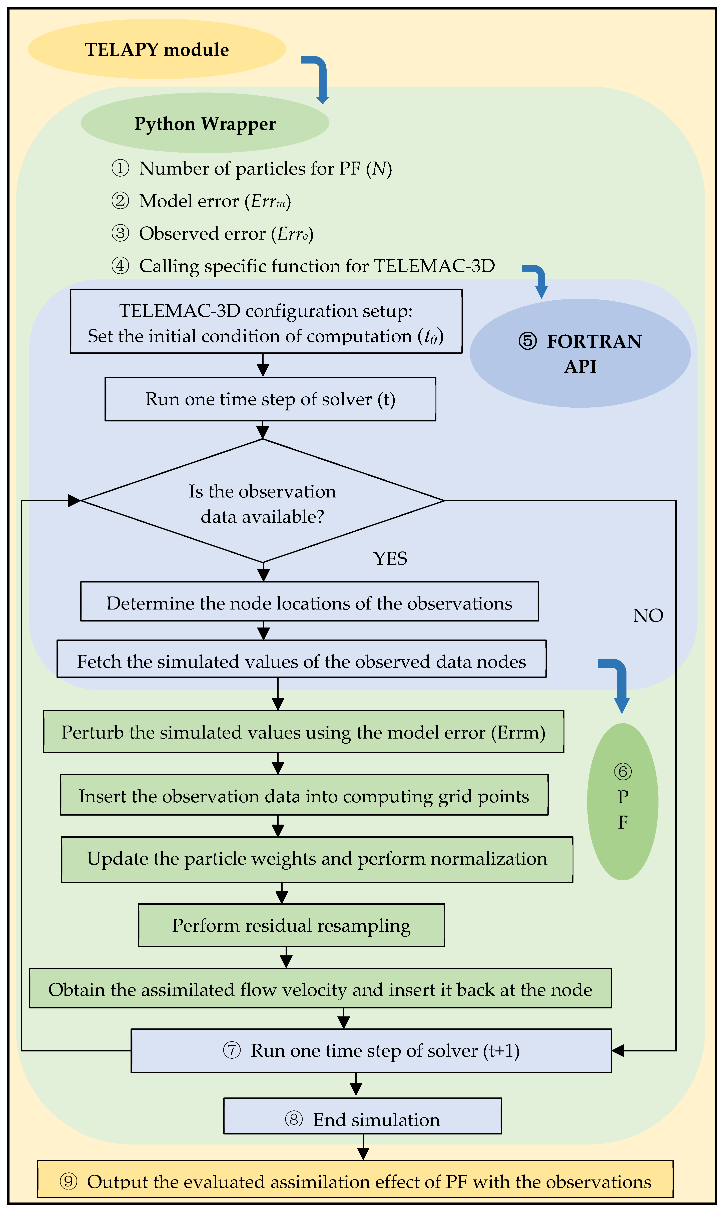
We developed a DA scheme for velocity measurement coupled with the TELEMAC-3D model and PF to improve reliability and efficiency. All processes were performed in the TELAPY module and executed in two phases. In the first phase, each state variable was computed using a specific function in TELEMAC-3D with the FORTRAN API. Then, in the second phase, the state variable particle was updated using the PF algorithm, thus assimilating the HADCP velocity data through the Python Wrapper. The flowchart of the DA scheme is presented in Figure 4. The detailed procedure is described as follows:
- (1)
- (2)
- Call the specific function for TELEMAC-3D from FORTRAN API, then load and initialize the TELEMAC-3D configuration with the computed conditions and start the velocity simulation;
- (3)
- Obtain the velocity state variable at each grid node and each time step;
- (4)
- Determine whether there are observations. If no observations exist, continue the simulation process. Otherwise, determine the locations of the HADCP velocity data according to the HADCP installation elevation (the middle layer of the 3D mesh), the grid resolution (the HADCP cell length of 4.4 m), and the coordinates of HADCP;
- (5)
- Generate the N particles of velocity states in each grid node of the HADCP locations by adding the noises generated by the normal distribution N ~ (0, Errm) at time t;
- (6)
- Add the HADCP velocities in U and V directions;
- (7)
- Compute the weight of each particle and perform normalization according to Equations (6) and (7);
- (8)
- To inhibit particle degeneration, use residual resampling to copy high-weight particles and eliminate low-weight particles based on the weights from the previous step. The new particles contain similar weights;
- (9)
- Obtain the assimilated velocity state variables for each grid node of the HADCP locations and set them as the initial velocities at time t + 1;
- (10)
- Repeat Steps (4)–(9) until the end of the simulation period;
- (11)
- Output the assimilated velocities.
2.4. Model Evaluation
The simulated velocity values were compared with the HADCP velocity data. Three statistical measures, namely the root mean square error (RMSE), the model skill (SKILL), and the data assimilation skill score (DASS), were used for the state variables at each node of the HADCP locations. The mathematical equations of these measures are
where n is the number of timesteps, denotes the simulated value at time i, is the assimilated value at time i, is the observed value at time i, and is the mean of the observed value at time i.
The RMSE is in the range of [0, +∞]. A zero RMSE value means the observed value is consistent with the simulated/assimilated value. The smaller the RMSE value, the higher the accuracy of the simulated/assimilated output.
SKILL is an indicator of model data consistency. A SKILL value of “1” means complete agreement, whereas “0” indicates complete disagreement. Maréchal (2004) [34] showed that the model performance is excellent if SKILL > 0.65, very good if it is between 0.65 and 0.5, good if it is between 0.5 and 0.2, and poor if SKILL < 0.2.
2.5. Model Calibration and Validation
Model calibration is the adjustment of model parameter values within reasonable and acceptable ranges so that the deviations between the model and the measured data are minimized and are within an acceptable range of accuracy. Model validation is the subsequent testing of a calibrated model to a second independent dataset, usually under different external conditions. This is to further examine the model’s ability to represent reality [37] realistically. To evaluate the effect of the PF on the velocity measurements, TELEMAC-3D model calibration and validation had to be performed. The simulation results of the TELEMAC-3D model were compared with the HADCP velocity data at the same time and locations. The performance measures used at this stage were RMSE and SKILL.
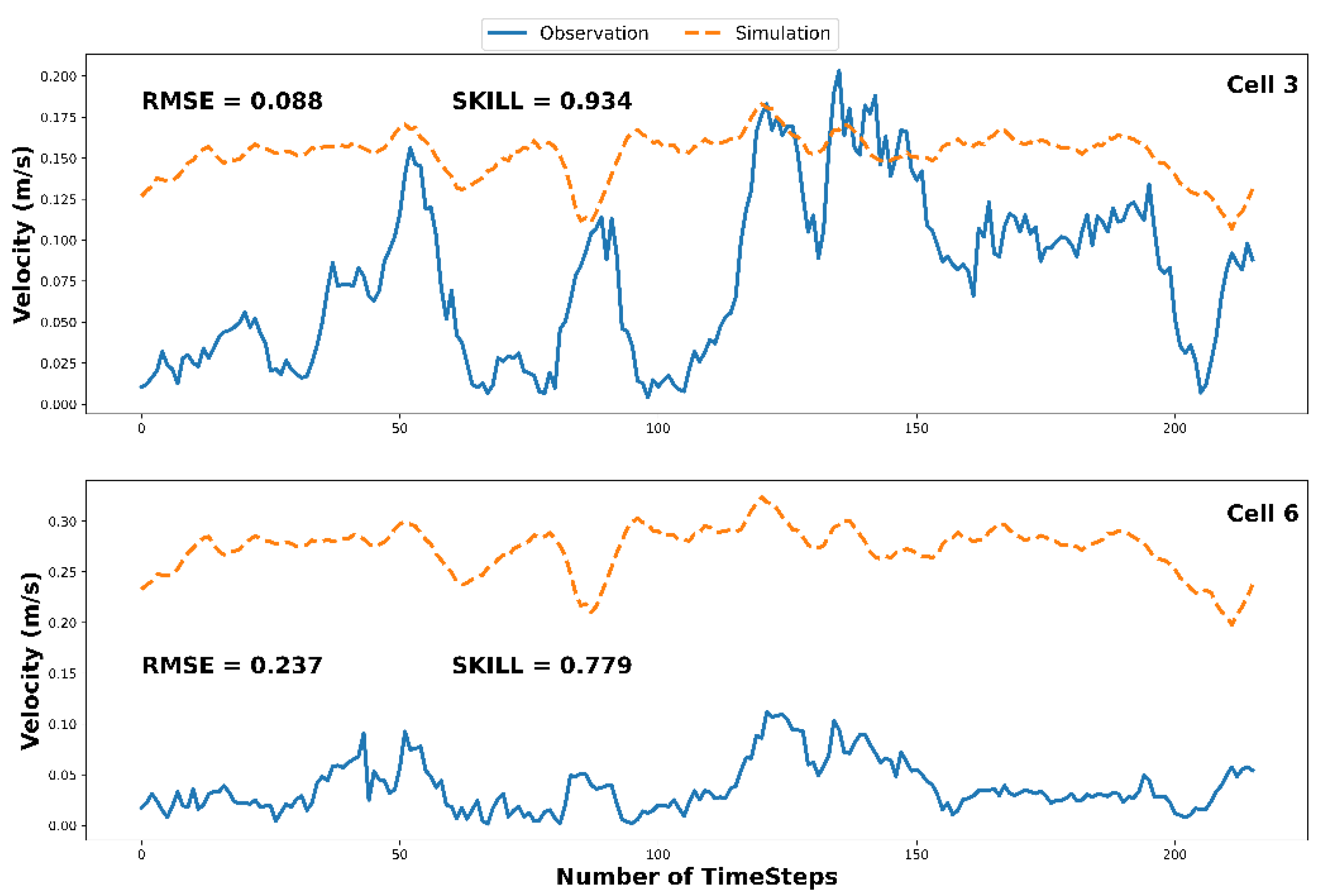
The results of the TELEMAC-3D model calibration exercise are presented in Figure 5, where comparisons between the simulations and the observations are presented within each 5 min interval starting at 06:00 and ending at 23:59 on 5 January 2022, on cells 3 and 6 of the HADCP. The simulated velocity trends of other HADCP cell locations were similar to those in Figure 5. The RMSE and SKILL of the 10 cell locations of the HADCP in the calibration exercise are also shown in Table 2. As seen in the table, the SKILL values ranged from 0.779 to 0.934, with a mean value of 0.86. Therefore, according to the value range of SKILL, the TELEMAC-3D model performance was excellent (0.86 (0.65,1)). However, the model overestimated the velocity, with an RMSE reaching 0.16 m/s (with a range of 0.088–0.237 m/s). This might be attributed to the TELEMAC-3D model settings that balance the computation cost with simulation accuracy.
The mesh size, the superimposed layers, and the choice of the turbulence model affect the simulation accuracy and computation cost. The smaller the mesh size, the higher the simulation accuracy, and the more the computation cost. The computation cost can be reduced by increasing the mesh size appropriately, but the computation convergence should be taken as the premise. In order to accurately find the location of the observed velocity in the computational domain, the 3D mesh was set as a 4.4 m mesh size (the HADCP cell length) over the area of HADCP. To reduce the computation cost and ensure computation convergence, the 50 m mesh size was set in the computation domain except for the area of HADCP.
Similarly, the more superimposed layers, the higher the simulation accuracy, and the longer the calculation time. When the number of superimposed layers is large enough, the calculation time is longer than the simulation period, which makes the simulation meaningless. Therefore, a three-layer of 3D mesh was determined in this study, considering the computational efficiency and effective simulation. Combined with the mesh size and superimposed layers, the spatial location of HADCP velocity data could be quickly and accurately found in the computation domain.
In the choice of the turbulence model, the calculation time and application domain need to be considered. As for the river reach of this study, it is relatively straight, and the flow state of the river reach falls under the general flow state category, which is suitable for a relatively rough turbulence model. Therefore, the constant and Prandtl’s mixing length viscosity models were selected as the horizontal and vertical turbulences for this study because of their small calculation and low-resolution requirement, as well as relative stability and good convergence.
Due to the setting of the mesh size, the superimposed layers, and the turbulence models, the calculation time of this study was controlled within 10 min, while its simulation period was 24 h. This satisfies the need for a high level of time effectiveness in the currently used velocity measurement methods and, therefore, classifies the TELEMAC-3D model’s reproduction as reasonable and acceptable because of the realistic requirement of measuring the velocity.
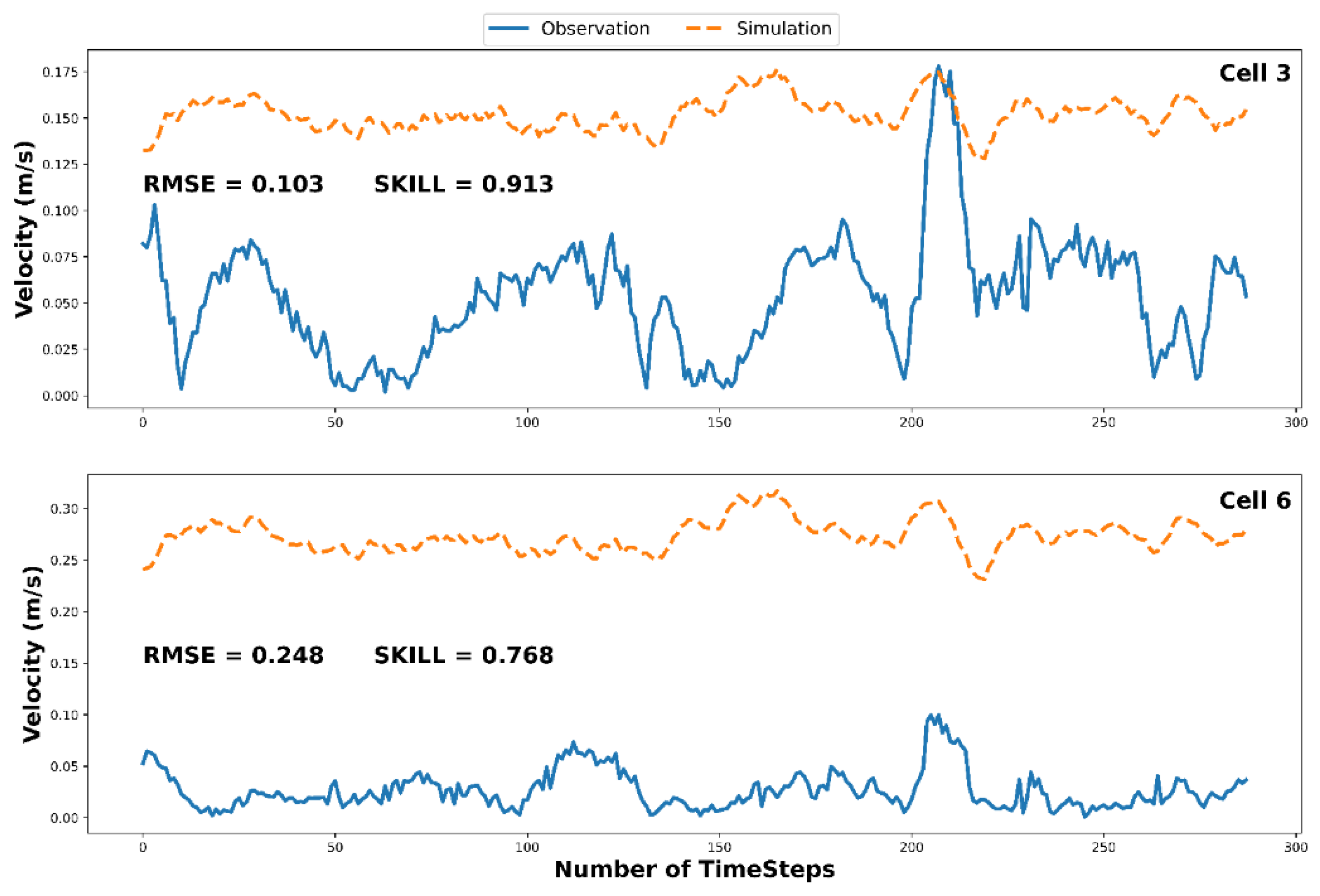
To validate the TELEMAC-3D model, we used the HADCP velocity data within 5 min intervals on 6 January 2022. Figure 6 only displays the simulations and observations in cells 3 and 6 of the HADCP, as the rest followed a similar trend. The details of the RMSE and SKILL results for the 10 cells of the HADCP in the validation exercise are also presented in Table 2. The results were similar to those of the calibration exercise. The mean of the SKILL was 0.84, which showed that the model performance was excellent, while the mean of the RMSE was 0.175 m/s, implying that the model overestimated the velocity. This is the tradeoff between the computation cost and simulation accuracy, considering the realistic requirements of measuring the velocity. Therefore, the validation of the TELEMAC-3D model can be classified as within a reasonable and acceptable range. The above results showed that the TELEMAC-3D model reproduced the velocity of the experiment reach with reasonable and acceptable quality.
3. Results and Discussion
The experiment reach was near Lanxi Gauging Station in Jinhua City, Zhejiang Province, China. In order to simulate the velocity of the experiment reach, the TELEMAC-3D model was established, and the model was performed for calibration and validation. To evaluate the effect of the PF on the velocity measurements, a PF parameter sensitivity analysis was carried out, and in what follows, two treatments, namely the TELEMAC-3D simulation without and with the PF coupling, are discussed and compared.
3.1. Preliminary Sensitivity Analysis
The model error (Errm), observation error (Erro), and the number of particles (N) are essential PF parameters directly affecting the assimilation effectiveness of the PF. To determine the values of these parameters, we performed a sensitivity analysis using the coupled model, and the results are shown in Table 3.
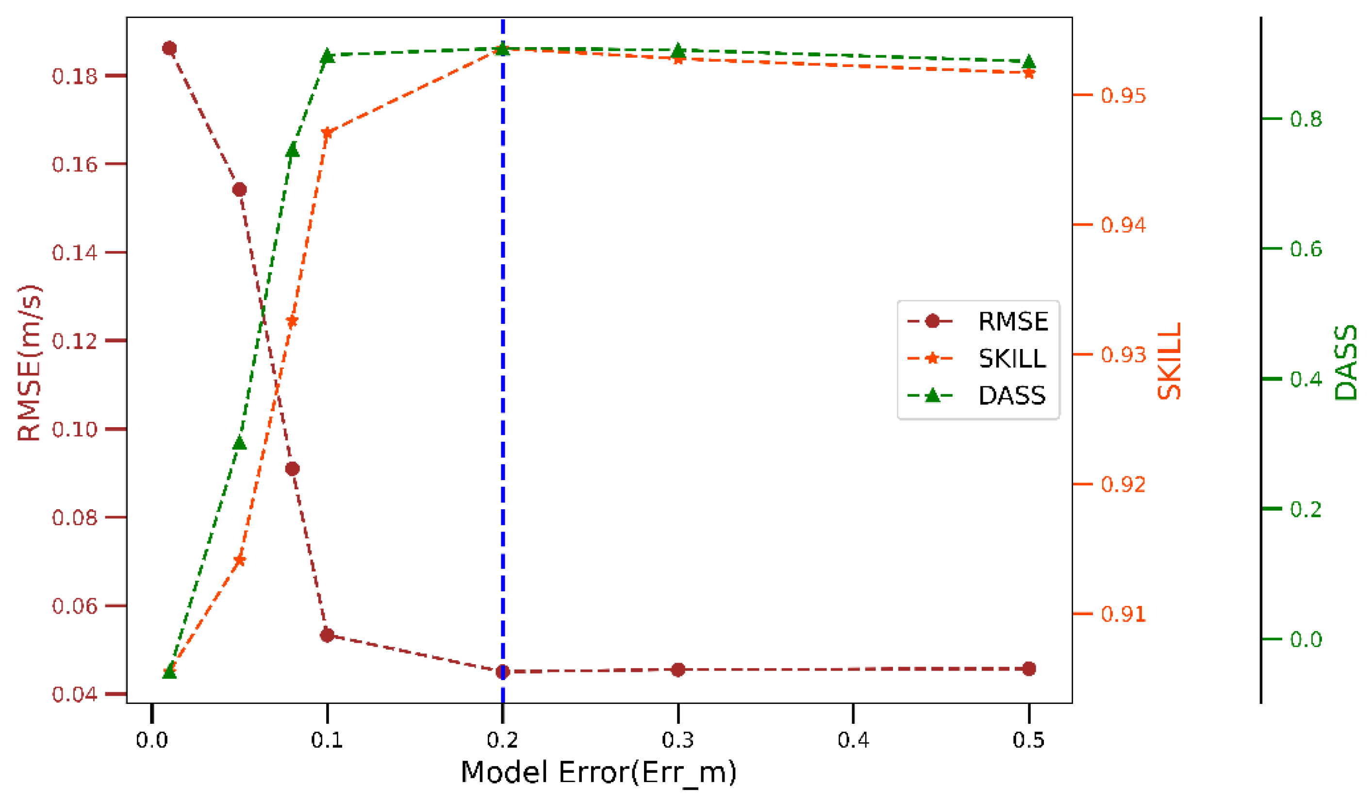
The initial values Errm, Erro, and N, were 0.01, 0.001, and 100, respectively. Figure 7 also illustrates the impact of Errm on the PF. When observation error and number of particles were set to the initial values of 0.001 and 100, respectively, the RMSE of the coupled model was significantly dropped. The values of SKILL and DASS were also significantly increased, with a model error between 0.001 and 0.1. The RMSE value also reached the minimum value (0.045 m/s), and SKILL and DASS had the maximum values of 0.9536 and 0.9077, respectively, with a model error of 0.2. After that, RMSE slightly increased, while SKILL and DASS values were slightly reduced.
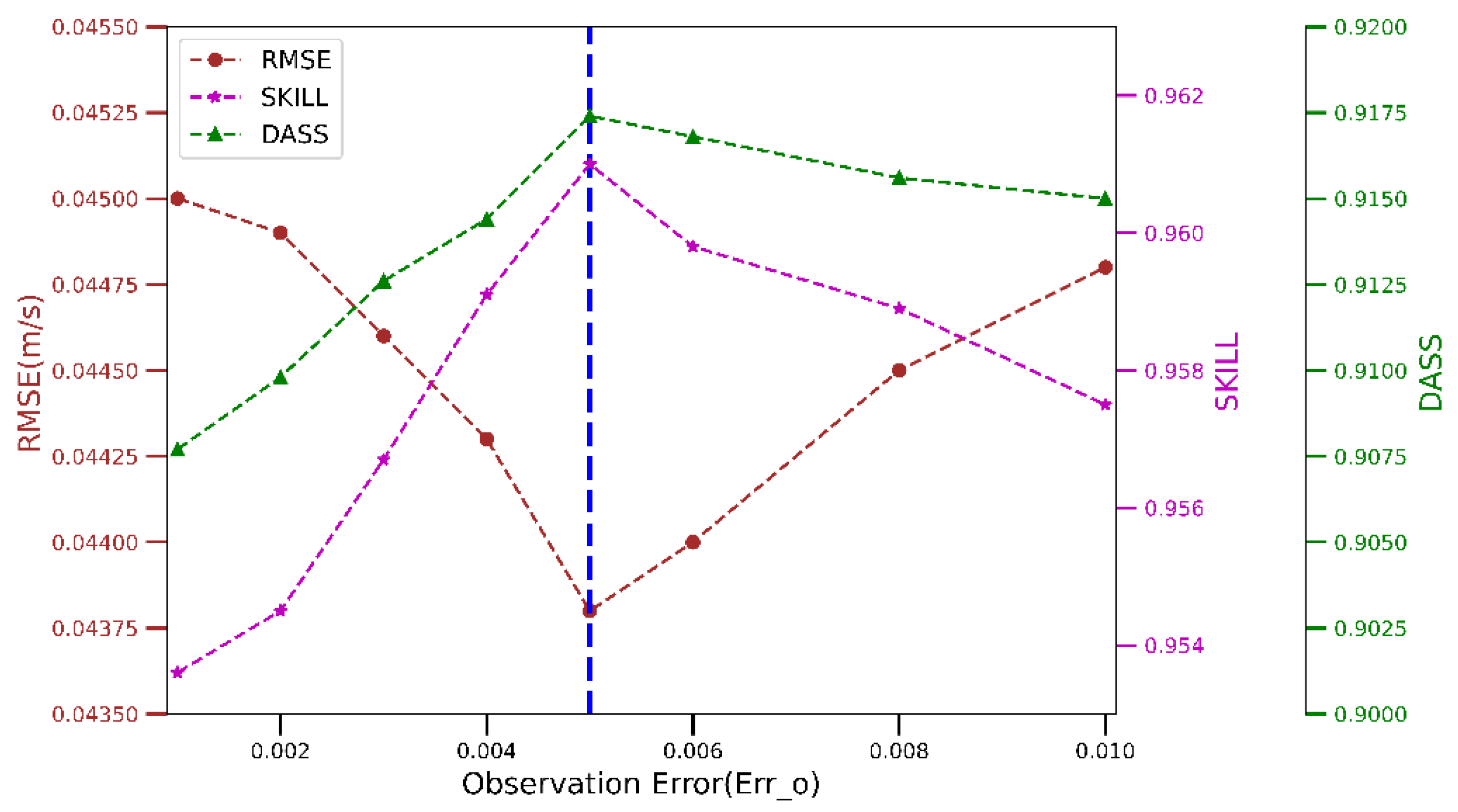
Figure 8 displays the variations in the observation error (Erro) from 0.001 to 0.01 for the model error, and the number of particles was 0.2 and 100, respectively. For the observation errors lower than 0.005, the RMSE showed a steady decline, while SKILL and DASS increased. By increasing the observation error to 0.005, the changes in the three curves followed the opposite trend. Similar to the case of the model error, the three parameters reached their extreme values (0.0438, 0.961, and 0.9174) for an observation error of 0.005.
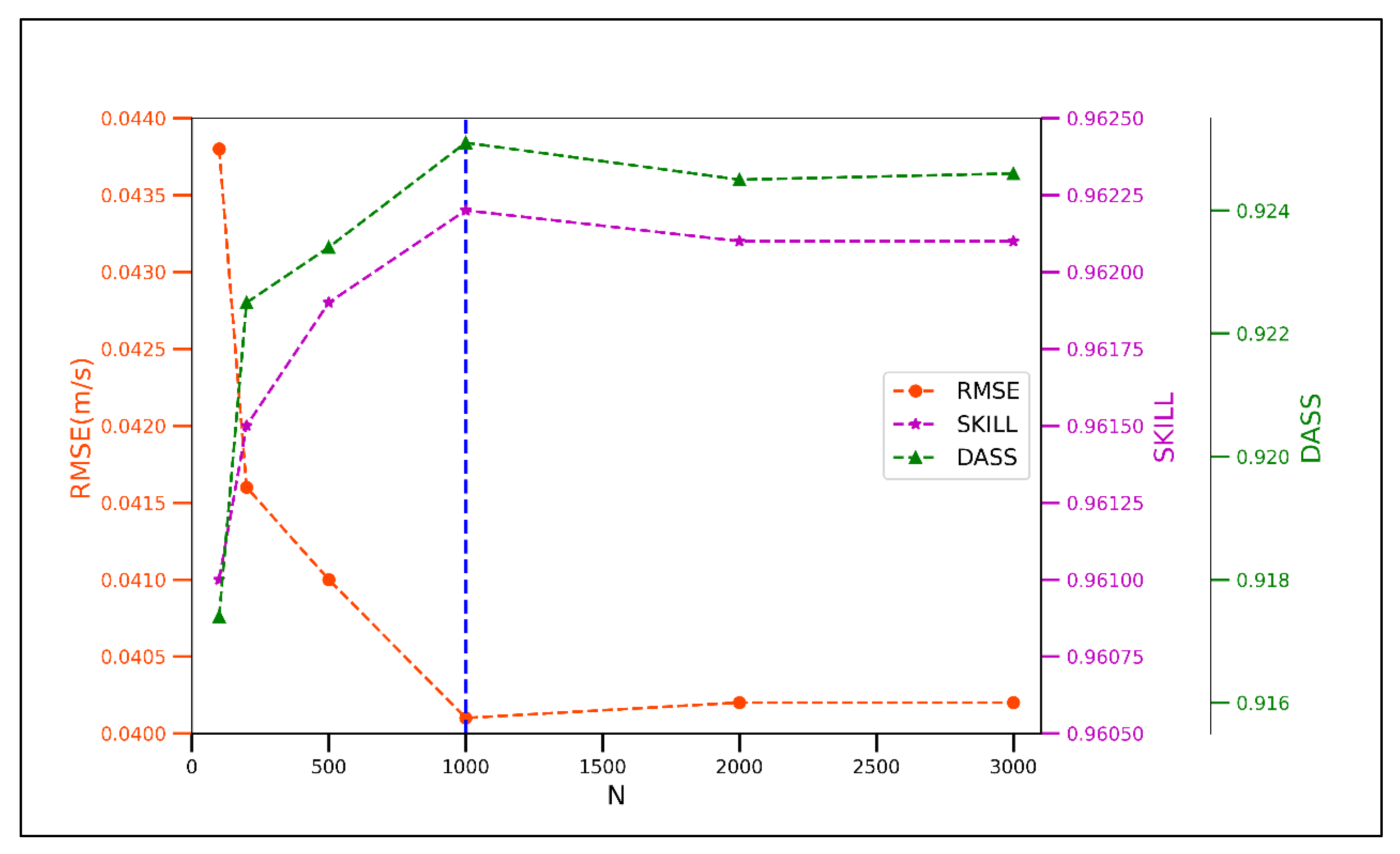
Figure 9 shows the sensitivity of the number of particles (N) in the PF. As expected, by fixing the model error and the observation error values to 0.2 and 0.005, respectively, with the number of particles from 100 to 1000, the RMSE rapidly decreased, while SKILL and DASS steadily increased. The three parameters were 0.0401 m/s, 0.9622, and 0.9251, which were their extreme values for 1000 particles. Beyond that, the RMSE slowly increased, while SKILL and DASS slightly decreased by increasing the number of particles. The final values of the model error, the observation error, and the number of particles were 0.2, 0.005, and 1000, respectively.
3.2. Simulation with Updated Data Assimilation Period
The velocity correction was performed by coupling TELEMAC-3D with the PF in Python through the TELAPY component of the TELEMAC-MASCARET SYSTEM. To evaluate the performance of assimilating the HADCP velocity data, the model settings in the assimilation period were the same as those in the calibration and validation period of the experiment reach. The parameters of the PF, namely the model error, the observation error, and the number of particles, were set to 0.2, 0.05, and 1000, respectively.
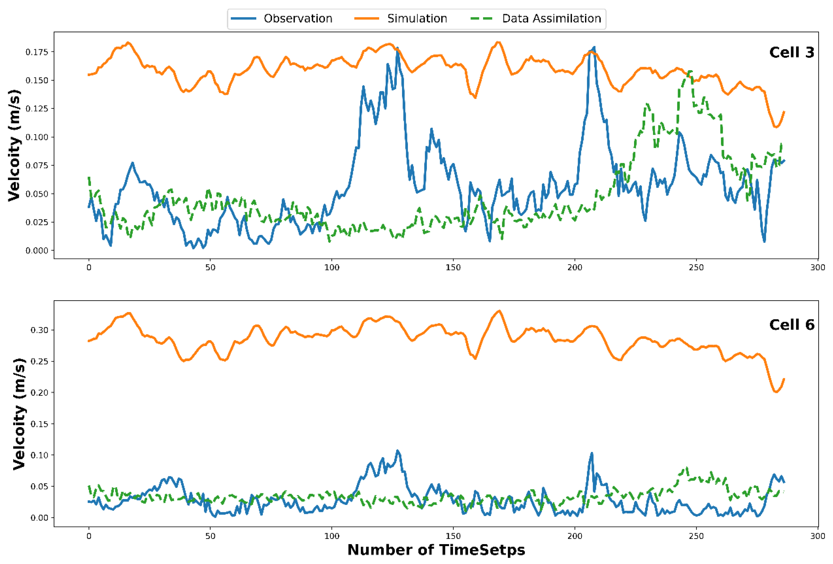
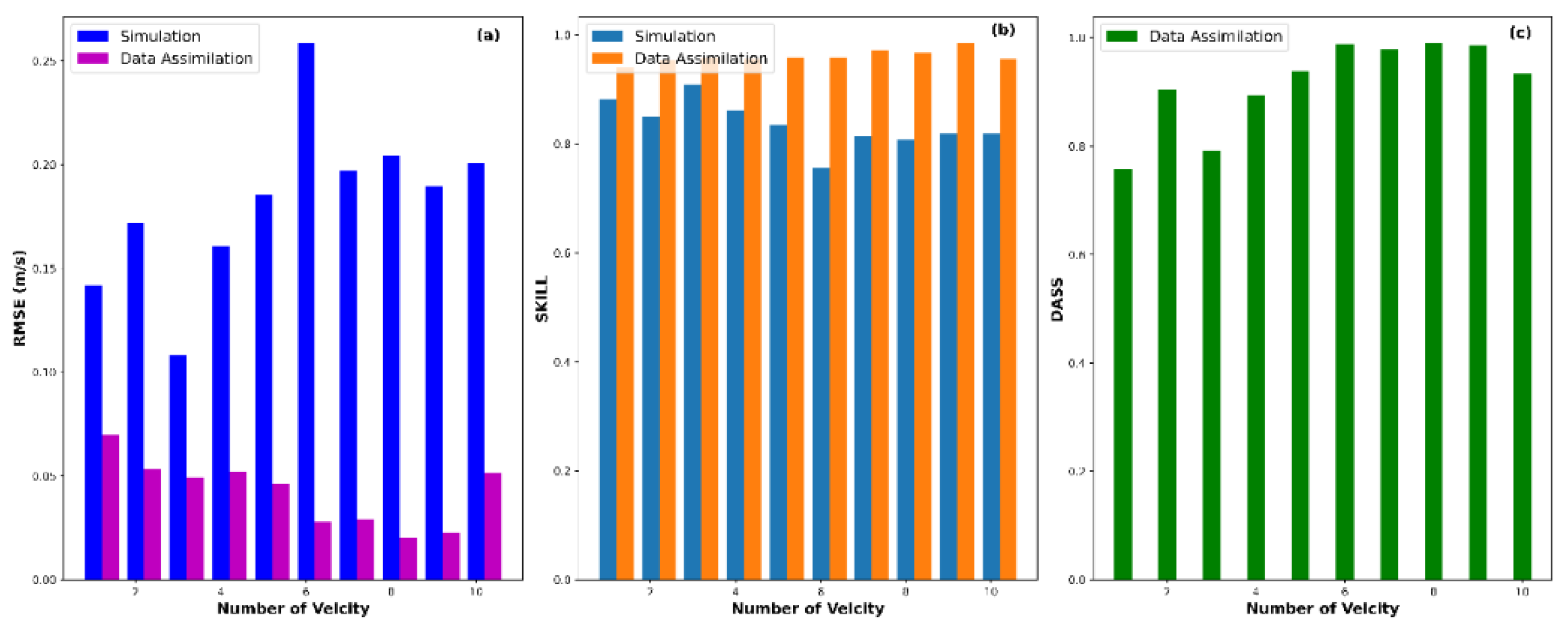
The results of velocity correction on cells 3 and 6 of the HADCP during the assimilation period (7 January 2022) are shown in Figure 10. As expected, the overestimation of velocity significantly improved. The assimilated velocities were also much closer to the observed velocities than the simulated velocities on cells 3 and 6 locations of the HADCP. A similar trend was also seen in other HADCP cell locations. It was also seen that the RMSE significantly declined, whereas SKILL improved, as shown in Figure 11a,b, respectively. Table 4 quantitatively shows the RMSE and SKILL of the 10 cell locations of the HADCP before and after assimilation. After assimilation with the PF, the RMSE of cell 3 decreased from 0.108 m/s to 0.049 m/s with a decrease of 54%, while the SKILL of cell 3 increased by 5.38%, from 0.91 to 0.959. Similarly, when the PF intervened in the model, the RMSE of cell 6 decreased from 0.259 m/s to 0.028 m/s with a decrease of 89.2%, while the SKILL increased by 26.7%, from 0.756 to 0.958. Although the simulation could not capture the peak and trend of the velocity very well after assimilation, as shown in Figure 10, the mean RMSE and SKILL values during the assimilation period (7 January 2022; 24 h) showed significant improvement on each of the 10 cells, as shown in Table 4 and Figure 11a,b; especially notable was the improvement in the RMSE. This shows that all in all, the approach of coupling the 3D hydrodynamic model with DA could correct the simulated velocity. Moreover, the mean RMSE for the 10 cells was reduced to 0.042 m/s from an initial value of 0.182 m/s, showing that the model performance improved with a reduction of 78% the in overall simulation error. Furthermore, SKILL increased from 0.836 to 0.96, indicating that the model’s performance level significantly improved by using the PF. Similarly, DASS was 0.92 (Table 4 and Figure 11c), indicating excellent assimilation performance. Therefore, from the point of view of the improvement in velocity values and model performance, the results of coupling the 3D hydrodynamic model with DA to correct the velocity are encouraging for velocity measurement.
The currently used flow velocity measurement methods have various disadvantages, such as operational complexity, time effectiveness, and accuracy. The approach of using DA to correct the numerical model’s state variables so that the state variables do not deviate from reality is widely used in coastal water and environmental management [11,12,13,14,15] but has not been applied in hydrometry. The results of our practical experiment showed that this approach yielded good results in terms of improving the velocity value and model performance. This implies that coupling 3D hydrodynamic model with DA can improve the accuracy and efficiency of velocity measurement.
Moreover, the experiment presented in this article is an initial attempt to apply the approach of using DA to correct numerical models’ state variables for their use in hydrometry. The future research direction can be to use a variety of observational data (point-wise data, vertical-wise data, and data at a certain level of water body) and data types (water level data, velocity data, roughness factor data, and other data) simultaneously to correct the simulated velocity of the model for improving the accuracy and efficiency of the velocity measurement. Furthermore, this approach can also be applied to measure other hydrological factors in hydrometry, such as water level, sediment, water temperature, and water quality.
4. Conclusions
To improve the accuracy and efficiency of velocity measurements, we proposed a DA scheme coupled with the TELEMAC-3D model and the PF. We used Python scripting using the TELAPY component of the TELEMAC-MASCARET SYSTEM. The validity of the proposed system was demonstrated based on the data collected in a Lanxi River experiment reach. To reproduce the velocity of the reach within reasonable and acceptable ranges, a TELEAMC-3D model for the experiment reach was calibrated and validated. Then, we carried out a sensitivity analysis to identify the PF sensitivity parameters. A modified process was developed to improve the velocity and model performance accuracy by combining the TELEMAC-3D model and the PF. The experimental results indicated that the obtained assimilated velocities were much closer to the observed velocities than the simulated velocities. Although the peak and trend of real velocity were not replicated well, the three statistical measures (RMSE, SKILL, and DASS) were substantially improved on each of the assimilated nodes. Our results showed that the proposed DA scheme coupled with the 3D hydrodynamic model improved the accuracy and efficiency of velocity measurements. In the future, the proposed DA scheme can also be extended to measure other hydrological factors, such as water quality, water temperature, and sediment. The proposed model can be a reasonable alternative to the current velocity measurement techniques and hydrometry techniques.
Author Contributions
Methodology, J.L. (Jiufu Liu); software, Q.C.; validation, L.Z.; writing—original draft, Y.S.; writing—review & editing, J.L. (Jin Lin) All authors have read and agreed to the published version of the manuscript.
Funding
This research received no external funding.
Data Availability Statement
Data sharing not applicable.
Conflicts of Interest
The authors declare no conflict of interest.
References
- Turnipseed, D.P.; Sauer, V.B. Discharge Measurements at Gaging Stations; Techniques and Methods 3-A8; U.S. Geological Survey: Reston, VA, USA, 2010; p. 87. [CrossRef]
- Dobriyal, P.; Badola, R.; Tuboi, C.; Hussain, S.A. A review of methods for monitoring streamflow for sustainable water resource management. Appl. Water Sci. 2016, 7, 2617–2628. [Google Scholar] [CrossRef] [Green Version]
- Boman, B.; Shukla, S. Water Measurement for Agricultural Irrigation and Drainage Systems; Agricultural and Biological Engineering Department, Florida Cooperative Extension Service, University of Florida: Gainesville, FL, USA, 2009. [Google Scholar]
- Chauhan, M.S.; Kumar, V.; Dikshit, P.K.S.; Dwivedi, S.B. Comparison of discharge data using ADCP and current meter. Int. J. Adv. Earth Sci. 2014, 3, 81–86. [Google Scholar]
- Boldt, J.A.; Oberg, K.A. Validation of streamflow measurements made with M9 and River Ray acoustic Doppler current profilers. J. Hydraul. Eng. 2015, 142, 04015054. [Google Scholar] [CrossRef] [Green Version]
- Fulton, J.W. Guidelines for Siting and Operating Surface-Water Velocity Radars; Technical report; USGS: Reston, VA, USA, 2020.
- Creutin, J.D.; Muste, M.; Bradley, A.A.; Kim, S.C.; Kruger, A. River gauging using PIV techniques: A proof of concept experiment in the Iowa River. J. Hydrol. 2003, 277, 182–194. [Google Scholar] [CrossRef]
- Neal, J.; Schumann, G.; Bates, P.; Buytaert, W.; Matgen, P.; Pappenberger, F. A data assimilation approach to discharge estimation from space. Hydrol. Process. 2009, 23, 3641–3649. [Google Scholar] [CrossRef]
- Qi, L.; Ma, R.; Hu, W.; Loiselle, S.A. Assimilation of MODIS chlorophyll-a data into a coupled hydrodynamic-biological model of Taihu Lake. IEEE J. Sel. Top. Appl. Earth Obs. Remote Sens. 2014, 7, 1623–1631. [Google Scholar] [CrossRef]
- Bannister, R. A review of operational methods of variational and ensemble-variational data assimilation. Q. J. R. Meteorol. Soc. 2017, 143, 607–633. [Google Scholar] [CrossRef] [Green Version]
- Akiko, M.; Olli, M.; Sampsa, K.; Kari, K.; Antti, T.; Janne, R.; Janne, J.; Ninni, L. Assimilation of satellite data to 3D hydrodynamic model of Lake Säkylän Pyhäjärvi. Water Sci. Technol. 2015, 71, 1033–1039. [Google Scholar] [CrossRef]
- Nowicki, A.; Janecki, M.; Darecki, M.; Piotrowski, P.; Dzierzbicka-Głowacka, L. The Use of Satellite Data in the Operational 3D Coupled Ecosystem Model of the Baltic Sea (3D Cembs). Pol. Marit. Res. 2016, 23, 20–24. [Google Scholar] [CrossRef] [Green Version]
- Wang, X.; Zhang, J.; Babovic, V.; Gin, K.Y.H. A Comprehensive Integrated Catchment-Scale Monitoring and Modelling Approach for Facilitating Management of Water Quality. Environ. Model. Softw. 2019, 120, 104489. [Google Scholar] [CrossRef]
- Baracchini, T.; Chu, P.Y.; Šukys, J.; Lieberherr, G.; Wunderle, S.; Wüest, A.; Bouffard, D. Data assimilation of in situ and satellite remote sensing data to 3D hydrodynamic lake models: A case study using Delft3D-FLOW v4.03 and OpenDA v2.4. Geosci. Model Dev. 2020, 13, 1267–1284. [Google Scholar] [CrossRef] [Green Version]
- Janecki, M.; Dybowski, D.; Jakacki, J.; Nowicki, A.; Dzierzbicka-Glowacka, L. The Use of Satellite Data to Determine the Changes of Hydrodynamic Parameters in the Gulf of Gdańsk via EcoFish Model. Remote Sens. 2021, 13, 3572. [Google Scholar] [CrossRef]
- Barthélémya, S.; Riccia, S.; Morela, T.; Goutalb, N.; le Papec, E.; Zaoui, F. On operational flood forecasting system involving 1D/2D coupled hydraulic model and data assimilation. J. Hydrol. 2018, 562, 623–634. [Google Scholar] [CrossRef]
- García-Pintado, J.; Mason, D.C.; Dance, S.L.; Cloke, H.L.; Neal, J.C.; Freer, J.; Bates, P.D. Satellite-supported flood forecasting in river networks: A real case study. J. Hydrol. 2015, 523, 706–724. [Google Scholar] [CrossRef] [Green Version]
- Barthélémy, S.; Ricci, S.; Rochoux, M.C.; Le Pape, E.; Thual, O. Ensemble-based data assimilation for operational flood forecasting—On the merits of state estimation for 1D hydrodynamic forecasting through the example of the ‘‘Adour Maritime” river. J. Hydrol. 2017, 552, 210–224. [Google Scholar] [CrossRef]
- Costi, J.; Marques, W.; Kirinus, E.; Duarte, R.; Arigony-Neto, J. Water level variability of the Mirim-São Gonçalo, a large subtropical semi-enclosed coastal system. Adv. Water Resour. 2018, 117, 75–86. [Google Scholar] [CrossRef]
- Maerker, C.; Malcherek, A.; Riemann, J.; Brudy-Zippelius, T. Modelling and analysing dredging and disposing activities by use of Telemac, Sisyphe and DredgeSim. In Proceedings of the Telemac User Conference, Paris, France, 19–21 October 2011; pp. 92–98. [Google Scholar]
- da Silva, M.C.; Kirinus, E.D.P.; Bendô, A.R.R.; Marques, W.C.; Vargas, M.M.; Leite, L.R.; Junior, O.O.M.; Pertille, J. Dynamic modeling of effluent dispersion on Mangueira bay–Patos Lagoon (Brazil). Reg. Stud. Mar. Sci. 2020, 41, 101544. [Google Scholar] [CrossRef]
- Kirinus, E.D.P.; Oleinik, P.H.; Costi, J.; Marques, W.C. Long-term simulations for ocean energy off the Brazilian coast. Energy 2018, 163, 364–382. [Google Scholar] [CrossRef]
- Corti, S.; Pennati, V. A 3-D hydrodynamic model of river flow in a delta region. Hydrol. Process. 2000, 14, 2301–2309. [Google Scholar] [CrossRef]
- Bitencourt, L.P.; Fernandes, E.H.; da Silva, P.D.; Möller, O., Jr. Spatio-temporal variability of suspended sediment concentrations in a shallow and turbid lagoon. J. Mar. Syst. 2020, 212, 103454. [Google Scholar] [CrossRef]
- Fernandes, E.H.; da Silva, P.D.; Gonçalves, G.A.; Möller, O.O., Jr. Dispersion Plumes in Open Ocean Disposal Sites of Dredged Sediment. Water 2021, 13, 808. [Google Scholar] [CrossRef]
- Hervouet, J.M. Hydrodynamics of Free Surface Flows: Modeling with the Finite Element Method; Wiley: Hoboken, NJ, USA, 2007. [Google Scholar]
- Telemac-3d: Theory Guide; Tech. Rep.; EDF: Paris, France, 2019.
- TelApy: User manual; Tech. Rep.; EDF: Paris, France, 2019.
- Goeury, C.; Audouin, Y.; Zaoui, F. Interoperability and computational framework for simulating open channel hydraulics: Application to sensitivity analysis and calibration of Gironde Estuary model. Environ. Model. Softw. 2022, 148, 105243. [Google Scholar] [CrossRef]
- Moradkhani, H.; Hsu, K.; Gupta, H.; Sorooshian, S. Uncertainty assessment of hydrologic model states and parameters: Sequential data assimilation using the particle filter. Water Resour. Res. 2005, 41, W05012. [Google Scholar] [CrossRef] [Green Version]
- Liu, J.S.; Chen, R. Sequential monte carlo methods for dynamic systems. J. Am. Stat. Assoc. 1998, 93, 1032–1044. [Google Scholar] [CrossRef]
- Gordon, N.J.; Salmond, D.J.; Smith, A.F.M. Novel approach to nonlinear/non-Gaussian Bayesian state estimation. IEEE Proc. F Radar Signal Process. 1993, 140, 107–113. [Google Scholar] [CrossRef] [Green Version]
- Telemac-3d: User Manual; Tech. Rep.; EDF: Paris, France, 2019.
- Maréchal, D. A Soil-based Approach to Rainfall-Runoff Modeling in Ungauged Catchments for England and Wales; Cranfield University: Cranfield, UK, 2004. [Google Scholar]
- Ren, L.; Hartnett, M. Hindcasting and Forecasting of Surface Flow Fields through Assimilating High Frequency Remotely Sensing Radar Data. Remote Sens. 2017, 9, 932. [Google Scholar] [CrossRef] [Green Version]
- Ren, L.; Nash, S.; Hartnett, M. Forecasting of Surface Currents via Correcting Wind Stress with Assimilation of High-Frequency Radar Data in a Three-Dimensional Model. Adv. Meteorol. 2016, 2016, 8950378. [Google Scholar] [CrossRef] [Green Version]
- Wan, Y.; Ji, Z.-G.; Shen, J.; Hu, G.; Sun, D. Three-dimensional water quality modeling of a shallow subtropical estuary. Mar. Environ. Res. 2012, 82, 76–86. [Google Scholar] [CrossRef]
Figure 1.
A 3D mesh of TELEMAC-3D model built from a 2D mesh.

Figure 2.
Overview of the TELAPY module [29].
Figure 2.
Overview of the TELAPY module [29].

Figure 3.
(a) Map of Lanxi River; (b) a 2D computation mesh of the considered experiment reach; (c) the 10 cell locations of HADCP and mesh size of the considered experiment reach; (d) details of the 10 cell locations of HADCP.
Figure 3.
(a) Map of Lanxi River; (b) a 2D computation mesh of the considered experiment reach; (c) the 10 cell locations of HADCP and mesh size of the considered experiment reach; (d) details of the 10 cell locations of HADCP.

Figure 4.
The flowchart of the proposed DA scheme for soft velocity measurement coupled with the TELEMAC-3D model and PF.
Figure 4.
The flowchart of the proposed DA scheme for soft velocity measurement coupled with the TELEMAC-3D model and PF.

Figure 5.
The calibration exercise compares the simulated (orange line) and observed (blue line) flow velocity from 06:00 to 23:59 on 5 January 2022.
Figure 5.
The calibration exercise compares the simulated (orange line) and observed (blue line) flow velocity from 06:00 to 23:59 on 5 January 2022.

Figure 6.
The validation exercise compares the simulated (orange line) and observed (blue line) flow velocity on 6 January 2022.
Figure 6.
The validation exercise compares the simulated (orange line) and observed (blue line) flow velocity on 6 January 2022.

Figure 7.
Model error (Errm) versus RMSE, SKILL, and DASS of PF.

Figure 8.
Observation error (Erro) versus RMSE, SKILL, and DASS of PF.

Figure 9.
RMSE, SKILL, and DASS of PF versus the number of particles, N.

Figure 10.
Comparison of the simulated (orange solid line), observed (blue solid line), and assimilated (green dotted line) flow velocity during assimilating period.
Figure 10.
Comparison of the simulated (orange solid line), observed (blue solid line), and assimilated (green dotted line) flow velocity during assimilating period.

Figure 11.
(a) Comparison of RMSE for the simulation and DA; (b) comparison of SKILL of the simulation and DA; (c) DASS of the experiment during the assimilation period.
Figure 11.
(a) Comparison of RMSE for the simulation and DA; (b) comparison of SKILL of the simulation and DA; (c) DASS of the experiment during the assimilation period.


Table 1.
Velocity estimation methods and their characteristics [2].
Table 1.
Velocity estimation methods and their characteristics [2].
| Method | Operational Complexity | Cost-Effectiveness | Accuracy | Time-Effectiveness | Ecological Impact |
|---|---|---|---|---|---|
| Float method | Easy | Inexpensive | Low | Efficient | Non-polluting |
| Dilution gauging method | Difficult | Inexpensive | Low | Efficient | Affects the stream ecosystem |
| Trajectory method | Difficult | Inexpensive | High | Inefficient | Non-polluting |
| Current meter method | Difficult | Expensive | High | Efficient | Non-polluting |
| Acoustic Doppler’s current profiler method | Difficult | Expensive | High | Efficient | Non-polluting |
| Electromagnetic method | Difficult | Expensive | High | Efficient | Non-polluting |
| Remote sensing method | Difficult | Expensive | Low | Efficient | Non-polluting |
| Particle image velocimetry | Difficult | Expensive | High | Efficient | Non-polluting |
Table 2.
The RMSE and SKILL values of the calibration and validation exercises of the TELEMAC-3D model.
Table 2.
The RMSE and SKILL values of the calibration and validation exercises of the TELEMAC-3D model.
| Trial | Verification Metrics | Number of Cell | ||||||||||
|---|---|---|---|---|---|---|---|---|---|---|---|---|
| 1 | 2 | 3 | 4 | 5 | 6 | 7 | 8 | 9 | 10 | Mean | ||
| Calibration Exercise | RMSE | 0.114 | 0.147 | 0.088 | 0.134 | 0.161 | 0.237 | 0.176 | 0.183 | 0.183 | 0.178 | 0.16 |
| SKILL | 0.915 | 0.884 | 0.934 | 0.894 | 0.865 | 0.779 | 0.84 | 0.831 | 0.824 | 0.85 | 0.86 | |
| Validation Exercise | RMSE | 0.142 | 0.171 | 0.103 | 0.156 | 0.179 | 0.248 | 0.192 | 0.19 | 0.177 | 0.199 | 0.175 |
| SKILL | 0.879 | 0.849 | 0.913 | 0.863 | 0.839 | 0.768 | 0.819 | 0.824 | 0.83 | 0.821 | 0.84 | |
Table 3.
The sensitivity parameter settings of the particle filter.
| Trial | Parameters | Verification Metrics | ||||
|---|---|---|---|---|---|---|
| Model Error (m/s) | Observation Error (m/s) | Number of Particles (-) | RMSE (m/s) | SKILL (-) | DASS (-) | |
| 1 | 0.01 | 0.001 | 100 | 0.1862 | 0.9055 | −0.0505 |
| 2 | 0.05 | - | - | 0.1542 | 0.9141 | 0.3023 |
| 3 | 0.08 | - | - | 0.091 | 0.9326 | 0.7523 |
| 4 | 0.1 | - | - | 0.0533 | 0.9471 | 0.8974 |
| 5 | 0.2 | - | - | 0.045 | 0.9536 | 0.9077 |
| 6 | 0.2 | 0.002 | 0.0449 | 0.9545 | 0.9098 | |
| 7 | 0.2 | 0.003 | 0.0446 | 0.9567 | 0.9126 | |
| 8 | 0.2 | 0.004 | 0.0443 | 0.9591 | 0.9144 | |
| 9 | 0.2 | 0.005 | - | 0.0438 | 0.961 | 0.9174 |
| 10 | 0.2 | 0.005 | 200 | 0.0416 | 0.9615 | 0.9225 |
| 11 | 0.2 | 0.005 | 500 | 0.041 | 0.9619 | 0.9234 |
| 12 | 0.2 | 0.005 | 1000 | 0.0401 | 0.9622 | 0.9251 |
Table 4.
RMSE, SKILL, and DASS of the simulations and DA in the assimilation time.
| Trial | Verification Metrics | Number of Cell | ||||||||||
|---|---|---|---|---|---|---|---|---|---|---|---|---|
| 1 | 2 | 3 | 4 | 5 | 6 | 7 | 8 | 9 | 10 | Mean | ||
| SIM | RMSE | 0.142 | 0.172 | 0.108 | 0.16 | 0.186 | 0.259 | 0.197 | 0.204 | 0.19 | 0.201 | 0.182 |
| SKILL | 0.882 | 0.849 | 0.91 | 0.861 | 0.836 | 0.756 | 0.815 | 0.808 | 0.819 | 0.819 | 0.836 | |
| DA | RMSE | 0.07 | 0.053 | 0.049 | 0.052 | 0.046 | 0.028 | 0.029 | 0.021 | 0.022 | 0.051 | 0.042 |
| SKILL | 0.94 | 0.954 | 0.959 | 0.956 | 0.958 | 0.958 | 0.971 | 0.968 | 0.985 | 0.957 | 0.96 | |
| DASS | 0.759 | 0.904 | 0.791 | 0.894 | 0.939 | 0.989 | 0.978 | 0.99 | 0.986 | 0.934 | 0.92 | |
Publisher’s Note: MDPI stays neutral with regard to jurisdictional claims in published maps and institutional affiliations. |
© 2022 by the authors. Licensee MDPI, Basel, Switzerland. This article is an open access article distributed under the terms and conditions of the Creative Commons Attribution (CC BY) license (https://creativecommons.org/licenses/by/4.0/).
Share and Cite
MDPI and ACS Style
Sun, Y.; Zhang, L.; Liu, J.; Lin, J.; Cui, Q. A Data Assimilation Approach to the Modeling of 3D Hydrodynamic Flow Velocity in River Reaches. Water 2022, 14, 3598. https://doi.org/10.3390/w14223598
AMA Style
Sun Y, Zhang L, Liu J, Lin J, Cui Q. A Data Assimilation Approach to the Modeling of 3D Hydrodynamic Flow Velocity in River Reaches. Water. 2022; 14(22):3598. https://doi.org/10.3390/w14223598
Chicago/Turabian StyleSun, Yixiang, Lu Zhang, Jiufu Liu, Jin Lin, and Qingfeng Cui. 2022. "A Data Assimilation Approach to the Modeling of 3D Hydrodynamic Flow Velocity in River Reaches" Water 14, no. 22: 3598. https://doi.org/10.3390/w14223598
Note that from the first issue of 2016, this journal uses article numbers instead of page numbers. See further details here.