
Covariance-Based Selection of Parameters for Particle Filter Data Assimilation in Soil Hydrology
Faculty of Civil and Environmental Engineering, Technion-Israel Institute of Technology, Derech Ya’akov Dori, Haifa 3200003, Israel
*
Author to whom correspondence should be addressed.
Water 2022, 14(22), 3606; https://doi.org/10.3390/w14223606
Submission received: 4 October 2022
/
Revised: 6 November 2022
/
Accepted: 7 November 2022
/
Published: 9 November 2022
(This article belongs to the Section Soil and Water)
Abstract
:Real-time in situ measurements are increasingly being used to improve the estimations of simulation models via data assimilation techniques such as particle filter. However, models that describe complex processes such as water flow contain a large number of parameters while the data available are typically very limited. In such situations, applying particle filter to a large, fixed set of parameters chosen a priori can lead to unstable behavior, i.e., inconsistent adjustment of some of the parameters that have only limited impact on the states that are being measured. To prevent this, in this study correlation-based variable selection is embedded in the particle filter, so that at each step only a subset of the most influential parameters is adjusted. The particle filter used in this study includes genetic algorithm operators and Monte Carlo Markov Chain for alleviating filter degeneracy and sample impoverishment. The proposed method was applied to a water flow model (Hydrus-1D) in which soil water content at various depths and soil hydraulic parameters were updated. Two case studies are presented. Overall, the proposed method yielded parameters and states estimates that were more accurate and more consistent than those obtained when adjusting all the parameters. Furthermore, the results show that the higher the influence of a parameter on the model output under the current conditions, the better the estimation of this parameter is.
1. Introduction
Accurate and proper estimation of prognostic variables (e.g., soil moisture) has been receiving increasing attention in the past years. The mathematical models that describe such complex processes (e.g., Hydrus [1]) contain a large number of parameters. Calibrating such models, which are non-linear, is far from trivial, especially since in real settings the data available for the task are limited. Therefore, real-time in situ measurements are increasingly being used to improve the estimations of such simulation models via data assimilation techniques [2,3,4,5,6,7,8].
One of the most widely used data assimilation (DA) methods is the ensemble Kalman filter (EnKF) [8,9,10]. Despite the popularity of EnKF, this technique requires determining some factors, such as covariance inflation and covariance localization, which strongly influence the behavior of the EnKF. To overcome these limitations, particle filter (PF) has been increasingly used as an alternative data assimilation method [11,12,13].
A main drawback of PF is particle degeneracy as some particles become associated with negligible weights. Several methods have been suggested to mitigate this problem. Moradkhani et al. [14], who worked with a hydrological model, suggested perturbing the parameters using Gaussian noise. Another method suggested to handle weight degeneracy is the combination of PF with Monte Carlo Markov Chain (MCMC) [15,16]. This integration helps the PF to replace low probability particles with particles that have higher probabilities. On the other hand, intelligent search and optimization methods, such as Genetic algorithm (GA), have been used as well to alleviate the degeneracy problem. Jamal and Linker [13] showed the usefulness combining MCMC and PF with Genetic operators of GA (named GPFM). This approach was applied to simultaneous estimation of state variables and parameters in a crop growth model.
As mentioned above, the models that describe complex processes such as water flow and/or crop development (e.g., Soil Water Atmosphere Plant (SWAP) model [17]) contain a large number of parameters and the data available are rarely sufficient for calibrating all the parameters at once. In such cases, a sub-set of the most influential parameters should be calibrated rather than attempting to calibrate all the parameters at once. This process of parameter selection can be performed beforehand via sensitivity analysis [18,19,20,21]. However, the results of the sensitivity analysis can be somehow misleading or irrelevant since the “importance” of a specific parameter depends on the state of the system. For instance, in soil hydrology, the residual water content has a strong influence on the model behavior during dry periods while its value is basically irrelevant during wet periods. Similarly, hydraulic conductivity can be more influential during wet periods than during dry ones [22]. Therefore, the calibration of the residual water content during wet periods is at best unnecessary and can even cause a degradation of the estimated value [13]. Therefore, when data assimilation (rather than off-line batch calibration) is considered, the sensitivity of the parameters should be determined dynamically in real-time.
A number of studies have considered the concept of real-time sensitivity analysis for model calibration. In [23], the running period was split into sub-periods and the corresponding influential parameters were calibrated. In [24], integrating real-time sensitivity with data assimilation in irrigation scheduling was shown to result in an improvement in profit. In [25], particle filter was linked to a sensitivity analysis for improving the accuracy of AquaCrop, and the results showed superior estimations in comparison to the conventional particle filter. Furthermore, it was found that capturing the varying parameters sensitivity requires real-time sensitivity analysis.
While performing “true” sensitivity analysis in real-time is accompanied with high computational burden, an alternative is to use correlation analysis [26] for quantifying the sensitivity of the parameters. Many authors refer to a parameter as ‘sensitive’, ‘most influential‘, or ‘correlate’, when a model result can be highly correlated with an input parameter so that small changes in the parameter value results in significant changes in the outputs [18]. The concept of correlation analysis is to evaluate the correlation between the updated variables and the measured ones, which in turn can be used to identify the most influential parameters. The usage of correlation analysis for parameter selection in data assimilation is limited. However, correlation analysis is used somehow in Kalman filters through the Kalman gain calculation. Hu et al. [27], who reported data assimilation in a crop model, suggested using states correlations, in addition to the traditional use of correlation analysis for determining the Kalman gain, in order to prevent updating poorly correlated states. State variables with low correlation to the measurements (or measured states) are updated less frequently than the highly correlated ones.
In traditional particle filters, the whole set of parameters is updated, regardless of the sensitivity or correlation of each parameter inside this set to the available measurements [7,15]. This study presents a novel particle filter in which correlation-based variable selection is embedded. Whenever measurements become available, the most influential (i.e., the most highly correlated) parameters are determined by correlation analysis, and only these parameters are updated by PF. More specifically, the data assimilation technique of genetic-operator-based PF with Monte Carlo Markov Chain (based on [13]) is combined with calculation of the correlation between each parameter and each measured state. Then, only highly correlated parameters are involved in the selection, mutation, crossover and resampling operations of the PF, leading to the novel approach denoted C-GPFM. The proposed method is applied to a water flow model (Hydrus-1D) in which states (soil water contents) and parameters (soil hydraulic parameters) are updated via data assimilation. Hydrus-1D numerically solves the Richards equation for saturated–unsaturated water flow and Fickian-based advection dispersion equations for heat and solute transport. The model parameters are the soil hydraulic parameters of van Genuchten-Mualem equation [1]. Two case studies were generated and analyzed in order to investigate the performance of the proposed method. The results of the proposed method are compared to the case where the whole set of parameters is updated.
2. Methods
2.1. Particle Filtering
Nonlinear dynamic systems are often described by the following finite difference equations [28]:
where ( ) denotes the model, denotes the measurements operator, denotes the state vector at time , is the (uncertain) forcing input, is the vector of model parameters, is the vector of measured variables. and are the process and measurements noise, respectively, which are assumed to be white noises with zero mean and covariance and , respectively. In addition, they are assumed to be independent. Based on Bayesian estimation, given a measurement at time the posterior distribution of the state at time is as follows [29]:
where is the likelihood of the observed measurement given the estimated state at time , is the prior distribution of the state, and is a normalization factor. The marginal likelihood function can be computed as:
The analytical solution of (3) cannot be obtained due to the non-linearity of the process and the multi-dimensionality of the problem. In procedures based on particle filter, the posterior distribution is approximated using an ensemble of particles, that is by running an ensemble of models in parallel. Whenever a measurement becomes available, the state probability for each particle is estimated using (3). Each particle consists of a state and parameter set. Based on the probabilities, the weight associated with each particle is calculated. The higher the weight, the higher the probability that the particle is representing the posterior and the higher the importance of the particle [13]. The reader is referred to [14] for a more detailed description of particle filters.
The specific PF procedure implemented in this work was the genetic operator-based particle filter combined with Markov Chain Monte Carlo (GPFM), described in [13]. This procedure integrates GA operators and MCMC within the PF. The integration of GA operators with particle filter enables the generation of new offspring models from a high-weight models. The MCMC was used for dropping low-weight models and keeping high-weight models. By these methods, the so-called sample impoverishment and filter degeneracy are alleviated [13]. Notice that the final resampling operation, which was defined as optional in [13], was implemented in the present study via stochastic universal resampling [30].
2.2. Correlation Analysis
As mentioned in the Introduction, the main novelty in this work is the combination of correlation analysis with the particle filter, in-real time. The purpose is to involve only a subset of the parameters in the crossover and mutation operations, in the MCMC and in the resampling process steps of the GPFM procedure.
In order to determine the parameters most highly correlated with the available measurements, the correlation coefficient [31] between each parameter and each measured state is calculated using the particle set while running the particle filter, as follows:
where denotes the -th parameter in particle at time , denotes the -th predicted measured state in particle at time and is the ensemble size. and are the standard deviations of the -th parameter and -th predicted output at time which are calculated as follows:
The correlation coefficient ranges from 0 to 1, corresponding to weak and strong correlation, respectively. A value of 0 means that there is no linear relation between the variables, while 1 means that there is a fully linear relation between the variables. A linear relation between a parameter and a state indicates that when the parameter changes, the state changes accordingly. In this case, the parameter is highly sensitive [32]. After the calculation of the correlation coefficients, the weighted average of the correlation coefficients for each parameter is calculated in order to take into account the correlation of the parameter with all of the measurements. These weights are dictated by the importance of the measurements (or measured states) in the particles weights, i.e., the larger the value of the weight of the measurement in the particle weights, the larger its weight in the correlation coefficient. Therefore, the weight of each measured state correlation coefficient was chosen according to the importance of the measurement in the particles’ weights calculation. The weighted average of the correlation coefficient for each parameter is calculated as follows:
where is the correlation coefficient of parameter at time and denotes the likelihood function. is the importance of measurement on time step , which is calculated based its relative contribution to the particle weight, as follows:
where is the likelihood of measurement given the state and parameter of particle . Noteworthy, is between 0 and 1. It is worth mentioning that the correlation coefficients are calculated based on the prior ensemble (i.e., the particles before performing the crossover and mutation operations) since the proposal parameters are directly influenced by crossover and mutation while the prior ensemble is more physically driven. Physically driven particles (prior) have the real correlation, but operator-driven particles (posterior) include the randomness of the operators [13].
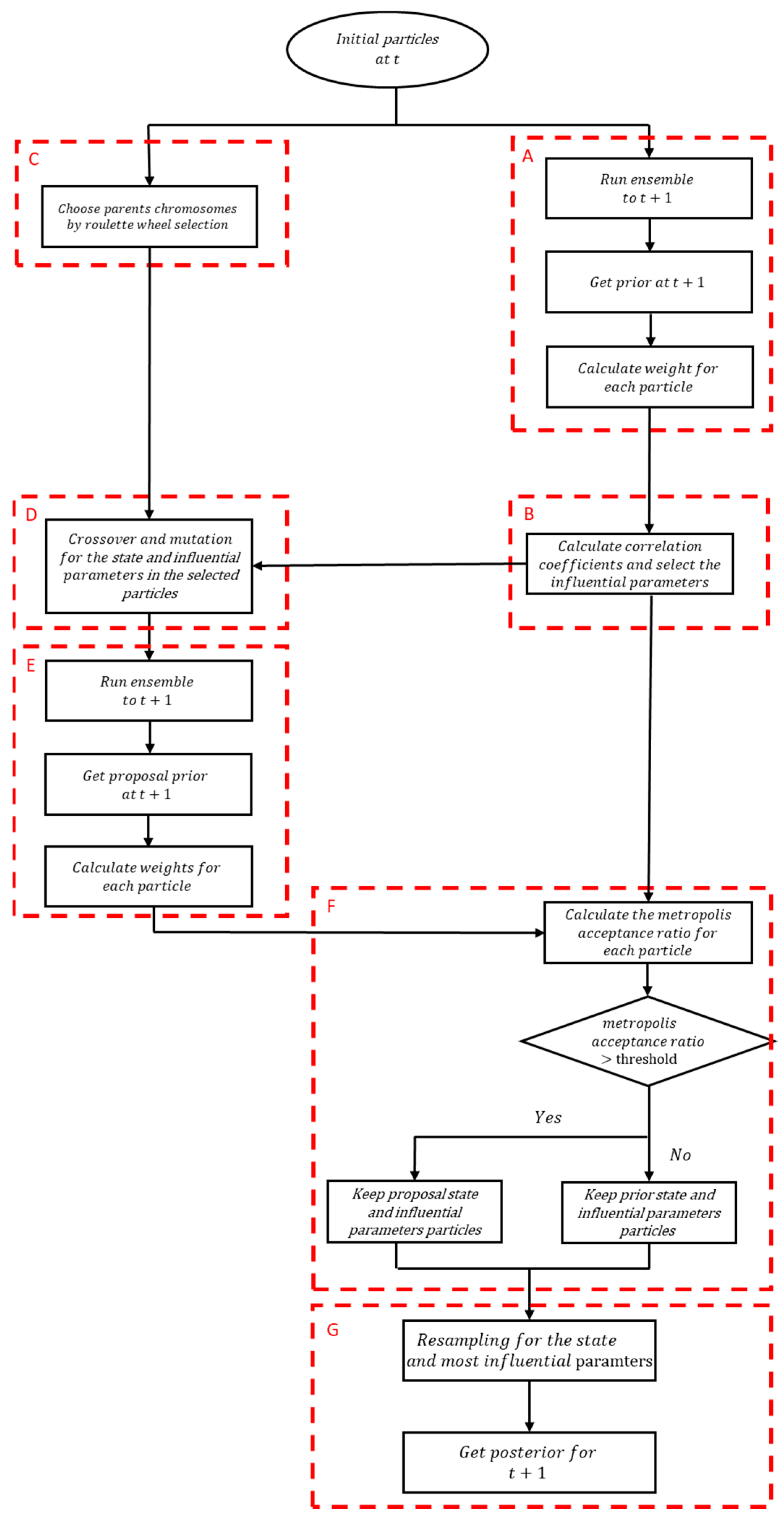
After the calculation of for each parameter, the parameters are ranked from highly influential to low importance based on their correlation coefficients and only the parameters with correlation coefficients above a given threshold are chosen for crossover, mutation, MCMC and resampling. Figure 1 describes the overall framework. The first step (Step A) is to perform one-step-ahead predictions with the whole ensemble and compute the weight associated with each particle. The second step is to calculate the correlation coefficients and select the most influential parameters (Step B). The third step (Step C) is to select particles by roulette wheel selection. Crossover and mutation are then applied on the most influential parameters from Step B (Step D). One-step predictions are performed with the new ensemble (Step E) and the results of each pair of prior/proposal particles are compared to determine which particle must be retained (Step F). Finally, resampling is applied (Step G) over the state and most influential parameters to generate the new particles.
3. Case Studies
The method described above was tested with a synthetic case study of a 1D soil profile with three layers. Two models were created, denoted ‘true’ and ‘biased’. Simulations with the ‘true’ model were performed to generate synthetic measurements and the data assimilation procedure was applied to a model which was initialized as the ‘biased’ model. The estimations of the parameters were restricted to an interval of ±40% around the values of the parameters of the ‘biased’ model. The soil hydraulic properties of the two models are described in Table 1. The parameter values were such that the flow is highly dynamic (sand to loamy sand, using the Rosetta tool from Hydrus-1D [33]) and therefore the problem is challenging. The lower bound condition was set to free drainage, and the initial conditions were set as 0.35 and 0.20 soil water content for the whole profile for the ’true’ and ’biased’ models, respectively. Soil water content at 18 cm and 42 cm were ‘measured’ daily with white Gaussian noise with a standard deviation of 1%.
The ensemble size was chosen as 100. The crossover factor for state and parameters were set to 0.01 and 0.05, respectively. For the mutation for the state and parameters, 10% standard deviation was chosen. Larger crossover was set for the parameters than for the state in order to favor improvement of the model’s dynamics over mere instantaneous adjustment of the state. The threshold of correlation in Equation (8) was set arbitrarily to 0.2, which corresponds to a non-negligible linear relationship [34].
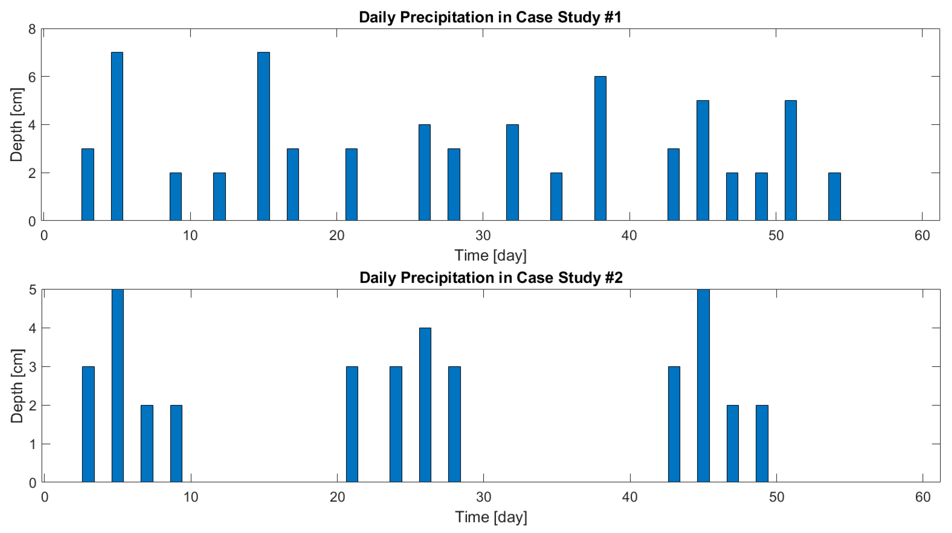
A first study was conducted with random precipitation as a boundary condition, which mimics a typical rainy period. A second analysis was carried out with boundary conditions consisting of ten days irrigation–drainage cycles. This analysis was conducted to evaluate the performance of the method under clearly defined variations of soil moisture (and therefore influential parameters). The main difference between the two case studies is in the water content values. In the first case study a wet soil is expected, and in the second case study periods of wetting and drying are alternating. This difference might lead to different involvement of the parameters throughout the running period and different behaviors. The second case study is experimental rather than realistic, and might result in important insights for designing efficient experiments. The boundary condition of the precipitations that were applied on the two case studies is described in Figure 2.
4. Results
4.1. Case Study #1—Random Boundary Condition
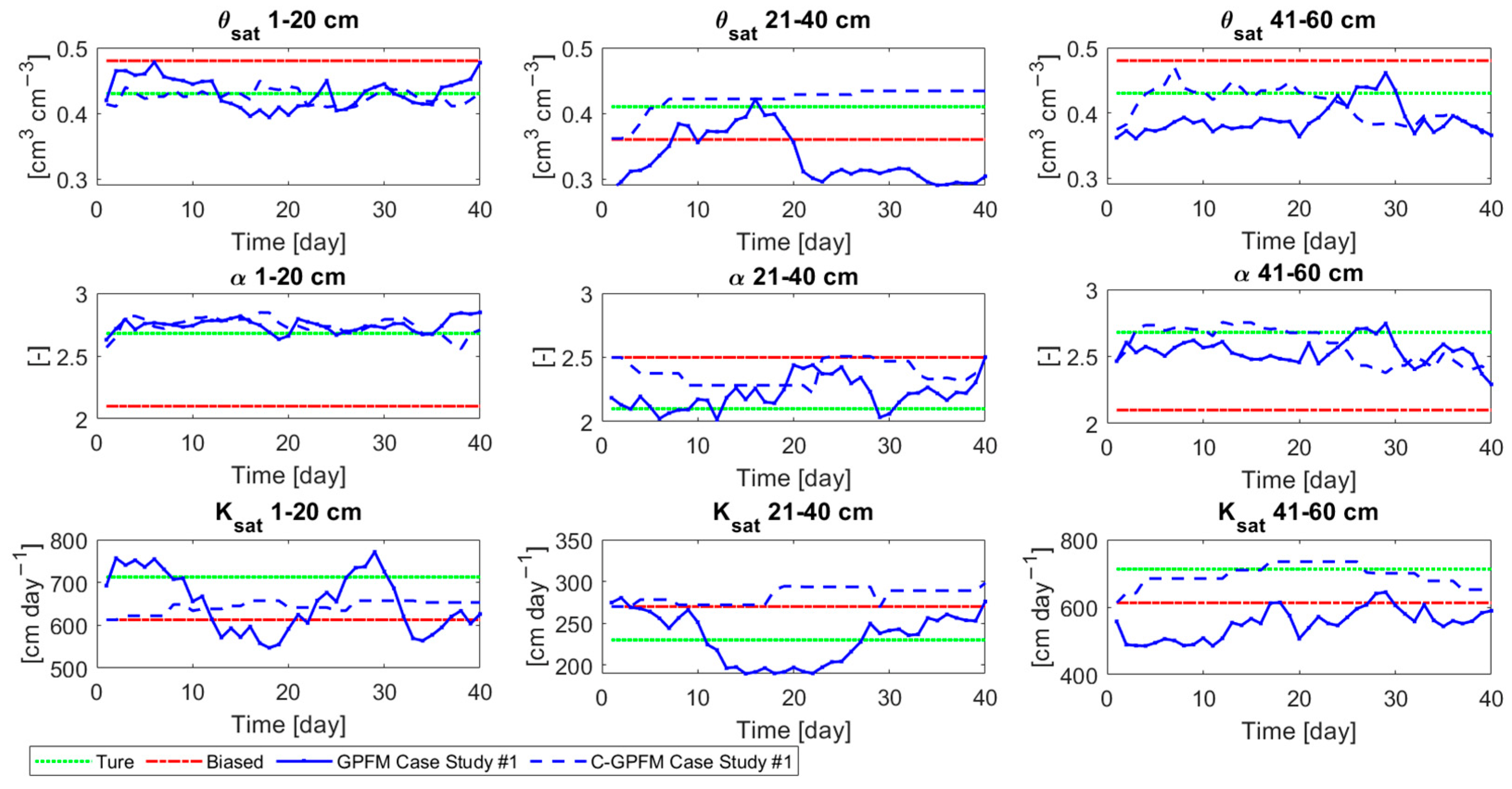
The ability of the model ensemble to accurately predict future variations of soil moisture depends directly on the accuracy of the parameter estimates, which can be appreciated from Figure 3. In this figure, the average of the parameters estimation (posterior) at each time step is presented. In most of the time steps, the estimation of the parameters in C-GPFM is improved compared to the ’biased’ (no assimilation) case. More importantly, the estimations of C-GPFM are superior and more consistent than GPFM. This can be attributed to the fact that when a parameter is non-influential, C-GPFM does not involve it in the assimilation process. For example, the parameters of the middle layer are less correlated with the measurements than the other parameters, which was to be expected since measurements were performed only in the top and bottom layers. Therefore, the estimation of the middle layer parameters by GPFM is erratic and inconsistent. By comparison, when applying C-GPFM, these parameters remain mostly constant as they are rarely involved in the data assimilation procedure. Overall, the estimations of a and θsat were better than Ksat in both methods due to the high influence of these parameters on the water content [21]. However, the estimations of θsat by C-GPFM are superior to GPFM at the middle layer.
Despite the intensive precipitation amounts, the water content was around 0.14, which is closer to the dryness than to the saturation. In such situations, the sensitiveness of the near-dryness influencing parameters is greater than those of the near-saturation, hence the improvements in these influencing parameters [27]. Therefore, a is estimated more accurately than the other parameters. For stronger enhancement of the other parameters, wetter soil should be used, which would be the case in heavier soils (e.g., clay) or with less permeable lower boundaries.
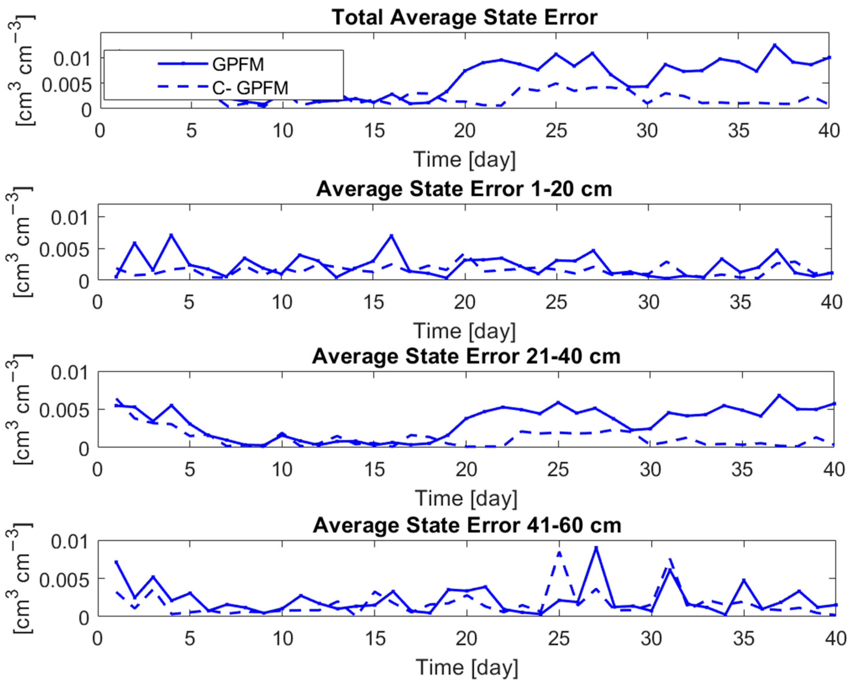
The accuracy of the estimation of the parameters is reflected on the estimation of the current state, i.e., water content (Figure 4). The top frame shows the absolute estimation error integrated over the whole soil profile (averaged over the 100 models of the ensemble) while the other frames show the absolute estimation error at the middle of each layer (averaged over 1 cm depth). The consistency and accuracy of the C-GPFM can be clearly observed in all three layers. The most noticeable improvement is observed in the second layer, which agrees with the previous observation regarding the “stability” of the parameter estimations in that layer (Figure 3).
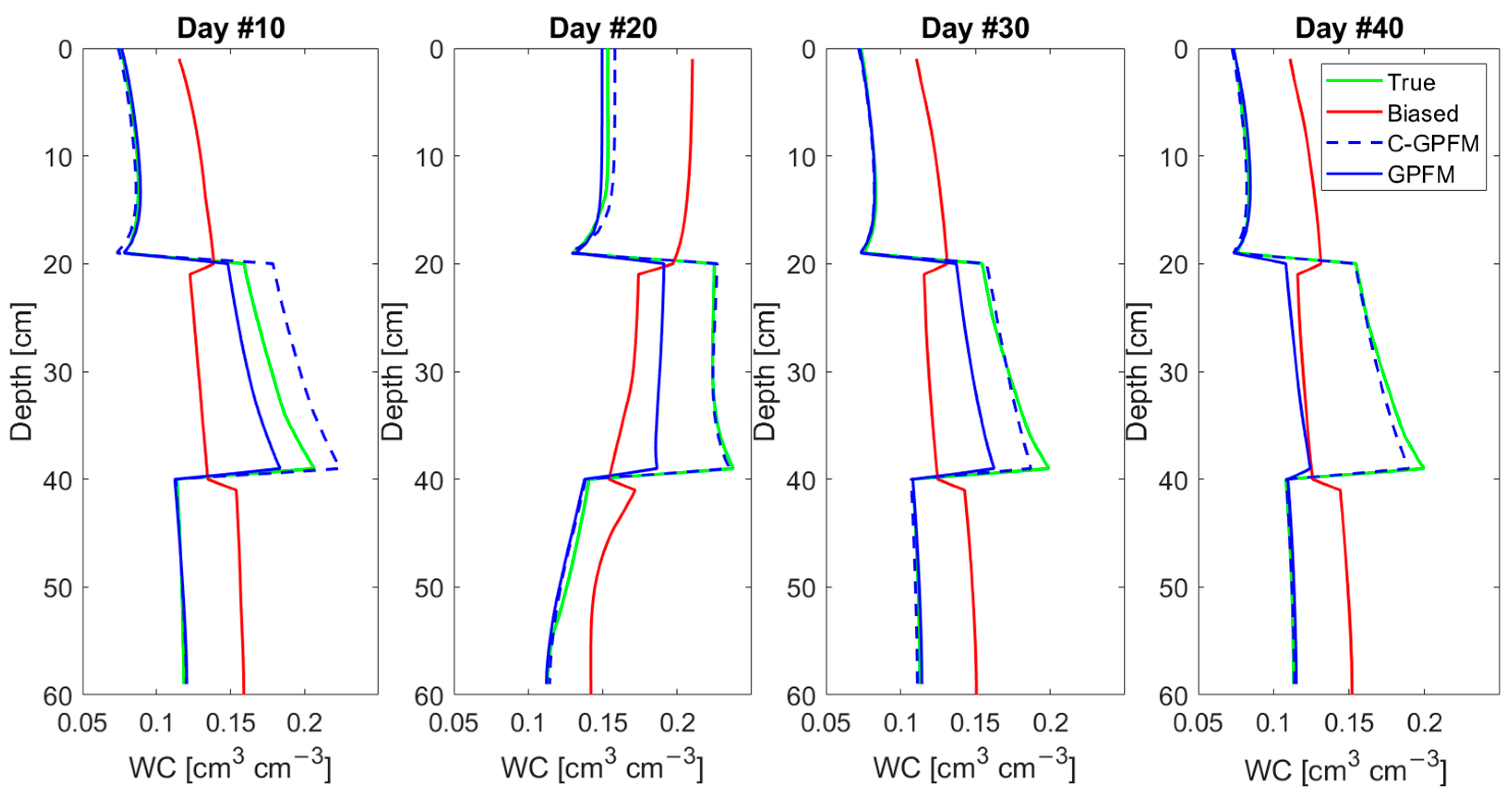
The superiority of C-GPFM in estimating the whole moisture profile is further demonstrated in Figure 5, which shows snapshots at selected days. The main advantage of C-GPFM is at the mid-layer although C-GPFM is also slightly better at the other layers. In addition, the estimates obtained by C-GPFM are consistently improved, while the results obtained by GPFM are not consistent.
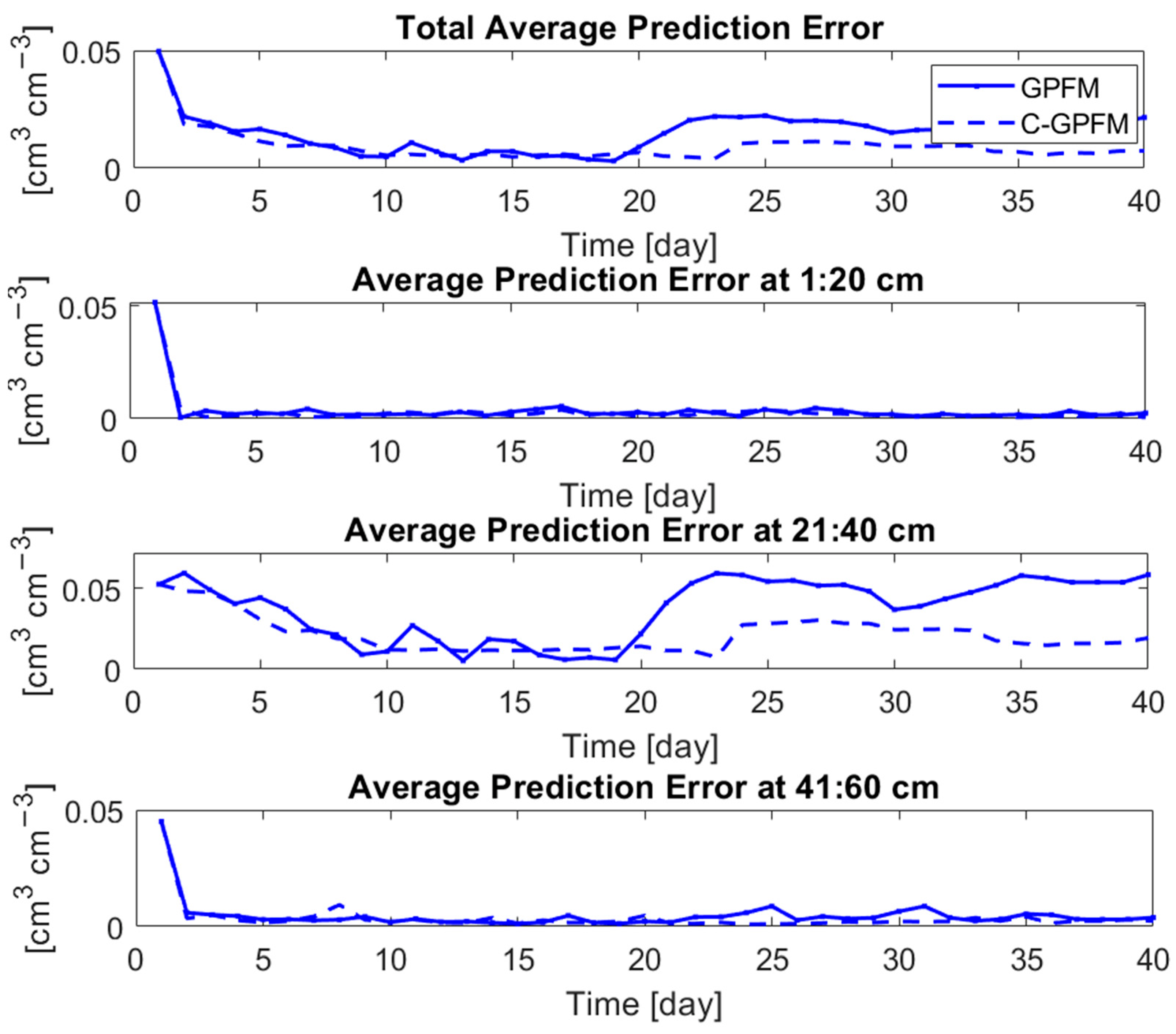
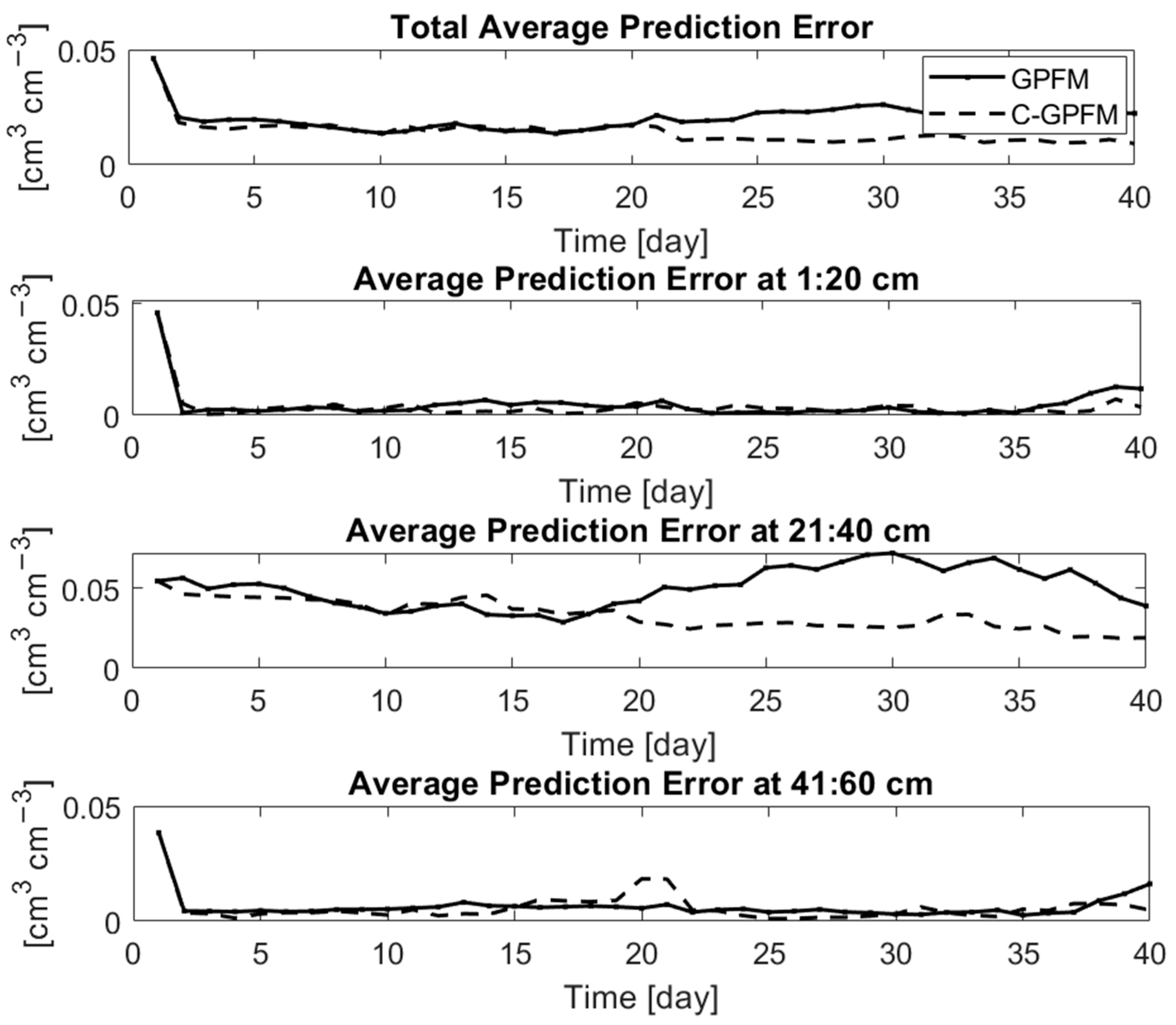
The ability of the data-assimilated models to accurately predict soil moisture evolution in response to future precipitation events was further tested as follows. At each assimilation day, the average ensemble of posterior parameters was used to predict the soil water content for the next 20 days. The results are shown in Figure 6. Compared to GPFM, C-GPFM improved the prediction accuracy in the middle layer significantly, and this improvement remained quite stable throughout the whole period. By comparison, starting from day 20 there is a significant degradation of the predictions of GPFM. This agrees with the degradation in the current state estimation observed in Figure 4 and Figure 5. The estimation for the top and bottom layers were good in all methods due to the improved estimations of the current state (Figure 4) and parameters (Figure 3). Notably, despite the inconsistent improvement in the saturated hydraulic conductivity and saturated soil moisture (Figure 3), the accuracy of the prediction is still accurate. This is due to the low influence of these parameters in the prediction period, in which the soil moisture is similar to the residual water content.
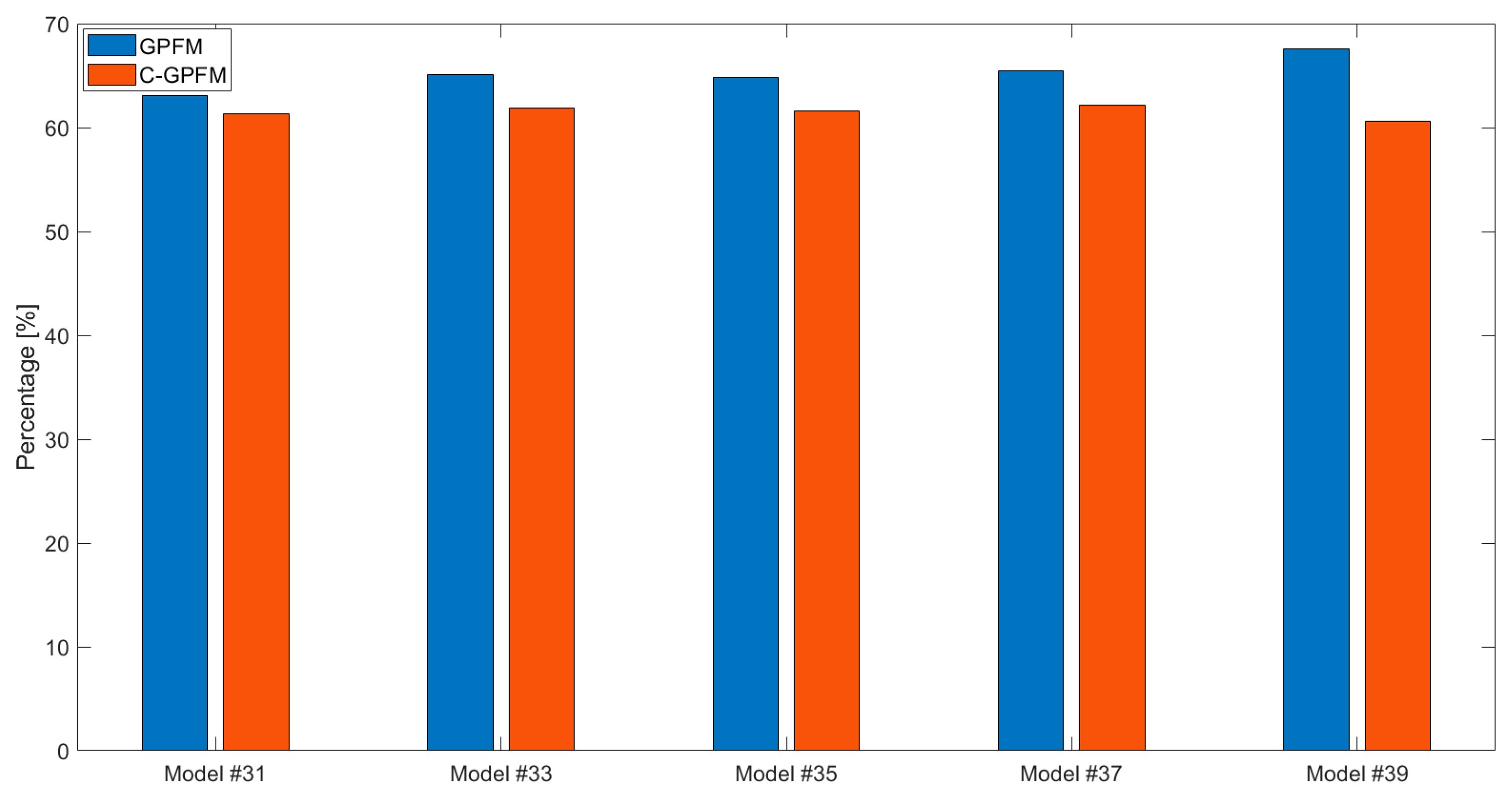
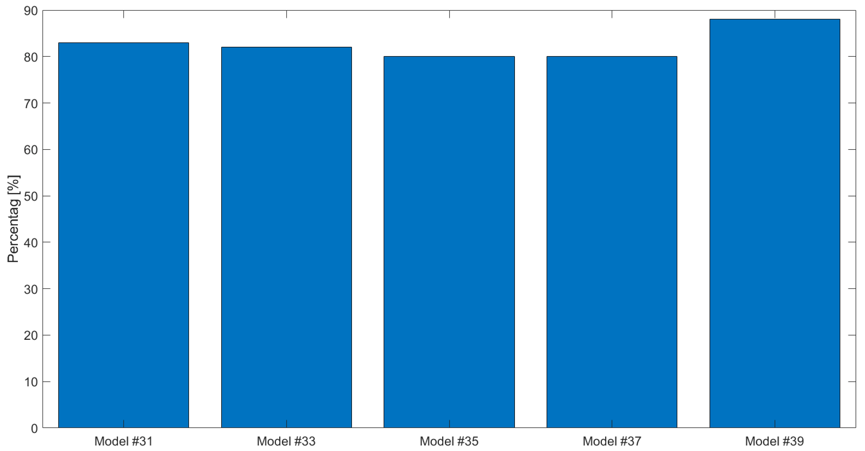
In order to neutralize the effect of the current state on future predictions and test solely the impact of parameters estimations on predictions, an additional test was conducted. In this test, on each assimilation day, the average of the set of the posterior parameters was used to predict the soil water content for a 20-day period. To test the robustness of the methods under different initial conditions and different irrigation schedules, one hundred runs were conducted, in which the initial conditions were set as the true values corrupted by white Gaussian noise with a standard deviation of 10%. In addition, the probability of precipitation on each day was set to 50% and the precipitation amount on those days was sampled from a uniform distribution between 0 and 10 cm. The error (averaged over time, depth and runs) of the ensemble at days 31, 33, 35, 37 and 39, normalized with respect to the ’biased’ model error on the same day is presented in Figure 7. Compared to the ’biased’ model (no assimilation), both assimilation approaches (GPFM and C-GPFM) reduced the prediction errors by about 40%. However, C-GPFM is 5–10% more accurate than GPFM in all of the time steps. Figure 8, which shows the percentage of runs in which C-GPFM outperformed GPFM, shows that C-GPFM performed better than GPFM not only on average but also on the vast majority of single runs (about 80% of the runs).
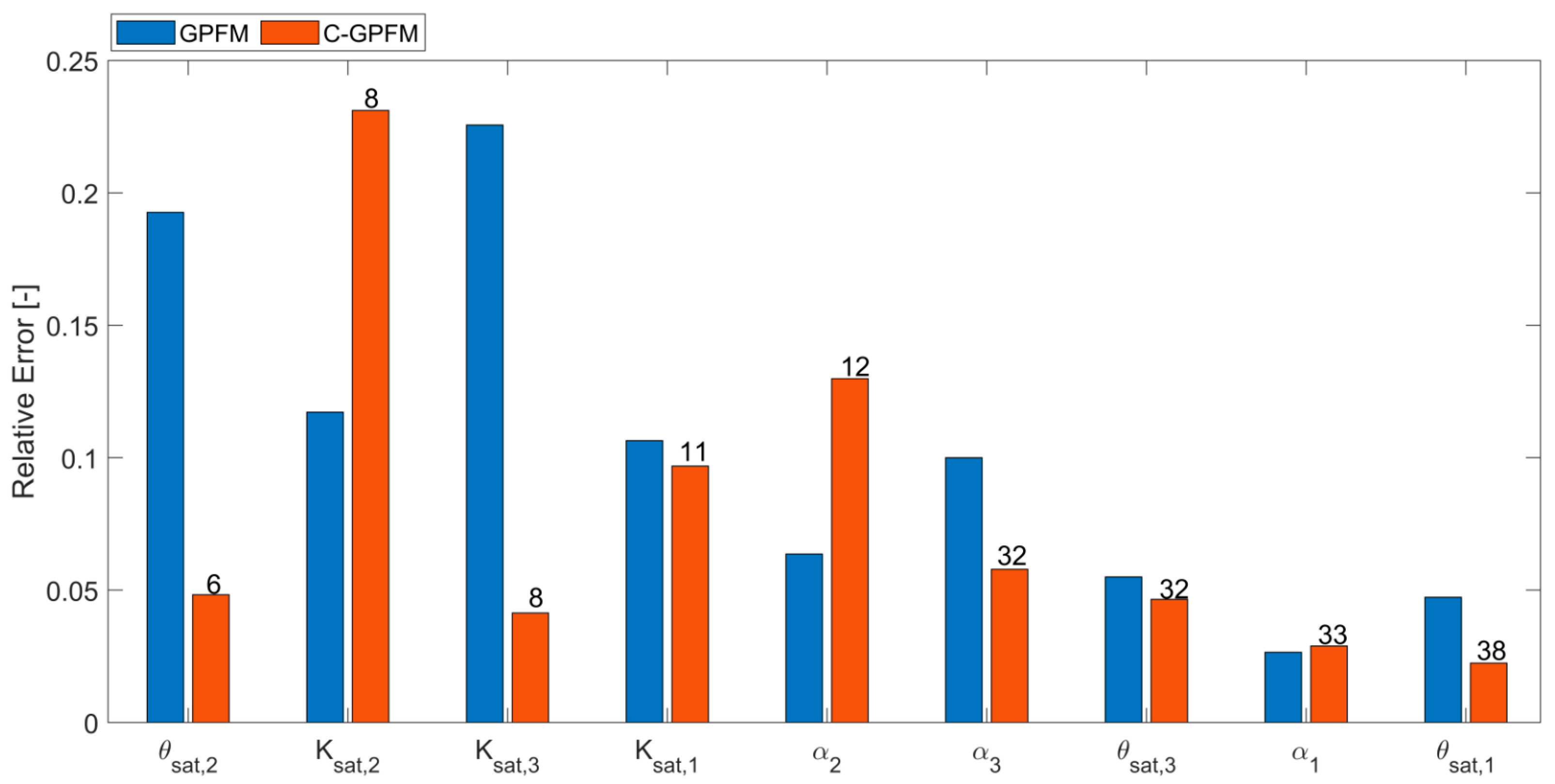
The superiority of the C-GPFM over GPFM stems only from the dynamic selection of specific parameters according to their correlation with the available measurements. In order to further investigate the relation between the accuracy of parameter estimation and selection frequency (i.e., parameter influence), the relative absolute error of each parameter (averaged over time) was plotted after sorting the parameters according to the number of times they were selected for adjustment (Figure 9). In addition, the number of times the parameter was selected for adjustment by C-GPFM is presented on the top of the figure. The relative error obtained by GPFM is also shown for comparison. Overall, the parameters selected more frequently are estimated more accurately than the parameters selected less frequently, which validates the motivation for the proposed approach, namely that the more strongly a parameter is correlated with measurements, the more influential the parameter is, and the more its estimation can be improved. As shown previously, the superiority of C-GPFM over GPFM in estimating most of the parameters is clear. Again, overall, the shape parameter is more accurate than the others using both methods, as the soil moisture is closer to the residual water content than to the saturated water content.
4.2. Case Study #2—Cyclic Boundary Condition
The general trend of the results was similar to that observed in Case Study #1. Since the irrigation applied was lower than in Case Study #1, in which the soil moisture was close to residual water content (Figure 5), the soil moisture was also close to residual water content here. Therefore, similarly to Case Study #1, the estimation of the saturated water content and the saturated hydraulic conductivity did not follow any clear trend and did not converge. Hence, the main difference between the two case studies is reflected in the estimation of , which is presented and discussed below. For brevity, only the ability of the ensemble to predict soil moisture in response to future wetting events and the estimations of are presented and discussed below. Figure 10 shows the average prediction accuracy of each ensemble when used to predict soil moisture for the next 20 days. Similar to Figure 6, this figure shows the overall prediction error as well as the prediction error for each layer, both for C-GPFM and GPFM. The superiority of C-GPFM, mainly on the mid-layer, agrees with the results of Case Study #1 (Figure 6). In particular, it is interesting to observe the results of the models that have been adjusted using at least one full wetting-drying cycle, i.e., the models obtained from Day 20 onward: clearly, the model obtained by C-GPFM is able to predict the evolution of soil moisture during the second and third wetting-drying cycles much more accurately.
In this case study, in contrast to case study #1, the influence of the soil parameters is cyclic following the cyclic nature of the wetting–drying periods. The influence of parameters such as saturated hydraulic conductivity and saturated water content is high during near saturation periods, while other parameters such as the shape parameters are more influential during near dry periods [27]. Therefore, in cases where the water content is near saturation or residual water content, the corresponding parameters are be improved. As mentioned, in this case study the water content was not near saturation during the wetting periods (days 1–10, 21–30), but the water content was near residual water content during the drying periods (days 11–20, 31–40). Therefore, when involving all the parameters (using GPFM), the shape parameter of is improved during the drying periods while worsening during the wetting periods. Since the soil moisture was not near saturation, the actual value of saturated hydraulic conductivity had little impact on the results and therefore could not be estimated accurately.
In Table 2, the absolute error ratio between the end and the beginning of each drying/wetting period at each layer is presented. Whenever this value is below 1, this indicates that there was an improvement of the parameter estimation during this period, and vice versa. During the drying periods, an improvement is observed in all the layers, while during the wetting periods the accuracy degrades. This behavior highlights that a parameter’s estimation improvement is conditional on its high sensitivity. At the bottom layer, this phenomenon is not as clear-cut since the bottom layer is wetter and farther from residual water content in comparison to the upper layers. This demonstrates the importance of using a quantitative approach for accurately identifying the influential parameters.
The multiplication of all error ratios provides an indication regarding the improvement during the total running period. As all the values are above 1, there is no improvement in the estimation of using GPFM. In contrast, using C-GPFM these multiplications are 0.98, 0.25 and 0.90 at the upper, middle and bottom layers, clearly showing very significant improvement for the middle layer. This emphasizes the advantage of performing real-time estimation of the parameters’ influence together with data assimilation.
5. Conclusions
This study presented a novel particle filter in which only a subset of the parameters was adjusted at each data assimilation step. The selection of the parameters was achieved by correlation analysis rather than sensitivity analysis in order to avoid a high computation burden. Using correlations for identifying the influential parameters was used as an alternative to sensitivity analysis techniques. Genetic-operator-based PF with Monte Carlo Markov Chain (based on [13]) was used as the data assimilation technique. The uniqueness of the proposed method is the ability to identify the highly influential parameters dynamically and in real-time with only marginal additional computational costs. The proposed method was applied to a water flow model (Hydrus-1D) in which states (soil water contents) and parameters (soil hydraulic parameters) were updated via data assimilation. Overall, the proposed method yielded state estimates and parameter estimates that were more accurate and more robust (consistent) than those obtained when adjusting all the parameters at each data assimilation step. The shape parameter was significantly improved during drying periods and in dry layers. Parameters highly sensitive near saturation conditions were less significantly improved when the soil was far from saturation, even during wetting periods. Therefore, designing experiments with near saturation and near residual water content is crucial for fast and good convergence of the parameters’ estimates. For further applications, this method could be used for designing experiments in such a way that small sub-sets of influential parameters are estimated efficiently in sequential periods.
Author Contributions
A.J. wrote the code, prepared the case studies, analyzed the results, and wrote the manuscript. R.L. contributed to the analysis of the results and reviewed the different versions of the manuscript. All authors have read and agreed to the published version of the manuscript.
Funding
The funding received from BARD, the United States—Israel Binational Agricultural Research and Development Fund, to carry out this research work is sincerely acknowledged.
Data Availability Statement
Not applicable.
Conflicts of Interest
The authors declare no conflict of interest.
References
- Simunek, J.; Sejna, M.; Van Genuchten, M.T.; Šimůnek, J.; Šejna, M.; Jacques, D.; Sakai, M. HYDRUS-1D. Simulating the one-Dimensional Movement of Water, Heat, and Multiple Solutes in Variably-Saturated Media. 1998. Version 2. Available online: https://www.pc-progress.com/en/Default.aspx?hydrus-1d (accessed on 1 October 2022).
- Das, N.N.; Mohanty, B.P. Root zone soil moisture assessment using passive microwave remote sensing and vadose zonemodeling. Vadose Zone J. 2006, 5, 296–307. [Google Scholar] [CrossRef] [Green Version]
- Das, N.N.; Mohanty, B.P.; Cosh, M.H.; Jackson, T.J. Modeling and assimilation of root zone soil moisture using remote sensing observations in Walnut Gulch watershed during SMEX04. Remote Sens. Environ. 2008, 112, 415–429. [Google Scholar] [CrossRef]
- Brandhorst, N.; Erdal, D.; Neuweiler, I. Soil moisture prediction with the ensemble Kalman filter: Handling uncertainty of soil hydraulic parameters. Adv. Water Res. 2017, 110, 360–370. [Google Scholar] [CrossRef]
- Abbaszadeh, P.; Moradkhani, H.; Yan, H. Enhancing hydrologic data assimilation by evolutionary particle filter and Markov chain Monte Carlo. Adv. Water Res. 2018, 111, 192–204. [Google Scholar] [CrossRef]
- Bauser, H.H.; Berg, D.; Klein, O.; Roth, K. Inflation method for ensemble Kalman filter in soil hydrology. Hydrol. Earth Syst. Sci. 2018, 22, 4921–4934. [Google Scholar] [CrossRef] [Green Version]
- Berg, D.; Bauser, H.H.; Roth, K. Covariance resampling for particle filter–state and parameter estimation for soil hydrology. Hydrol. Earth Syst. Sci. 2019, 23, 1163–1178. [Google Scholar] [CrossRef] [Green Version]
- Jamal, A.; Linker, R. Inflation method based on confidence intervals for data assimilation in soil hydrology using ensemble Kalman filter. Vadose Zone J. 2020, 19, e20000. [Google Scholar] [CrossRef] [Green Version]
- Reichle, R.H.; McLaughlin, D.B.; Entekhabi, D. Hydrologic data assimilation with the ensemble Kalman filter. Mon. Weather Rev. 2002, 130, 103–114. [Google Scholar] [CrossRef]
- De Lannoy, G.J.; Reichle, R.H.; Houser, P.R.; Pauwels, V.R.; Verhoest, N.E. Correcting for forecast bias in soil moisture assimilation with the ensemble Kalman filter. Water Resour. Res. 2007, 43, 117. [Google Scholar] [CrossRef] [Green Version]
- DeChant, C.M.; Moradkhani, H. Examining the effectiveness and robustness of sequential data assimilation methods for quantification of uncertainty in hydrologic forecasting. Water Resour. Res. 2012, 48, 136. [Google Scholar] [CrossRef]
- Yin, S.; Zhu, X. Intelligent particle filter and its application to fault detection of nonlinear system. IEEE Trans. Ind. Electron. 2015, 62, 3852–3861. [Google Scholar] [CrossRef]
- Jamal, A.; Linker, R. Genetic Operator-Based Particle Filter Combined with Markov Chain Monte Carlo for Data Assimilation in a Crop Growth Model. Agriculture 2020, 10, 606. [Google Scholar] [CrossRef]
- Moradkhani, H.; Hsu, K.L.; Gupta, H.; Sorooshian, S. Uncertainty assessment of hydrologic model states and parameters: Sequential data assimilation using the particle filter. Water Resour. Res. 2005, 41, 480. [Google Scholar] [CrossRef] [Green Version]
- Moradkhani, H.; DeChant, C.M.; Sorooshian, S. Evolution of ensemble data assimilation for uncertainty quantification using the particle filter-Markov chain Monte Carlo method. Water Resour. Res. 2012, 48, 162. [Google Scholar] [CrossRef]
- Andrieu, C.; Doucet, A.; Holenstein, R. Particle markov chain monte carlo methods. J. R. Stat. Soc. Ser. B 2010, 72, 269–342. [Google Scholar] [CrossRef] [Green Version]
- Kroes, J.G.; Van Dam, J.C.; Bartholomeus, R.P.; Groenendijk, P.; Heinen, M.; Hendriks, R.F.A.; Van Walsum, P.E.V. SWAP Version 4 (No. 2780). Wageningen Environmental Research. 2017. Available online: https://research.wur.nl/en/publications/swap-version-4 (accessed on 1 October 2022).
- Hamby, D.M. A review of techniques for parameter sensitivity analysis of environmental models. Environ. Monit. Assess. 1994, 32, 135–154. [Google Scholar] [CrossRef]
- Della Peruta, R.; Keller, A.; Schulin, R. Sensitivity analysis, calibration and validation of EPIC for modelling soil phosphorus dynamics in Swiss agro-ecosystems. Environ. Model. Softw. 2014, 62, 97–111. [Google Scholar] [CrossRef]
- Wu, M.; Ran, Y.; Jansson, P.E.; Chen, P.; Tan, X.; Zhang, W. Global parameters sensitivity analysis of modeling water, energy and carbon exchange of an arid agricultural ecosystem. Agric. For. Meteorol. 2019, 271, 295–306. [Google Scholar]
- Xu, X.; Sun, C.; Huang, G.; Mohanty, B.P. Global sensitivity analysis and calibration of parameters for a physically-based agro-hydrological model. Environ. Model. Softw. 2016, 83, 88–102. [Google Scholar] [CrossRef] [Green Version]
- De Pue, J.; Rezaei, M.; Van Meirvenne, M.; Cornelis, W.M. The relevance of measuring saturated hydraulic conductivity: Sensitivity analysis and functional evaluation. J. Hydrol. 2019, 576, 628–638. [Google Scholar] [CrossRef]
- Claverie, M.; Demarez, V.; Duchemin, B.; Hagolle, O.; Ducrot, D.; Marais-Sicre, C.; Dedieu, G. Maize and sunflower biomass estimation in southwest France using high spatial and temporal resolution remote sensing data. Remote Sens. Environ. 2012, 124, 844–857. [Google Scholar] [CrossRef]
- Linker, R.; Kisekka, I. Concurrent data assimilation and model-based optimization of irrigation scheduling. Agric. Water Manag. 2022, 274, 107924. [Google Scholar] [CrossRef]
- Zhang, T.; Su, J.; Liu, C.; Chen, W.H. State and parameter estimation of the AquaCrop model for winter wheat using sensitivity informed particle filter. Comput. Electron. Agric. 2021, 180, 105909. [Google Scholar] [CrossRef]
- Manache, G.; Melching, C.S. Identification of reliable regression-and correlation-based sensitivity measures for importance ranking of water-quality model parameters. Environ. Model. Softw. 2008, 23, 549–562. [Google Scholar] [CrossRef]
- Shun, H.; Shi, L.; Huang, K.; Zha, Y.; Hu, X.; Ye, H.; Yang, Q. Improvement of sugarcane crop simulation by SWAP-WOFOST model via data assimilation. Field Crops Res. 2019, 232, 49–61. [Google Scholar]
- Gordon, N.J.; Salmond, D.J.; Smith, A.F. Novel approach to nonlinear/non-Gaussian Bayesian state estimation. IEE Proc. F (Radar Signal Process.) 1993, 140, 107–113. [Google Scholar] [CrossRef] [Green Version]
- Carpenter, J.; Clifford, P.; Fearnhead, P. Improved particle filter for nonlinear problems. IEE Proc. -Radar Sonar Navig. 1999, 146, 2–7. [Google Scholar] [CrossRef]
- Kitagawa, G. Monte Carlo filter and smoother for non-Gaussian nonlinear state space models. J. Comput. Graph. Stat. 1996, 5, 1–25. [Google Scholar]
- Asuero, A.G.; Sayago, A.; González, A.G. The correlation coefficient: An overview. Crit. Rev. Anal. Chem. 2006, 36, 41–59. [Google Scholar] [CrossRef]
- Rocha, D.; Abbasi, F.; Feyen, J. Sensitivity analysis of soil hydraulic properties on subsurface water flow in furrows. J. Irrig. Drain. Eng. 2006, 132, 418–424. [Google Scholar] [CrossRef]
- Schaap, M.G.; Leij, F.J.; Van Genuchten, M.T. Rosetta: A computer program for estimating soil hydraulic parameters with hierarchical pedotransfer functions. J. Hydrol. 2001, 251, 163–176. [Google Scholar] [CrossRef]
- Akoglu, H. User’s guide to correlation coefficients. Turk. J. Emerg. Med. 2018, 18, 91–93. [Google Scholar] [CrossRef] [PubMed]
Figure 1.
The overall framework including stages A–G.

Figure 2.
Precipitation/irrigation (boundary condition) in Case Study #1 and Case Study #2.

Figure 3.
Average of parameters posteriors by C-GPFM and GPFM together with the ‘true’ and ‘biased’ values for Case Study #1.
Figure 3.
Average of parameters posteriors by C-GPFM and GPFM together with the ‘true’ and ‘biased’ values for Case Study #1.

Figure 4.
Average of state posteriors by C-GPFM and GPFM in Case Study #1.

Figure 5.
Average of parameters posteriors by C-GPFM and GPFM at days #10, #20, #30 and #40 for Case Study #1.
Figure 5.
Average of parameters posteriors by C-GPFM and GPFM at days #10, #20, #30 and #40 for Case Study #1.

Figure 6.
Average of state prediction error for the next 20 days at each day of assimilation by C-GPFM and GPFM for Case Study #1.
Figure 6.
Average of state prediction error for the next 20 days at each day of assimilation by C-GPFM and GPFM for Case Study #1.

Figure 7.
State posterior errors (averaged over time, depth and runs) normalized with respect to the error of the biased (no assimilation) model. Results for the models obtained on days #31, #33, #35, #37 and #39 by C-GPFM and GPFM for Case Study #1.
Figure 7.
State posterior errors (averaged over time, depth and runs) normalized with respect to the error of the biased (no assimilation) model. Results for the models obtained on days #31, #33, #35, #37 and #39 by C-GPFM and GPFM for Case Study #1.

Figure 8.
Percentage of the runs in which C-GPFM led to smaller average state errors than GPFM. Results for the models obtained on days #31, #33, #35, #37 and #39 for Case Study #1.
Figure 8.
Percentage of the runs in which C-GPFM led to smaller average state errors than GPFM. Results for the models obtained on days #31, #33, #35, #37 and #39 for Case Study #1.

Figure 9.
Relative absolute error of each parameter (averaged over time) estimated by C-GPFM and GPFM together with the number of times the parameter was selected for adjustment by C-GPFM for Case Study #1. The number of times a parameter was selected for adjustment by C-GPFM is indicated above the corresponding sack.

Figure 10.
Average of state prediction error for the next 20 days at each day of assimilation by C-GPFM and GPFM for Case Study #2.
Figure 10.
Average of state prediction error for the next 20 days at each day of assimilation by C-GPFM and GPFM for Case Study #2.


Table 1.
The soil parameters used in the case studies.
| Parameter | Description | Depth | ‘True’ | ‘Biased’ |
|---|---|---|---|---|
| Saturated water content | 0–20 cm 21–40 cm 41–60 cm | 0.43 0.41 0.43 | 0.48 0.36 0.48 | |
| Air entrance value parameters | 0–20 cm 21–40 cm 41–60 cm | 2.68 2.10 2.68 | 2.1 2.5 2.1 | |
| 0–20 cm 21–40 cm 41–60 cm | 713 230 713 | 613 270 613 | ||
| Residual water content | 0–20 cm 21–40 cm 41–60 cm | 0.045 0.061 0.045 | ||
| Shape parameter | 0–20 cm 21–40 cm 41–60 cm | 0.14 0.10 0.14 | ||
Table 2.
The absolute error ratio of the parameter between the end and the beginning of the drying and wetting periods using GPFM.
Table 2.
The absolute error ratio of the parameter between the end and the beginning of the drying and wetting periods using GPFM.
| Period | 0–20 cm Layer | 21–40 cm Layer | 41–60 cm Layer |
|---|---|---|---|
| Days 1–10 (wetting) | 2.63 | 1.42 | 0.71 |
| Days 11–20 (drying) | 0.36 | 0.24 | 0.77 |
| Days 21–30 (wetting) | 1.52 | 11.6 | 2.62 |
| Days 31–40 (drying) | 0.78 | 0.72 | 1.39 |
| Ratios Multiplication | 1.12 | 2.85 | 1.99 |
Publisher’s Note: MDPI stays neutral with regard to jurisdictional claims in published maps and institutional affiliations. |
© 2022 by the authors. Licensee MDPI, Basel, Switzerland. This article is an open access article distributed under the terms and conditions of the Creative Commons Attribution (CC BY) license (https://creativecommons.org/licenses/by/4.0/).
Share and Cite
MDPI and ACS Style
Jamal, A.; Linker, R. Covariance-Based Selection of Parameters for Particle Filter Data Assimilation in Soil Hydrology. Water 2022, 14, 3606. https://doi.org/10.3390/w14223606
AMA Style
Jamal A, Linker R. Covariance-Based Selection of Parameters for Particle Filter Data Assimilation in Soil Hydrology. Water. 2022; 14(22):3606. https://doi.org/10.3390/w14223606
Chicago/Turabian StyleJamal, Alaa, and Raphael Linker. 2022. "Covariance-Based Selection of Parameters for Particle Filter Data Assimilation in Soil Hydrology" Water 14, no. 22: 3606. https://doi.org/10.3390/w14223606
Note that from the first issue of 2016, this journal uses article numbers instead of page numbers. See further details here.