Hydrologic Performance of Low Impact Developments in a Cold Climate

Abstract

The application of the low impact development (LID) in a cold climate such as northeastern China is constrained by two unresolved research questions with regards to its infiltration potential through the winter and its varied runoff regimes between winters and summers. This study picked a typical residential district under construction in Changchun, China, and modeled the storm drainage system with and without LID facilities based on the Storm Water Management Model. The hydrological performance of LID was evaluated through various design storms and historic rain events in dry, average, and wet years. The influence of the Horton and the Green–Ampt infiltration methods on the seasonal water budgets was particularly compared since the former is universally adopted in China while the latter is more widely used in the U.S. and other countries. The results indicate that the Horton method tended to generate a higher infiltration volume than the Green–Ampt method. Consequently, when driven by the 100-year design storm, the Horton method led to a 17.4% higher outflow than the Green–Ampt method; when driven by the measured 3-year precipitation in the study area, the yearly runoff coefficients, with regards to the Horton method, were at least 1.3 times higher than those modeled by the Green–Ampt method. This finding challenged the interchangeable use of the Horton and Green–Ampt methods without tests. Furthermore, the formation of snow covers in winter also reduced the permeability of LID and its capacity of managing runoff compared to summer. However, LID still exhibited a decent potential of regulating the winter runoff in the cold region compared to the baseline, possibly owing to the presence of frequent freezing-thawing cycles.

1. Introduction

During rapid urbanization, especially in China, many naturally pervious surfaces have been replaced by impermeable materials, such as concrete and asphalt, leading to a significant increase in surface runoff, shorter confluence time, earlier flood peaks, and the related environmental problems [1]. Currently, flooding has become a major urban threat after population congestion, traffic congestion, and environmental pollution [2,3]. Meanwhile, rainwater as an alternative irrigation supply is often not utilized at the source location, and many cities still face the challenge of water shortage, where the philosophy of traditional stormwater management needs to be updated. The ‘sponge city’ policy was, therefore, proposed in China in April 2012 [2], which adopted low impact development (LID), green infrastructure, sustainable urban drainage system, and other similar concepts, to manage stormwater runoff and restore the predevelopment condition [4,5].

While the concept of LID has been widely adopted by many countries, the research on the hydrologic performance of the LID in a cold climate is relatively lacking, with considerable uncertainty about the effect of freeze-thaw cycles on osmosis [6]. For example, the permeability of cohesive silty soils was found to increase with the number of freeze-thaw cycles [7], whereas in loam and cohesive soils, the permeability remained unchanged or slightly decreased [8]. The effectiveness of LID facilities in treating and reducing surface runoff largely depends on their permeability [9]. Meanwhile, studies have shown that surfaces with dense vegetation (such as grass) tend to maintain low soil water content and high permeability, and do not easily form frost [10]. These all increase the uncertainty for the design, layout, and drainage process of the LID facilities in cold regions.

A few studies of the snowmelt runoff generation based on the Storm Water Management Model (SWMM) have been conducted in regions and countries with seasonal snow covers [11,12,13]. Compared with storm runoff, snowmelt runoff differs in formation, peak time, and duration. In general, urban catchments release snowmelt storage at flow rates much lower than those sourced from high-intensity rainfall events, but the total volume of snowmelt runoff could still contribute to ponding and flooding in urban areas, especially during the rain-on-snow events [11,14]. While there are few relevant studies existing in China, a study showed that the snowmelt water took up a significant proportion of the spring runoff in the thawing stage [15]. However, the urban drainage system, including the LID, is usually designed only based on summer rainfall; the influence of the snowfall and snowmelt runoff is seldom considered and needs to be quantified.

Since evapotranspiration is usually not significant during the long winter, infiltration becomes the major loss term in the cold zone. Generally speaking, the Horton method has been widely used in China [16,17,18], possibly due to the lower requirements in the data inputs, while the Green–Ampt method is more widely used internationally in countries such as the U.S. Although the Horton and Green–Ampt methods were found to generate similar infiltrated volumes and peak flows for sandy and clay soils, the two methods behaved differently in the wetting process [19]. Given the dry period before the rain event, the peak rate and the runoff volume modeled by the Green–Ampt method were only 30%, and 11% of those modeled by the Horton method, indicating the potential of higher infiltration resulted from the former method [20]. In contrast, some researchers have used the Morris method to analyze the parameter sensitivity of the Horton and Green–Ampt methods and found that the standard deviation of the output of the Green–Ampt method was smaller than that of the Horton method [21,22]. The Green–Ampt model, though involving more parameters, was thought to be slightly more accurate than the Horton model in calculating infiltration rates, while the Horton model was easier to apply [23,24,25]. The relevant studies are extremely sparse for a cold climate, where freezing and thawing cycles could add more complexity.

The purpose of this research, therefore, was to compare the two infiltration methods applied in a cold environment, and to compare the capacity of the LID between the summer and winter. The results can be expected to guide the application of the LID in cold regions, such as northeastern China, and to provide the theoretical basis for evaluating the ‘sponge city’ or similar policies for cities in cold climates.

2. Study Area

The study area was selected at a residential community being built in Changchun, Jilin Province, China, covering a total area of 39,027.38 m², with a relatively flat topography slightly leaning from south to north. The study area has a temperate continental semi-humid monsoon climate with a long and cold winter. According to the Chinese weather network, the multi-year monthly average temperature in Changchun from November to March is below 0 °C and the annual average temperature is 4.6 °C. The coldest month is January, with a monthly average temperature of −15.1 °C. The hottest month is July, which has an average temperature of 23.1 °C. The annual precipitation is 600–700 mm, while rainfall mainly occurs in June, July, and August, which accounts for more than 60% of the annual precipitation. On 16 July 2017, two heavy rainstorms fell within 24 h in Changchun, causing severe waterlogging on many roads and posing a serious threat to transportation facilities and infrastructure; the heavy rainfall on 2 June 2021 resulted in 52 waterlogged spots within Changchun. Meanwhile, the Chinese Central Environmental Protection Inspectorate inspected Changchun in September 2021 and attributed the local combined sewer overflows accompanied with the problems of the smelly and black water bodies to the overdue retrofitting work for converting the combined sewer system into the separate sewer system.

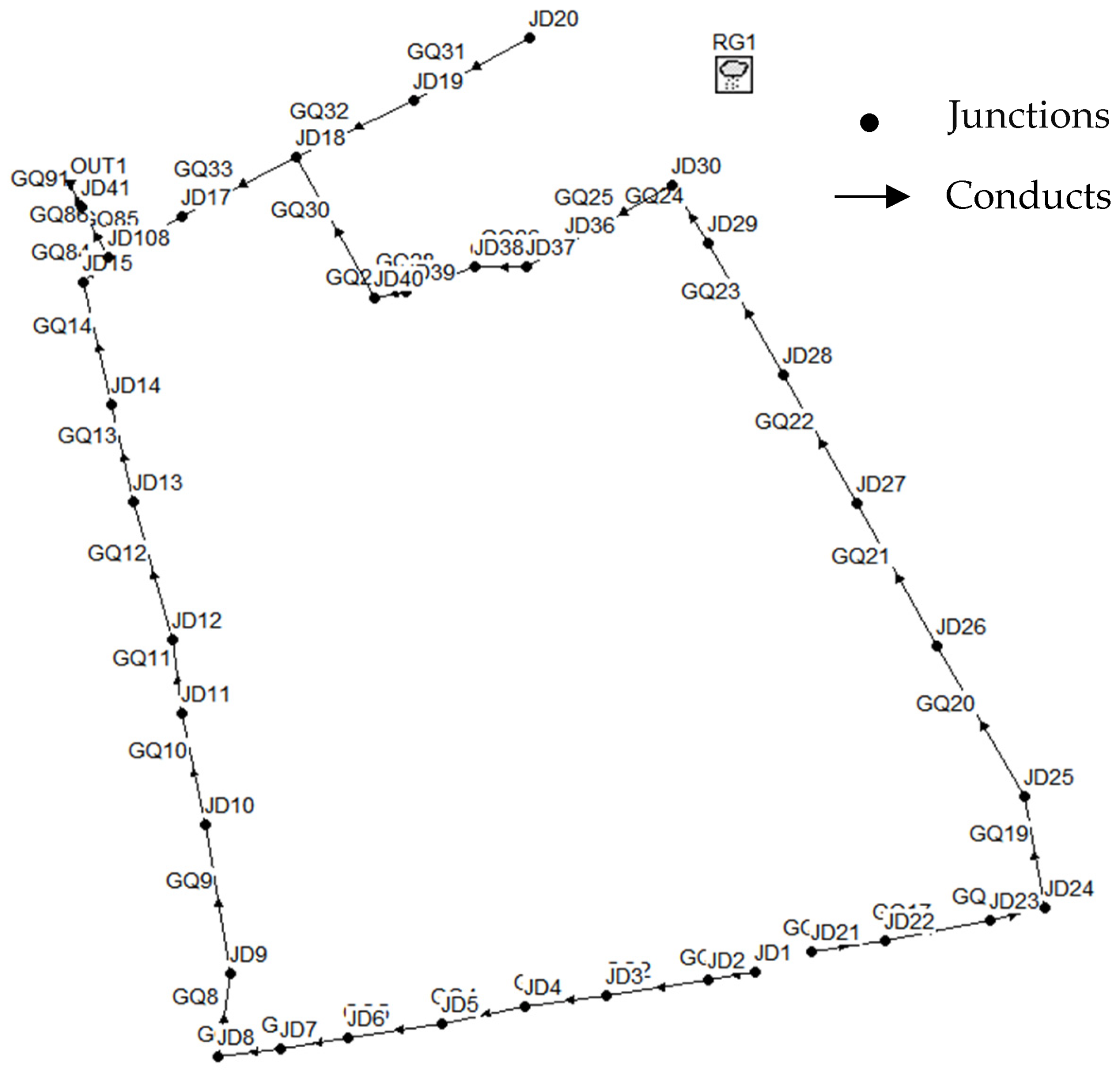
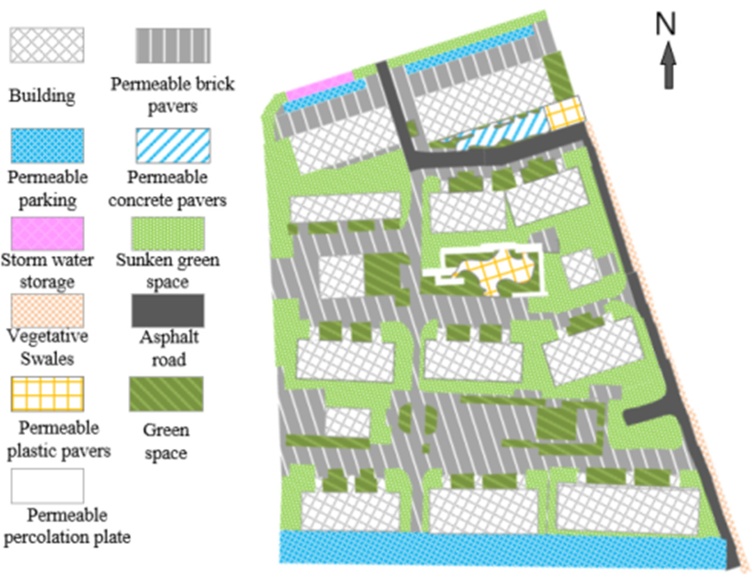
The required inputs mainly included hydrometeorological data, storm drainage networks, and surface settings, such as land use types. Most of the data were extracted from the architectural and drainage plans or were surveyed (Figure 1). The studied residential community adopted a separate sewer system, and the mainline lay along the major roads of the district. The landscape can be classified into 11 land use types, including buildings, green space, roads, permeable brick pavers, storm water storage modules, sunken green space, permeable parking spaces, permeable concrete pavers, permeable plastic pavers, vegetative swale, and permeable percolation plates (Figure 2). The historical time series of the local meteorological data, including rainfall, air temperature, and wind speed, were collected from the Chinese National Meteorological Information Center, which range from 2011 to 2020.

3. Methods

3.1. Calculation in SWMM

The SWMM was adopted by this study to simulate the urban precipitation-runoff process. The division between the rainfall and snowfall out of the precipitation was internally determined in SWMM by the 0 °C threshold given the temperature inputs. Both the Horton and Green–Ampt infiltration methods were used and compared. The SWMM uses Manning’s equation and the nonlinear reservoir method to model the runoff generation and transformation. The dynamic wave method was chosen to represent the non-constant flow phenomenon in the routing process [26,27].

The equation of the Horton method can be written as follows:

$$f_p=f_c+\left(f_0-f_c\right)e^{-kt}$$

(1)

where f_p is ground infiltration capacity (mm/h), f₀ is the initial infiltration capacity corresponding to the initial soil water content (mm/h), f_c is the stable infiltration rate, which is the infiltration capacity of soil when it reaches the field water capacity, k is the coefficient of infiltration capacity decreasing with time, and t is time (h).

The equation of the Green–Ampt method, proposed by Green and Ampt in 1911 [28,29], can be written as follows:

$$f_p=K_s[\frac{d+L_s+{\psi }_s}{L_s}]$$

(2)

where K_S is soil saturation water inflow coefficient (mm/h), d is the surface water depth (mm), L_S is the depth of wet front (mm), and ${\psi }_s$ is the suction force at the wet front (mm).

SWMM calculates the snowmelt rate by the energy balance method or the degree-day method depending on the presence of rainfall or not, which was intrinsically determined by the temperature threshold. In case of rain (the rain intensity must be greater than 0.51 mm/h), the energy balance method will be adopted as follows:

$$\mathrm{SMELT}=\left(0.001167+7.5{\mathsf{\gamma }\mathrm{U}}_{\mathrm{A}}+0.007\mathrm{i}\right)\left({\mathrm{T}}_{\mathrm{a}}-32\right)+8.5{\mathrm{U}}_{\mathrm{A}}\left({\mathrm{e}}_{\mathrm{a}}-0.18\right)$$

(3)

where $SMELT$ is the melting rate (in/h), $T_a$ is the air temperature (°F), $\gamma$ is the humidity constant (in Hg/°F), $U_A$ is the wind speed correction coefficient (in/in Hg-h), $i$ is rainfall intensity (in/h), and $e_a$ is the saturated vapor pressure temperature of air (Hg). This empirical formula and the equations listed afterward that also used the U.S. system of units were internally coded in SWMM but were later converted to the international system of units.

Without rainfall, the degree-day method will be adopted to calculate the snowmelt rate:

$$SMELT=DHM\left(T_a-Tbase\right)$$

(4)

where $SMELT$ is the melting rate (in/h), $Tbase$ is the base melting temperature (°F), and DHM is the melting coefficient (in/h-°F).

During simulation, the base temperature remains unchanged, yet the melting coefficient varies with the season according to the following equation:

$$DHM=\left(\frac{D_{MAX}+D_{MIN}}{2}\right)+\left(\frac{D_{MAX}-D_{MIN}}{2}\right)\sin \left(\frac{\pi }{182}\left(day-81\right)\right)$$

(5)

where D_MAX is the maximum snowmelt coefficient, which occurred on 21 June (in/h-°F), and D_MIN is the minimum snowmelt coefficient, which occurred on 21 December (in/h-°F), and day is the day of the year.

Snow is a porous medium like soil and has a certain “free-water holding capacity” before runoff generation starts. SWMM calculates the free-water holding capacity by the following formula [30]:

$$FWC=Fr\ast Swe$$

(6)

where FWC is free-water holding capacity (mm), Fr is a coefficient of snow depth (0.02–0.05), and Swe is the snow water equivalent (mm).

The Hargreaves method was used to compute evaporation rates depending on the daily maximal and minimum air temperatures [28]:

$$E=0.0023\left(\frac{R_a}{\lambda }\right)T_r{}^{\frac{1}{2}}\left(T_a+17.8\right)$$

(7)

where E is evaporation rate (mm/day), R_a is the water equivalent of incoming extraterrestrial radiation (MJ m⁻² d⁻¹), T_r is the average daily temperature range for a period of days (deg C), T_a is the average daily temperature for a period of days (deg C), and λ = 2.50−0.002361T_a is the latent heat of vaporization (MJ kg⁻¹).

3.2. Precipitation

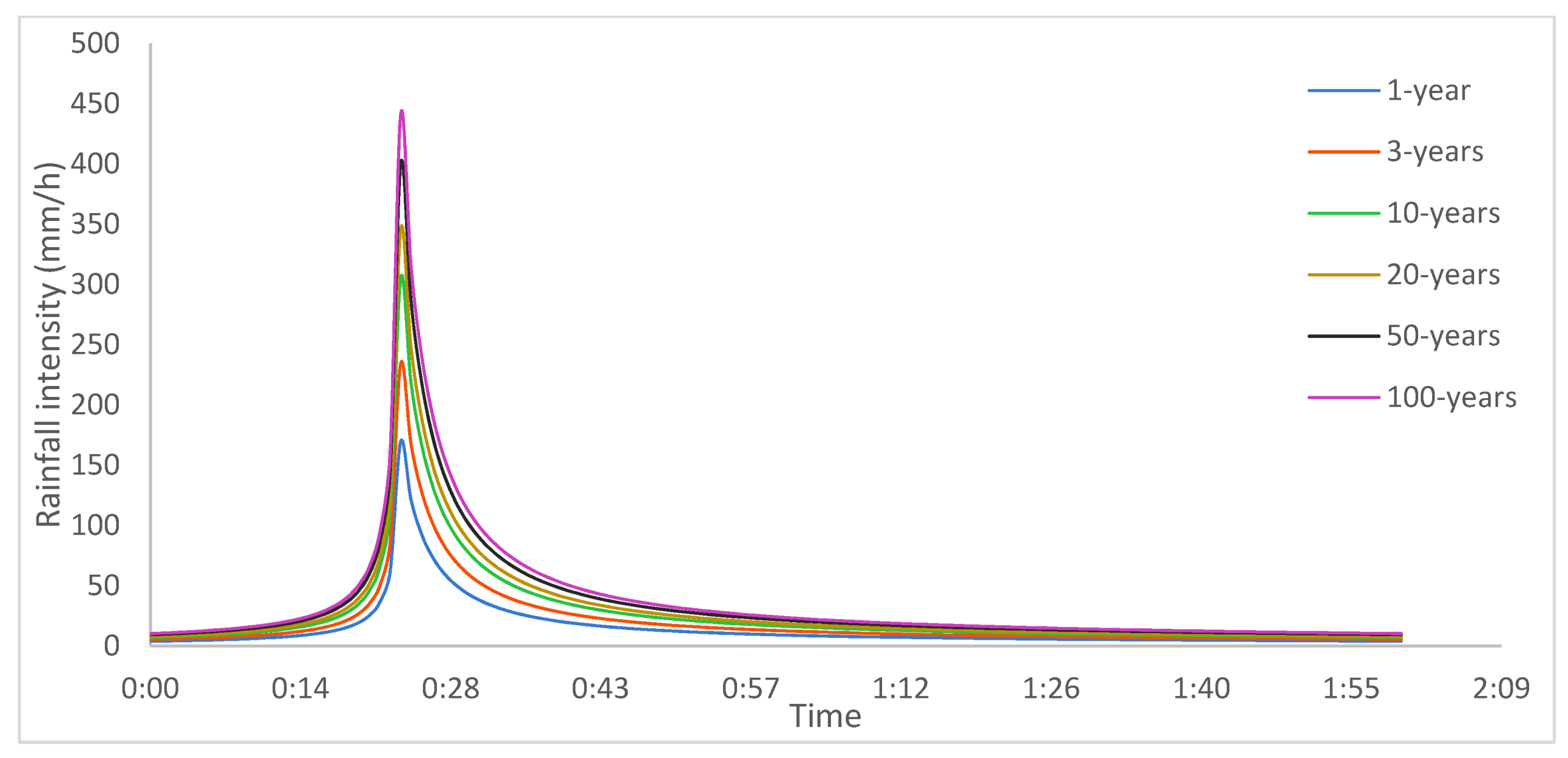
The precipitation data used in this study included the design storms and the historical time series. According to the rain intensity equation developed for Changchun [31] and the ‘Chicago method’ [32], the design storms of 1, 3, 10, 20, 50, and 100 years were derived, respectively, with a rainfall peak coefficient of 0.2 and a rainfall duration of 120 min (Figure 3). The rain intensity equation was derived from the measured data from 1983 to 2012 [31]:

$$q=\frac{2455\left(1+0.71\log P\right)}{{\left(t+10\right)}^{0.816}}$$

(8)

where q is the rainfall intensity (L/hm² -s), P is the design recurrence period (a), and t is the rainfall duration (min).

Three typical water years were picked within the range from 2011 to 2020, which included 2014 (dry year), 2018 (average year), and 2016 (wet year), with a yearly rainfall of 446 mm, 607.3 mm, and 890.8 mm, respectively. The snowmelt simulation was conducted for the period from November 2016 to March 2017 with a total of 65.7 mm of rainfall.

3.3. Model Settings

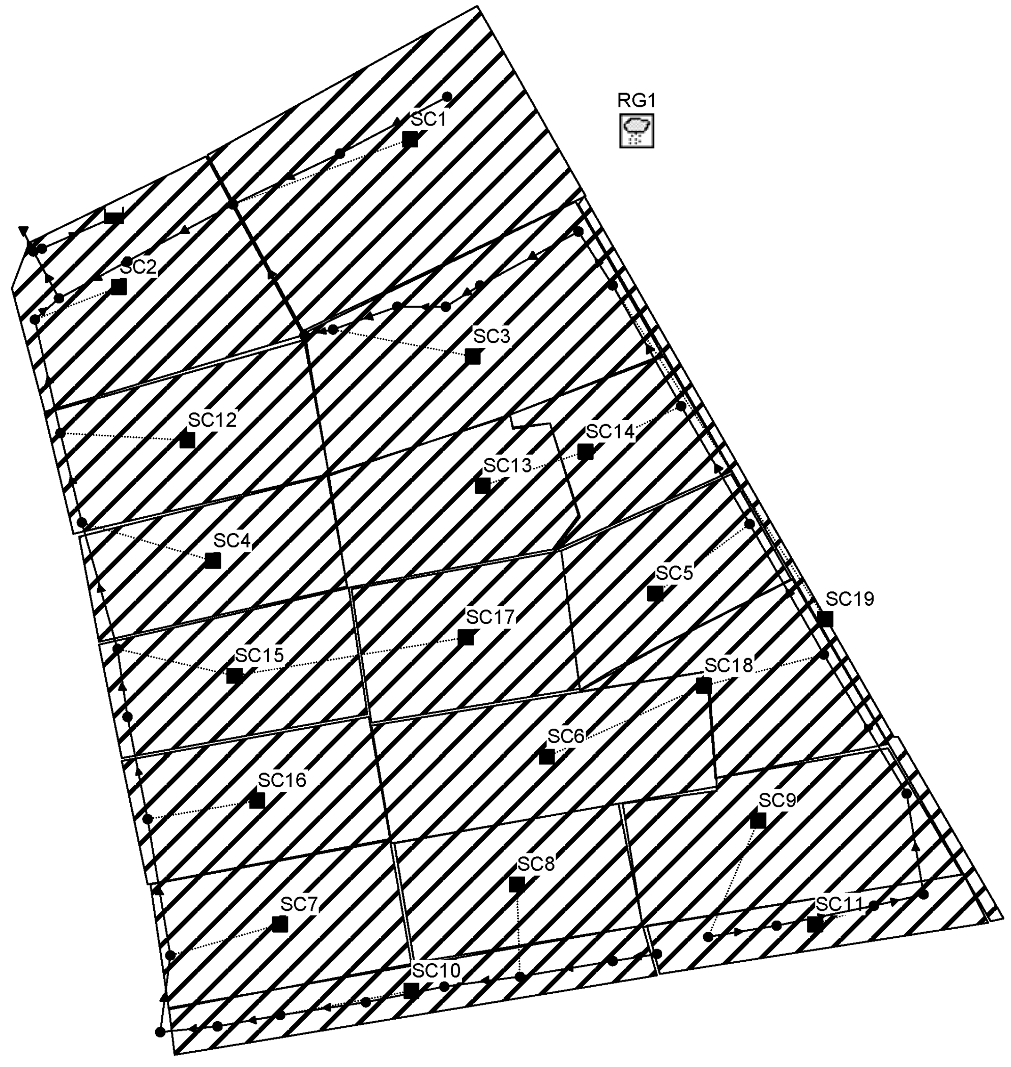
The baseline and LID scenarios were created for the SWMM runs. In the baseline, the study area was generalized into 19 sub-catchments, 36 pipes, 36 nodes, and 1 drainage outlet (Figure 4). On top of the baseline settings, the LID facilities were added into sub-catchments according to the design layouts of the architectural plans in the LID scenario.

While the study area was a community being built and the flow observation was unavailable, the model parameters were calibrated to meet the local drainage design standards (

Table 1. SWMM model hydrological and hydraulic parameter settings.

Parameter Name		Value
Manning n-value Manning n-value	Permeable area	0.05~0.24
	Impermeable area	0.011~0.024
Depression Storage	Permeable area	1.3 mm
Depression Storage	Impermeable area	5 mm
Horton model	Maximum infiltration rate	62 mm/h
Horton model	Minimum infiltration rate	2.5 mm/h
Green–Ampt Model	Suction head	290.068 mm
Green–Ampt Model	Conductivity	2.5 mm/h
Green–Ampt Model	Initial loss	0.108%
Conduit Manning n-value		0.011~0.015

,

Table 2. Parameters of each permeable pavement.

Layer	Parameter	Permeable Concrete Pavers	Permeable Plastic Pavers	Permeable Percolation Plates	Permeable Brick Pavers	Permeable Parking
Surface	Berm Height (mm)	0	0	50	0	20
	Vegetation Volume Fraction	0	0	0	0	0.15
	Surface’s roughness	0.11 *	0.11 *	0.11 *	0.11 *	0.11 *
	Surface Slope (%)	1 *	1 *	1 *	1 *	1 *
Pavement	Thickness (mm)	100	120	182	190	180
	Void radio	0.15 *	0.15 *	0.15 *	0.15 *	0.15 *
	Permeability (mm/h)	100 *	100 *	100 *	100 *	100 *
Storage	Thickness	300	300	300	200	300
	Void radio	0.75 *	0.75 *	0.75 *	0.75 *	0.75 *
	Seepage rate (mm/h)	300	300	300	300	300

Note: The asterisk indicates the model default value.

,

Table 3. Parameters of bio-retention cell and vegetative swale.

Layer	Parameter	Bio-Retention Cell	Vegetative Swale
Surface	Berm Height (mm)	100	200
	Vegetation Volume Fraction	0.15 *	0.10
	Surface’s roughness	0.24	0.24
	Surface Slope (%)	8.56 *	2.50
Soil	Thickness (mm)	400	-
	Porosity	0.44	-
	Field Capacity	0.06	-
	Wilting Point	0.02	-
	Conductivity (mm/h)	210	-
	Conductivity Slope (%)	5	-
	Suction Head	49	-
Storage	Thickness	100	-
	Void radio	0.75 *	-
	Seepage rate (mm/h)	300	-

Note: The asterisk indicates the model default value.

and

Table 4. LID settings in each sub-catchment area.

Sub-Catchment	Areas (m2)	LID-Area (m2)			LID Area Ratio	% Impervious
		Permeable Pavement	Bio-Retention Cell	Vegetative Swale
SC1	4121	1825	372	/	0.53	45
SC2	2675	866	830	/	0.63	37
SC3	3289	315	1028	/	0.41	59
SC4	1854	549	88	/	0.34	52
SC5	1699	221	360	/	0.34	61
SC6	2371	1172	/	/	0.49	33
SC7	1988	426	467	/	0.45	45
SC8	1992	409	279	/	0.35	53
SC9	2710	309	573	/	0.33	55
SC10	1557	1530	/	/	0.98	5
SC11	1128	1010	/	/	0.90	10
SC12	2240	767	648	/	0.63	29
SC13	1893	1123	240	/	0.72	3
SC14	1381	177	967	/	0.83	33
SC15	1923	272	621	/	0.46	47
SC16	2038	1056	368	/	0.70	41
SC17	1938	409	505	/	0.47	46
SC18	1663	342	913	/	0.75	28
SC19	568	212	/	211.83	0.75	5

). The Chinese Ministry of Housing and Urban-Rural Development issued the “Sponge City” Construction Guideline in October 2014, which currently requires the total annual surface runoff control rate to reach 85%, corresponding to a design storm of 26.6 mm in Changchun [33,34]. Both infiltration methods were parameterized to represent the silty clay, which was the soil type of the study area.

The parameters for snowmelt simulation mainly included maximum melting coefficient, minimum melting coefficient, base temperature, and free-water capacity fraction, which were assigned according to the references (

Table 5. Snowmelt parameters.

Parameter Name	Value			References
	Plowable	Impermeable	Permeable
Max. Melt Coefficient (mm/h/°C)	0.000	0.020	0.020	[12]
Min. Melt Coefficient (mm/h/°C)	0.001	0.100	0.150	[12]
Base Temperature (°C)	0	0	0	-
Fraction Free Water Capacity	0.100	0.100	0.100	[13]
Antecedent Temperature Index (ATI)	0.5			User Manual
Negative Melt Ratio	0.6			User Manual

).

3.4. Evaluation Indices

The outputs generated by SWMM were analyzed and summarized by statistics such as surface runoff control rate and runoff coefficient. The surface runoff control rate was calculated by the following equations:

$$Cr=100\%-\frac{P_{out}}{P_{total}}\times 100\%$$

(9)

where Cr is the total runoff control rate (%), P_out is the total outflow precipitation, and P_total is the total precipitation. The runoff coefficient was calculated as follows:

$$\alpha =R/P$$

(10)

where a is the runoff coefficient, R is the depth of runoff (mm), and P is the depth of precipitation (mm).

4. Results and Discussion

4.1. The LID Effect in the Study Area

The LID could effectively regulate the storm runoff in this study. The SWMM model was applied to simulate the baseline and the LID scenario under a series of 2-h design storms with recurrence periods of 1, 3, 10, 20, 50, and 100 years, respectively. The Horton method was used for modeling infiltration in this section. Since the storms generally peaked approximately at 24 min, the simulation time was set to 6 h long. In the baseline, the existing sewer system could guarantee no overflow for a 3-year design storm that meets the local drainage standard. In comparison, no nodal overflow was observed for up to 50-year design storms in the LID scenario.

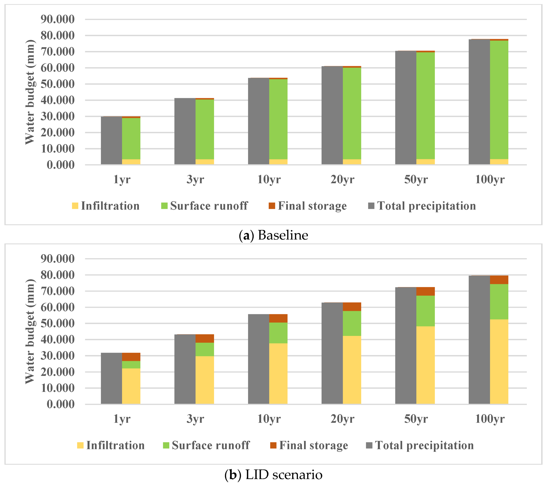
The runoff-reduction effect of LID tended to drop with the increase in the recurrence of the design storms. In the baseline, the surface runoff took approximately 85–94% of the total water budget, while infiltration accounted for 5–12% of the total water budget (Figure 5). The runoff coefficients of the baseline ranged between 0.86 and 0.95 (

Table 6. Runoff reduction rates for various design storms.

Design Storms	Runoff Coefficient		Runoff Reduction Rates
	Baseline	LID
1 year	0.86	0.15	82.32%
3 years	0.90	0.20	77.31%
10 years	0.92	0.24	74.08%
20 years	0.93	0.25	72.71%
50 years	0.94	0.27	71.21%
100 years	0.95	0.28	70.19%

). In the LID scenario, the infiltration volume rose to between 66% and 70% of the water budget, while the ratio of the surface runoff volume dropped to only 15–30%. The runoff coefficients were also significantly reduced to the range of 0.15–0.28. Along with the increase in the recurrence period, the runoff reduction effects of LID tended to fall, though still ranging from 70% to 82% (Table 6).

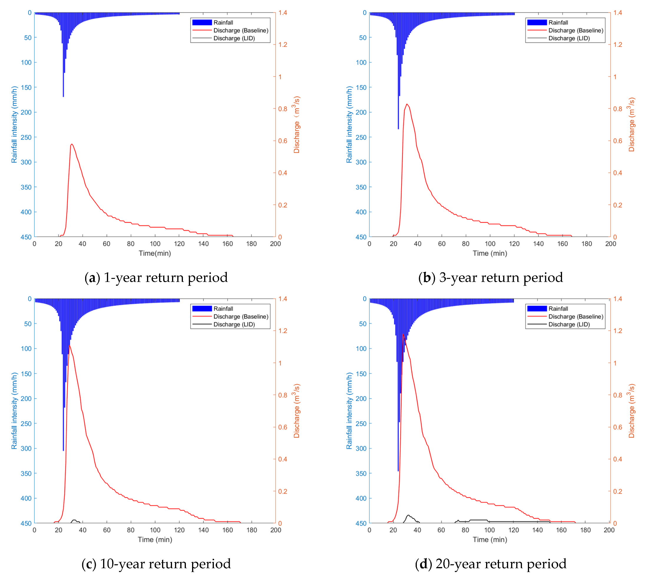
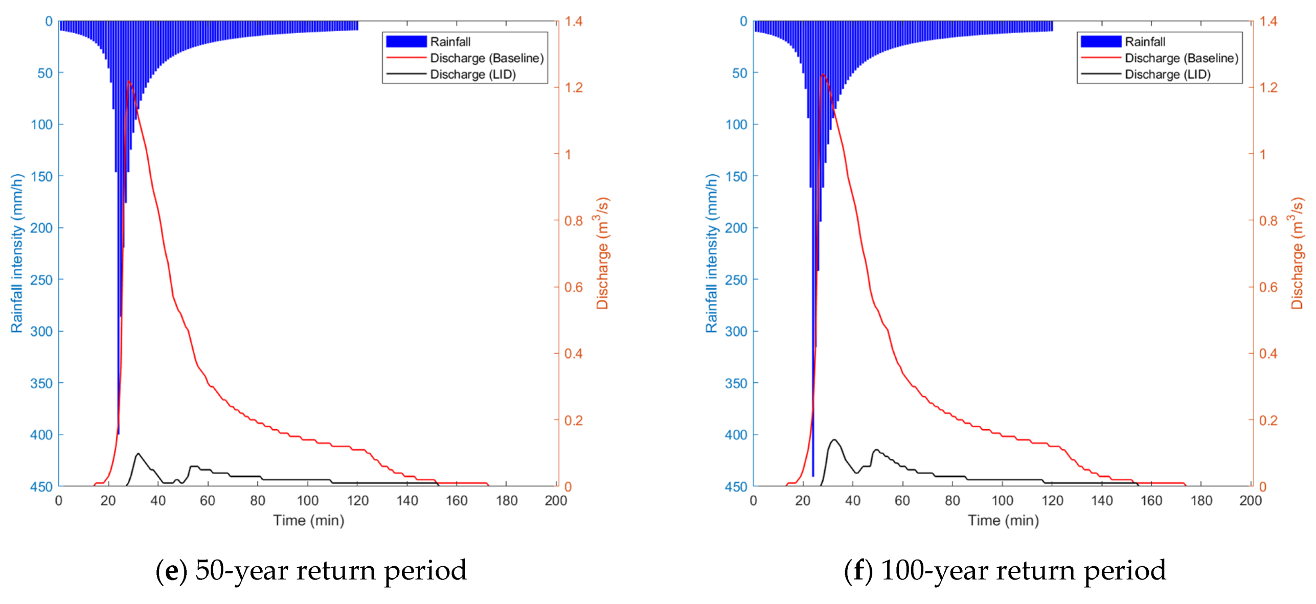
The inverse relationship between the runoff-reduction effect of the LID and the recurrence period could also be shown from the outlet hydrographs. In the baseline, hydrographs of the last conduit of the sewer system indicate that the flood peak closely followed the rain peak with a 4–7 min time lag, and the peak flow increased from 0.58 m³/s to 1.24 m³/s with the recurrence (Figure 6 and

Table 7. Peak flows of the pipe at the outlet.

Recurrence (Years)	Rainfall		Baseline		LID Scenario		Flow Reduction Rates
	Peak Flow (mm/h)	Arrival Time (h:mm)	Peak Flow Rate (m3/s)	Arrival Time (h:mm)	Peak Flow Rate (m3/s)	Arrival Time (h:mm)
1	169.51	0:24	0.58	0:31	0	0:00	100.0%
3	234.22	0:24	0.83	0:31	0.03	1:41	96.4%
10	305.12	0:24	1.11	0:29	0.07	1:06	93.7%
20	345.95	0:24	1.18	0:28	0.1	0:59	91.5%
50	399.91	0:24	1.22	0:28	0.13	0:55	89.5%
100	440.74	0:24	1.24	0:28	0.15	0:51	87.9%

). In the LID scenario, under the condition of a 1-yr storm event, no flow occurred and the flow reduction rate became 100%. Since the 3-year storm event, the flow reduction rates had dropped to 87.9–96.4%, though the peak flow was only 0.03–0.15 m³/s and the peaks appeared 27–77 min later than the rain peaks. It can be inferred that with the increase in rainfall, the effect of runoff reduction turned weaker as the storage of the LID became saturated.

4.2. Comparison of the Infiltration Methods

4.2.1. Design Storms

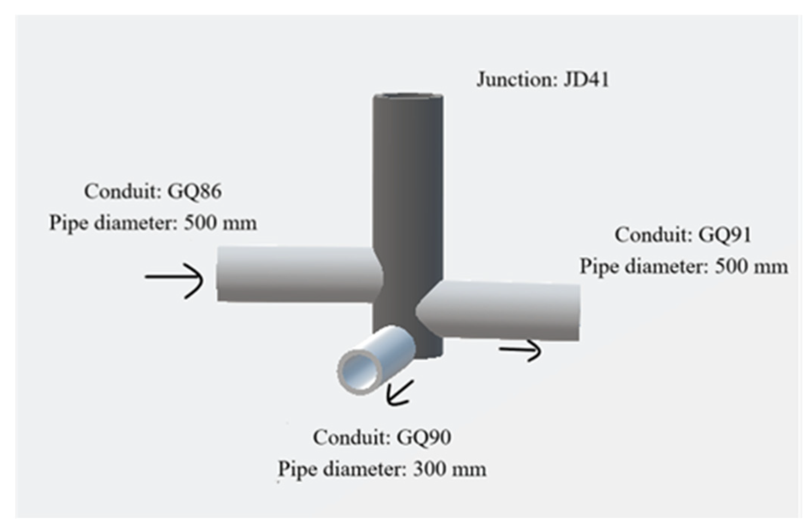
Due to the low percentage of the pervious area of the sub-catchment in the baseline, the selection of the infiltration method appeared to have negligible effect on the outflow discharge (Figure 7). After adding the LID, however, the choice of the infiltration method resulted in slightly different hydrographs. The hydrograph exhibited two peaks with the 100-year design storm setting. The two peaks were due to the presence of a bifurcation above the outlet of the catchment (Figure 8). The upstream 500 mm pipeline was connected to the downstream municipal mainline, while the third pipe on the side with a 300 mm diameter connected at the bottom of the manhole would first lead the flow to a stormwater storage module [35]. So, the first peaks of the hydrographs were mainly contributed by the incoming runoff from the upstream, and the magnitudes between the two infiltration methods were close.

The second peaks were caused by the backwater flow from the storage module after it became saturated, when the peak rate of the Horton method was higher than that of the Green–Ampt method. This might be due to the fact that the Horton method simulated infiltration as a function of time by following a decreasing exponential curve, which appeared to neglect the role of capillary potential gradients during the decline of infiltration capacity over time [36], while the Green–Ampt method used the average suction condition to generalize the substrate potential at the wetting front that may overall reflect a more realistic condition [25,37].

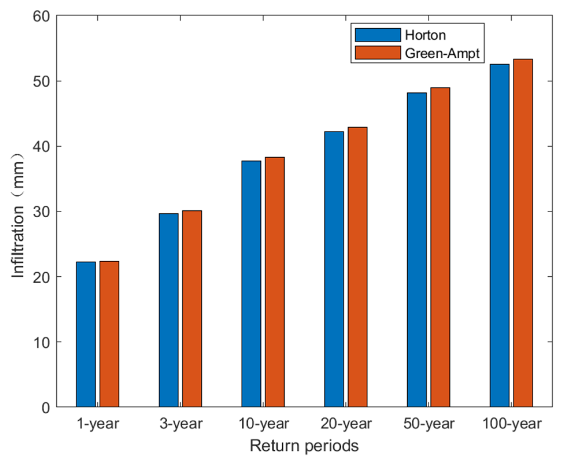
Two infiltration methods led to distinct outflows of the catchment. In the baseline, the peak flow at the outlet reached 0.83 m³/s and 1.2 m³/s for the 3-year and 100-year rainfall, respectively. In the LID scenario, however, no flow was observed during the 3-year storm event; during the 100-year storm event, the peak flow was only 0.15 m³/s, and the outflow volume was 283.5 m³, simulated by the Horton method, which was 17.4% higher than that with the Green–Ampt method. This was because the infiltration depth of the Green–Ampt method was larger than that of the Horton method (Figure 9). Such a difference in the outflow, however, could be hardly revealed simply from the direct comparison between the surface runoff simulated by the two infiltration methods.

As a result, compared to the Green–Ampt method, the Horton method tended to generate lower infiltration, leading to a higher and faster outflow released from the LID. Therefore, in the case of a simulation task driven by a heavy design storm, the Horton method resulted in a lower rate of runoff reduction, which, on the other hand, may serve as a relatively more conservative estimate for the worst-case scenario when designing the drainage system.

4.2.2. Measured Rain Events

The difference caused by the choice of the infiltration methods could also be examined by the observed continuous rain event. The SWMM model was applied to simulate the seasonal runoff for the baseline and the LID scenario (

Table 8. Comparisons of the runoff control rates among the water years.

Year	Rainfall (mm)	Infiltration Methods	Runoff Depth (mm)		Runoff Coefficients
			Baseline	LID Scenario	Baseline	LID Scenario
Dry Year (2014)	446	Horton	202.2	77.5	0.453	0.174
		Green–Ampt	202.0	47.3	0.453	0.106
Average Year (2018)	607.3	Horton	337.0	111	0.555	0.183
		Green–Ampt	336.5	77.2	0.554	0.127
Wet Year (2016)	890.8	Horton	549.2	160.8	0.617	0.181
		Green–Ampt	547.2	121.9	0.614	0.137

), driven by the continuous rain events in 2014 (dry), 2016 (wet), and 2018 (average), respectively. Since the simulation lasted for a full year, evaporation was modeled.

Distinct from the design storms, it appeared that with the observed continuous rain events, the runoff coefficients using the Green–Ampt method were lower than those using the Horton method regardless of the addition of the LID (Table 8), because the Green–Ampt method tended to cause greater infiltration than the Horton method, as stated in the above. After the LID facilities were added, the yearly runoff coefficients with regards to the Horton method were at least 1.3 times higher than those modeled by the Green–Ampt method in any one of the three selected years.

Therefore, despite that the two infiltration methods led to a similar surface runoff forced by the design storms except the 100-year event, a significant difference in the runoff-reduction effect exists driven by the continuous rain events (Table 8). This poses an alarm to the LID designers and drainage engineers that the interchange between the Horton and Green–Ampt methods may lead to a misleadingly negligible difference in surface runoff through the analysis of the design storms, but could lead to a remarkable variance in the hydrologic performance during the long-term, real events, which can be expected to cause more uncertainty in warmer climates with prevalently continuous rain events.

4.3. Seasonal Variations of LID Performance

4.3.1. Seasonal Water Budgets Driven by the Measured Rain Events

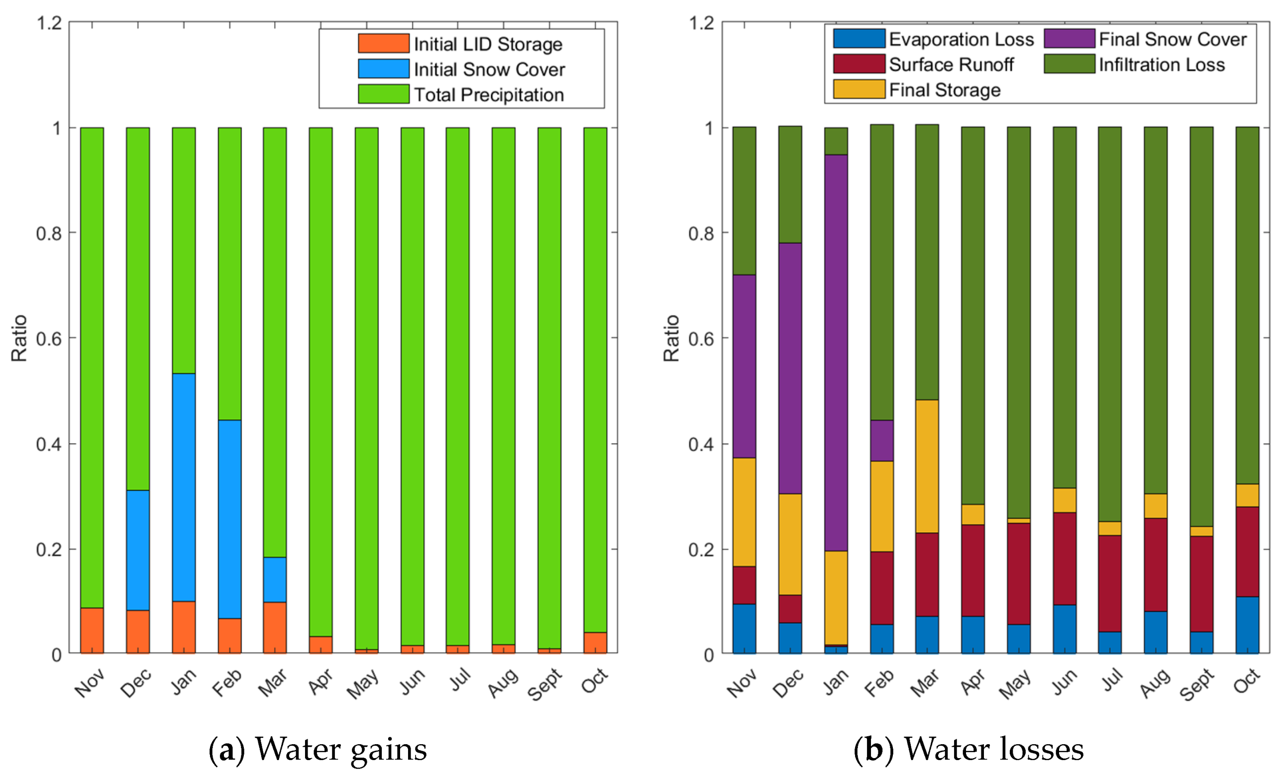
To disentangle the effect of LID on the summer and winter water budgets in the study area, the model was re-run from April 2016 to April 2017 to calculate the monthly water balance (Figure 10). Compared to the relatively stable monthly water budgets in the summer (April–October), the monthly water budgets in the winter (November–March) became complicated due to the varying depths of the snowpack. The snowpack reached its peak in January and almost no surface runoff was formed until February. Then, as the snowpack started to melt, the share of surface runoff in the water budget rapidly increased, along with the reduction in the water storage across the catchment from March to April. This indicates that the LID designers need to consider the freezing and thawing cycles for the applications in the cold regions, which would affect the peak time of the snowmelt runoff.

To better study the effects of snowmelt in a cold climate on urban runoff, the precipitation data from November 2016 to April 2017 were extracted and utilized for separate snowfall simulations. In the baseline, the summer infiltration accounted for 72.7% of the total water loss, and surface runoff took up 18.2% (Figure 10). In the LID scenario, the winter infiltration accounted for 64.3% of the total loss, and surface runoff accounted for 16.7% of the total loss (

Table 9. Water budgets during the winter.

Water Balance	Baseline	LID Scenario
Initial LID water storage (mm)	\	1.91
Total precipitation (mm)	65.70	65.70
Evaporation (mm)	6.60	12.53
Infiltration (mm)	10.11	42.46
Surface runoff (mm)	49.03	11.04
Final water storage (mm)	0.00	1.91

). The lower ratios of infiltration and runoff in the winter indicate that the snow covers created extra storage, which held snowfall from becoming infiltration and runoff. Noticeably, the water budget ratios of the winter were not far from those of the summer, so the LID could effectively manage surface runoff in both winter and summer, possibly owing to the presence of frequent freezing-thawing cycles [38,39].

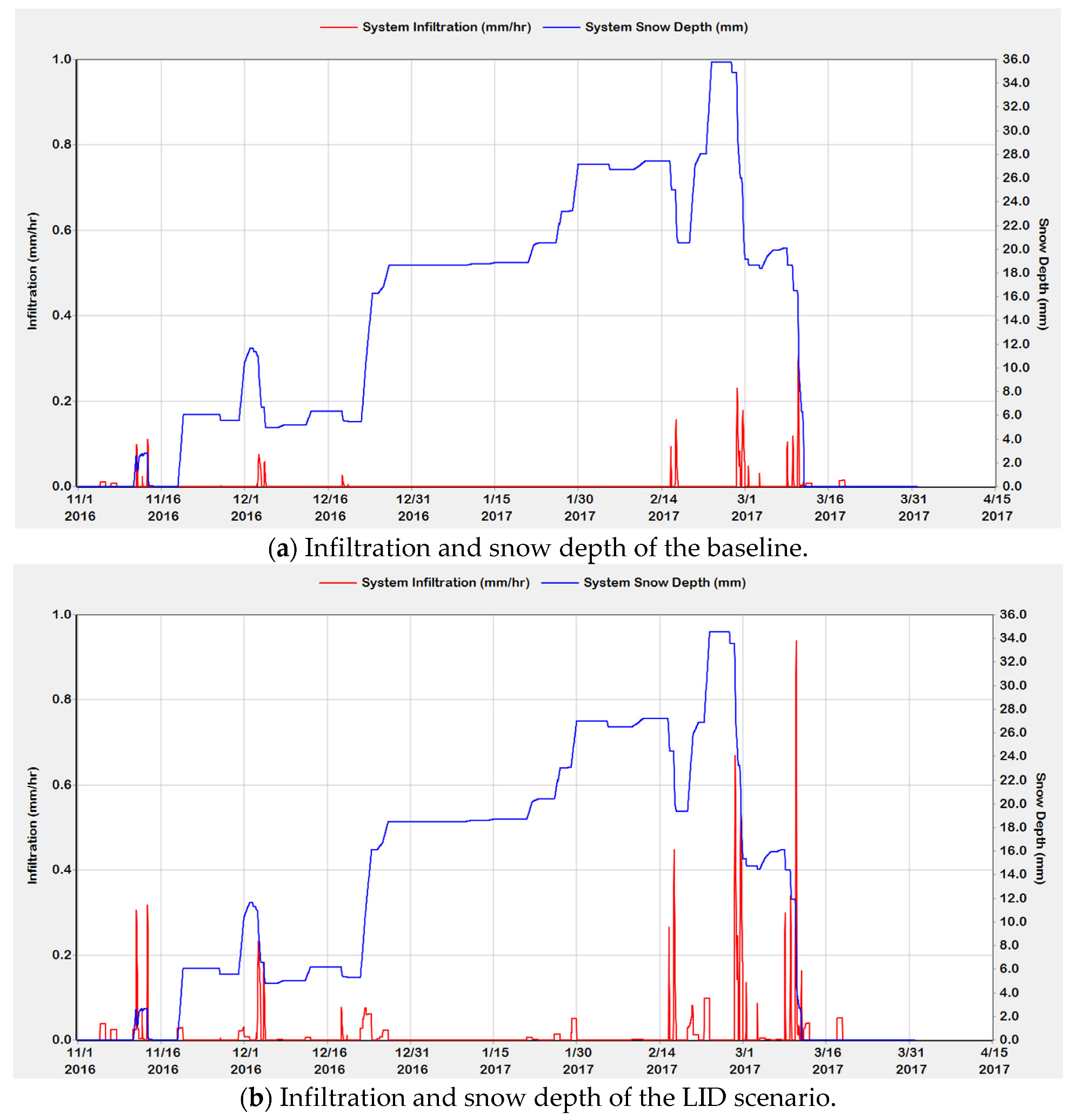
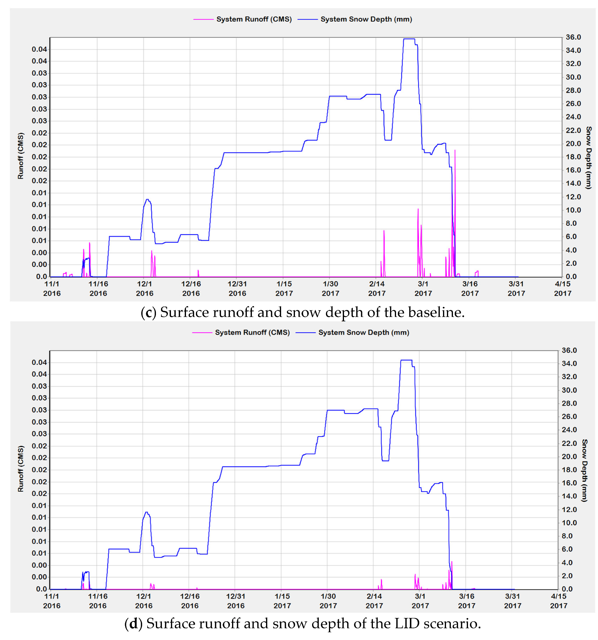
The outflow of the snowmelt runoff from the outlet had a different dynamic from that of the summer rainfall-runoff process. Unlike summer, winter snowfall did not melt immediately to form surface runoff or infiltration, but continued to accumulate at the surface (Figure 11). So, the LID did not provide the immediate regulation of surface runoff in winter like in summer, but resumed functioning in the late winter. However, LID still managed to significantly reduce the peak outflow down to lower than 0.004 m³/s from November 2016 to March 2017. It, therefore, can be argued that the LID contributed to relieving the pressure of the storm drains in the face of the spring runoff, as well as increasing the groundwater recharge for the dry regions [40,41].

4.3.2. Seasonal Runoff-Reduction Effects

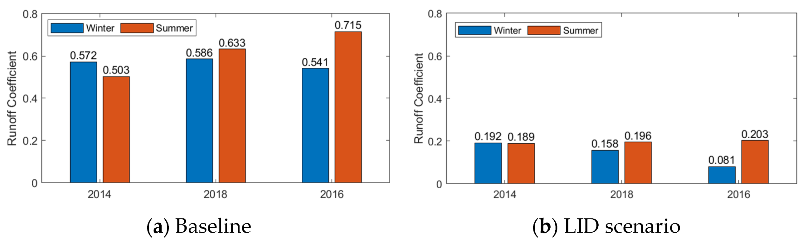
The seasonal runoff coefficients were calculated based on the observed precipitation events (Figure 12). Winter snowfall was 52.3 mm, 53.4 mm, and 47.8 mm in the dry (2014), average (2018), and wet (2016) years, respectively, accounting for 11.7%, 7.9%, and 6% of the total annual precipitation; correspondingly, the winter snowmelt runoff accounted for 11.9%, 7.2%, and 4.5% of the total water budget, respectively. In the LID scenario, the summer runoff coefficient in 2014 was almost equal to that of winter when the summer rainfall was 7.5 times greater than the winter snowfall (

Table 10. Annual precipitation depths.

Year	Precipitation depths (mm)
	Summer	Winter	Total
2014	394.1	52.3	446.4
2018	559.5	47.8	607.3
2016	837.4	53.4	890.8

). Due to the seasonal snow covers with low or zero permeability in winter, the hydrologic performance of LID was compromised and became less effective in reducing runoff than in summer.

Meanwhile, the runoff reduction rate increased with the precipitation in both winter and summer, which was the opposite of the result of the design storms (Figure 12). It can be inferred that with the real rain conditions, the LID facilities were hardly filled up so that the LID had the potential of managing the urban runoff in water-sensitive environments, such as cold areas [42].

5. Conclusions

This work looked into the uncertainty of the two infiltration methods, as well as the seasonal runoff, in affecting the LID performance in the cold climate. The study selected a residential community under construction in Changchun, Jilin Province, China as the study area, and used the SWMM to simulate the baseline and the LID scenario. The following conclusions were drawn through the analyses of a variety of rainfall patterns, infiltration methods, and landscapes.

(1)

In case of the design storms with the return periods of 1, 3, 10, 20, 50, and 100 years, the runoff coefficients of the LID scenario, according to the current design standards, were much smaller than those of the baseline, indicating that the LID facilities could effectively control the runoff generation. However, with the increase in rainfall, the storage capacity of the LID facilities became gradually used up and the runoff reduction rate gradually decreased.

(2)

The Horton and Green–Ampt methods were found to result in different estimations of the LID capacity for managing the surface runoff, especially during the real events. The outflows of the Horton method at the outlet were 17.4% higher than Green–Ampt for the 100-year design storm. It was also found through the measured precipitation time series of the dry, average, and wet years, the annual runoff coefficients with regards to the Horton method were at least 1.3 times higher than those modeled by the Green–Ampt method. This is because compared to the Green–Ampt method, the Horton method tended to generate lower infiltration, leading to a higher and faster outflow from the LID. In case of a simulation task driven by a heavy design storm, the Horton method resulted in a lower runoff reduction rate, which may be a more conservative estimate of the worst-case scenario for designing the drainage system, especially when the input and validation datasets are inadequate. This suggests that the choice of the infiltration method is critical when designing the LIDs by means of simulations.

(3)

Unlike summer, snowfall in winter did not melt immediately to form runoff or infiltration, so the effect of managing the winter runoff by the LID was not directly related to the snowfall intensity, but more to the temperature. The formation of the seasonal snow covers reduced the permeability of LID, undermining the LID capacity for runoff reduction in the winter. However, LID still exhibited an overall decent regulation of winter runoff compared with the baseline, possibly owing to the presence of frequent freezing-thawing cycles.

References

- Yu, H.; Zhao, Y.; Fu, Y.; Li, L. Spatiotemporal Variance Assessment of Urban Rainstorm Waterlogging Affected by Impervious Surface Expansion: A Case Study of Guangzhou, China. Sustainability 2018, 10, 3761. [Google Scholar] [CrossRef] [Green Version]
- Wang, H.; Mei, C.; Liu, J.; Shao, W. A new strategy for integrated urban water management in China: Sponge city. Sci. China Technol. Sci. 2018, 61, 317–329. [Google Scholar] [CrossRef]
- Yin, J.; Ye, M.; Yin, Z.; Xu, S. A review of advances in urban flood risk analysis over China. Stoch. Environ. Res. Risk Assess. 2015, 29, 1063–1070. [Google Scholar] [CrossRef]
- Dai, L.; van Rijswick, H.F.; Driessen, P.P.; Keessen, A.M. Governance of the Sponge City Programme in China with Wuhan as a case study. Int. J. Water Resour. Dev. 2018, 34, 578–596. [Google Scholar] [CrossRef]
- Liu, H.; Jia, Y.; Niu, C. “Sponge city” concept helps solve China’s urban water problems. Environ. Earth Sci. 2017, 76, 473. [Google Scholar] [CrossRef]
- Zaqout, T.; Andradóttir, H.Ó.; Arnalds, Ó. Infiltration capacity in urban areas undergoing frequent snow and freeze–thaw cycles: Implications on sustainable urban drainage systems. J. Hydrol. 2022, 607, 127495. [Google Scholar] [CrossRef]
- Sterpi, D. Effect of freeze–thaw cycles on the hydraulic conductivity of a compacted clayey silt and influence of the compaction energy. Soils Found. 2015, 55, 1326–1332. [Google Scholar] [CrossRef] [Green Version]
- Fouli, Y.; Cade-Menun, B.J.; Cutforth, H.W. Freeze–thaw cycles and soil water content effects on infiltration rate of three Saskatchewan soils. Can. J. Soil Sci. 2013, 93, 485–496. [Google Scholar] [CrossRef]
- Davis, A.P.; Stagge, J.H.; Jamil, E.; Kim, H. Hydraulic performance of grass swales for managing highway runoff. Water Res. 2012, 46, 6775–6786. [Google Scholar] [CrossRef]
- Van Der Kamp, G.; Hayashi, M.; Gallen, D. Comparing the hydrology of grassed and cultivated catchments in the semi-arid Canadian prairies. Hydrol. Process. 2003, 17, 559–575. [Google Scholar] [CrossRef]
- Moghadas, S.; Leonhardt, G.; Marsalek, J.; Viklander, M. Modeling Urban Runoff from Rain-on-Snow Events with the U.S. EPA SWMM Model for Current and Future Climate Scenarios. J. Cold Reg. Eng. 2018, 32, 04017021. [Google Scholar] [CrossRef]
- Valeo, C.; Ho, C.L.I. Modelling urban snowmelt runoff. J. Hydrol. 2004, 299, 237–251. [Google Scholar] [CrossRef]
- Heineman, M.; Bui, F.; Beasley, K. Calibration of urban snow process and water quality model for Logan Airport. In Proceedings of the World Environmental and Water Resources Congress 2010: Challenges of Change, Providence, RI, USA, 16–20 May 2010. [Google Scholar]
- Borris, M.; Österlund, H.; Marsalek, J.; Viklander, M. Snow pollution management in urban areas: An idea whose time has come? Urban Water J. 2021, 18, 840–849. [Google Scholar] [CrossRef]
- Zhicheng, G.; Yuansheng, D. Modeling the hydrological process of drainages in cold regions. J. Glaciol. Geocryol. 2003, 25 (Suppl. S2), 266–272. [Google Scholar]
- Chengshu, W.; Xiaonan, Y.; Wenyi, S.; Xingmin, M.U.; Peng, G.A.O.; Guangju, Z.H.A.O.; Xiaoyan, S.O.N.G. Soil Water Storage Capacity and Rainwater Infiltration in Hilly-Gully Loess Region under Severe Rainstorm. Acta Pedol. Sin. 2020, 57, 296–306. [Google Scholar]
- Yu, J.; Yang, C.; Liu, C.; Song, X.; Hu, S.; Li, F.; Tang, C. Slope runoff study in situ using rainfall simulator in mountainous area of North China. J. Geogr. Sci. 2009, 19, 461–470. [Google Scholar] [CrossRef]
- Mu, W.; Yu, F.; Li, C.; Xie, Y.; Tian, J.; Liu, J.; Zhao, N. Effects of rainfall intensity and slope gradient on runoff and soil moisture content on different growing stages of spring maize. Water 2015, 7, 2990–3008. [Google Scholar] [CrossRef] [Green Version]
- Baiti, H.B.; Bouziane, A.; Ouazar, D.; Hasnaoui, M.D. Storm Water Management Model Sensitivity to infiltration methods and soils impermeability: The Case of Tangier Experimental Basin, Morocco. J. Mater. Environ. Sci. 2017, 8, 3636–3647. [Google Scholar]
- Parnas, F.E.Å.; Abdalla, E.M.H.; Muthanna, T.M. Evaluating three commonly used infiltration methods for permeable surfaces in urban areas using the SWMM and STORM. Hydrol. Res. 2021, 52, 160–175. [Google Scholar] [CrossRef]
- Hashemi, M.; Mahjouri, N.J.W.R.M. Global Sensitivity Analysis-based Design of Low Impact Development Practices for Urban Runoff Management Under Uncertainty. Water Resour. Manag. 2022, 36, 2953–2972. [Google Scholar] [CrossRef]
- Knighton, J.; Lennon, E.; Bastidas, L.; White, E. Stormwater detention system parameter sensitivity and uncertainty analysis using SWMM. J. Hydrol. Eng. 2016, 21, 05016014. [Google Scholar] [CrossRef]
- Chahinian, N.; Moussa, R.; Andrieux, P.; Voltz, M. Comparison of infiltration models to simulate flood events at the field scale. J. Hydrol. 2005, 306, 191–214. [Google Scholar] [CrossRef]
- Van De Genachte, G.; Mallants, D.; Ramos, J.; Deckers, J.A.; Feyen, J. Estimating infiltration parameters from basic soil properties. Hydrol. Process. 1996, 10, 687–701. [Google Scholar] [CrossRef]
- Van Den Putte, A.; Govers, G.; Leys, A.; Langhans, C.; Clymans, W.; Diels, J. Estimating the parameters of the Green—Ampt infiltration equation from rainfall simulation data: Why simpler is better. J. Hydrol. 2013, 476, 332–344. [Google Scholar] [CrossRef]
- Xie, J.; Wu, C.; Li, H.; Chen, G. Study on storm-water management of grassed swales and permeable pavement based on SWMM. Water 2017, 9, 840. [Google Scholar] [CrossRef] [Green Version]
- Luan, Q.; Fu, X.; Song, C.; Wang, H.; Liu, J.; Wang, Y. Runoff Effect Evaluation of LID through SWMM in Typical Mountainous, Low-Lying Urban Areas: A Case Study in China. Water 2017, 9, 439. [Google Scholar] [CrossRef] [Green Version]
- Rossman, L.A. Storm Water Management Model User’s Manual, Version 5.0.; U.S. Environmental Protection Agency: Washington, DC, USA, 2010.
- Rossman, L.A.; Huber, W.C. Storm Water Management Model Reference Manual Volume I—Hydrology (Revised); U.S. EPA Office of Research and Development: Washington, DC, USA, 2016; Volume 104.
- Huber, W.C.; Dickinson, R.E. Storm-Water Management Model, Version 4. Part A: User’s Manual; U.S. Department of Energy Office of Scientific and Technical Information: Oak Ridge, TN, USA, 1988.
- Liu, Z.; Zhang, L.; Yang, Z.; Li, J.; Zhang, B. Derivation of a new generation of stormwater intensity formula for Changchun. China Water Wastewater 2014, 30, 147–150. [Google Scholar]
- Liu, S.; Yang, S.; Lian, Y.; Zheng, D.; Wen, M.; Tu, G.; Shen, B.; Gao, Z.; Wang, D. Time–frequency characteristics of regional climate over northeast China and their relationships with atmospheric circulation patterns. J. Clim. 2010, 23, 4956–4972. [Google Scholar] [CrossRef]
- Li, H.; Ding, L.; Ren, M.; Li, C.; Wang, H. Sponge city construction in China: A survey of the challenges and opportunities. Water 2017, 9, 594. [Google Scholar] [CrossRef] [Green Version]
- Li, Q.; Wang, F.; Yu, Y.; Huang, Z.; Li, M.; Guan, Y. Comprehensive performance evaluation of LID practices for the sponge city construction: A case study in Guangxi, China. J. Environ. Manag. 2019, 231, 10–20. [Google Scholar] [CrossRef]
- Lynn, T.J.; Nachabe, M.H.; Ergas, S.J. SWMM5 unsaturated drainage models for stormwater biofiltration with an internal water storage zone. J. Sustain. Water Built Environ. 2018, 4, 04017018. [Google Scholar] [CrossRef]
- Beven, K.; Robert, E. Horton’s perceptual model of infiltration processes. Hydrol. Process. 2004, 18, 3447–3460. [Google Scholar] [CrossRef]
- Chen, L.; Xiang, L.; Young, M.H.; Yin, J.; Yu, Z.; van Genuchten, M.T. Optimal parameters for the Green-Ampt infiltration model under rainfall conditions. J. Hydrol. Hydromech. 2015, 63, 93–101. [Google Scholar] [CrossRef] [Green Version]
- He, H.; Dyck, M.F.; Si, B.C.; Zhang, T.; Lv, J.; Wang, J. Soil freezing–thawing characteristics and snowmelt infiltration in Cryalfs of Alberta, Canada. Geoderma Reg. 2015, 5, 198–208. [Google Scholar] [CrossRef]
- Zhao, Y.; Huang, M.; Horton, R.; Liu, F.; Peth, S.; Horn, R. Influence of winter grazing on water and heat flow in seasonally frozen soil of Inner Mongolia. Vadose Zone J. 2013, 12, 1–11. [Google Scholar] [CrossRef]
- Jin-Feng, H.; Shuo, L.; Jun, D.; Hao, Q. Simulation of rainfall and snowmelt runoff reduction in a northern city based on combination of green ecological strategies. Chin. J. Appl. Ecol. 2018, 29, 643–650. [Google Scholar]
- Rasmussen, R.; Liu, C.; Ikeda, K.; Gochis, D.; Yates, D.; Chen, F.; Tewari, M.; Barlage, M.; Dudhia, J.; Yu, W.; et al. High-resolution coupled climate runoff simulations of seasonal snowfall over Colorado: A process study of current and warmer climate. J. Clim. 2011, 24, 3015–3048. [Google Scholar] [CrossRef] [Green Version]
- Feng, Y.; Burian, S.; Pomeroy, C. Potential of green infrastructure to restore predevelopment water budget of a semi-arid urban catchment. J. Hydrol. 2016, 542, 744–755. [Google Scholar] [CrossRef]
Figure 1.
Drainage network.
Figure 2.
Land use classification.
Figure 3.
Design storms for Changchun.
Figure 4.
Model layouts.
Figure 5.
The simulated water budgets driven by different design storms in the baseline (a) and LID scenario (b).
Figure 6.
Hydrographs of the conduit at the outlet in the 1-yr (a), 3-yr (b), 10-yr (c), 20-yr (d), 50-yr (e), and 100-yr (f) design storms.
Figure 7.
Hydrographs of the outlet in 3-yr and 100-yr design storms, simulated by the different infiltration methods in the baseline (a) and LID scenario (b).
Figure 8.
The schematic of the bifurcating junction above the outlet.
Figure 9.
The infiltration depths of the LID scenario simulated by the two infiltration methods.
Figure 10.
Monthly water gains (a) and losses (b) in the LID scenario.
Figure 11.
Relationship between the infiltration and snow depth in the baseline (a) and LID scenario (b), and the relationship between the surface runoff and snow depth in the baseline (c) and LID scenario (d).
Figure 12.
Runoff coefficients of the baseline (a) and LID scenario (b).