Arsenate Removal from the Groundwater Employing Maghemite Nanoparticles

Highlights

• As^V removal in synthetic water representing elemental composition equivalent to contam-inated groundwater of Ballia;
• The prepared γ-Fe₂O₃ nanoparticles (MNPs) show efficient capabilities for As^V removal;
• Inter-parametric interactions revealed that adsorption also occurred through the formation of surface complexes;
• Surface complexation modeling (SCMs) shows the involvement of singlet (FeOH^−0.5) and triplet (Fe₃O^−0.5) species in adsorption;
• Weak electrostatic interactions are responsible for the removal process.

Abstract

An investigation of the potential of γ-Fe₂O₃ (maghemite) nanoparticles (MNPs) to remove As^V from groundwater is reported. The MNPs were synthesized using a modified co-precipitation method via refluxing. The morphological and surface characteristics of MNPs were analyzed using XRD, FTIR, SEM, TEM, and Zetasizer techniques. Their As^V removal potential was explored in synthetic water representing the elemental composition equivalent to arsenic-contaminated groundwater of the Ballia district, Uttar Pradesh, India. The arsenic concentration in the samples collected from the study area was observed to be much more than the provisional WHO guideline value for drinking water (10 µg L⁻¹). An orthogonal array L₂₇ (3¹³) of the Taguchi design of experimental methodology was employed to design the experiments and optimization of As^V removal. The ANN tool was trained to evaluate Taguchi’s outcomes using MATLAB. The percentage of ionic species distribution and surface complexation modeling was performed using Visual MINTEQ. The study explored the effects of pH, temperature, contact time, adsorbent dose, total dissolved solids, and shaking speed on the removal process. The adsorption was found to occur through electrostatic interactions. The inter-parametric analysis demonstrated the involvement of secondary sites affecting the adsorption. The charge distribution multi-sites complexation (CD-MUSIC) model and 2pk-Three-Plane-Model (TPM) indicated the involvement of the reactivity of singlet (FeOH^−0.5) and triplet (Fe₃O^−0.5) species in the examined pH range. The developed nanoparticles are observed to be efficient in As^V removal. This information could benefit field-scale arsenic removal units.

1. Introduction

Arsenic is a toxic, bio-accumulating, redox- and pH-sensitive element. Millions have been exposed to this life-threatening groundwater contaminant over the last few decades [1]. The high mobility of arsenic in aquifer systems is of concern. Trace arsenic toxicity and biomagnification mainly depend on its oxidation state [2]. Arsenic is found in the earth’s crust, from which it leaches into groundwater [3]. Even at low concentrations, its long-term consumption can develop cancers of the lungs, liver, bladder, and kidneys [4]. Countries such as Argentina [5], Bangladesh [6], Brazil [7], Canada [8], Cambodia [9], Chile [10], Ghana [11], Hungary [12], Mexico [13], Pakistan [14], Republic of China, Taiwan, United States of America and Vietnam [14] are affected with arsenic-contaminated groundwater. In India, the states of Assam [15], Bihar [16], Chhattisgarh [17], Himachal Pradesh [18], Jharkhand [19], Punjab [20], Manipur [21], Uttar Pradesh [22], and West Bengal [23] are all reported to have elevated levels of arsenic in groundwater [24,25]. The World Health Organization (WHO) provisional guide value and the Bureau of Indian Standard (BIS) regulatory value 10 µg L⁻¹ in drinking water are set to combat the problems occurring to human health [26,27].

Oxidation and filtration [28], co-precipitation, sedimentation and filtration [29], ion exchange resins [30], adsorption [31], reverse [32], forward osmosis [33], and electrodialysis [34] are all reported techniques for arsenic removal from aqueous solution. Adsorption-based treatments have gained considerable attention due to its large-scale feasibility and easy operation [35]. Moreover, nanotechnology-based water treatment systems offer a logical choice considering their large-scale applicability, resource, and energy efficiency. Therefore, several inorganic nano adsorbents, specifically the oxides of iron [36,37,38], titanium [34,39], aluminum [40,41], copper [42], zinc [43,44], zirconium [45,46] and cerium [47,48], have been reported in relation to arsenic removal. Nevertheless, iron-based nanoparticles are explored largely due to their easy availability, bio-friendly characteristics, intrinsic affinity, and arsenic selectivity [49,50]. Compounds such as nZVI, hematite [51], goethite [52,53], akaganeite [54], and magnetite [37,51,55,56,57] have been extensively explored for As^V removal. However, nanoparticles (NPs) of γ-Fe₂O₃ (maghemite), which is a widely occurring iron oxide [58], still need to be explored widely.

Arsenic removal using nanoadsorbents was reported to occur through several mechanisms. It includes ligand exchange [59], complex coordination [60], chemisorption [61], bidentate-binuclear complexes [62], inner-sphere complexes [63], anion exchange [64], and electrostatic interaction [65,66]. These studies explore the mechanism through batch experiments containing single species (i.e., arsenic) in the aqueous solution [67]. Although, several ions in natural groundwater conditions might affect the removal efficiency and mechanism during adsorption. Understanding the impact of these co-ions on arsenic removal in terms of efficiency and adsorption behavior is necessary. Therefore, this study investigates the arsenic removal characteristics of MNPs in synthetic water having elemental compositions equivalent to real-world groundwater.

Shared charge theory can demonstrate the selective adsorption of different oxyanions onto metallic nano adsorbents [68]. It considers that deprotonated oxygen atoms of ionic species interact with the surface moieties of metal-bearing nano adsorbents, which necessitates exploring the influence of anionic species on the adsorption. Although, the literature investigates the effects of Cl⁻, SO₄², NO₃⁻, and PO₄³⁻ ions on arsenic removal using MNPs [69]. However, the studies evaluating the arsenic sequestration potential of MNPs in groundwater compositions representing typical real-world aquifers are lacking.

The relative concentrations of the dominant inorganic arsenic species (As^III and As^V) vary in natural waters. pH and redox potential (E_h) are the primary factors for arsenic speciation in groundwater [70]. In a highly oxidizing environment (E_h: 600 to 1200 mV), HAsO₄²⁻ and H₂AsO₄⁻ are the dominant arsenic species in the pH range of 2.0–6.5 and 6.5–11.5, respectively. However, low oxidizing (E_h: 0 to 600 mV) and anaerobic environments (E_h: 0 to −800 mV) favor the presence of the uncharged H₃AsO₃species in natural water [71]. Studies exploring the possible interactions of arsenic species with other ions during treatment processes using nanoparticles are needed.

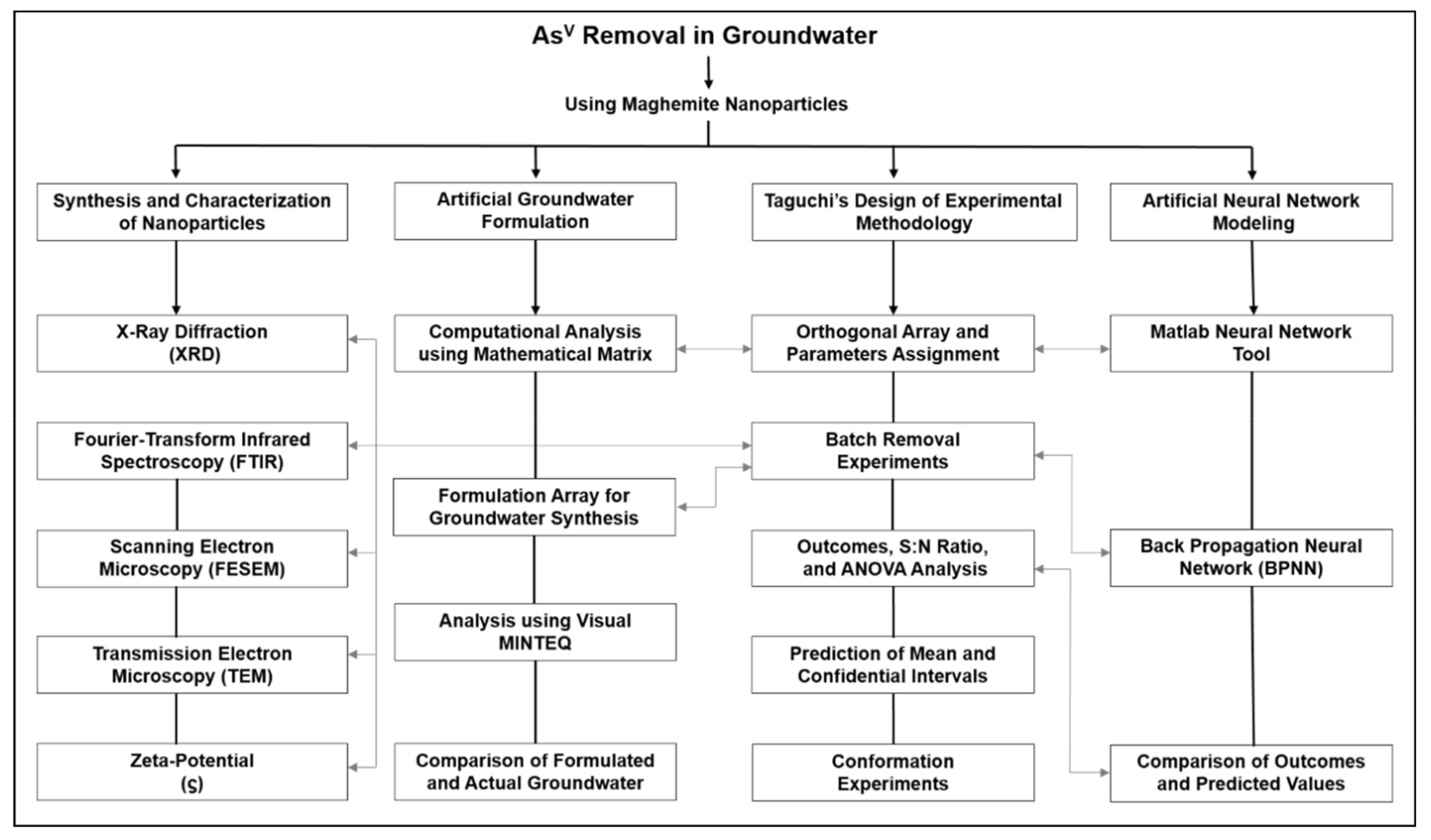
Analyzing interactions among the experimental variables and result outcomes is impractical through one-way classification procedures [72,73] because it requires many experimental runs. Additionally, these explain only the effects of design factors on the average result level. Nevertheless, the experimental design based on mathematical models is relevant and helps to assess the statistical significance of different factors [74,75]. These effectively investigate the effect of multiple factors and potential interactions among the factors through minimum numbers of experimental runs. Therefore, we opted to use Taguchi’s experimental methodology in the present study. Previously, several authors explored the response surface methodology (RSM) to optimize the removal of contaminants, such as fluoride [76], heavy metals [77], and anionic dye [78] using MNPs. However, Taguchi’s optimization methodology has not been reported for As^V removal using these nanoparticles in the literature. Taguchi’s design also considers the study of variations, which is more critical than just the average considered in RSM [79]. It also investigates different parameters affecting process performance characteristics. A brief outline of the components explored in this study is presented in Figure 1.

The present study aims to evaluate the adsorption potential of MNPs for As^V removal using real-world groundwater compositions. It is expected to provide a systematic understanding of the nano adsorbent behavior to research communities on a common platform that develops efficient remediation systems in arsenic-affected areas. Taguchi’s experimental methodology was adopted to maximize the response characteristics by optimizing different process parameters to simultaneously maximize removal percentage at a minimal adsorbent dose and near-neutral pH conditions. Synthetic water with a concentration of constituents similar to actual groundwater composition was used in the experimental runs. The formation of possible competing ion species under six different conditions, such as pH and variable concentration range were identified using Visual MINTEQ, which further explored understanding their effects on As^V adsorption. Finally, the artificial neural network ANN model was trained to evaluate Taguchi’s outcomes using MATLAB. The present results could serve the scientific community by providing a basis for investigating arsenic removal using nanoparticles in groundwater, representing real field-scale applications.

2. Experimental Procedure

2.1. Materials and Reagents

Analytical reagent grade salts FeCl₃·6H₂O (M.W. = 270.3 g mol⁻¹) and FeSO₄·7H₂O (M.W. = 278.01 g mol⁻¹) were purchased from Thermo Fisher Scientific enterprises (Waltham, MA, USA) and utilized as a source of Fe³ and Fe²⁺ ions, respectively, during the synthesis of nanoparticles. The Na₂HAsO₄·7H₂O (M.W. = 312.01 g mol⁻¹) salt, purchased from Merck Enterprises, was used to prepare the arsenic working solution. Analytical grade (ACS) ammonium hydroxide (NH₄OH, 28% w/w), hydrochloric acid (HCl, 37% w/w), perchloric acid (HClO₄, 37% w/w), and sodium hydroxide (NaOH, ≥97%, pellets) were obtained from Sigma-Aldrich (St. Louis, MO, USA). ICP-MS grade (Merck enterprises) standard solutions of cations, anions, heavy metals, and arsenate were used during the calibration. Salts were used to formulate artificial water, according to Table S1. All solutions were prepared in deionized water (Millipore, electrical conductivity, 18.2 MΩ-cm at 25 °C).

2.2. Instrumentations and Equipment

X-ray diffraction (XRD) patterns were performed on a Bruker X-ray diffractometer (Model: D8-Advance, Source: 2.2 kW Cu anode). Infrared (IR) spectra were recorded in the mid-IR range using an Agilent Cary 630 Fourier Transform Infrared spectrometer (Spectral range: 4000–400 cm⁻¹, Sample interface: Diamond ATR). Morphological analysis was undertaken using a Field-Emission Scanning Electron Microscope (Model: Carl Zeiss Ultra Plus) equipped with an In-Lens Detector for surface structure analysis. The high-resolution imaging of nanoparticles was performed through a Field-Emission Scanning Electron Microscope (Model: FE-SEM QUANTA 200 FEG, Gun type: FEG with Schottky emitter) and High-Resolution Transmission Electron Microscope (Model: FEI Tecnai G² 20 S-Twin, Electron source: LaB₆ or W emitter) (FEI Electron Optics International BV Enterprises, Netherlands). The surface charge (ϛ-potential) was measured on a Malvern Zetasizer Nano ZS90 (Light source: He−Ne laser 633 nm, Measurement range: 0.3 nm–100 µm). The concentration of cations (Ca²⁺, Mg²⁺, Na⁺, K⁺) and anions (F⁻, Cl⁻, SO₄²⁻, NO₃⁻) were determined by Ion chromatography (Metrohm, 819-IC-Detector) by employing ion-exchange columns Metrosep-C2-250 and Metrosep-A-Supp-5, respectively. Sulfate and phosphate ion concentrations were determined using a double beam UV-visible spectrophotometer (Agilent Cary 100, Monochromator: Czerny-Turner 0.278 m). Heavy metals were determined by Inductively Coupled Plasma Mass Spectrometry (ICP-MS) (ELAN DRC-e, Perkin Elmer. The metalloid arsenic concentrations were measured using Microwave-Plasma Atomic Emission Spectroscopy (MP-AES) (4100, Agilent Technologies, Santa Clara, CA, USA). The operational parameters utilized for these analyses are detailed in the Supplementary Information (Text S1–S3). The orbital shaking incubator (Model: CIS–24 Plus) from REMI Laboratory Instruments, equipped with a temperature and shaking speed range of 5–60 ± 0.5 °C and 20–250 RPM, respectively, was used to carry out the batch experiments. All the samples were dried in a vacuum oven (Model: LVO 2030) from Daihan Labtech. India Private Limited (Gurugram, New Delhi, India) provided a temperature and vacuum control range of 5–250 ±1 °C and 10–760 mm Hg, respectively.

2.3. Synthesis of Nanostructured Maghemite

The MNPs were developed using a previously reported co-precipitation method [80], with a slight modification by refluxing the Fe²⁺ (ferrous) and Fe³⁺ (ferric) salts. First, 4.2 g of FeSO₄·7H₂O and 3.7 g of FeCl₃ were dissolved in 100 mL of ultra-pure water and poured into a twin round bottom flask. Then, the solution was heated to 90 °C. Afterward, 10 mL of NH₄OH (25%) was added dropwise. The solution was refluxed at a temperature above 90 °C for approximately 45 min and eventually cooled to room temperature. The magnetic precipitates were isolated from the alkaline solution using laboratory magnets and washed to remove all the unwanted non-magnetic and soluble products. Finally, the collected black powders were dried in an anaerobic environment (vacuum oven) for several hours at 60 °C and stored at room temperature. Then, the obtained powdered sample was employed for electronic characterization and adsorption experiments.

2.4. Sample Collection and Analysis

The arsenic sequestration potential of MNPs was examined for real-world water conditions. For this, two samples were collected from near Lohapatti (Location I) and Kanspur (Location II) from the arsenic-affected of district Ballia, Uttar-Pradesh, India (Figure 2). These sample locations represent shallow (Mark II hand-pumps, depth 30–33 m) and deep (Bore-well, depth 66–75 m) aquifer systems. The hand pump and bore-well shaft water were purged for 10–15 min before sample collection. The three samples from each location were collected in pre-washed polyethylene bottles of 500 mL capacity.

One set of sample bottles containing no preservatives was utilized to determine significant cations and anions. The other sets of sample bottles were preserved) with nitric acid (68% w/w) and hydrochloric acid (37% w/w) (1 mL in 500 mL) to determine heavy metals such as iron, manganese, copper, lead, cadmium, zinc, and the metalloid arsenic. After sampling, all the samples were stored at a temperature of ≤4 °C using ice/cold packs or a refrigerator. The pH, electrical conductivity, and total dissolved solids were determined in-situ using a portable analysis kit (HACH, Model: multi HQ 40d, Loveland, CO, USA).

Before sample analysis, all samples were filtered (Whatman^TM 42 1442-125, pore size 2.5 µm). Samples for heavy metals analysis (Fe²⁺, Mn²⁺, Cu²⁺, Pb²⁺, Cd²⁺, Zn²⁺) were further digested in concentrated HNO₃. The minimum detection limit of arsenic by MP-AES was 1.0 µg L⁻¹. The methods related to water samples collection, mode of preservation, and sample preparation for different analyses were followed as stated in the standard procedure(s) [81,82].

2.5. Formulation of Synthetic Water

This study utilized a convenient approach to formulating synthetic water in the workplace. Batch experiments are often not feasible at a laboratory scale using actual groundwater due to large sample volume requirements and temporal variability in groundwater compositions. The approach involved (i) preparation of a matrix matching the required elemental components to the compositions of starting materials (Table S1); (ii) multiplying the inverse matrix with the target concentrations to determine the amount of each starting material to use [80]. Arsenic concentrations were achieved separately from this approach because of the large difference in the magnitude of the concentration of arsenic compared to the other solutes. The calculated and measured compositions of the synthetic waters for locations I and II are shown in

Table 1. Comparison of ionic concentrations between actual groundwater and artificial formulated water.

	Location I				Location II
Element	Actual Groundwater Conc. (mg L−1)	Calculated Values from the Matrix	Measured Synthetic Water Conc. (mg L−1)	Diff. (%)	Actual Groundwater Conc. (mg L−1)	Calculated Values from the Matrix	Artificial Water Conc. (mg L−1)	Diff. (%)
TDS (gravimetric)	435.9	-	411.5	5.6	1590.6	-	1405.7	11.6
TDS (calculated by ions)	337.4	261.4	310.6	7.9	1446	1171.1	1321.5	8.6
Chloride	132	67.1	112.0	15.2	435	222.7	346	20.5
Sodium	33	23.1	28.0	15.2	169	111.2	141	16.6
Bicarbonate	27	27.0	28.0	−3.7	115	114.8	113	1.7
Potassium	15	13.8	13.3	11.3	95	91.6	93	2.1
Fluoride	1.5	1.5	1.5	1.3	3	2.94	3.16	−5.3
Nitrate	20	20.0	21.2	−6.0	140	139.8	139	0.7
Calcium	29	28.9	26.4	9.0	185	185.3	181.5	1.9
Zinc	2	1.9	1.9	5.0	4	4.43	4.1	−2.5
Magnesium	27	27.0	24.5	9.3	33	33.2	32.4	1.8
Sulfate	30	30.1	32.4	−8.0	220	219.4	221.1	−0.5
Silica	18	18.1	18.6	−3.3	42	41.4	42.3	−0.7
Manganese	2	1.9	1.9	7.5	3	3.4	3.2	−6.7
Phosphates	0.91	1.1	1.0	−6.6	2	1.06	1.75	12.5
Arsenate *	0.055	-	0.057	−3.6	0.2	-	0.201	−0.5

* The high difference (%) in calcium and magnesium ions concentration contributes to the high hygroscopic nature of their salts. Similar, the higher variation for sodium ions is due to ignorance of sodium arsenate salts during matrix calculation.

. These synthetic waters were then used for the subsequent batch adsorption experiments for As^V removal.

2.6. Taguchi’s Design of Experimental Methodology

A Taguchi design methodology was used to design the batch adsorption experiments. Orthogonal arrays (OA’s), S:N analysis and variance were used as practical tools to analyze design outcomes [83]. As adopted in the present study, Taguchi’s approach involved four phases: selection of parameters; experimental investigation; analysis; and validation.

2.6.1. Design of Experiment (Phase 1)

The first step in Phase I was selecting for optimization the different factors that can affect the removal of As^V from an aqueous solution. Temperature, pH, dose, and contact time can affect the efficiency of removal of As^V onto the surface of iron^(III) metallic oxide NPs [38,84,85]. Preliminary experiments showed that removal capacity was also affected by total dissolved solids (TDS) and shaking speed cf. Goswami et al. [86] examined the shaking speed’s effect in removing arsenic using copper oxide nanoparticles. Therefore, the parametric design (

Table 2. Process parameters for As^V adsorption onto MNPs nanoparticles in multicomponent ionic systems using Taguchi’s orthogonal arrays (OA’s) design.

	Parameters	Level 1	Level 2	Level 3
A	Arsenate concentration (µg L−1)	55	128	200
B	TDS (mg L−1)	436	1014	1591
C	Shaking speed (rpm)	100	170	240
D	Temperature (°C)	10	20	30
E	pH (pH unit)	7	8	9
F	Dose (g L−1)	0.05	0.10	0.15
G	Contact time (min)	2	53	104

) investigated the effect of seven factors through batch removal studies. Three two-parameter interactions (A.B, A.C, B.C) were also considered for inter-parametric investigations.

2.6.2. Orthogonal Array (OA) and Assignment of Parameters

The second step in Phase I was to design the experimental matrix that defines the data analysis procedure. An appropriate orthogonal array was selected for the controlling parameters suitable for the present study. In selecting a suitable OA, the design must satisfy the following prerequisite:

• Total DOF required for experiment ≤ total DOF of OA.

In this study, the calculated degree of freedom (DOF) is 26 [=no. of parameters (7) × {no. of levels (3) − 1} + {no. of two-parametric interactions (3) × no. of parametric interactions (2) × no. of columns assigned for each interactions (2)}]. Hence, a standard three-level OA of L₂₇ (3¹³) (27—represents the total no. of experimental numbers; 3—parameter levels; 13—represents columns of the experimental layout used to assign test factors and interaction studies) was selected for further study. The details of the reactive surface species and L₂₇ array are shown in Table 3 and Table 4, respectively.

2.6.3. Batch Removal Experiments (Phase 2)

Batch adsorption studies were explored to remove As^V using MNPs for the selected 27 experimental trials having seven process factors with three levels (Table 3). The results were obtained from individual sets in terms of the total amount (q_e) of As^V adsorbed (µg L⁻¹) onto the surface of nanoparticles, as shown in Table 4. Each set of experimental trials was performed in three replications and designated as R₁, R_2, and R₃.

In each experimental trial, 100 mL of an aqueous solution containing different As^V concentrations (levels) were placed in a 200 mL glass stoppered conical flask containing a specific dose of MNPs. The pH was adjusted before each batch experiment using NaOH (0.001 N) and per-chloric acid (0.001 N) without further pH adjustment during the sorption process. Finally, the samples were filtered after the appropriate contact time of the sorption process, and filtrates were analyzed to determine the residual concentration of As^V ions.

The removal capacity $q_e$ (µg mg⁻¹) of As^V from the aqueous solution was calculated by using the following equation:

$${\mathrm{q}}_{\mathrm{e}}={\displaystyle \sum }_{\mathrm{i}=1}^3\frac{({\mathrm{C}}_0-{\mathrm{C}}_{\mathrm{f}})}{\mathrm{W}}$$

(1)

where C₀ and C_f are the initial and final concentration (µg L⁻¹) of As^V, respectively, and W is the adsorbent dose (mg L⁻¹).

2.6.4. Evaluation of Outputs and Performance Assessment (Phase 3)

The explored experimental data was organized with higher-is-better quality characteristics (i) to identify the optimum removal conditions, (ii) along with the potential of an individual factor affecting the adsorption process, and (iii) to estimate the performance (q_e) under optimized conditions. This methodology defines the loss function as a quantity directly related to the deviation from nominal quality attributes. Taguchi identified a quadratic relationship as a practical, viable function that depends on the Taylor Expansion Series, expressed as Equation (2):

$${\mathrm{L}}_{\left(\mathrm{y}\right)}= \mathrm{k} {\left(\mathrm{y}-{\mathrm{m}}_{\mathrm{T}}\right)}^2$$

(2)

where L, k, y, and m denote the loss in removal capacity, proportionality constant (depend on the magnitude of characteristic and removal capacity unit), the experimental value calculated for individual trial, and a target value, respectively. However, Taguchi modifies the loss function into a statistical tool known as the signal-to-noise (S:N) ratio, which is explored further.

2.6.5. Signal to Noise Ratio (S/N)

This attribute of the methodology combines the two characteristics of a distribution into a single metric. The high value of the S:N ratio signifies that the signal is higher than the noise component’s random effects and depicts the optimum value of removal characteristics MNPs. The Signal to noise ratio, S:N, was calculated from replicate experiments according to Equation (3):

$${\left(\mathrm{S}:\mathrm{N}\right)}_{\mathrm{LB}}=-10 \log \frac{{{\displaystyle \sum }}_{\mathrm{i}=3}^{\mathrm{N}}\raisebox{1ex}{$1$}\!\left/ \!\raisebox{-1ex}{${({\mathrm{q}}_{\mathrm{i}})}^2$}\right.}{\mathrm{N}}$$

(3)

where ‘q_i’ is the value of the experimental outcome (adsorption capacity) in an observation, ‘N’ represent the replication number of experiments.

However, Taguchi suggested several methods for analyzing S:N data [87]. Among those, plotting of response curves (average value), ANOVA for raw, and S:N data concerning adsorption capacity for process parameters were examined in the present investigation.

In these factors, the curve plot at the individual level indicates a trend, a pictorial representation showing the effect of parameters on response. The S:N ratio is an experimental response to measure a trial’s variations. Further, the ANOVA test was conducted for the calculated values of adsorption capacity (q_e) and S:N ratio to identify significant parameters such as mean and variance.

2.6.6. Prediction of Average Adsorption Capacity

This section estimates an average adsorption capacity (µ) value at the optimized conditions. The adsorption capacity (µ) for the optimized conditions was estimated using the following equation as suggested by Taguchi:

$${\mathsf{\mu }}_{\mathrm{MNPs} }=\overline{\mathrm{T}}+\left({\overline{\mathrm{B}}}_3-\overline{\mathrm{T}}\right)+\left({\overline{\mathrm{C}}}_2-\overline{\mathrm{T}}\right)={\overline{\mathrm{B}}}_3+{\overline{\mathrm{C}}}_2-\overline{\mathrm{T}}$$

(4)

where $\overline{T}$ represents the value of overall experimental average adsorption capacity, ${\overline{B}}_3$ and ${\overline{C}}_2$ indicating the response observed at the third (L₃) and second (L₂) levels of parameters B and C, respectively.

2.6.7. Determination of Confidential Interval

Taguchi suggested two different types of confidential interval (CI) concerning the estimation of the adsorption capacity at optimum experimental conditions [88,89,90], as shown below:

(i)

The CI lies around the estimated adsorption capacity of a treatment condition used in the conformation experiments to verify predictions. It is designated as $C{I}_{CE}$ (confidence interval for a group of sample);

(ii)

The CI lies around the estimated adsorption capacity of a treatment condition predicted from the experiment. It is designated as $C{I}_{POP}$ (population’s confidence interval).

The expression for the calculation of CI is as follows:

$${\mathrm{CI}}_{\mathrm{CE}}=\sqrt{{\mathrm{F}}_{\mathsf{\alpha }}\left(1,{\mathrm{f}}_{\mathrm{e}}\right){\mathrm{V}}_{\mathrm{e}}\left[\frac{1}{{\mathrm{n}}_{\mathrm{effective}}}+\frac{1}{\mathrm{R}}\right]}$$

(5)

$${\mathrm{CI}}_{\mathrm{POP}}=\sqrt{\frac{{\mathrm{F}}_{\mathsf{\alpha }}\left(1,{ \mathrm{f}}_{\mathrm{e}}\right){\mathrm{V}}_{\mathrm{e}}}{{\mathrm{n}}_{\mathrm{effective}}}}$$

(6)

where $F_{\alpha }\left(1,f_e\right)$ is representing the F-ratio at a CI of (1-α) corresponding to the DOF = 1 and a DOF with an error of $f_e$, $V_e$ is an error variance calculated in ANOVA and $n_{effective}$ is expressed as:

$${\mathrm{n}}_{\mathrm{effective}}=\frac{\mathrm{N}}{1+\left[{\mathrm{total} \mathrm{DOF}}_{\mathrm{MAC}}\right]}$$

(7)

‘N’ is the total number of experimental outcomes, ‘R’ represents the confirmed experiment sample size, and DOF_MAC indicates the degree of freedom accounted for in estimating mean adsorption capacity.

2.7. Confirmation Experiments (Phase 4)

The final step in verifying the conclusions drawn from all round of previous experimentation is the confirmation experiment. Firstly, the optimum conditions were set for the essential parameters, and then selected number of experiments were conducted under specified conditions. The non-essential parameters were assigned based on economic priorities. The results of the confirmation experiments were compared with the predicted values, which were based on parameters, and levels tested. This is a crucial step in verifying the experimental conclusions.

2.8. Modelling of Adsorption Processes

Surface complexation models (SCMs) were applied to simulate the result outcomes of the batch experiments. The geochemical code Visual MINTEQ was used to calculate adsorption reactions constant and to model As^V adsorption [91]. The charge distribution multi-sites complexation (CD-MUSIC) model [92], together with the 2pk-Three-Plane-Model (TPM), was explored to understand the adsorption behavior of As^V as a function of pH. The capacitance values inner (C₁) and outer (C₂) of Stern layers 1 and 2 were 1.0 and 0.2 F m⁻², as derived by Garcell et al. [93] for MNPs. The zeta-potential measurements help to identify the surface moieties of MNPs that established a negative charge in the explored pH range. Therefore, the amphoteric species for singly and triply coordinated molecular surface moieties were taken into consideration for SCMs modeling, as mentioned below in Equations (8) and (9):

$${\mathrm{FeOH}}_2^{+0.5} \to { \mathrm{FeOH}}^{-0.5}+{\mathrm{H}}^{+}$$

(8)

$${\mathrm{Fe}}_3{\mathrm{OH}}^{+0.5} \to { \mathrm{Fe}}_3{\mathrm{O}}^{-0.5}+{\mathrm{H}}^{+}$$

(9)

The surface species with their formation constants are listed in Table 3. The total (N_t) surface site concentrations were obtained from the adsorption isotherm data by [93]:

$${\mathrm{N}}_{\mathrm{t}}=\frac{{\mathrm{N} \mathrm{C}}_{\mathrm{s}}}{{\mathrm{S} \mathrm{C}}_{\mathrm{Ad}.}}$$

(10)

where N_t (sites nm⁻²) denotes the concentration of sites; N and C_s (mol L⁻¹) are the Avogadro number and concentration of As^V adsorbed at saturation point, respectively; S (m² g⁻¹) represents the specific surface area of nanoparticles and C_Ad. (g L⁻¹), the dose of nanoparticles utilized.

Table 3. Stoichiometry and thermodynamic equilibrium constant for surface species reactions utilized in the modelling.

Surface Species	≡FeOH	≡Fe3O	${\Delta }_{{\mathit{Z}}_0}$	${\Delta }_{{\mathit{Z}}_1}$	${\Delta }_{{\mathit{Z}}_2}$	log K	Ref.
≡FeOH−0.5	1	0	0	0	0	0	[94]
≡Fe3O−0.5	0	1	0	0	0	0	[94]
≡FeOH−0.5–Ca+	1	0	0.32	1.68	0	3.17	[95,96]
≡FeOH−0.5–CaCO3-	1	0	0.6	−1.6	0	15.55	[97]
≡FeOH−0.5–CaHCO3	1	0	0.6	−0.6	0	24.15	[97]
≡FeOH−0.5–HNO3	1	0	1.00	−1.00	0	7.42	[96,98]
≡Fe3O−0.5–HNO3	0	1	1.00	−1.00	0	7.42	[96]
2(≡FeOH−0.5)–AsO2Ca	2	0	0.60	0.40	0	36.04	[99]
2(≡FeOH−0.5)–AsO2HCa	2	0	0.60	1.40	0	43.44	[99]
2(≡FeOH−0.5)–Mg2+	2	0	0.71	1.29	0	4.89	[100]
2(≡FeOH−0.5)–PO2Ca	2	0	0.60	0.40	0	38.57	[92]
2(≡FeOH−0.5)–PO2HCa	2	0	0.60	1.40	0	46.02	[92]
2(≡FeOH−0.5)–PO2−	2	0	0.46	−1.46	0	27.59	[99]
2(≡FeOH−0.5)–POOH	2	0	0.63	−0.63	0	32.89	[99]
2(≡FeOH−0.5)–Si(OH)2	2	0	−0.29	−0.29	0	5.85	[95,100]
2(≡FeOH−0.5)–SiOHOSi3O3(OH)9	2	0	−0.29	−0.29	0	13.98	[100]
2(≡FeOH−0.5)–SiO2HSi3O3+1(OH)9-1	2	0	−0.29	−1.29	0	7.47	[100]
2(≡FeOH−0.5)–ZnOH	2	0	0.50	0.50	0	−1.43	[101]
Modeling parameters
Model Type	CD-MUSIC and 2-pk TPM
Number of site types	2
γ-Fe2O3 nanoparticle concentration (g L−1)	0.03
Specific surface area (m2 g−1)	59.80						This study
Surface site density (sites nm−2)	51.13						This study
Inner capacitance (F m−2)	1.0						[93]
Outer capacitance (F m−2)	0.2						[93]
pH range	7–9

Table 3. Stoichiometry and thermodynamic equilibrium constant for surface species reactions utilized in the modelling.

Surface Species	≡FeOH	≡Fe3O	${\Delta }_{{\mathit{Z}}_0}$	${\Delta }_{{\mathit{Z}}_1}$	${\Delta }_{{\mathit{Z}}_2}$	log K	Ref.
≡FeOH−0.5	1	0	0	0	0	0	[94]
≡Fe3O−0.5	0	1	0	0	0	0	[94]
≡FeOH−0.5–Ca+	1	0	0.32	1.68	0	3.17	[95,96]
≡FeOH−0.5–CaCO3-	1	0	0.6	−1.6	0	15.55	[97]
≡FeOH−0.5–CaHCO3	1	0	0.6	−0.6	0	24.15	[97]
≡FeOH−0.5–HNO3	1	0	1.00	−1.00	0	7.42	[96,98]
≡Fe3O−0.5–HNO3	0	1	1.00	−1.00	0	7.42	[96]
2(≡FeOH−0.5)–AsO2Ca	2	0	0.60	0.40	0	36.04	[99]
2(≡FeOH−0.5)–AsO2HCa	2	0	0.60	1.40	0	43.44	[99]
2(≡FeOH−0.5)–Mg2+	2	0	0.71	1.29	0	4.89	[100]
2(≡FeOH−0.5)–PO2Ca	2	0	0.60	0.40	0	38.57	[92]
2(≡FeOH−0.5)–PO2HCa	2	0	0.60	1.40	0	46.02	[92]
2(≡FeOH−0.5)–PO2−	2	0	0.46	−1.46	0	27.59	[99]
2(≡FeOH−0.5)–POOH	2	0	0.63	−0.63	0	32.89	[99]
2(≡FeOH−0.5)–Si(OH)2	2	0	−0.29	−0.29	0	5.85	[95,100]
2(≡FeOH−0.5)–SiOHOSi3O3(OH)9	2	0	−0.29	−0.29	0	13.98	[100]
2(≡FeOH−0.5)–SiO2HSi3O3+1(OH)9-1	2	0	−0.29	−1.29	0	7.47	[100]
2(≡FeOH−0.5)–ZnOH	2	0	0.50	0.50	0	−1.43	[101]
Modeling parameters
Model Type	CD-MUSIC and 2-pk TPM
Number of site types	2
γ-Fe2O3 nanoparticle concentration (g L−1)	0.03
Specific surface area (m2 g−1)	59.80						This study
Surface site density (sites nm−2)	51.13						This study
Inner capacitance (F m−2)	1.0						[93]
Outer capacitance (F m−2)	0.2						[93]
pH range	7–9

Table 4. Taguchi’s orthogonal array (OA) L₂₇ (3¹³) for experimental runs assignment along with three interaction levels (second-order interaction) and calculation of adsorption capacity (q_e) values for As^V using MNPs.

														Calculated qe (µg mg−1-Fe)			S:N Ratio (dB)
Runs	Trial 1, A	Trial 2, B	Trial 3, A.B	Trial 4, A.B	Trial 5, C	Trial 6, A.C	Trial 7, A.C	Trial 8, B.C	Trial 9, D	Trial 10, E	Trial 11, B.C	Trial 12, F	Trial 13, G	R1	R2	R3
1.	1	1	1	1	1	1	1	1	1	1	1	1	1	1.21	1.22	1.23	1.75
2.	1	1	1	1	2	2	2	2	2	2	2	2	2	0.45	0.46	0.45	−6.89
3.	1	1	1	1	3	3	3	3	3	3	3	3	3	0.38	0.35	0.44	−8.31
4.	1	2	2	2	1	1	1	2	2	2	3	3	3	0.18	0.17	0.19	−14.89
5.	1	2	2	2	2	2	2	3	3	3	1	1	1	0.74	0.79	0.85	−2.03
6.	1	2	2	2	3	3	3	1	1	1	2	2	2	0.69	0.63	0.69	−3.49
7.	1	3	3	3	1	1	1	3	3	3	2	2	2	0.28	0.26	0.29	−11.09
8.	1	3	3	3	2	2	2	1	1	1	3	3	3	0.38	0.38	0.40	−8.26
9.	1	3	3	3	3	3	3	2	2	2	1	1	1	0.59	0.57	0.59	−4.71
10.	2	1	2	3	1	2	3	1	2	3	1	2	3	1.07	1.04	1.11	0.62
11.	2	1	2	3	2	3	1	2	3	1	2	3	1	0.62	0.58	0.64	−4.25
12.	2	1	2	3	3	1	2	3	1	2	3	1	2	4.01	3.79	4.00	11.88
13.	2	2	3	1	1	2	3	2	3	1	3	1	2	0.59	0.55	0.57	−4.86
14.	2	2	3	1	2	3	1	3	1	2	1	2	3	2.03	2.01	2.05	6.15
15.	2	2	3	1	3	1	2	1	2	3	2	3	1	0.61	0.64	0.63	−4.04
16.	2	3	1	2	1	2	3	3	1	2	2	3	1	0.52	0.40	0.49	−6.70
17.	2	3	1	2	2	3	1	1	2	3	3	1	2	1.12	1.13	1.15	1.09
18.	2	3	1	2	3	1	2	2	3	1	1	2	3	0.84	0.93	0.80	−1.40
19.	3	1	3	2	1	3	2	1	3	2	1	3	2	1.38	1.40	1.43	2.94
20.	3	1	3	2	2	1	3	2	1	3	2	1	3	5.93	5.52	6.12	15.33
21.	3	1	3	2	3	2	1	3	2	1	3	2	1	1.38	1.36	1.41	2.83
22.	3	2	1	3	1	3	2	2	1	3	3	2	1	3.08	2.93	3.03	9.57
23.	3	2	1	3	2	1	3	3	2	1	1	3	2	0.99	1.06	0.96	0.02
24.	3	2	1	3	3	2	1	1	3	2	2	1	3	0.37	0.30	0.33	−9.70
25.	3	3	2	1	1	3	2	3	2	1	2	1	3	1.46	1.74	1.52	3.87
26.	3	3	2	1	2	1	3	1	3	2	3	2	1	1.61	1.36	1.48	3.38
27.	3	3	2	1	3	2	1	2	1	3	1	3	2	2.10	2.03	2.33	6.62
Total														34.64	33.62	35.20
Mean															1.28

Table 4. Taguchi’s orthogonal array (OA) L₂₇ (3¹³) for experimental runs assignment along with three interaction levels (second-order interaction) and calculation of adsorption capacity (q_e) values for As^V using MNPs.

														Calculated qe (µg mg−1-Fe)			S:N Ratio (dB)
Runs	Trial 1, A	Trial 2, B	Trial 3, A.B	Trial 4, A.B	Trial 5, C	Trial 6, A.C	Trial 7, A.C	Trial 8, B.C	Trial 9, D	Trial 10, E	Trial 11, B.C	Trial 12, F	Trial 13, G	R1	R2	R3
1.	1	1	1	1	1	1	1	1	1	1	1	1	1	1.21	1.22	1.23	1.75
2.	1	1	1	1	2	2	2	2	2	2	2	2	2	0.45	0.46	0.45	−6.89
3.	1	1	1	1	3	3	3	3	3	3	3	3	3	0.38	0.35	0.44	−8.31
4.	1	2	2	2	1	1	1	2	2	2	3	3	3	0.18	0.17	0.19	−14.89
5.	1	2	2	2	2	2	2	3	3	3	1	1	1	0.74	0.79	0.85	−2.03
6.	1	2	2	2	3	3	3	1	1	1	2	2	2	0.69	0.63	0.69	−3.49
7.	1	3	3	3	1	1	1	3	3	3	2	2	2	0.28	0.26	0.29	−11.09
8.	1	3	3	3	2	2	2	1	1	1	3	3	3	0.38	0.38	0.40	−8.26
9.	1	3	3	3	3	3	3	2	2	2	1	1	1	0.59	0.57	0.59	−4.71
10.	2	1	2	3	1	2	3	1	2	3	1	2	3	1.07	1.04	1.11	0.62
11.	2	1	2	3	2	3	1	2	3	1	2	3	1	0.62	0.58	0.64	−4.25
12.	2	1	2	3	3	1	2	3	1	2	3	1	2	4.01	3.79	4.00	11.88
13.	2	2	3	1	1	2	3	2	3	1	3	1	2	0.59	0.55	0.57	−4.86
14.	2	2	3	1	2	3	1	3	1	2	1	2	3	2.03	2.01	2.05	6.15
15.	2	2	3	1	3	1	2	1	2	3	2	3	1	0.61	0.64	0.63	−4.04
16.	2	3	1	2	1	2	3	3	1	2	2	3	1	0.52	0.40	0.49	−6.70
17.	2	3	1	2	2	3	1	1	2	3	3	1	2	1.12	1.13	1.15	1.09
18.	2	3	1	2	3	1	2	2	3	1	1	2	3	0.84	0.93	0.80	−1.40
19.	3	1	3	2	1	3	2	1	3	2	1	3	2	1.38	1.40	1.43	2.94
20.	3	1	3	2	2	1	3	2	1	3	2	1	3	5.93	5.52	6.12	15.33
21.	3	1	3	2	3	2	1	3	2	1	3	2	1	1.38	1.36	1.41	2.83
22.	3	2	1	3	1	3	2	2	1	3	3	2	1	3.08	2.93	3.03	9.57
23.	3	2	1	3	2	1	3	3	2	1	1	3	2	0.99	1.06	0.96	0.02
24.	3	2	1	3	3	2	1	1	3	2	2	1	3	0.37	0.30	0.33	−9.70
25.	3	3	2	1	1	3	2	3	2	1	2	1	3	1.46	1.74	1.52	3.87
26.	3	3	2	1	2	1	3	1	3	2	3	2	1	1.61	1.36	1.48	3.38
27.	3	3	2	1	3	2	1	2	1	3	1	3	2	2.10	2.03	2.33	6.62
Total														34.64	33.62	35.20
Mean															1.28

2.9. Artificial Neural Network (ANN) for Predictive Modeling

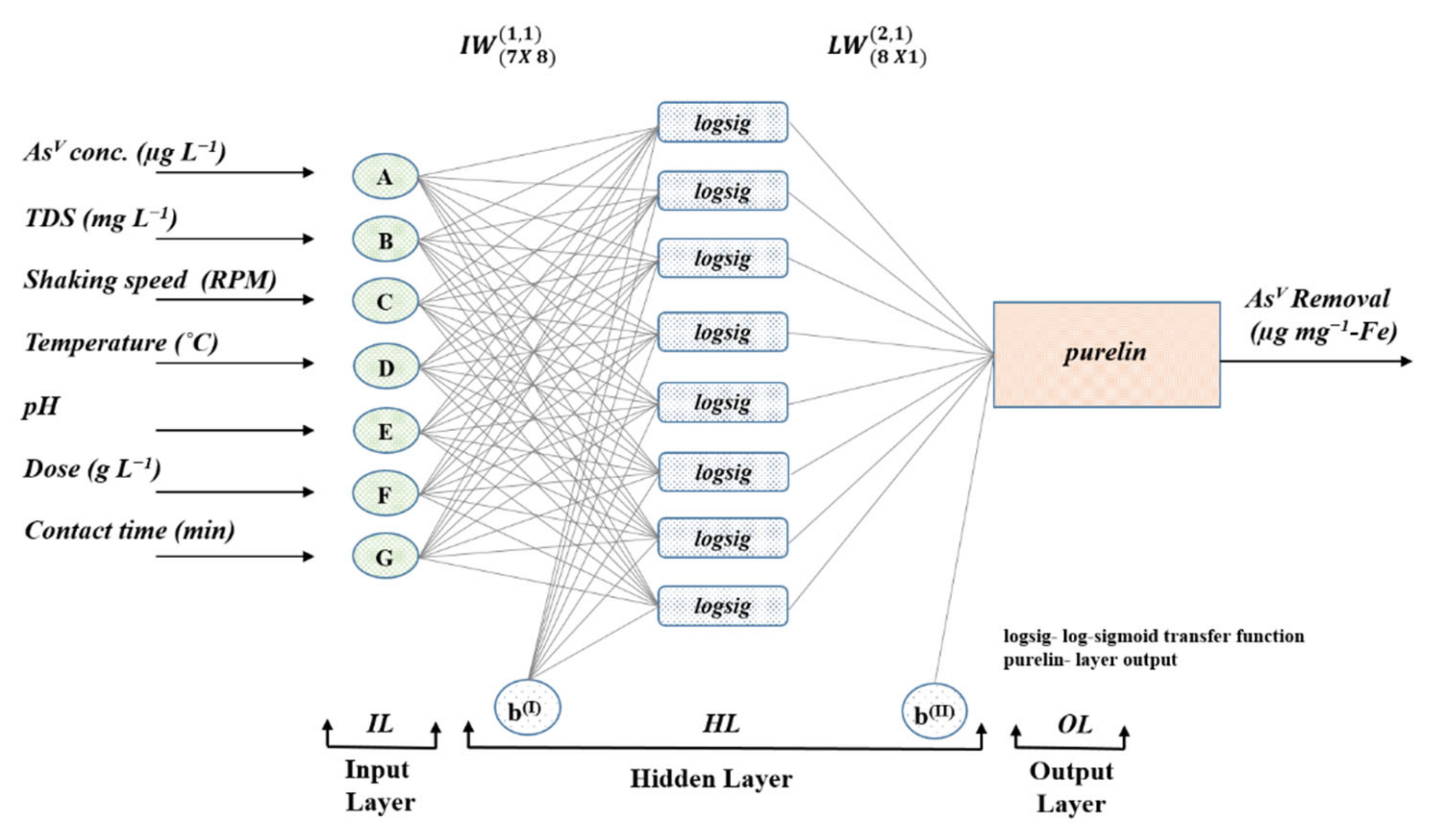
Arsenic removal using nanoparticles requires a robust methodology for predictive analysis. ANN tool can explore input and output parameters effectively. Using the ANN tool, several authors have explored the predictive modeling of arsenic removal by nano adsorbents [102,103]. This tool is appropriate for predicting and estimating adsorption properties due to its complex non-linear characteristics [102,103,104]. The neural network toolbox of MATLAB (version 2013a) was used to predict the adsorption behavior. An approximation algorithm based on feed-forward backpropagation was applied in which the mean square error represents the accuracy index. The three-layered architecture of the backpropagation neural network (BPNN) represented as IL-HL-OL is shown in Figure 3. Where IL is input nodes (equal to the number of variables in the model), HL is hidden nodes (optimized using runs), and OL is output nodes (based on numbers). A topology network architecture is illustrated below:

3. Results and Discussion

3.1. Characterization of Maghemite Nano-Particles

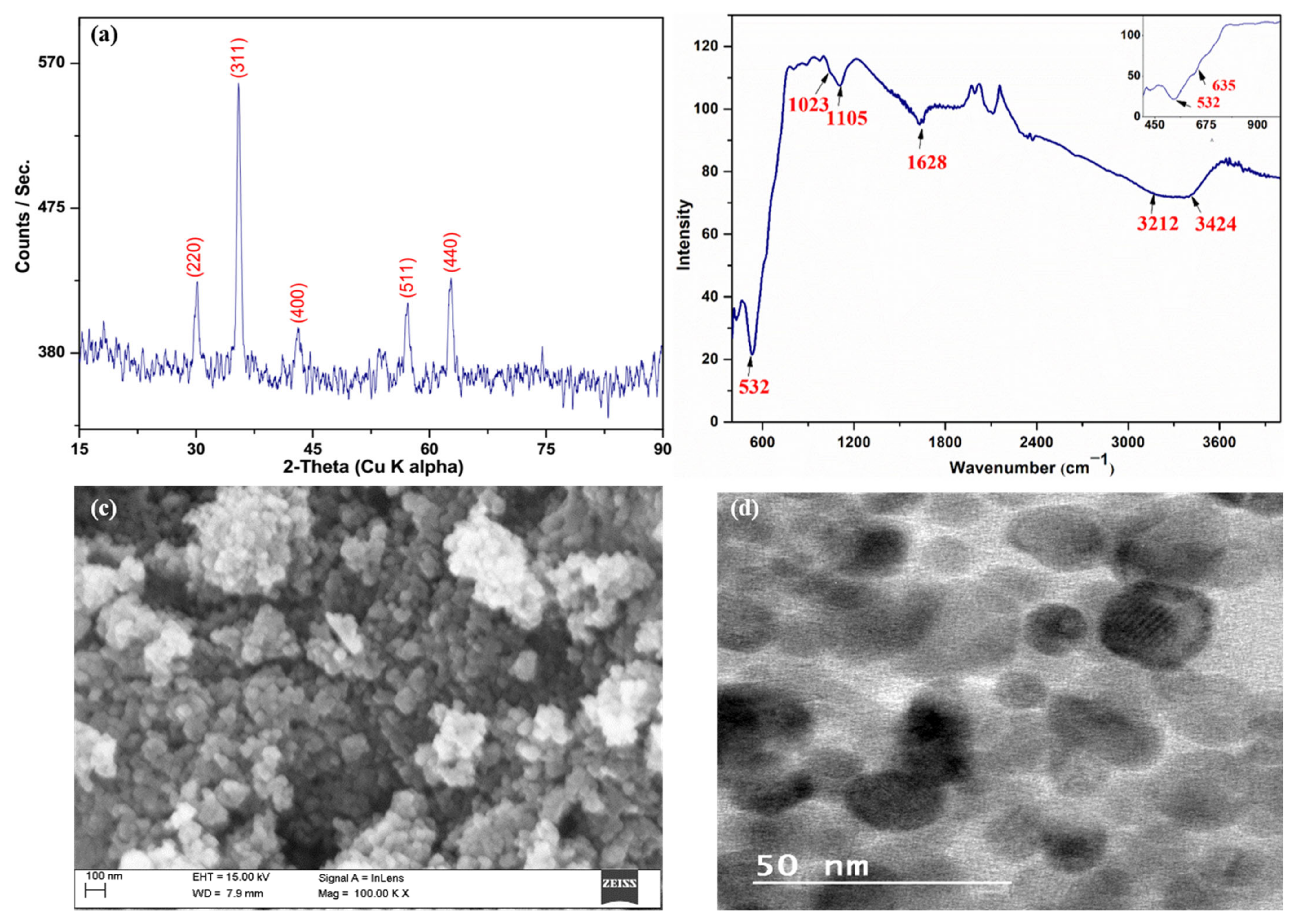
XRD analysis (Figure 4a) confirmed that the observed diffraction patterns matched with the (220), (311), (400), (511), and (440) diffraction of the cubic structure of γ-Fe₂O₃ (JCPDS file no. 39-1346). Using Scherrer’s equation, the calculated average crystallite size was 15 ± 3 nm (Table S1). The recorded FTIR spectrum shows several peak(s) (cm⁻¹) at 532, 635, 1023, 1105, 1620, 3212 and 3424 (Figure 4b), similar to those reported earlier for MNPs [80,105]. A broad peak area of 3200–3600 cm⁻¹ is characteristic of large surface hydroxyl moieties (Table S2).

Figure 4c, FESEM image shows that prepared MNPs are not spherical and monodispersed. It also suggested agglomerates formation in prepared MNPs. It is possibly due to the solid magnetic interactions among nanoparticles. Figure 4d. shows the TEM image of MNPs. By analyzing several TEM images, the estimated average particle size (nm) was calculated to be 16 ± 9 nm, which agrees with the particle size calculated from the XRD analysis.

3.2. Elemental Characterization of Groundwater and Its Formulation

The analyzed chemical composition of collected groundwater’s from locations I and II are shown in

Table 5. Physio-chemical analyses of actual groundwater of Ballia district (two locations) used for artificial water formulations.

Parameter	Unit	Method of Test	DL *	PL *	Location I	Location II
pH	pH unit	pH probe	6.5–8.5	NR	7.45 ± 0.1	7.34 ± 0.1
Electrical conductivity	µS cm−1	EC probe	-	-	341 ± 6	1524 ± 7
TDS	mg L−1	TDS probe	500	2000	435.9 ± 4	1590.6 ± 4
Total hardness	mg L−1	Titrimetric	300	600	160 ± 4	424 ± 4
Alkalinity	mg L−1	Titrimetric	200	600	86 ± 3	222 ± 4
Bicarbonate (as CaCO3)	mg L−1	Titrimetric	-	-	27 ± 2	115.3 ± 1.5
Phosphate (as PO43−)	mg L−1	Spectrophotometric			0.91 ± 0.1	2.02 ± 0.1
Silica (as H4SiO4)	mg L−1	Spectrophotometric			18.4 ± 2	42.4 ± 1
Sodium (as Na+)	mg L−1	IC	-	-	32.4 ± 1	169.4 ± 1
Potassium (as K+)	mg L−1	IC	-	-	15.3 ± 0.2	94.7 ± 1
Fluoride (as F−)	mg L−1	IC	1.0	1.5	1.54 ± 0.1	3.04 ± 0.1
Chloride (as Cl−)	mg L−1	IC	250	1000	132.4 ± 1	435.2 ± 1
Calcium (as Ca2+)	mg L−1	IC	75	200	28.9 ± 0.4	185.1 ± 1
Magnesium (as Mg2+)	mg L−1	IC	30	100	26.8 ± 1	32.4 ± 1
Sulphate (as SO42−)	mg L−1	IC	200	400	30.4 ± 1.2	220.4 ± 2
Nitrate	mg L−1	IC	45	NR	20.0 ± 0.4	140.0 ± 1
Iron	mg L−1	ICP-MS	0.3	1.0	0.53 ± 0.02	0.37 ± 0.03
Manganese	mg L−1	ICP-MS	0.1	0.3	2 ± 0.1	3.03 ± 0.1
Copper	mg L−1	ICP-MS	0.05	1.5	ND	ND
Lead	mg L−1	ICP-MS	0.01	NR	ND	ND
Cadmium	mg L−1	ICP-MS	0.003	NR	ND	ND
Zinc	mg L−1	ICP-MS	5	15	2 ± 0.1	3.96 ± 0.3
Arsenic (as Total)	µg L−1	MP-AES	10	50	54 ± 2	200 ± 1

As per Indian Standard: 10,500 (2012), NR, no relaxation; ND, not determined; * DL, desirable limit; * PL, permissible limit; IC, Ion chromatogram; ICP-MS, inductively coupled plasma mass spectroscopy; MP-AES, Microwave plasma atomic emission spectroscopy.

. The validation of formulated water in terms of accuracy was also performed by analyzing respective ion concentrations.

3.3. Characteristics of Arsenic Removal in the Multi-Ionic System

The experimental runs examined the As^V adsorption of MNPs under the specified conditions, as mentioned by Taguchi’s L₂₇ OA (Table 4). Three experiments were performed in each run, indicating different parametric conditions. The increasing difference between the assigned level values indicates the growing influence of that experimental variable on the removal capacity. The above-listed parameters (in Table 2) demonstrated notable effects on As^V removal. These effects are discussed individually below:

3.3.1. Effects of Process Parameters: Shaking Speed, Temperature, and Contact Time

The lower value of q_e (µg mg⁻¹-Fe) at levels L₁ (1.09) and L₃ (1.21) as compared to that of level L₂ (1.53) indicates that a variation in shaking speed is affecting the As^V removal (

Table 6. Adsorption capacities (q_e, µg mg⁻¹-Fe) and associated signal noise (S:N, dB) ratio determined three value levels for each variable.

	Raw Data, Average Value			Main Effects, Raw Data		S:N Ratio (dB), Average Value			S:N Ratio (dB), Main Effects
Factor	L1	L2	L3	L2–L1	L3–L2	L1	L2	L3	L2–L1	L3–L2
A	0.6	1.3	2.0	0.7	0.8	−6.4	−0.2	3.9	6.3	4.0
B	1.8	1.0	1.0	−0.8	Nil	1.8	−2.6	−1.9	−4.4	0.7
C	1.1	1.5	1.2	0.4	−0.3	−2.1	0.5	−1.2	2.6	−1.7
D	2.2	0.9	0.8	−1.3	−0.2	3.7	−2.5	−3.9	−6.1	−1.5
E	0.9	1.2	1.7	0.3	0.5	−1.5	−2.1	0.9	−0.5	2.9
F	1.8	1.3	0.8	−0.5	−0.5	1.4	Nil	−4.1	−1.4	−4.1
G	1.1	1.3	1.4	0.2	0.1	−0.5	−0.4	−1.8	0.1	−1.4
A.B	2.2	2.8	2.7	0.7	−0.1	−2.5	−0.5	−2.4	2.0	−1.9
A.C	2.8	2.3	2.6	−0.5	0.3	−2.3	−2.5	−0.7	−0.2	1.9
B.C	2.2	2.8	2.7	0.6	−0.1	−0.6	−3.6	−1.2	−3.0	2.4

* A.B (As^V conc. × TDS); A.C (As^V conc. × shaking speed); B.C (TDS × shaking speed).

. This decrease in the removal capacity can be attributed to the desorption of adsorbed As^V into the aqueous solution at a high shaking speed. The formation of an external boundary layer of adsorbed species on the adsorbent and the distribution of remaining solute(s) in bulk are significant factors affecting adsorption phenomena [106,107]. This study suggests that external diffusion is likely the rate-limiting step in adsorption [86]. Further, the low adsorption capacity value for L₁ ensures that nanoparticles were not entirely homogenously suspended in the solution at the shaking speed of <170 rpm.

An increase in the temperature from 10 to 30 °C causes a monotonic decrease in the adsorption capacity, indicating the low heat of adsorption during the removal process. The maximum value (1.41 µg mg⁻¹-Fe) of adsorption capacity is observed for a high contact time (L₃). This outcome also suggests that physical absorption is the predominating phenomenon and hydroxyl groups and AsV interacts with weak electrostatic interactions.

3.3.2. Effects of Process Parameters: As^V Concentration, TDS, and pH

An increase in the As^V initial concentration (A) from 55 to 200 µg L⁻¹, the adsorption capacity (q_e) was observed to increase, and the maximum adsorption capacity was observed at 200 µg L⁻¹ (level L₃). The competition for ion concentration causes an increase in adsorption capacity (0.55 to 2.02 µg mg⁻¹-Fe), which is due to a decrease in the hindrance for the uptake of As^V ions as the mass-transfer operating force gets intensified.

Increasing TDS (B) from (L₁ to L₃) 436 to 1591 mg L⁻¹, the adsorption capacity (q_e) was observed to decrease (1.8 to 1.0). It apparently occurred due to the competition among As^V and other ions to occupy the vacant sites of the nanoparticle surface. However, a variation in adsorption capacity was observed, which could be due to the dominating effect of different competing ions leading to negligible adsorption of As^V beyond the TDS concentration of 1014 mg L⁻¹ (L₂).

The As^V adsorption increases from 0.9 to 1.7 µg mg⁻¹-Fe with an increase in pH. The effect of various parameters on the adsorption capacity has been observed to follow a decreasing order as total dissolved solids (B) > arsenate concentration (A) > dose (F) > pH (E) and arsenate concentration (A) > pH (E) > dose (F) > total dissolved solids (B), respectively. It may be due to the occurrence of charged species of As^V beyond the near-neutral pH conditions. The results thus indicate a strong effect of the total dissolved solids concentration on the adsorption process and the role of the occurrence of a change in the surface moieties on electrostatic interactions. Few authors have reported an increase in the removal capacity of nanoparticles in the presence of ions such as nitrates and bicarbonates [69].

3.4. Analysis of Inter-Parametric Interactions

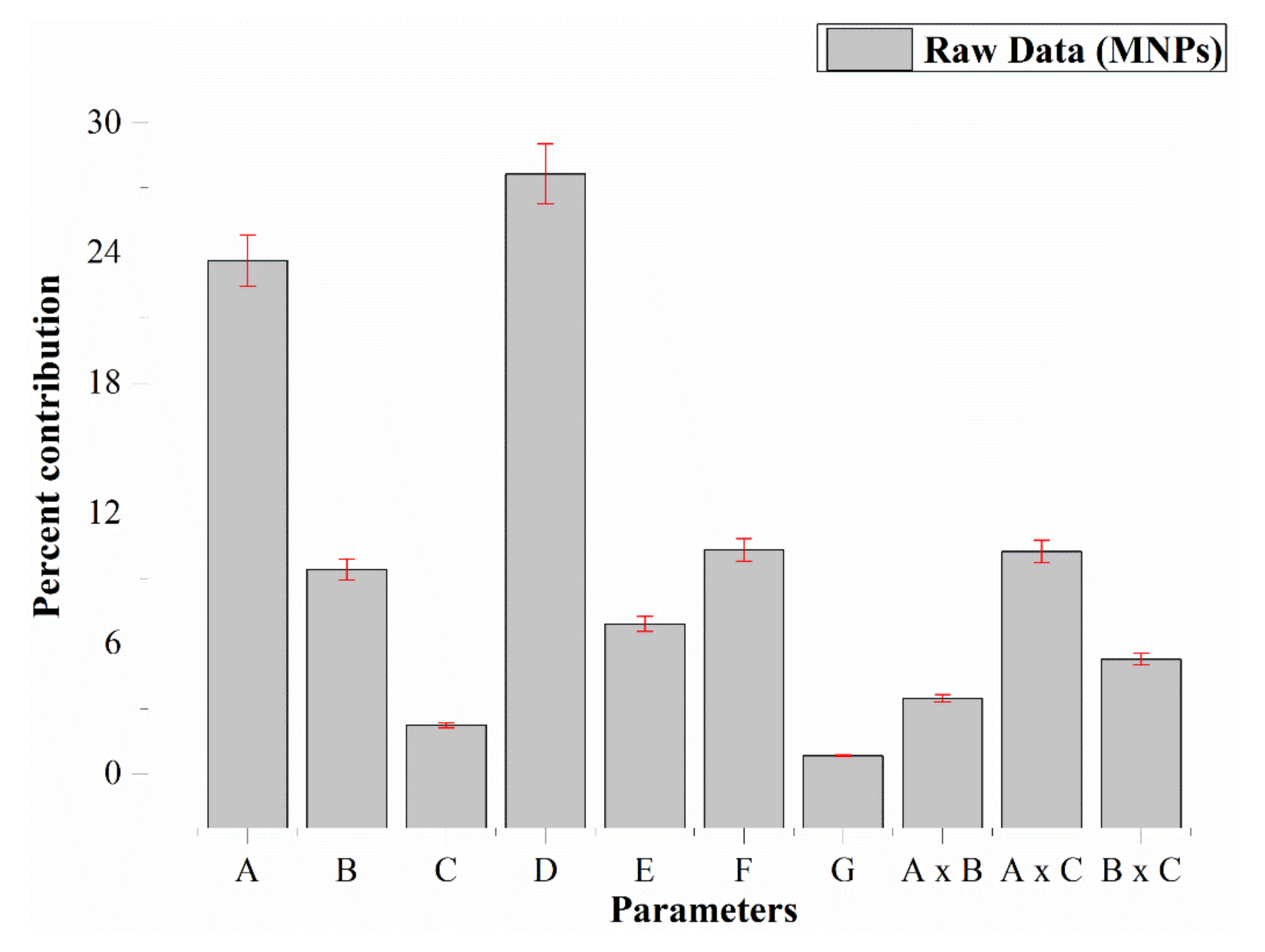
The ANOVA outcomes for raw and S:N data and the percentage contribution of individual process parameters affecting the As^V adsorption are presented in

Table 7. ANOVA of q_e (µg mg⁻¹-Fe) and S:N (dB) ratio data for the multi-ionic system in the adsorption of As^V using MNPs.

	Raw Data					S:N ratio
Parameter	Sum of Square	DOF a	Mean Square	F Value	% Contrib.	Sum of Square	DOF a	Mean Square	F Value	% Contrib.
A	29.3	2	14.6	292.7	23.66	485.67	2	242.84	933.98	39.7
B	11.7	2	5.9	117.4	9.41	98.66	2	49.33	189.73	8.1
C	2.8	2	1.4	27.9	2.23	31	2	15.5	59.62	2.5
D	34.3	2	17.2	343.4	27.65	290.58	2	145.09	558.81	23.7
E	8.5	2	4.3	85.3	6.90	43.69	2	21.85	84.02	3.6
F	12.9	2	6.4	128.5	10.32	146.46	2	73.23	281.65	12.0
G	1.0	2	0.5	10.4	0.83	11.77	2	5.89	22.63	1.0
A x B	8.8	4	2.2	43.8	3.48	39.64	4	9.91	38.12	1.6
A x C	25.6	4	6.4	127.4	10.25	108.93	4	27.23	104.74	4.5
B x C	13.2	4	3.3	65	5.27	85.48	4	21.37	82.19	3.5
Residual	0.08	54	0.06			0.52	2	0.26
Model	124.10	26	62.09			1341.08	24	612.69	2356.5
Corr. Total	124.18	80	62.15			1341.60	26	612.43

DOF ^a—Degree of freedom. Sum of square—DOF × mean square.

. Figure 5 shows the variations in the adsorption capacity as a function of the As^V initial concentration for the different TDS levels. With an increase in TDS (L₁ to L₃), the adsorption capacity increases with increasing As^V concentration. It might be due to the secondary sites developed for As^V adsorption provided by the surface complexes produced with other ions.

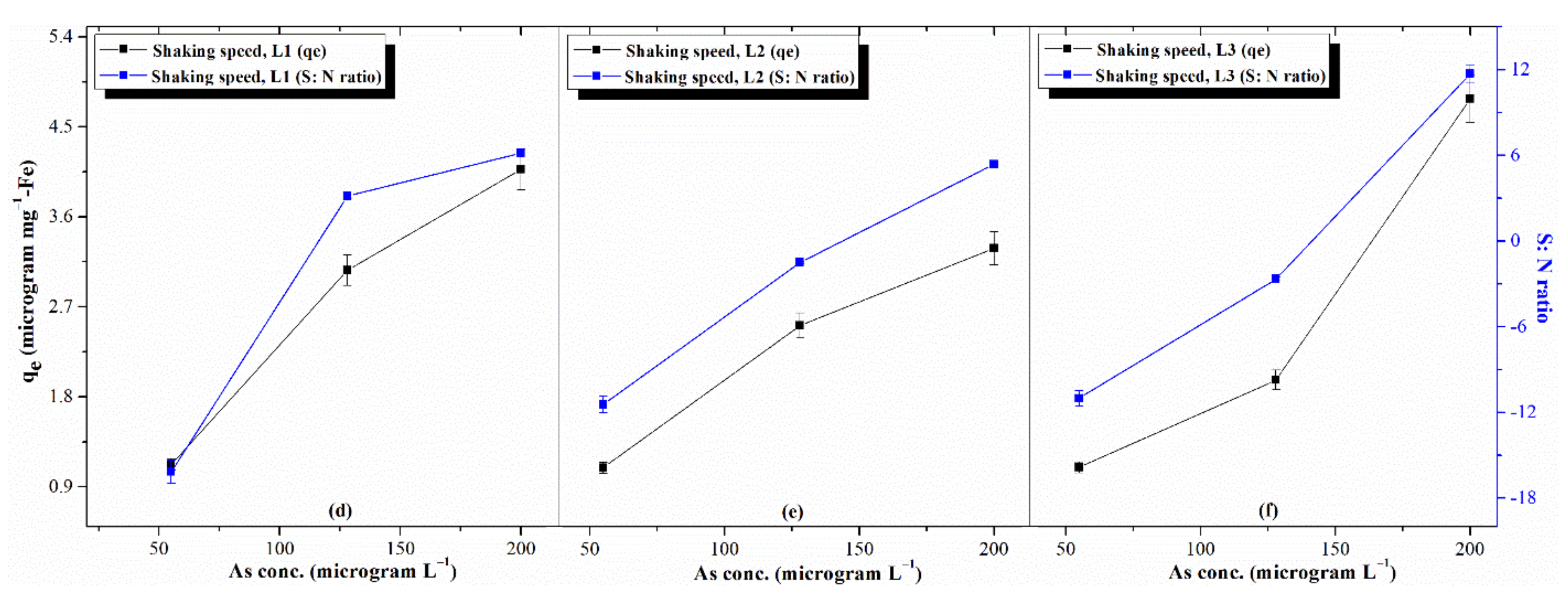
Figure 6 depicts the variations in the adsorption capacity as a function of the initial concentration of As^V at each level of shaking speed. At a low concentration of As^V (L₁-55 µg L⁻¹), the shaking speed was examined to affect its removal. An antagonistic behavior of its removal was observed beyond the As^V concentration of (L₁) 55 µg L⁻¹. A low removal capacity of As^V was found at the shaking speed of 170 rpm (L₂) for MNPs. Further, the combined effect of shaking speed and TDS was explored on the As^V removal (Figure 7). An insignificant variation in the removal capacity at low shaking speed for the whole range of TDS (436–1591 mg L⁻¹) ensured that nanoparticles were not homogeneously suspended in the solution at a shaking speed of <170 rpm. It indicates that external diffusion is likely to be the rate-limiting step in adsorption. However, high removal capacity was observed at high TDS and a shaking speed of 170 rpm. The inter-parametric interaction studies revealed that the As^V removal onto MNPs occurred through the formation of surface complexes.

The pH_PZC (point of zero charge) of the adsorbing material and the charge of the contaminants are essential factors that affect their removal from aqueous solutions. This study found the pH_PZC for these nanoparticles in the acidic range (pH_PZC—2.8). The surface moieties (primarily hydroxyl) acquired a negative charge between pH 7–9. Figure S5. indicates the zeta potential analysis (ζ) with a value of −33 ± 0.6 mV at near-neutral pH conditions, considered colloidal stable. Therefore, the adsorption of arsenic species occurred through weak electrostatic interactions. The reaction mechanisms explaining the development of surface charge onto these MNPs are mentioned below:

$$\mathrm{Fe}-\mathrm{O}-\mathrm{H}+{ \mathrm{H}}^{+}\stackrel{ \mathrm{pH} <{ \mathrm{pH}}_{\mathrm{PZC} }}{\to } \mathrm{Fe}-{\mathrm{O}}^{+}{\mathrm{H}}_2(\mathrm{pH}<2.8)$$

(11)

$$\mathrm{Fe}-\mathrm{O}-\mathrm{H}+{ \mathrm{OH}}^{-} \stackrel{ \mathrm{pH} >{ \mathrm{pH}}_{\mathrm{PZC} }}{\to } \mathrm{Fe}-{\mathrm{O}}^{-}+{ \mathrm{H}}_2\mathrm{O} \left(\mathrm{pH} 7-9\right)$$

(12)

$$\mathrm{Fe}-\mathrm{O}-\mathrm{H} +{ \mathrm{H}}^{+}+2\left(\mathrm{H}-\mathrm{OH}\right)\stackrel{ \mathrm{pH} >{ \mathrm{pH}}_{\mathrm{PZC} }}{\to } \mathrm{Fe}-{\mathrm{O}}^{-}+2{\mathrm{H}}_3{\mathrm{O}}^{+}\left(\mathrm{pH} 6.1-7.0\right)$$

(13)

3.5. Selection of Optimal Levels and Estimation of Response Characteristics

Higher values of q_e represent better arsenic removal, so optimal levels to maximize q_e were determined. The percent contribution of individual process parameters and parametric interaction on the As^V removal capacity are presented in Figure 8. The optimized conditions for the location I and Location II were A₁, B₁, C₂, D₁, E₃, F₁, G_3, and A₃, B₃, C₂, D₁, E₃, and F₁, G₃, respectively. Thus, the significant process parameters that affected the As^V removal by MNPs and their optimal levels are included as Location I (A₁, B₁, C₂, D₁, E₃, F₁, G₃), location II (A₃, B₃, C₂, D₁, E₃, F₁, G₃) and experimental design (A₃, B₁, C₂, D₁, E₃, F₁, G₃). The estimated value of adsorption capacity using the optimal levels (as already selected) was calculated from Table 6. These are given as below:

• The first level of concentration of As^V ions (${\overline{\mathbf{A}}}_{\mathbf{1}}$) = 0.6
• The third level of concentration of As^V ions (${\overline{\mathit{A}}}_{\mathbf{3}}$) = 2.0
• The first level of concentration of TDS (${\overline{\mathit{B}}}_{\mathbf{1}}$) = 1.8
• The third level of concentration of TDS (${\overline{\mathit{B}}}_{\mathbf{3}}$) = 1.0
• A second level of shaking speed (${\overline{\mathit{C}}}_{\mathbf{2}}$) = 1.5
• The first level of temperature (${\overline{\mathit{D}}}_{\mathbf{1}}$) = 2.2
• The third level of pH (${\overline{\mathit{E}}}_{\mathbf{3}}$) = 1.7
• The first level of dose concentration (${\overline{\mathit{F}}}_{\mathbf{1}}$) = 1.8
• The third level of contact time (${\overline{\mathit{G}}}_{\mathbf{3}}$) = 1.4

The overall mean for the total removal capacity (${\overline{T}}_{MNPs}$) is 1.28 (from Table 4). The calculated predicted optimum values (µ) for removal capacity for location I, location II and experimental design are given as Equations (14)– (16) below:

$${\mu }_{\mathrm{Location} \mathrm{I}}=3.2{ \mu \mathrm{g} \mathrm{mg}}^{-1}-\mathrm{Fe}$$

(14)

$${\mu }_{\mathrm{Location} \mathrm{II}}=3.8{ \mu \mathrm{g} \mathrm{mg}}^{-1}-\mathrm{Fe}$$

(15)

$${\mu }_{{\mathrm{q}}_{\mathrm{e},\max .}}=4.6{ \mu \mathrm{g} \mathrm{mg}}^{-1}-\mathrm{Fe}$$

(16)

Further, the 95% confidence interval for the mean of experimental run outcomes and three conformation experiments (CI_CE and CI_POP) is calculated by substituting the DOF error [f_e = 54 (80–26)], the total number of results [N= 81 (27 × 3)] and the error variance [V_e = 0.06] in Equation (17) to Equation (19):

$${\mathrm{n}}_{\mathrm{effective}}=3$$

(17)

F₀.₀₅ (1, 54) = 4.03 (representing tabulated F-value)

$${\mathrm{CI}}_{\mathrm{CE}}=\pm 0.5$$

(18)

$${\mathrm{CI}}_{\mathrm{POP}}=\pm 0.3$$

(19)

The details of the predicted ranges for the maximum removal capacity at 95% confidence intervals for the location I, location II and experimental design onto MNPs is presented below in

Table 8. Predicted optimal levels of parameters and adsorption capacity (q_e) values, confidence intervals, outcomes of confirmation experiments, and percent variation for location I, location II and experimental design.

	Optimal Levels of Parameters	Predicted Values (µg mg−1-Fe)	Confidence Intervals (95%)	Average (µg mg−1-Fe)	% Variation
Loc. I	A1, B1, C2, D1, E3, F1, G3	3.2	CICE: 2.7 < ${\mu }_{MNPs}$< 3.7 CIPOP: 2.9 < ${\mu }_{MNPs}$< 3.5	3.4 ± 0.04	5.9
Loc. II	A3, B3, C2, D1, E3, F1, G3	3.8	CICE: 4.3 < ${\mu }_{MNPs}$< 3.3 CIPOP: 4.1 < ${\mu }_{MNPs}$< 3.5	3.9 ± 0.09	2.6
qe, max.	A3, B1, C2, D1, E3, F1, G3	4.6	CICE: 5.1 < ${\mu }_{MNPs}$< 4.1 CIPOP: 4.9 < ${\mu }_{MNPs}$< 4.3	4.8 ± 0.02	4.2

.

3.6. Confirmation Experiments

The confirmation experiments for the locations I, II, and q_{e, max}. (overall experimental design) were conducted in triplicate at selected optimal levels of experimental process parameters. Their average values are compared with predicted values, as shown in

Table 9. Calculated speciation of major ionic components for the location I and location II synthetic waters as a function of pH using Visual MINTEQ.

		Location I			Location II
Ionic Species	Molecular Formula	pH 7	pH 8	pH 9	pH 7	pH 8	pH 9
Bicarbonate	HCO3-	81.8	94.6	85.0	81.1	91.7	76.6
Carbonic acid	H2CO3 * (aq.)	16.8	2.0	0.2	15.5	1.8	0.2
Calcium sulfate	CaSO4 (aq.)	6.5	6.5	6.5	19.2	9.1	18.7
Tri-hydrogen ortho-silicate	H3SiO4−	0.2	1.6	13.7	0.2	1.7	14.5
Silicic acid	H4SiO4	99.8	98.4	86.3	99.8	98.3	85.4
Hydrogen phosphate	HPO4−2	35.8	57.9	50.4	34.1	47.2	29.6
Dihydrogen phosphate	H2PO4−	43.1	7.0	0.6	33.6	4.7	0.3
Magnesium phosphate	MgHPO4 (aq.)	11.7	18.9	16.3	7.6	10.4	6.4
Calcium hydrogen phosphate	CaHPO4 (aq.)	5.5	8.9	7.6	17.8	24.5	14.8
Calcium phosphate	CaPO4−	0.2	2.9	22.6	0.7	7.7	46.4
Magnesium phosphate	MgPO4−	-	0.1	0.5	-	0.1	0.2
Hydrogen arsenate	HAsO4−2	57.3	93.0	99.0	62.1	94.2	99.0
Dihydrogen arsenate	H2AsO4−	42.7	6.9	0.7	37.9	5.8	0.6
Arsenate ion	AsO4−3	-	-	0.3	-	-	0.3
Zinc hydroxide	Zn(OH)2 (aq.)	0.1	6.9	78.0	0.1	4.5	64.9
Zinc tri-hydroxide	Zn(OH)3−	-	-	-	-	-	0.3
Magnesium sulfate	MgSO4 (aq.)	2.2	2.2	2.2	7.7	7.7	7.7

. The values of q_e determined through confirmation experiments were found within the 95% confidential interval of CI_CE for MNPs. These optimal values are valid only within the range of designated process parameters. However, it is proposed to explore the removal capacity through additional confirmation experiments during interpolation/exploitation.

3.7. Analysis Using Visual MINTEQ

Generally, several inorganic species (ionic or complexion) are formed when a solution is allowed to be prepared by mixing the salts with different solubility product values. Among those, few were discussed, which might potentially affect the adsorption of As^V onto MNPs. The percentage distribution of species for ions considered in the synthetic water formulation (as in Table 1) is shown in Table 9.

The ionic species of As^V in the aqueous solution were reported to be HAsO₄²⁻, H₂AsO₄, and AsO₄³⁻. At high As^V concentration and pH value, an increase in the adsorption capacity for As^V was examined. In addition, the percentage of the dominant arsenic specie (HAsO₄⁻²) predominantly affects the removal of As^V and has more potential for adsorption onto MNPs.

Phosphate ions have been reported to have significant potential as a competing molecule to arsenic adsorption [37,56,108]. In the present study, its ionic and neutral species, such as HPO₄²⁻, H₂PO₄⁻, CaPO₄⁻, MgPO₄⁻, MgHPO₄, and CaHPO₄, were considered competing species. It is because of their shared charge value of 1.25 that is equivalent to As^V. At pH 9, the HPO₄²⁻ oxyanion was the primary competing specie. Its percentage distribution values for the formulated water (Location I and II) were 50.4 and 29.6, respectively. This percentage distribution decreased due to the conversion of HPO₄²⁻ and H₂PO₄⁻ competing ions into CaPO₄⁻ species. However, these values are comparatively less than those observed for pH values 7 and 8. This interpretation favors a high adsorption capacity observed at a high pH. The ion/complex ions such as H₃SiO₄⁻, H₄SiO₄, Zn(OH)₂, and Zn(OH)₃⁻ were identified as competing species due to the smaller values of their shared charge than As^V. Moreover, H₃SiO₄⁻ might also be responsible for decreasing the adsorption capacity at a high pH value.

4. Surface Complexation Models (SCMs) for Adsorption Behavior

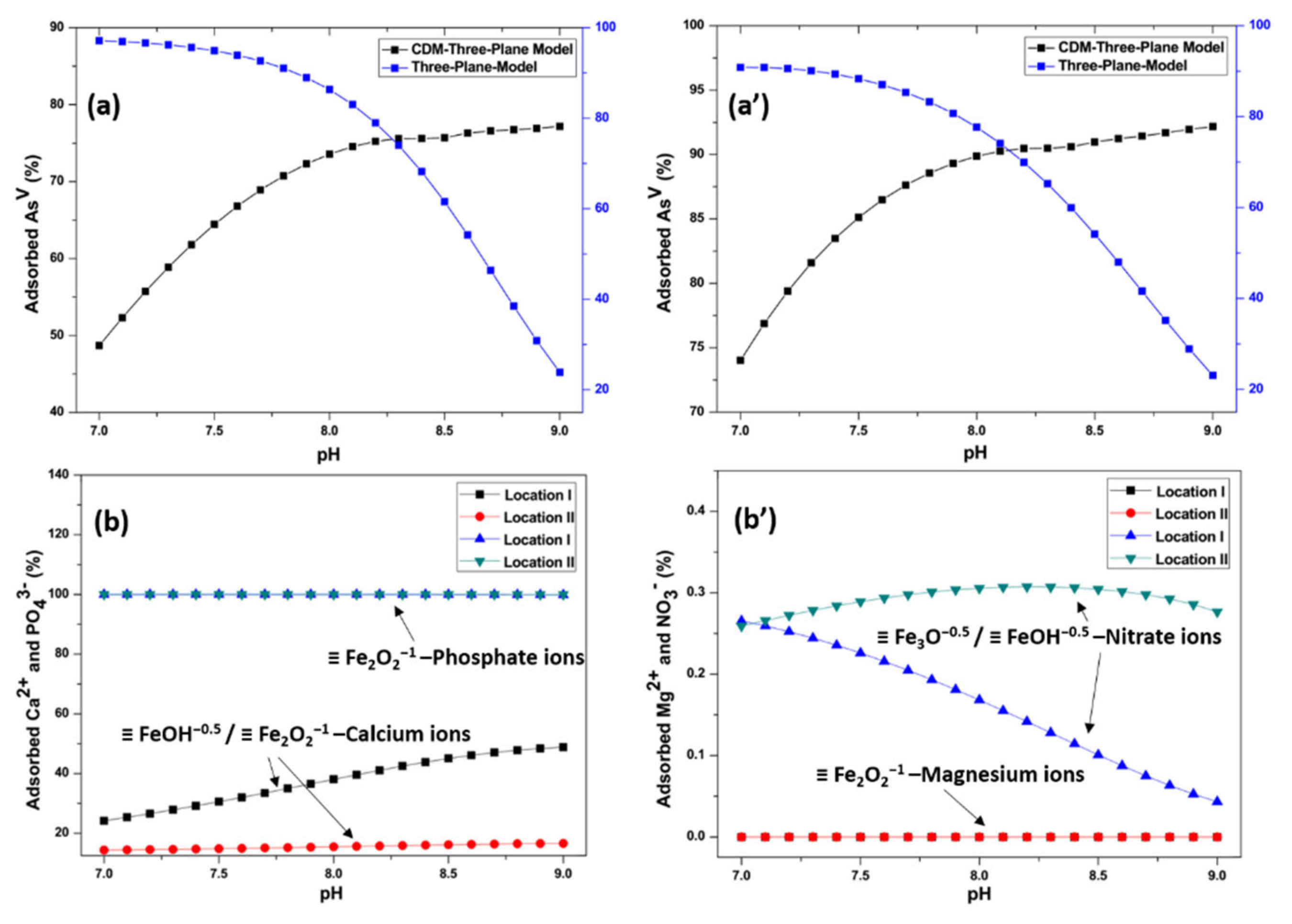
Generally, the hydroxyl moieties, such as single [(OH)₃-Fe-Fe-R] and double [(OH)₃-Fe-H₃O₃-R] coordinated hydroxyls, have been reported for iron^III oxide(s) nanoparticles [109], and the double joint surface hydroxyls were previously demonstrated to be remarkably stable and unreactive [110]. Trainor et al. [110] have shown that the singly and triple coordinated hydroxyls are more reactive towards cationic species due to their efficient proton lability. Therefore, the CD-MUSIC model, along with 2pk-TPM, was used to explore controls of surface speciation on adsorption, involving the reactivity of singlet (FeOH^−0.5) and triplet (Fe₃O^−0.5) iron species. This study provided surface complexation modeling by considering the surface species summarized in Table 3. Figure 9 shows that phosphate ions compete with As^V for adsorption in the whole pH range, whereas calcium ions counter the adsorption at high pH and low concentration. The study revealed that the phosphate ions have a more significant impact on the As^V adsorption than calcium and nitrate ions. In contrast, magnesium ions did not significantly affect As^V adsorption.

5. ANN Predictions

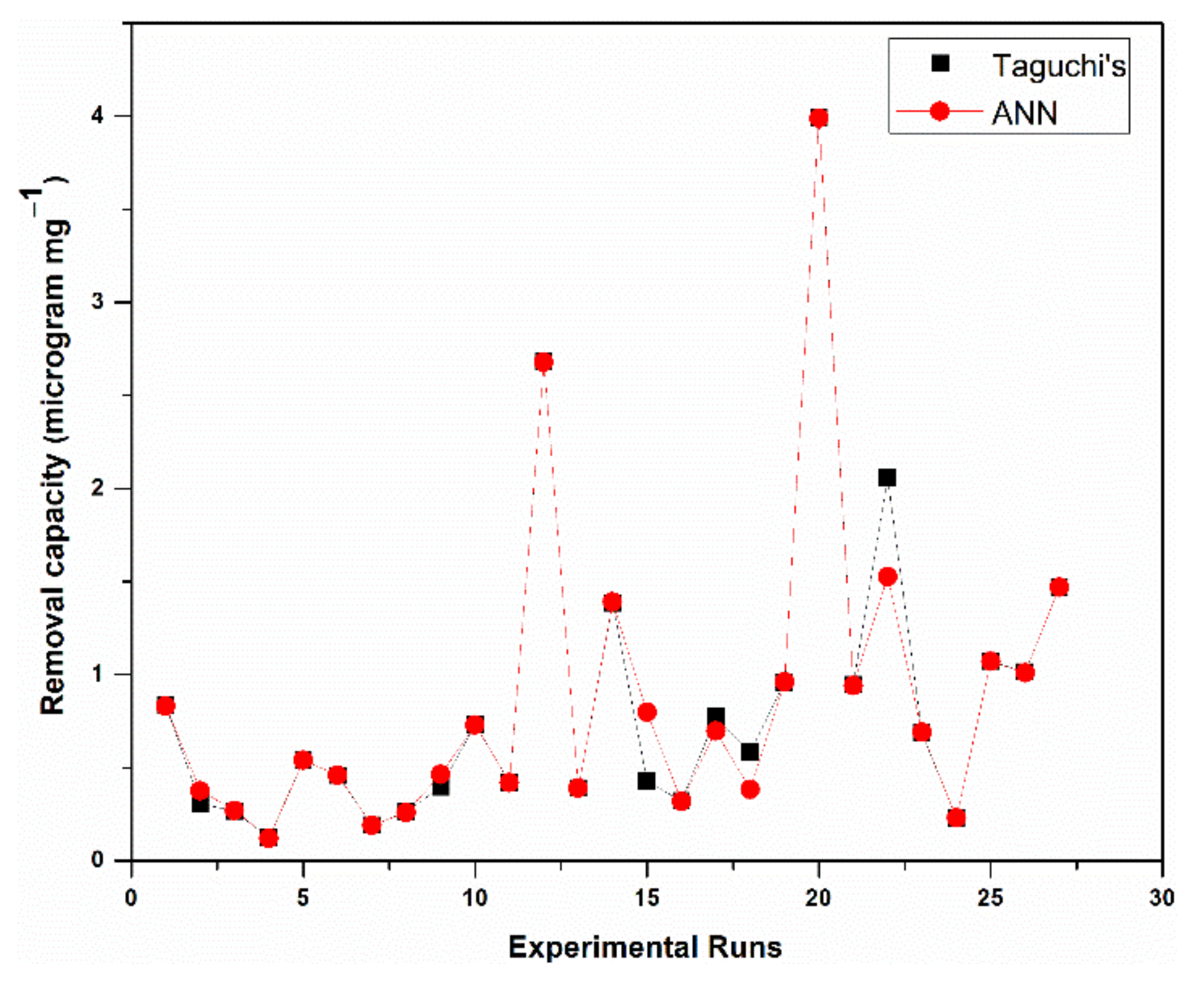
The ANN model was explored to compare Taguchi’s experimental outcomes and ANN-generated response values for adsorption capacity for all the experimental runs. A three-layer feed-forward network using a hyperbolic function (tangent) under a standardized method was applied for the predictive analysis. Out of 27 experimental sets, 21 datasets (80%) were used to train the network, and the remaining 20% were used to validate and test the ANN model. The network was trained to get the minimum mean square error, achieved after 309 iterations. The details of their weights and biases are shown in Table S5. A plot was generated to compare the experimental outcomes of batch experiments and the optimized generated values through the ANN model, as shown in Figure 10. There was significant agreement between the outcomes of Taguchi’s model and ANN predicted values, with a mean squared error of 0.0174. For the present study, ANN was found to be an effective tool for the predictive modeling of As^V removal using MNPs.

6. Conclusions

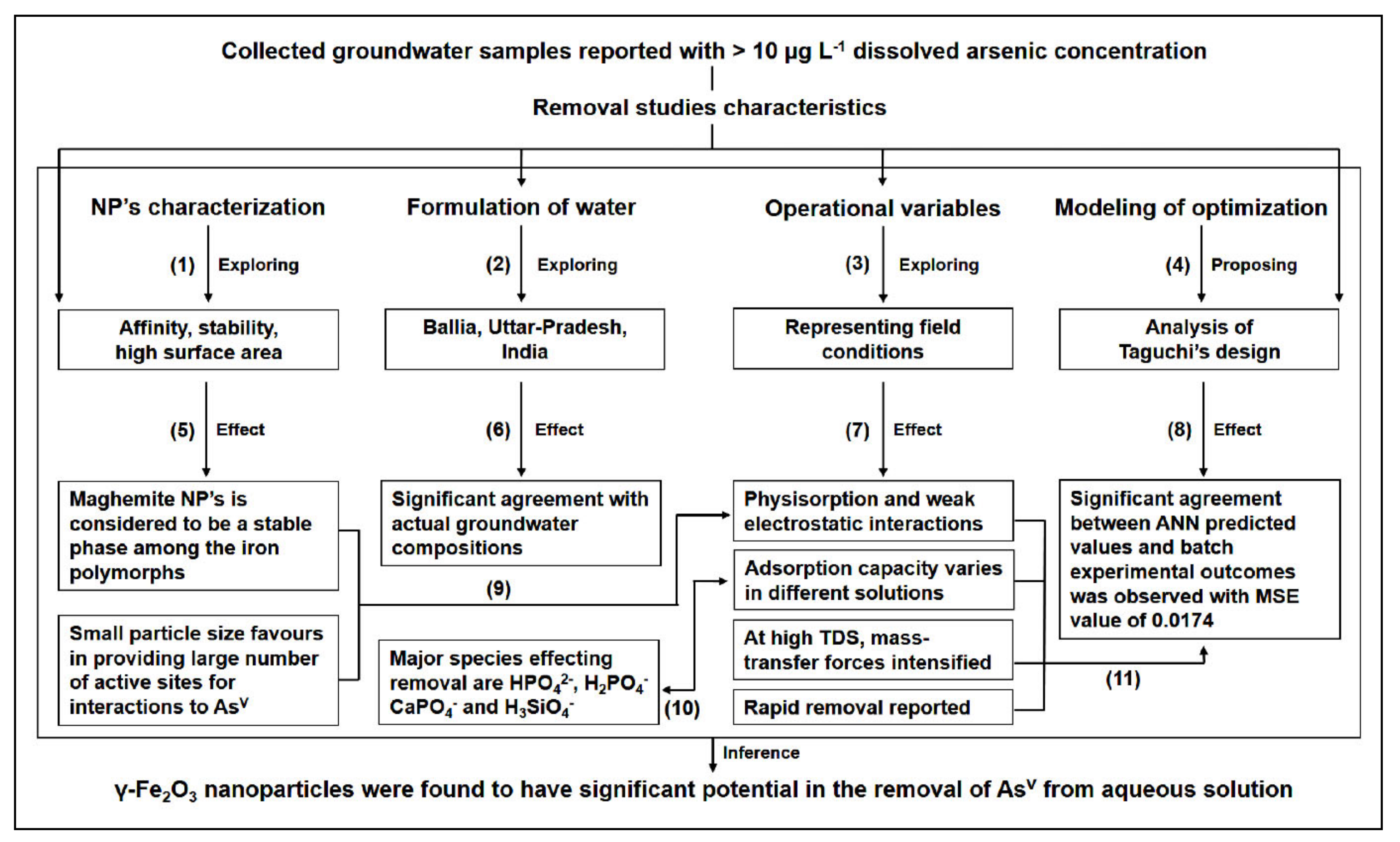
The adsorption capacity of an iron^III oxide polymorph was investigated for As^V removal in the synthetic water samples, simulating the arsenic-infested groundwater of Ballia district, Uttar Pradesh, India. The developed MNPs were observed as polycrystalline with an average particle size of 14.6 ± 2.4 nm. The pHpzc value of 2.8 indicates that MNPs carry negatively charged surface moieties singlet (FeOH^−0.5) and triplet (Fe₃O^−0.5) species in the investigated pH range of adsorption studies. At optimized conditions, the maximum adsorption of MNPs was examined as 4.2 µg mg⁻¹-Fe. The ionic/complex species, such as HPO₄⁻², H₂PO₄⁻, CaPO₄⁻, MgPO₄⁻, H₃SiO₄⁻, Zn(OH)₃⁻, MgHPO₄ and CaHPO₄ H₄SiO₄, Zn(OH)₂, were identified as competing ions to As^V adsorption. The phosphate ions were identified as major competing ions during the adsorption process. However, nitrate ions were observed to impact the adsorption behavior in the pH and TDS range under investigation. The ANN predicted values were closely matched with Taguchi’s experimental outcomes at a mean square error (MSE) of 0.0174 µg mg⁻¹-Fe. The outcomes of this work is presented in Figure 11. These nanoparticles were reported to have a significant potential for As^V removal and can be applied in the ex-situ treatment units of the arsenic-affected areas. Considering the redox-sensitive nature of arsenic species, investigations related to the formation of chemical processes, surface complexation, and mineral precipitation reactions should be considered for future studies.

References

- World Health Organization. Exposer to Arsenic: A Major Public Health Concern. Report World Health; World Health Organization: Geneva, Switzerland, 2010. [Google Scholar]
- Raposo, J.C.; Sanz, J.; Zuloaga, O.; Olazabal, M.A.; Madariaga, J.M. Validation of the Thermodynamic Model of Inorganic Arsenic in Non Polluted River Waters of the Basque Country (Spain). Talanta 2004, 63, 683–690. [Google Scholar] [CrossRef] [PubMed]
- Vahter, M. Health Effects of Early Life Exposure to Arsenic. Basic Clin. Pharmacol. Toxicol. 2008, 102, 204–211. [Google Scholar] [CrossRef] [PubMed]
- Mohammed Abdul, K.S.; Jayasinghe, S.S.; Chandana, E.P.S.; Jayasumana, C.; De Silva, P.M.C.S. Arsenic and Human Health Effects: A Review. Environ. Toxicol. Pharmacol. 2015, 40, 828–846. [Google Scholar] [CrossRef]
- Smedley, P.L.; Kinniburgh, D.G.; Macdonald, D.M.J.; Nicolli, H.B.; Barros, A.J.; Tullio, J.O.; Pearce, J.M.; Alonso, M.S. Arsenic Associations in Sediments from the Loess Aquifer of La Pampa, Argentina. Appl. Geochemistry 2005, 20, 989–1016. [Google Scholar] [CrossRef]
- Ahmed, M.F. An Overview of Arsenic Removal Technologies in Bangladesh and India. In Proceedings of the BUET-UNU International Workshop on Technologies for Arsenic Removal from Drinking Water, Dhaka, Bangladesh, 5–7 May 2001. [Google Scholar]
- Ciminelli, V.S.T.; Gasparon, M.; Ng, J.C.; Silva, G.C.; Caldeira, C.L. Dietary Arsenic Exposure in Brazil: The Contribution of Rice and Beans. Chemosphere 2017, 168, 996–1003. [Google Scholar] [CrossRef] [PubMed]
- Bondu, R.; Cloutier, V.; Rosa, E.; Benzaazoua, M. Mobility and Speciation of Geogenic Arsenic in Bedrock Groundwater from the Canadian Shield in Western Quebec, Canada. Sci. Total Environ. 2017, 574, 509–519. [Google Scholar] [CrossRef] [PubMed]
- Polya, D.; Gault, A.G.; Diebe, N.; Feldman, P.; Rosenboom, J.; Gilligan, E.; Cooke, D. Arsenic Hazard in Shallow Cambodian Groundwaters. Mineral. Mag. 2005, 69, 807–823. [Google Scholar] [CrossRef]
- Pino, P.; Iglesias, V.; Garreaud, R.; Cortés, S.; Canals, M.; Folch, W.; Burgos, S.; Levy, K.; Naeher, L.P.; Steenland, K. Chile Confronts Its Environmental Health Future After 25 Years of Accelerated Growth. Ann. Glob. Health 2015, 81, 354–367. [Google Scholar] [CrossRef]
- Adomako, E.E.; Williams, P.N.; Deacon, C.; Meharg, A.A. Inorganic Arsenic and Trace Elements in Ghanaian Grain Staples. Environ. Pollut. 2011, 159, 2435–2442. [Google Scholar] [CrossRef]
- Sugár, É.; Mihucz, V.G.; Záray, G. Determination of Arsenic in Drinking Water and Several Food Items. Elelmiszervizsgalati Kozlemenyek 2014, 60, 163–176. [Google Scholar]
- Navarro, O.; González, J.; Júnez-Ferreira, H.E.; Bautista, C.F.; Cardona, A. Correlation of Arsenic and Fluoride in the Groundwater for Human Consumption in a Semiarid Region of Mexico. Procedia Eng. 2017, 186, 333–340. [Google Scholar] [CrossRef]
- Berg, M.; Stengel, C.; Trang, P.; Hungviet, P.; Sampson, M.; Leng, M.; Samreth, S.; Fredericks, D. Magnitude of Arsenic Pollution in the Mekong and Red River Deltas—Cambodia and Vietnam. Sci. Total Environ. 2007, 372, 413–425. [Google Scholar] [CrossRef] [PubMed]
- Das, S.; Bora, S.S.; Yadav, R.N.S.; Barooah, M. A Metagenomic Approach to Decipher the Indigenous Microbial Communities of Arsenic Contaminated Groundwater of Assam. Genomics Data 2017, 12, 89–96. [Google Scholar] [CrossRef] [PubMed]
- Chakraborti, D.; Rahman, M.M.; Ahamed, S.; Dutta, R.N.; Pati, S.; Mukherjee, S.C. Arsenic Groundwater Contamination and Its Health Effects in Patna District (Capital of Bihar) in the Middle Ganga Plain, India. Chemosphere 2016, 152, 520–529. [Google Scholar] [CrossRef] [PubMed]
- Patel, K.S.; Sahu, B.L.; Dahariya, N.S.; Bhatia, A.; Patel, R.K.; Matini, L.; Sracek, O.; Bhattacharya, P. Groundwater Arsenic and Fluoride in Rajnandgaon District, Chhattisgarh, Northeastern India. Appl. Water Sci. 2017, 7, 1817–1826. [Google Scholar] [CrossRef] [Green Version]
- Rana, A.; Bhardwaj, S.K.; Thakur, M.; Verma, S. Assessment of Heavy Metals in Surface and Ground Water Sources under Different Land Uses in Mid-Hills of Himachal Pradesh. Int. J. Bioresour. Stress Manag. 2016, 7, 461–465. [Google Scholar] [CrossRef]
- Alam, M.O.; Shaikh, W.A.; Chakraborty, S.; Avishek, K.; Bhattacharya, T. Groundwater Arsenic Contamination and Potential Health Risk Assessment of Gangetic Plains of Jharkhand, India. Expo. Health 2016, 8, 125–142. [Google Scholar] [CrossRef]
- Sharma, S.; Kaur, J.; Nagpal, A.K.; Kaur, I. Quantitative Assessment of Possible Human Health Risk Associated with Consumption of Arsenic Contaminated Groundwater and Wheat Grains from Ropar Wetand and Its Environs. Environ. Monit. Assess. 2016, 188, 506. [Google Scholar] [CrossRef]
- Chandrashekhar, A.K.; Chandrasekharam, D.; Farooq, S.H. Contamination and Mobilization of Arsenic in the Soil and Groundwater and Its Influence on the Irrigated Crops, Manipur Valley, India. Environ. Earth Sci. 2016, 75, 1–15. [Google Scholar] [CrossRef]
- Olea, R.A.; Raju, N.J.; Egozcue, J.J.; Pawlowsky-Glahn, V.; Singh, S. Advancements in Hydrochemistry Mapping: Methods and Application to Groundwater Arsenic and Iron Concentrations in Varanasi, Uttar Pradesh, India. Stoch. Environ. Res. Risk Assess. 2018, 32, 241–259. [Google Scholar] [CrossRef] [Green Version]
- Bhowmick, S.; Pramanik, S.; Singh, P.; Mondal, P.; Chatterjee, D.; Nriagu, J. Arsenic in Groundwater of West Bengal, India: A Review of Human Health Risks and Assessment of Possible Intervention Options. Sci. Total Environ. 2018, 612, 148–169. [Google Scholar] [CrossRef] [PubMed]
- Podgorski, J.; Wu, R.; Chakravorty, B.; Polya, D.A. Groundwater Arsenic Distribution in India by Machine Learning Geospatial Modeling. Int. J. Environ. Res. Public Heal. 2020, 17, 7119. [Google Scholar] [CrossRef] [PubMed]
- Mukherjee, A.; Sarkar, S.; Chakraborty, M.; Duttagupta, S.; Bhattacharya, A.; Saha, D.; Bhattacharya, P.; Mitra, A.; Gupta, S. Occurrence, Predictors and Hazards of Elevated Groundwater Arsenic across India through Field Observations and Regional-Scale AI-Based Modeling. Sci. Total Environ. 2021, 759, 143511. [Google Scholar] [CrossRef] [PubMed]
- World Health Organization. Guidelines for Drinking-Water Quality: Fourth Edition Incorporating the First Addendum. WHO Library Cataloguing-in-Publication Data. 2017. Available online: http://apps.who.int/iris/bitstream/handle/10665/254637/9789241549950\eng.pdf;jsessionid=2E1B7E42B16F03AB88E253B119976D63?sequence=1 (accessed on 21 June 2021).
- Office of Water, U.S. Environmental Protection Agency. Edition of the Drinking Water Standards and Health Advisories Tables. EPA 822-F-18-001 Off. 2018. Available online: https://www.epa.gov/system/files/documents/2022-01/dwtable2018.pdf (accessed on 12 March 2022).
- Meng, X.; Korfiatis, G.P.; Christodoulatos, C.; Bang, S. Treatment of Arsenic in Bangladesh Well Water Using a Household Co-Precipitation and Filtration System. Water Res. 2001, 35, 2805–2810. [Google Scholar] [CrossRef]
- Leupin, O.X.; Hug, S.J. Oxidation and Removal of Arsenic (III) from Aerated Groundwater by Filtration through Sand and Zero-Valent Iron. Water Res. 2005, 39, 1729–1740. [Google Scholar] [CrossRef]
- Greenleaf, J.E.; Lin, J.C.; Sengupta, A.K. Two Novel Applications of Ion Exchange Fibers: Arsenic Removal and Chemical-Free Softening of Hard Water. Environ. Prog. 2006, 25, 300–311. [Google Scholar] [CrossRef]
- Ning, R. Arsenic Removal by Reverse Osmosis. Desalination 2002, 143, 237–241. [Google Scholar] [CrossRef]
- Danish, M.I.; Qazi, I.A.; Zeb, A.; Habib, A.; Awan, M.A.; Khan, Z. Arsenic Removal from Aqueous Solution Using Pure and Metal-Doped Titania Nanoparticles Coated on Glass Beads: Adsorption and Column Studies. J. Nanomater. 2013, 2013, 1–17. [Google Scholar] [CrossRef]
- Jain, H.; Kumar, A.; Verma, A.K.; Wadhwa, S.; Rajput, V.D.; Minkina, T.; Garg, M.C. Treatment of Textile Industry Wastewater by Using High-Performance Forward Osmosis Membrane Tailored with Alpha-Manganese Dioxide Nanoparticles for Fertigation. Environ. Sci. Pollut. Res. 2022, 29, 80032–80043. [Google Scholar] [CrossRef]
- Özlem Kocabaş-Atakli, Z.; Yürüm, Y. Synthesis and Characterization of Anatase Nanoadsorbent and Application in Removal of Lead, Copper and Arsenic from Water. Chem. Eng. J. 2013, 225, 625–635. [Google Scholar] [CrossRef]
- Ungureanu, G.; Santos, S.; Boaventura, R.; Botelho, C. Arsenic and Antimony in Water and Wastewater: Overview of Removal Techniques with Special Reference to Latest Advances in Adsorption. J. Environ. Manage. 2015, 151, 326–342. [Google Scholar] [CrossRef] [PubMed]
- Fierro, V.; Muñiz, G.; Gonzalez-Sánchez, G.; Ballinas, M.L.; Celzard, A. Arsenic Removal by Iron-Doped Activated Carbons Prepared by Ferric Chloride Forced Hydrolysis. J. Hazard. Mater. 2009, 168, 430–437. [Google Scholar] [CrossRef] [PubMed]
- Wang, J.; Xu, W.; Chen, L.; Huang, X.; Liu, J. Preparation and Evaluation of Magnetic Nanoparticles Impregnated Chitosan Beads for Arsenic Removal from Water. Chem. Eng. J. 2014, 251, 25–34. [Google Scholar] [CrossRef]
- Yürüm, A.; Kocabaş-Atakli, Z.Ö.; Sezen, M.; Semiat, R.; Yürüm, Y. Fast Deposition of Porous Iron Oxide on Activated Carbon by Microwave Heating and Arsenic (V) Removal from Water. Chem. Eng. J. 2014, 242, 321–332. [Google Scholar] [CrossRef]
- Xu, Z.; Li, Q.; Gao, S.; Shang, J.K. As(III) Removal by Hydrous Titanium Dioxide Prepared from One-Step Hydrolysis of Aqueous TiCl4 Solution. Water Res. 2010, 44, 5713–5721. [Google Scholar] [CrossRef]
- Önnby, L.; Kumar, P.S.; Sigfridsson, K.G.V.; Wendt, O.F.; Carlson, S.; Kirsebom, H. Improved Arsenic(III) Adsorption by Al2O3 Nanoparticles and H2O2: Evidence of Oxidation to Arsenic(V) from X-Ray Absorption Spectroscopy. Chemosphere 2014, 113, 151–157. [Google Scholar] [CrossRef]
- Önnby, L.; Svensson, C.; Mbundi, L.; Busquets, R.; Cundy, A.; Kirsebom, H. γ-Al2O3-Based Nanocomposite Adsorbents for Arsenic(V) Removal: Assessing Performance, Toxicity and Particle Leakage. Sci. Total Environ. 2014, 473–474, 207–214. [Google Scholar] [CrossRef]
- Reddy, K.J.; McDonald, K.J.; King, H. A Novel Arsenic Removal Process for Water Using Cupric Oxide Nanoparticles. J. Colloid Interface Sci. 2013, 397, 96–102. [Google Scholar] [CrossRef] [Green Version]
- Yang, W.; Li, Q.; Gao, S.; Shang, J.K. High Efficient As(III) Removal by Self-Assembled Zinc Oxide Micro-Tubes Synthesized by a Simple Precipitation Process. J. Mater. Sci. 2011, 46, 5851–5858. [Google Scholar] [CrossRef]
- Piquette, A.; Cannon, C.; Apblett, A.W. Remediation of Arsenic and Lead with Nanocrystalline Zinc Sulfide. Nanotechnology 2012, 23, 294014. [Google Scholar] [CrossRef]
- Cui, H.; Li, Q.; Gao, S.; Shang, J.K. Strong Adsorption of Arsenic Species by Amorphous Zirconium Oxide Nanoparticles. J. Ind. Eng. Chem. 2012, 18, 1418–1427. [Google Scholar] [CrossRef]
- Luo, X.; Wang, C.; Wang, L.; Deng, F.; Luo, S.; Tu, X.; Au, C. Nanocomposites of Graphene Oxide-Hydrated Zirconium Oxide for Simultaneous Removal of As(III) and As(V) from Water. Chem. Eng. J. 2013, 220, 98–106. [Google Scholar] [CrossRef]
- Deng, S.; Li, Z.; Huang, J.; Yu, G. Preparation, Characterization and Application of a Ce-Ti Oxide Adsorbent for Enhanced Removal of Arsenate from Water. J. Hazard. Mater. 2010, 179, 1014–1021. [Google Scholar] [CrossRef] [PubMed]
- Sun, W.; Li, Q.; Gao, S.; Shang, J.K. Exceptional Arsenic Adsorption Performance of Hydrous Cerium Oxide Nanoparticles: Part B. Integration with Silica Monoliths and Dynamic Treatment. Chem. Eng. J. 2012, 185–186, 136–143. [Google Scholar] [CrossRef]
- Kanel, S.R.; Grenèche, J.-M.; Choi, H. Arsenic(V) Removal from Groundwater Using Nano Scale Zero-Valent Iron as a Colloidal Reactive Barrier Material. Environ. Sci. Technol. 2006, 40, 2045–2050. [Google Scholar] [CrossRef]
- Morgada, M.E.; Levy, I.K.; Salomone, V.N.; Farías, S.S.; López, G.; Litter, M.I. Arsenic (V) Removal with Nanoparticulate Zerovalent Iron: Effect of UV Light and Humic Acids. Catal. Today 2009, 143, 261–268. [Google Scholar] [CrossRef]
- Jiang, W.; Chen, X.; Niu, Y.; Pan, B. Spherical Polystyrene-Supported Nano-Fe3O4 of High Capacity and Low-Field Separation for Arsenate Removal from Water. J. Hazard. Mater. 2012, 243, 319–325. [Google Scholar] [CrossRef]
- Vitela-Rodriguez, A.V.; Rangel-Mendez, J.R. Arsenic Removal by Modified Activated Carbons with Iron Hydro(Oxide) Nanoparticles. J. Environ. Manage. 2013, 114, 225–231. [Google Scholar] [CrossRef]
- Vaughan, R.L.; Reed, B.E. Modeling As(V) Removal by a Iron Oxide Impregnated Activated Carbon Using the Surface Complexation Approach. Water Res. 2005, 39, 1005–1014. [Google Scholar] [CrossRef]
- Sun, X.; Hu, C.; Hu, X.; Qu, J.; Yang, M. Characterization and Adsorption Performance of Zr-Doped Akaganéite for Efficient Arsenic Removal. J. Chem. Technol. Biotechnol. 2013, 88, 629–635. [Google Scholar] [CrossRef]
- Saiz, J.; Bringas, E.; Ortiz, I. Functionalized Magnetic Nanoparticles as New Adsorption Materials for Arsenic Removal from Polluted Waters. J. Chem. Technol. Biotechnol. 2014, 89, 909–918. [Google Scholar] [CrossRef]
- Jin, Y.; Liu, F.; Tong, M.; Hou, Y. Removal of Arsenate by Cetyltrimethylammonium Bromide Modified Magnetic Nanoparticles. J. Hazard. Mater. 2012, 227–228, 461–468. [Google Scholar] [CrossRef] [PubMed]
- Wang, Y.; Morin, G.; Ona-Nguema, G.; Juillot, F.; Calas, G.; Brown, G.E. Distinctive Arsenic(V) Trapping Modes by Magnetite Nanoparticles Induced by Different Sorption Processes. Environ. Sci. Technol. 2011, 45, 7258–7266. [Google Scholar] [CrossRef] [PubMed]
- Chen, T.; Xu, H.; Xie, Q.; Chen, J.; Ji, J.; Lu, H. Characteristics and Genesis of Maghemite in Chinese Loess and Paleosols: Mechanism for Magnetic Susceptibility Enhancement in Paleosols. Earth Planet. Sci. Lett. 2005, 240, 790–802. [Google Scholar] [CrossRef]
- Alijani, H.; Shariatinia, Z. Effective Aqueous Arsenic Removal Using Zero Valent Iron Doped MWCNT Synthesized by in Situ CVD Method Using Natural α-Fe2O3 as a Precursor. Chemosphere 2017, 171, 502–511. [Google Scholar] [CrossRef]
- Liu, T.; Yang, Y.; Wang, Z.L.; Sun, Y. Remediation of Arsenic(III) from Aqueous Solutions Using Improved Nanoscale Zero-Valent Iron on Pumice. Chem. Eng. J. 2016, 288, 739–744. [Google Scholar] [CrossRef]
- Wu, X.; Tan, X.; Yang, S.; Wen, T.; Guo, H.; Wang, X.; Xu, A. Coexistence of Adsorption and Coagulation Processes of Both Arsenate and NOM from Contaminated Groundwater by Nanocrystallined Mg/Al Layered Double Hydroxides. Water Res. 2013, 47, 4159–4168. [Google Scholar] [CrossRef]
- Zhang, W.; Fu, J.; Zhang, G.; Zhang, X. Enhanced Arsenate Removal by Novel Fe-La Composite (Hydr)Oxides Synthesized via Coprecipitation. Chem. Eng. J. 2014, 251, 69–79. [Google Scholar] [CrossRef]
- Li, Z.; Deng, S.; Yu, G.; Huang, J.; Lim, V.C. As(V) and As(III) Removal from Water by a Ce-Ti Oxide Adsorbent: Behavior and Mechanism. Chem. Eng. J. 2010, 161, 106–113. [Google Scholar] [CrossRef]
- He, J.; Matsuura, T.; Chen, J.P. A Novel Zr-Based Nanoparticle-Embedded PSF Blend Hollow Fiber Membrane for Treatment of Arsenate Contaminated Water: Material Development, Adsorption and Filtration Studies, and Characterization. J. Memb. Sci. 2014, 452, 433–445. [Google Scholar] [CrossRef]
- Yang, J.; Zhang, H.; Yu, M.; Emmanuelawati, I.; Zou, J.; Yuan, Z.; Yu, C. High-Content, Well-Dispersed γ-Fe2O3 Nanoparticles Encapsulated in Macroporous Silica with Superior Arsenic Removal Performance. Adv. Funct. Mater. 2014, 24, 1354–1363. [Google Scholar] [CrossRef]
- Poguberović, S.S.; Krčmar, D.M.; Maletić, S.P.; Kónya, Z.; Pilipović, D.D.T.; Kerkez, D.V.; Rončević, S.D. Removal of As(III) and Cr(VI) from Aqueous Solutions Using “Green” Zero-Valent Iron Nanoparticles Produced by Oak, Mulberry and Cherry Leaf Extracts. Ecol. Eng. 2016, 90, 42–49. [Google Scholar] [CrossRef]
- Kumar, A.; Joshi, H.; Kumar, A. Remediation of Arsenic by Metal/ Metal Oxide Based Nanocomposites/ Nanohybrids: Contamination Scenario in Groundwater, Practical Challenges, and Future Perspectives. Sep. Purif. Rev. 2021, 50, 283–314. [Google Scholar] [CrossRef]
- McBride, M.B. Chemisoption and Precipitation Reactions. In Handbook of Soil Science; Sumner, M.E., Ed.; CRC Press: Boca Raton, FL, USA, 1999; pp. B285–B286. [Google Scholar]
- Lin, S.; Lu, D.; Liu, Z. Removal of Arsenic Contaminants with Magnetic γ-Fe2O3 Nanoparticles. Chem. Eng. J. 2012, 211–212, 46–52. [Google Scholar] [CrossRef]
- Terlecka, E. Arsenic Speciation Analysis in Water Samples: A Review of the Hyphenated Techniques. Environ. Monit. Assess. 2005, 107, 259–284. [Google Scholar] [CrossRef]
- Smedley, P.L.; Kinniburgh, D.G. A Review of the Source, Behaviour and Distribution of Arsenic in Natural Waters. Appl. Geochemistry 2002, 17, 517–568. [Google Scholar] [CrossRef] [Green Version]
- Ghaedi, A.M.; Ghaedi, M.; Vafaei, A.; Iravani, N.; Keshavarz, M.; Rad, M.; Tyagi, I.; Agarwal, S.; Gupta, V.K. Adsorption of Copper (II) Using Modified Activated Carbon Prepared from Pomegranate Wood: Optimization by Bee Algorithm and Response Surface Methodology. J. Mol. Liq. 2015, 206, 195–206. [Google Scholar] [CrossRef]
- Asfaram, A.; Ghaedi, M.; Hajati, S.; Goudarzi, A.; Bazrafshan, A.A. Simultaneous Ultrasound-Assisted Ternary Adsorption of Dyes onto Copper-Doped Zinc Sulfide Nanoparticles Loaded on Activated Carbon: Optimization by Response Surface Methodology. Spectrochim. Acta Part A Mol. Biomol. Spectrosc. 2015, 145, 203–212. [Google Scholar] [CrossRef]
- Asfaram, A.; Ghaedi, M.; Agarwal, S.; Tyagi, I.; Gupta, V.K. Removal of Basic Dye Auramine-O by ZnS:Cu Nanoparticles Loaded on Activated Carbon: Optimization of Parameters Using Response Surface Methodology with Central Composite Design. RSC Adv. 2015, 5, 18438–18450. [Google Scholar] [CrossRef]
- Ghaedi, M.; Mazaheri, H.; Khodadoust, S.; Hajati, S.; Purkait, M.K. Application of Central Composite Design for Simultaneous Removal of Methylene Blue and Pb2+ions by Walnut Wood Activated Carbon. Spectrochim. Acta Part A Mol. Biomol. Spectrosc. 2015, 135, 479–490. [Google Scholar] [CrossRef]
- Fakhri, A. Application of Response Surface Methodology to Optimize the Process Variables for Fluoride Ion Removal Using Maghemite Nanoparticles. J. Saudi Chem. Soc. 2014, 18, 340–347. [Google Scholar] [CrossRef]
- Ahmadi, A.; Heidarzadeh, S.; Mokhtari, A.R.; Darezereshki, E.; Harouni, H.A. Optimization of Heavy Metal Removal from Aqueous Solutions by Maghemite (γ-Fe2O3) Nanoparticles Using Response Surface Methodology. J. Geochemical Explor. 2014, 147, 151–158. [Google Scholar] [CrossRef]
- Rezaei, S.; Rahpeima, S.; Esmaili, J.; Javanbakht, V. Optimization by Response Surface Methodology of the Adsorption of Anionic Dye on Superparamagnetic Clay/Maghemite Nanocomposite. Russ. J. Appl. Chem. 2021, 94, 533–548. [Google Scholar] [CrossRef]
- Kumar, A.; Joshi, H.; Kumar, A. An Approach of Multi-Variate Statistical Design (Taguchi) and Numerical Tool (COMSOL) in Exploring the Arsenic Sequestration Potential of γ-Fe2O3NPs in Groundwater of Ballia District, Uttar-Pradesh, India. In Proceedings of the AGU Fall Meeting Abstracts, San Francisco, CA, USA, 9–13 December 2019; p. GH23B-1227. [Google Scholar]
- Kaloti, M.; Kumar, A.; Navani, N.K. Synthesis of Glucose-Mediated Ag–γ-Fe2O3 Multifunctional Nanocomposites in Aqueous Medium—A Kinetic Analysis of Their Catalytic Activity for 4-Nitrophenol Reduction. Green Chem. 2015, 17, 4786–4799. [Google Scholar] [CrossRef]
- APHA; AWWA; WEF. Standard Methods for the Examination of Water and Wastewater Part 1000; APHA: Washington, DC, USA; AWWA: Denver, CO, USA; WEF: Alexandria, WV, USA, 1999. [Google Scholar]
- Part 4000 Inorganic Nonmetallic Constituents. In Standard Methods for the Examination of Water and Wastewater; Water Environment Federation: Alexandria, VA, USA, 1999.
- Smičiklas, I.; Onjia, A.; Raičević, S.; Janaćković, D. Authors’ Response to Comments on “Factors Influencing the Removal of Divalent Cations by Hydroxyapatite”. J. Hazard. Mater. 2009, 168, 560–562. [Google Scholar] [CrossRef]
- Tang, W.; Su, Y.; Li, Q.; Gao, S.; Shang, J.K. Superparamagnetic Magnesium Ferrite Nanoadsorbent for Effective Arsenic (III, V) Removal and Easy Magnetic Separation. Water Res. 2013, 47, 3624–3634. [Google Scholar] [CrossRef]
- Kilianová, M.; Prucek, R.; Filip, J.; Kolařík, J.; Kvítek, L.; Panáček, A.; Tuček, J.; Zbořil, R. Remarkable Efficiency of Ultrafine Superparamagnetic Iron(III) Oxide Nanoparticles toward Arsenate Removal from Aqueous Environment. Chemosphere 2013, 93, 2690–2697. [Google Scholar] [CrossRef]
- Goswami, A.; Raul, P.K.; Purkait, M.K. Arsenic Adsorption Using Copper (II) Oxide Nanoparticles. Chem. Eng. Res. Des. 2012, 90, 1387–1396. [Google Scholar] [CrossRef]
- Engin, A.B.; Özdemir, Ö.; Turan, M.; Turan, A.Z. Color Removal from Textile Dyebath Effluents in a Zeolite Fixed Bed Reactor: Determination of Optimum Process Conditions Using Taguchi Method. J. Hazard. Mater. 2008, 159, 348–353. [Google Scholar] [CrossRef]
- Srivastava, V.C.; Mall, I.D.; Mishra, I.M. Multicomponent Adsorption Study of Metal Ions onto Bagasse Fly Ash Using Taguchi’s Design of Experimental Methodology. Ind. Eng. Chem. Res. 2007, 46, 5697–5706. [Google Scholar] [CrossRef]
- Googerdchian, F.; Moheb, A.; Emadi, R.; Asgari, M. Optimization of Pb(II) Ions Adsorption on Nanohydroxyapatite Adsorbents by Applying Taguchi Method. J. Hazard. Mater. 2018, 349, 186–194. [Google Scholar] [CrossRef] [PubMed]
- Varala, S.; Kumari, A.; Dharanija, B.; Bhargava, S.K.; Parthasarathy, R.; Satyavathi, B. Removal of Thorium (IV) from Aqueous Solutions by Deoiled Karanja Seed Cake: Optimization Using Taguchi Method, Equilibrium, Kinetic and Thermodynamic Studies. J. Environ. Chem. Eng. 2016, 4, 405–417. [Google Scholar] [CrossRef]
- Gustafsson, J.P. Visual MINTEQ 3.1; KTH Sweden: Stockholm, Sweden, 2016; Available online: https://vminteq.lwr.kth.se/visual-minteq-ver-3-1/ (accessed on 18 December 2021).
- Hiemstra, T.; Venema, P.; Van Riemsdijk, W.H. Intrinsic Proton Affinity of Reactive Surface Groups of Metal (Hydr)Oxides: The Bond Valence Principle. J. Colloid Interface Sci. 1996, 184, 680–692. [Google Scholar] [CrossRef] [PubMed]
- Garcell, L.; Morales, M.P.; Andres-Vergés, M.; Tartaj, P.; Serna, C.J. Interfacial and Rheological Characteristics of Maghemite Aqueous Suspensions. J. Colloid Interface Sci. 1998, 205, 470–475. [Google Scholar] [CrossRef] [PubMed]
- Schröder, D.; Shaik, S.; Schwarz, H. Two-State Reactivity as a New Concept in Organometallic Chemistry. Acc. Chem. Res. 2000, 33, 139–145. [Google Scholar] [CrossRef]
- Smith, S.D.; Edwards, M. The Influence of Silica and Calcium on Arsenate Sorption to Oxide Surfaces. J. Water Supply Res. Technol. AQUA 2005, 54, 201–211. [Google Scholar] [CrossRef]
- Restrepo, A.; Ibarguen, C.; Flórez, E.; Acelas, N.Y.; Hadad, C. Adsorption of Nitrate and Bicarbonate on Fe-(Hydr)Oxide. Inorg. Chem. 2017, 56, 5455–5464. [Google Scholar] [CrossRef]
- Saalfield, S.L.; Bostick, B.C. Synergistic Effect of Calcium and Bicarbonate in Enhancing Arsenate Release from Ferrihydrite. Geochim. Cosmochim. Acta 2010, 74, 5171–5186. [Google Scholar] [CrossRef]
- Katsoyiannis, I.A. ScienceDirect—Water Research: Removal of Arsenic from Contaminated Water Sources by Sorption onto Iron-Oxide-Coated Polymeric Materials. Water Res. 2002, 36, 5141–5155. [Google Scholar] [CrossRef]
- Deng, Y.; Li, Y.; Li, X.; Sun, Y.; Ma, J.; Lei, M.; Weng, L. Influence of Calcium and Phosphate on PH Dependency of Arsenite and Arsenate Adsorption to Goethite. Chemosphere 2018, 199, 617–624. [Google Scholar] [CrossRef]
- Jolsterå, R.; Gunneriusson, L.; Forsling, W. Adsorption and Surface Complex Modeling of Silicates on Maghemite in Aqueous Suspensions. J. Colloid Interface Sci. 2010, 342, 493–498. [Google Scholar] [CrossRef] [PubMed]
- Roy, A.; Bhattacharya, J. Removal of Cu ( II ), Zn ( II ) and Pb ( II ) from Water Using Microwave-Assisted Synthesized Maghemite Nanotubes. Chem. Eng. J. 2012, 211–212, 493–500. [Google Scholar] [CrossRef]
- Mandal, S.; Mahapatra, S.S.; Sahu, M.K.; Patel, R.K. Artificial Neural Network Modelling of As(III) Removal from Water by Novel Hybrid Material. Process Saf. Environ. Prot. 2014, 93, 1–16. [Google Scholar] [CrossRef]
- Roy, P.; Mondal, N.K.; Das, K. Modeling of the Adsorptive Removal of Arsenic: A Statistical Approach. J. Environ. Chem. Eng. 2014, 2, 585–597. [Google Scholar] [CrossRef]
- Kumar, A.; Agarwal, S.; Garg, M.C.; Joshi, H. Use of Artificial Intelligence for Optimizing Biosorption of Textile Wastewater Using Agricultural Waste. Environ. Technol. 2021, 1–35. [Google Scholar] [CrossRef]
- Roca, A.G.; Marco, J.F.; Del Puerto Morales, M.; Serna, C.J. Effect of Nature and Particle Size on Properties of Uniform Magnetite and Maghemite Nanoparticles. J. Phys. Chem. C 2007, 111, 18577–18584. [Google Scholar] [CrossRef]
- Nadeem, M.; Mahmood, A.; Shahid, S.A.; Shah, S.S.; Khalid, A.M.; McKay, G. Sorption of Lead from Aqueous Solution by Chemically Modified Carbon Adsorbents. J. Hazard. Mater. 2006, 138, 604–613. [Google Scholar] [CrossRef]
- Zhou, J.; Yang, S.; Yu, J.; Shu, Z. Novel Hollow Microspheres of Hierarchical Zinc-Aluminum Layered Double Hydroxides and Their Enhanced Adsorption Capacity for Phosphate in Water. J. Hazard. Mater. 2011, 192, 1114–1121. [Google Scholar] [CrossRef]
- Shan, C.; Tong, M. Efficient Removal of Trace Arsenite through Oxidation and Adsorption by Magnetic Nanoparticles Modified with Fe-Mn Binary Oxide. Water Res. 2013, 47, 3411–3421. [Google Scholar] [CrossRef]
- Trainor, T.P.; Chaka, A.M.; Eng, P.J.; Newville, M.; Waychunas, G.A.; Catalano, J.G.; Brown, G.E. Structure and Reactivity of the Hydrated Hematite (0 0 0 1) Surface. Surf. Sci. 2004, 573, 204–224. [Google Scholar] [CrossRef]
- Bargar, J.R.; Towle, S.N.; Brown, G.E.; Parks, G.A. XAFS and Bond-Valence Determination of the Structures and Compositions of Surface Functional Groups and Pb(II) and Co(II) Sorption Products on Single-Crystal α-Al2O3. J. Colloid Interface Sci. 1997, 185, 473–492. [Google Scholar] [CrossRef] [PubMed]
Figure 1.
Schematic methodology highlights the various components of present study exploring AsV removal of MNPs.
Figure 2.
Map showing the location of the groundwater sampling points.
Figure 3.
The architecture of the ANN model is used to predict the removal efficiency MNPs.
Figure 4.
Characterization of synthesized MNPs. (a) XRD pattern. (b) FTIR spectra. (c) FESEM image. (d) TEM image.
Figure 5.
Interaction between qe and S:N ratio vs. arsenic initial concentration at three levels of TDS for multicomponent adsorption of AsV onto MNPs.
Figure 6.
Interaction between qe and S:N ratio vs. arsenic initial concentration at three levels of shaking speed for multicomponent adsorption of AsV onto MNPs.
Figure 7.
Interaction between qe and S:N ratio vs. TDS at three levels of shaking speed for multicomponent adsorption of AsV onto MNPs.
Figure 8.
Percent contribution of process parameters on AsV adsorption capacity in a multi-ionic system using MNPs: parameter A, arsenate conc. (µg L−1); parameter B, TDS (mg L−1); parameter C, shaking speed (RPM); parameter D, temp. (°C); parameter E, pH; parameter F, dose (g L−1); parameter E, contact time (min).
Figure 9.
SCMs models (a) showing AsV adsorption behavior for the location I, (a’) location II, (b) adsorption behavior of PO43− ions and Ca2+ ions, (b’) adsorption behavior of NO32− and Mg2+ ions.
Figure 10.
Comparison of Taguchi’s experimental outcomes and optimized values (ANN) for removal capacity of AsV using MNPs.
Figure 11.
The pictorial representation of the research outcomes.