
Synchronization-Enhanced Deep Learning Early Flood Risk Predictions: The Core of Data-Driven City Digital Twins for Climate Resilience Planning


1
Department of Civil Engineering, McMaster University, 1280 Main Street West, Hamilton, ON L8S 4L7, Canada
2
Department of Irrigation and Hydraulic Engineering, Faculty of Engineering, Cairo University, Giza 12613, Egypt
3
School of Computational Science and Engineering, McMaster University, 1280 Main Street West, Hamilton, ON L8S 4K1, Canada
*
Author to whom correspondence should be addressed.
Water 2022, 14(22), 3619; https://doi.org/10.3390/w14223619
Submission received: 11 October 2022
/
Revised: 28 October 2022
/
Accepted: 7 November 2022
/
Published: 10 November 2022
(This article belongs to the Section Hydrology)
Abstract
:Floods have been among the costliest hydrometeorological hazards across the globe for decades, and are expected to become even more frequent and cause larger devastating impacts in cities due to climate change. Digital twin technologies can provide decisionmakers with effective tools to rapidly evaluate city resilience under projected floods. However, the development of city digital twins for flood predictions is challenging due to the time-consuming, uncertain processes of developing, calibrating, and coupling physics-based hydrologic and hydraulic models. In this study, a flood prediction methodology (FPM) that integrates synchronization analysis and deep-learning is developed to directly simulate the complex relationships between rainfall and flood characteristics, bypassing the computationally expensive hydrologic-hydraulic models, with the City of Calgary being used for demonstration. The developed FPM presents the core of data-driven digital twins that, with real-time sensor data, can rapidly provide early warnings before flood realization, as well as information about vulnerable areas—enabling city resilience planning considering different climate change scenarios.
1. Introduction
For the past five years, the World Economic Forum has been identifying extreme weather events (e.g., floods, droughts, and fires) due to climate change as the top global risk in terms of likelihood, among the top five global risks based on impacts [1], and recently as the second top long-term threat to the world [2]. Among such events, floods have been declared as the costliest disasters around the globe [3,4,5]. Floods impacting urban centers (away from coasts) are typically classified into fluvial and pluvial, with the former is attributed to riverbank overtopping, whereas the latter occurs when rainfall intensity exceeds the infiltration rate beyond the riverbanks [6]. During a heavy rainfall event, both fluvial and pluvial flooding conditions may develop simultaneously, often combined with the inability of typical sewer/drainage systems to perform adequately under such intense demands, leading to the exacerbation of flood consequences. In such cases, flood water may propagate over large areas, causing significant human and economic losses [6]. Approximately 22% of the global economic losses due to natural disasters between 2000 and 2019 were directly attributed to floods [7,8]. This ratio increased to 50% by the end of 2020 [9]. In addition, more than 20 million people are forced to flee their homes annually since 2008 due to weather-related events, and specifically floods [10]. In Europe, Africa, and Southeast Asia, flood events occurred over the past two decades resulted in human fatalities and monetary losses of 2000 people and 72 billion euros [11], 15,000 people and 54 million dollars [12], and 1000 people and 46 billion dollars [13], respectively. In north America over the past decade, cities have experienced several devastating flood events that caused billions of dollars in economic losses [14,15,16]. For example, in 2013, the state of Colorado in the United States was impacted by a flood disaster that caused nine fatalities and more than 1.8 billion dollars in economic losses [17].
In Canada, the City of Calgary was exposed to a catastrophic flood event in 2013 that caused more than 100,000 people to evacuate and an approximate damage of 5 billion dollars [5,18]. Other devastating flood events continued to occur across the United States and Canada since then such as that impacted Texas in 2015 and 2016, the midwestern United States in 2019, Toronto in 2013, Quebec in 2017, and British Colombia in 2021 [17,18]. Similar events are expected to reoccur globally in the future with altered frequency and intensity due to the ongoing climate change [5,19,20,21,22]. This highlights the fact that urban centers around the globe, and particularly in north America, need to enhance their preparedness and resilience under extreme weather events. Failure to combat the impacts of such events can further instigate economic (debt crises, prolonged stagnation, and illicit activities), environmental (natural resources crises, biodiversity loss, and climate change enhancement), societal (involuntary migration, public infrastructure damage, employment and livelihood crises, and social security collapse), and geopolitical (resource condensation and geoeconomic confrontations) losses [2].
To examine city resilience under natural disasters due to climate change, a city digital twin (CDT) needs to be developed to help mimic the actual performance of cities during such catastrophes [23,24,25,26,27]. A CDT represents a real-time, continuously updated (through sensors), virtual replica of the city infrastructure systems (e.g., buildings, power grid, storm-, water-, wastewater-, and transit networks), the intra-dependencies within the same system, the interdependencies between the different systems, and the hazards affecting each system, all integrated in a single platform [26]. A CDT can thus provide a better understanding of the direct and indirect effects of future disasters and help decision- and policymakers to identify vulnerable elements and subsequently develop preparedness and risk mitigation plans [24,28,29,30]. A CDT can also be used to develop and test resilience-enhancement strategies based on future climate projections.
To develop a CDT, visualizations reflecting three-dimensional (3D) building data, characteristics of city’s critical infrastructure systems, together with human behavior information are required [30,31]. More importantly, advanced simulation models that enable the CDT to mimic the hazard effects on humans and infrastructure systems within the city are key for a functional CDT. Such simulation models must be both validated and linked to each other such that the interdependence between different infrastructure systems is considered. Building a complete CDT is thus a complex process that needs to be continually refined to enable a real-time response. Several studies have recently proposed different frameworks for the development of CDTs based on sensors, the Internet of Things, machine learning, and satellite and LiDAR data [32,33,34,35]. The application of such frameworks enabled the real-time monitoring of wind impacts on human activities in Germany [36], terroristic impacts in Singapore [37], disaster localization in the United States [38], energy consumption in the University of Cambridge [28], and noise and air pollution, potential solar activities, and urban development in Switzerland [23].
For flood risk forecasting, hydrologic and hydraulic models should represent the core of CDT to quantify hazard characteristics (i.e., extent and inundation depth). In this respect, various physics-based hydrological (e.g., SWAT, HEC-HMS, Mike-SHE, Lisflood) and hydraulic (e.g., HEC-RAS, Mike-11, Lisflood-FP) modelling software, with a range of sophistication levels, have been developed and employed around the world [39,40,41,42]. Constructing, calibrating, and testing hydrologic and hydraulic models are highly uncertain and time-consuming processes that are typically accompanied by exorbitant simulation computational cost. Even though the hydrologic-hydraulic model may be calibrated, the model estimates are still limited by the uncertainty attributed to the model structure, inputs, and parameters [43,44]. As such, integrating typical flood prediction software with a CDT further amplifies the computation demands and limits their utility. A fast and reliable estimation of the flood hazard characteristics is thus key to enable the CDT to provide rapid early warnings such that contingency plans can be deployed to minimize devastating consequences. In this respect, researchers have attempted to replace physics-based software with surrogate models to decrease the computational cost [43,44,45,46]. However, the complexity and nonlinearity of the relationships between rainfall and flood hazard characteristics have been posing serious challenges to the progress of efforts on that front.
Recently, with the increasing amount of collected rainfall data (e.g., from weather stations, satellites, Lidar, the Internet of Things), machine learning techniques have been extensively used to complement or completely replace physics-based hydrologic and hydraulic models. For example, artificial neural network has been used to enhance the ability of hydrologic models to predict flow rates in incoming days based on information from past days [47,48]. The long-short term memory (LSTM) network has also been used to predict river stage and flow under future climate projections [45,49,50]. Due to the advancement in computational resources, the field of deep learning (DL) has grown, leading to the development of more complex modelling techniques such as convolutional neural networks (CNNs) [50,51,52]. CNNs have been used for flood prediction in various ways such as identifying the flood extent based on satellite images [52,53,54], predicting the runoff volume at the catchment outlet [55,56], and estimating the flood extent and inundation depth using upstream flow measurements [50,57,58]. Recently, other studies showed that a hybrid CNN-LSTM model can outperform other machine learning and physics-based models used for rainfall-runoff or runoff-inundation modelling [55,59]. The efficiency of such hybrid model is attributed to the ability of CNNs to capture the main features contributing to flooding together with the superiority of LSTM networks to provide the proper concurrence of rainfall-flood events [55,59]. These examples, in addition to others not discussed here, show that DL techniques (e.g., CNN and LSTM networks) can be used efficiently in lieu of physics-based hydrologic and hydraulic models. Such techniques can therefore be employed within a CDT depending on the availability of the data needed for model development and testing. Such data can be made available through a continuous monitoring program or be generated using a calibrated physics-based hydrologic-hydraulic model.
In this respect, the present study discusses the development of a data-driven flood prediction methodology (FPM) for the accurate prediction of flood hazard characteristics, impacts, vulnerability, and risk as well as the effective early warning of flood events. The FPM consists of synchronization, DL, averaging and testing, and prediction modules that are applied in such sequence to facilitate (1) exploring the lag between peak rainfall and flood events and subsequently providing early warnings prior to flood realization; and (2) estimating the hazard characteristics, impacts, vulnerability, and risk under expected (i.e., due to climate change) and synthetic (i.e., considering beyond-design-basis) scenarios. Unlike existing hydrologic-hydraulic, machine learning, and DL models used for flood hazard prediction, the developed FPM enables, for the first time, the direct estimation of flood hazard characteristics (i.e., extent and inundation depth) based on rainfall records. As such models developed based on the FPM represent more efficient alternatives in terms of the required computational resources (due to the intrinsic nature of DL techniques employed) and input data (as rainfall timeseries are the only input required for the development of such models). To demonstrate its utility, the developed FPM was used to simulate the relationship between rainfall intensity and induced fluvial flood characteristics in the City of Calgary as one of the most flood vulnerable cities in Canada. The FPM developed in this study can be embedded within a CDT (i.e., with real-time sensor data), formulating a computationally rapid data-driven CDT to replace time consuming, uncertain physics-based CDT. This novel FPM-CDT can guide hydrologists, urban planners, decision-, and policymakers to rapidly devise and test effective preparedness plans, flood mitigation strategies, and resilience-enhancement methodologies under future flood events due to climate change.
2. Materials and Methods
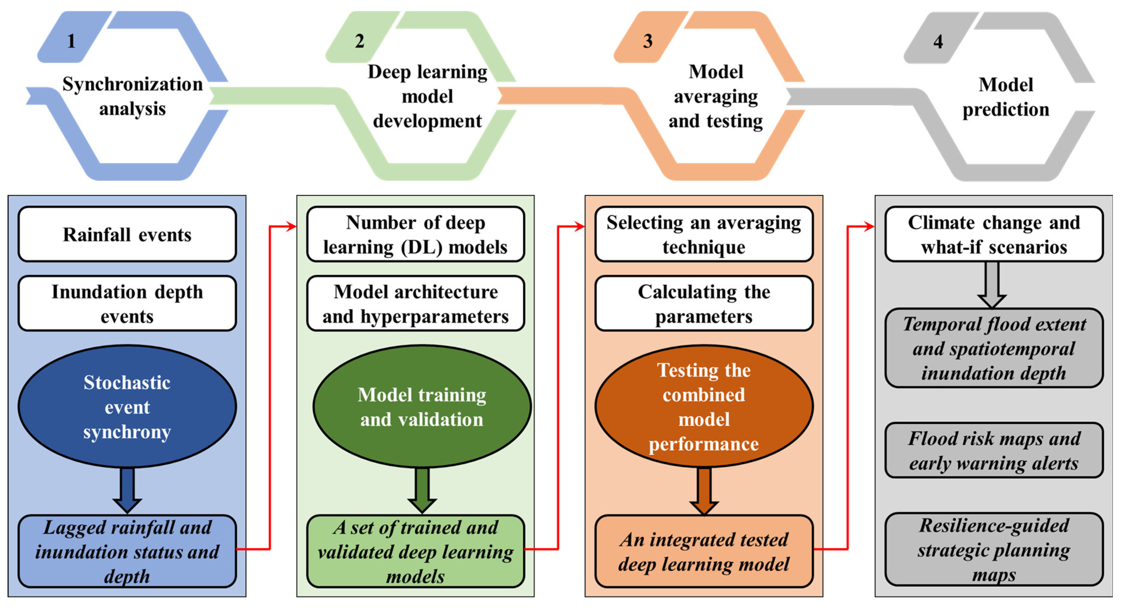
The FPM shown in Figure 1 consists of four modules: (1) a synchronization module, where the lagged interdependence between rainfall (i.e., input) and inundation depth (i.e., output) is quantified and the corresponding input-output pairs are identified; (2) a DL module, in which a set of candidate models with similar or different architectures are trained and validated based on the input-output pairs identified in the previous module; (3) an averaging and testing module, where candidate models are combined into a single one that is subsequently tested using an independent (i.e., new) dataset; and (4) a prediction module, in which the integrated model developed in the previous module is used for estimating temporal maps of flood extent, inundation depth, and flood risk under climate change projections and for different what-if scenarios. Detailed descriptions of these four modules are provided in the following sections.
2.1. Synchronization Module
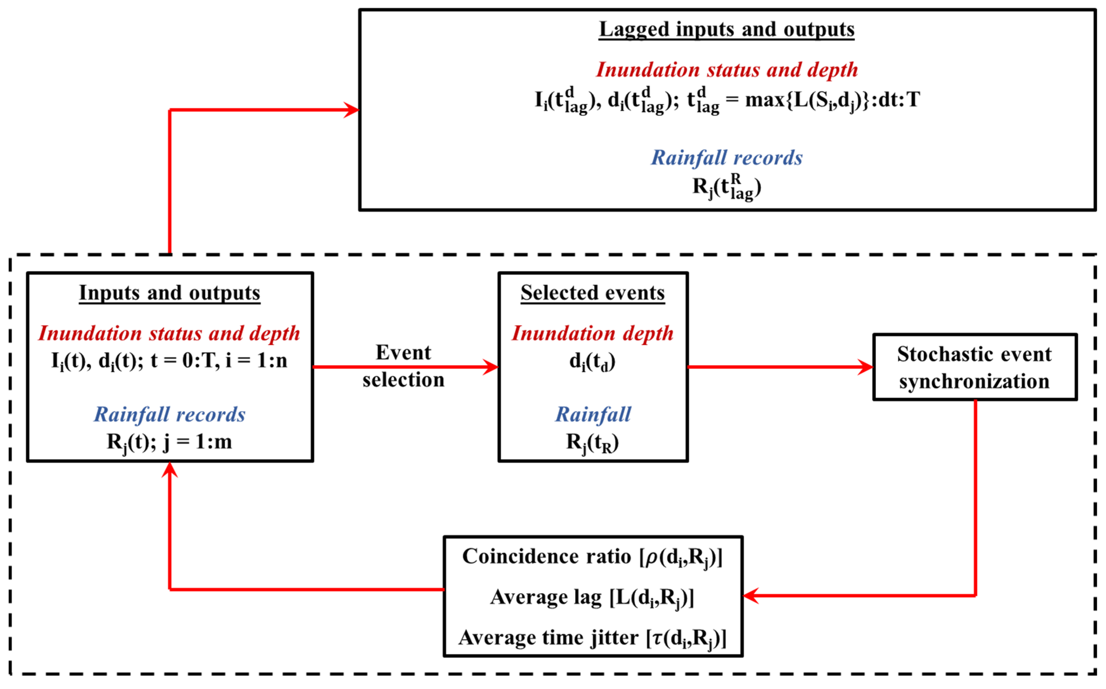
Coupled dynamic processes typically exhibit temporal correlation that reflects the interdependence between underlying systems [60]. This temporal correlation is known as synchronization [61], and can be quantified using linear and nonlinear metrics (e.g., cross-correlation, phase synchronization, coherence function, mutual information, event synchrony, and stochastic event synchrony) [62]. Some of these metrics (i.e., cross-correlation, phase synchronization, coherence function) are deterministic by nature; therefore, they most often fail to describe the synchronization between dynamic processes that are stochastic in nature (e.g., rainfall-flood, climate change-rainfall pattern). Probabilistic synchronization measures (e.g., mutual information, stochastic event synchrony) have thus been developed to overcome the limitations of their deterministic counterparts. The synchronization module (Figure 2) of the FPM employs the stochastic event synchronization (SES) approach to evaluate the lagged interdependence between rainfall and inundation depth, and subsequently develop a dataset of associated rainfall-depth pairs.
Assuming that and are the rainfall at weather station j at time t and inundation depth at location I at the same time, respectively, where Nt is the size of the set [t1:Δt:T], t1 is the initial recording time, Δt is the time step at which both rainfall and inundation depth are recorded, T is the maximum recording time, Nj is the number of weather stations employed, and Ni is the number of locations where inundation depth observations are available. and represent lagged, yet related, metrics characterizing the flood events under consideration. As such, for fluvial flooding conditions, records assume that urban drainage systems do not exist (or completely malfunction) in the study area. In contrast, the capacity and operability of drainage systems and other flood control measures are inherently present within records under pluvial or combined fluvial-pluvial flooding conditions. It should be noted that records can be acquired from a flood monitoring station at location i or can represent the output of a well-calibrated hydraulic or hydrologic-hydraulic model at such location. It should be also noted that when the timeseries of rainfall and inundation depth do not have the same Δt, a data imputation method should be applied. The application of SES starts with selecting peak rainfall [Rj(tR)] and inundation depth [di(td)] events from Rj(t) and di(t), respectively, with tR and td being the peak times of rainfall and inundation depth, respectively. It should be noted that other events may be selected (e.g., minimum or specific quantile values) depending on the study objective [63]. For instance, zero rainfall events may be employed to associate dry periods to drought occurrence, whereas a specified percentile of inundated areas may be related to poor dam operation conditions. Events selected from the two series (i.e., [Rj(tR)] and [di(td)]) are subsequently aligned such that a rainfall event at time tR is associated with a depth event between tR − δ and tR + δ, where δ is a pre-defined time window [62]. In contrast to the event synchronization approach developed by Quiroga et al., 2002 [62] that evaluates the synchronization between two timeseries based on reliability only, the SES quantifies both the reliability and precision aspects of synchronization [64]. Within the SES approach, the synchronization reliability is quantified through the coincidence ratio (ρ[di,Rj]) that indicates the fraction of events paired at a specific time lag ts.
As the collection of paired events may not be exactly lagged by ts, an average time lag [L(di,Rj)] is selected as the optimal lag and an average time jitter [τ(di,Rj)] is utilized to reflect the synchronization precision (i.e., the average deviation between ts and L). Rainfall amounts at station j is thus synchronized with inundation depths at location i at L(di,Rj) when ρ(di,Rj) is sufficiently high and τ(di,Rj) is notably low. It should be emphasized that the fact of causality between rainfall and flooding leads the rainfall events to always precedes inundation depth events. As such, negative L(di,Rj) values indicates that while j and i may be within the same hydrological system, the two locations are hydraulically disconnected and therefore rainfall-depth synchronization cannot be confirmed even for high values of ρ[di,Rj]. It should be also noted that while higher ρ(di,Rj) values reveal the synchronization between rainfall and depth processes at locations i and j, such synchronization should be physically confirmed as locations i and j may not be hydraulically connected in nature.
Once the synchronization is confirmed between Rj(tR) and di(td) pairs, an integrated database of lagged rainfall records , inundation depth values , and flooding status is prepared as shown in Figure 2, where , NL is the length of the vector , , and is the rainfall records (i.e., [Rj(t)]) shifted by time lags in the set . It should be highlighted that both of and represent the output of the deep learning model whereas is used as the model input. It should also be emphasized that the synchronization analysis module of the FPM can be used on its own as an early flood warning system as L(di,Rj) can reflect the time at which a peak inundation depth occurs at location i shortly after observing a peak rainfall event at weather station j, given that locations i and j are within the same hydraulic system. However, when synchronization is mathematically confirmed between rainfall and inundation depth at locations i and j that are within the same hydrologic system but are hydraulically disconnected, a homogenous rainfall regime can be suggested within the system (i.e., rainfall patterns, rather that intensities, are nearly the same over the watershed). Such information can guide the decisionmakers to devise prompt preparedness, mitigation, and evacuation plans prior to the occurrence of a flood event, which can boost community resilience under such type of hazard. It should be noted that the synchronization module described herein is considered a preprocessing step within the FPM through which the number of rainfall days required to estimate the flood characteristics is determined.
2.2. Deep Learning Module
CNNs are supervised feed-forward DL tools that were originally developed to solve image classification and computer vision problems [58,65], and their application has recently been extended to hydrological and hydraulic modelling [52,54,57,58], autonomous driving [66,67], and diagnosing chronic diseases [68,69]. A typical CNN consists of an input layer of 2D images with multiple channels, one or more convolution kernels that utilize a number of filters (Nf) to convert the input images into feature maps with reduced dimensions, nonlinear function (e.g., sigmoid function or rectified linear unit) to constraint the pixel values within the feature maps to a specific range, sub-sampling (i.e., pooling) layer to spatially integrate distinct pixels of each feature map, and an output layer [65]. The convolution kernel and nonlinear function together with the subsampling layer are referred to as the convolution layer (CL). A convolution block (CB) of multiple CLs connected in series, as shown in Figure 3, introduce more trainable parameters to the network to effectively explore complex input-output relationships [65]. However, the training of CNNs with several connected CBs may be computationally expensive [65], most often results in only locally optimized trainable parameters [70], and increases the likelihood of overfitting [71,72]. Enhanced performance can be achieved through employing a batch normalization directly after applying the convolution kernels and/or a dropout layer following the subsampling layer [53,73]. It should be highlighted that CNNs can integrate the spatial information within individual 2D images that are temporally related without capturing the time-interdependence between them.
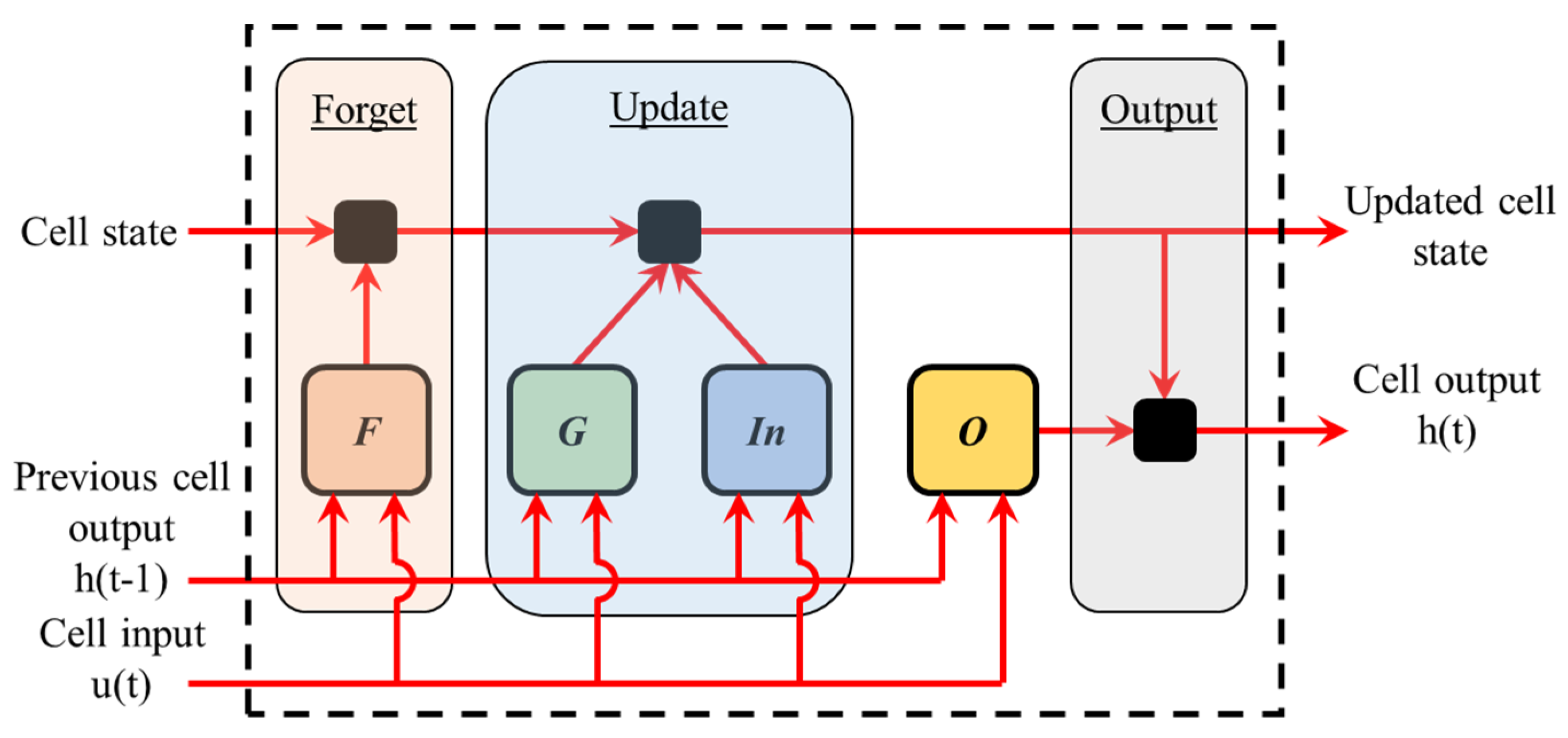
The LSTM network is a class of recurrent neural networks that can store, update, and modify information from interrelated consecutive sequences of temporally varying features through memory blocks [74]. Such information is subsequently combined to identify the relationship between the network inputs and outputs. LSTM networks employ a set of hidden units, each has a forget (F), candidate (G), input (In), and output (O) gate. The input of each hidden unit at a certain time step, u(t), is combined with its output from the previous one, h(t − 1), and are together fed to each of the four gates, as shown in Figure 4. Subsequently, the forget gate determines the amount of information to be omitted, the candidate gate identifies the important information to be memorized, the input gate introduces updating information to the hidden unit, and the output gate is utilized to combine u(t) and h(t − 1) with the long-term memory stored in the cell (i.e., cell state). The cell state is subsequently updated based on that stored previously after integration with the outputs from the forget, candidate, and input gates.
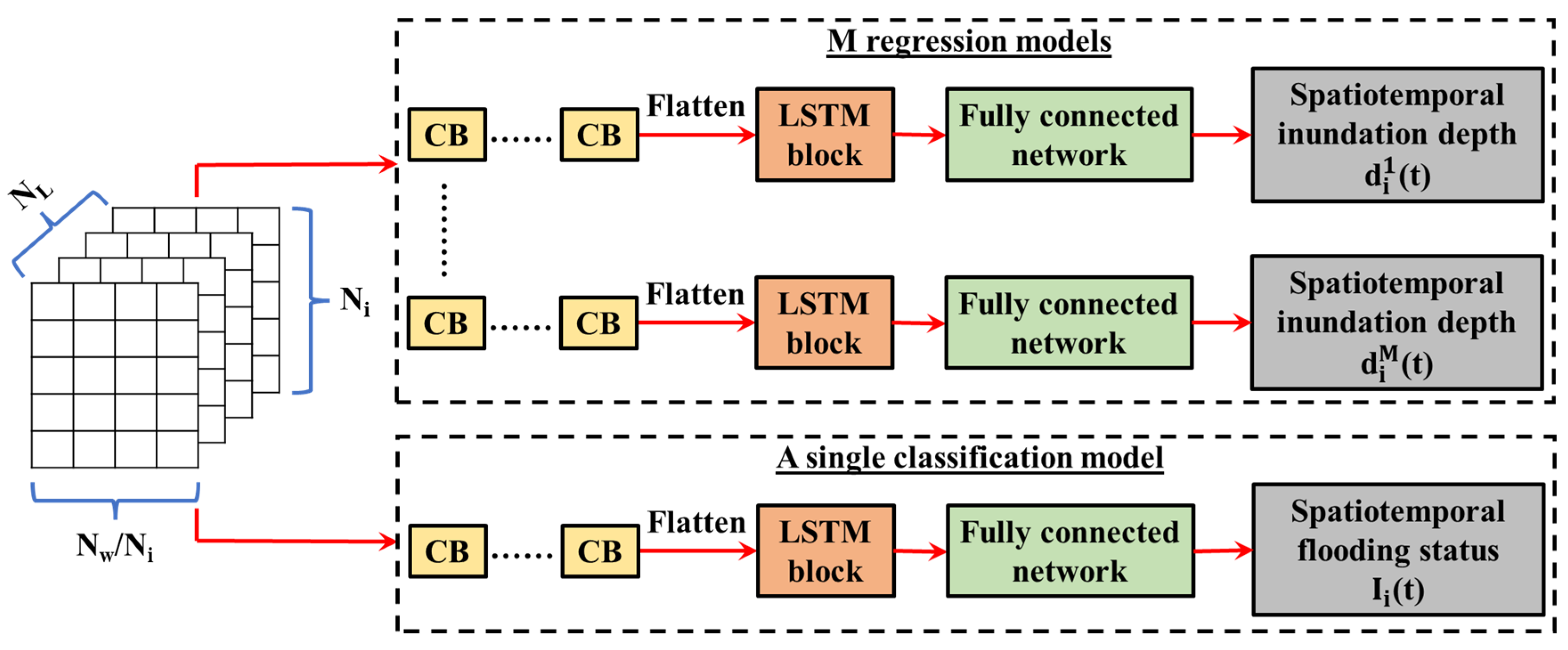
Due to the ability of CNN to integrate the spatial information within 2D datasets into meaningful features and the efficiency of LSTM network to capture the long-term temporal interdependence within a sequence, this module of the FPM combines both techniques. Accordingly, is reformulated as a number of NL 2D images, each with entries , and are subsequently used to train a M + 1 set of parallelly connected DL models (of which M are regression models used for inundation depth estimation and a single classification model utilized for flood extent prediction). Such reformulation implies that the DL models are used to estimate the flood extent and the spatial distribution of inundation depth at a specified time t due to a rainfall sequence within the time interval . In addition, estimating the flood extent is conceptualized as a classification problem, where locations are labelled as flooded/unflooded. Each of the DL models within this module consists of a number of CBs connected in series, followed by a LSTM network with Nh hidden unites. As the typical output from a CB is a 2D image, a flatten layer is added between the last CB and the LSTM network to collapse the spatial dimension of such images (i.e., converting 2D datasets into vectors). Finally, a fully connected network is used to map the output from the LSTM network into the output of interest (i.e., inundation depth or flooding status). Figure 5 shows a schematic of the DL module of the FPM. It should be noted that model parameters of such coupled CNN-LSTM architecture include values within each convolution kernel, weights and biases associated with inputs of each cell within the LSTM block, and neuron’s weights and biases in the fully connected network. Such parameters are typically obtained following a feedforward backpropagation optimization procedure (e.g., stochastic gradient descent [75] or adaptive moment estimation [76] approaches).
2.3. Averaging and Testing Module
The development of data-driven models, particularly those based on DL, necessitates using a massive number of input-output pairs to uncover complex relationships [77,78]. There is also a consensus that the model accuracy can be boosted significantly through increasing the size of the training dataset [79]. However, obtaining a large amount of data is challenging as only finite resources typically exist, and therefore the model parameters may not be optimized globally [80]. Several deterministic (e.g., simple model averaging, Granger–Ramanathan averaging, and artificial neural network) and probabilistic (i.e., Bayesian model averaging) multi-model ensemble approaches have therefore been suggested to combine forecasts from different models into more reliable predictions [81,82,83]. Of such approaches, the performance of the Bayesian model averaging (BMA) has been employed within different fields of the earth and planetary science including climatology [84,85,86], hydrology [87,88,89], and hydrogeology [90,91,92]. Therefore, the first step in this module of the FPM is to employ the BMA technique to combine the M spatiotemporal flood inundation predictions obtained from the DL module into a single estimate at each time t.
The application of the BMA relies on assigning a weight (Wm) to each candidate model m based on the corresponding contribution to the ensemble posterior distribution [93]. A normality assumption is typically employed, where estimates from each model m should follow a Gaussian distribution. Such assumption is most often violated, and thus model estimates should be transformed into Gaussian latent variables [83,94]. An expectation-maximization (EM) algorithm is subsequently applied with the objective of maximizing the following likelihood function:
where θ is the likelihood function with parameters Wm and σm, y|m is the estimates from model m after mapping into Gaussian space, and is the normal probability density of y using a mean value of y|m and a standard deviation of σm. In the context of this study, the BMA is applied to the M regression DL models only in order to produce highly reliable inundation depth maps at time t. Inundation depth estimates from the M regression models, , are therefore combined into using the Wm values obtained through the application of the EM algorithm to Equation (1), as follows:
The last step of this module is to test the performance of the regression and classification DL models using an independent set of rainfall sequences (i.e., different than those used for model training) such that their generalizability can be supported. The Nash-Sutcliffe efficiency (NSE) coefficient [95] is thus used to evaluate the performance of the BMA-based DL model, whereas the precision, recall, and F-score are used to assess that of the classification model [58]. The NSE coefficient is a model performance criterion that is typically less than or equal to 1.0 with values larger than 0.8 reflect higher model predictability and smaller prediction errors [96,97,98,99], and is quantified as:
where is the mean inundation depth across all Ni locations at time t. On the other hand, for classification models, the precision is defined as the fraction of accurately classified instances among the total estimates of a specific class (i.e., flooded/unflooded) [58]. The recall, in contrast, is the fraction of accurately classified instances among the total observations of a specific class. The precision and recall thus reflect the ability of a classification model to accurately predict the different classes, albeit from different perspectives [58]. Therefore, there is a consensus to combine both metrics harmonically into a F-score, where higher values indicate the significant predictability of the classification model (i.e., the model’s ability to estimate the flood extent for a sequence of rainfall events, in the context of the present study). It should be reminded that a single prediction of the classification and BMA-based DL models indicates the flood extent and the spatial distribution of inundation depth, respectively, at a specific instance of time t.
2.4. Prediction Module
The last module of the FPM provides hydrologists and decisionmakers with the ability to investigate the system response under expected (i.e., climate change projections) and hypothesized (i.e., what-if) flood scenarios. The results of this module’s analyses are flood extent, inundation depth, vulnerability, and risk maps. Such maps can guide future development and urban expansion plans, as well as flood mitigation and climate adaptation strategies. This can ultimately contribute to enhancing community resilience under extreme weather events, and specifically floods.
3. Study Area and Data Description
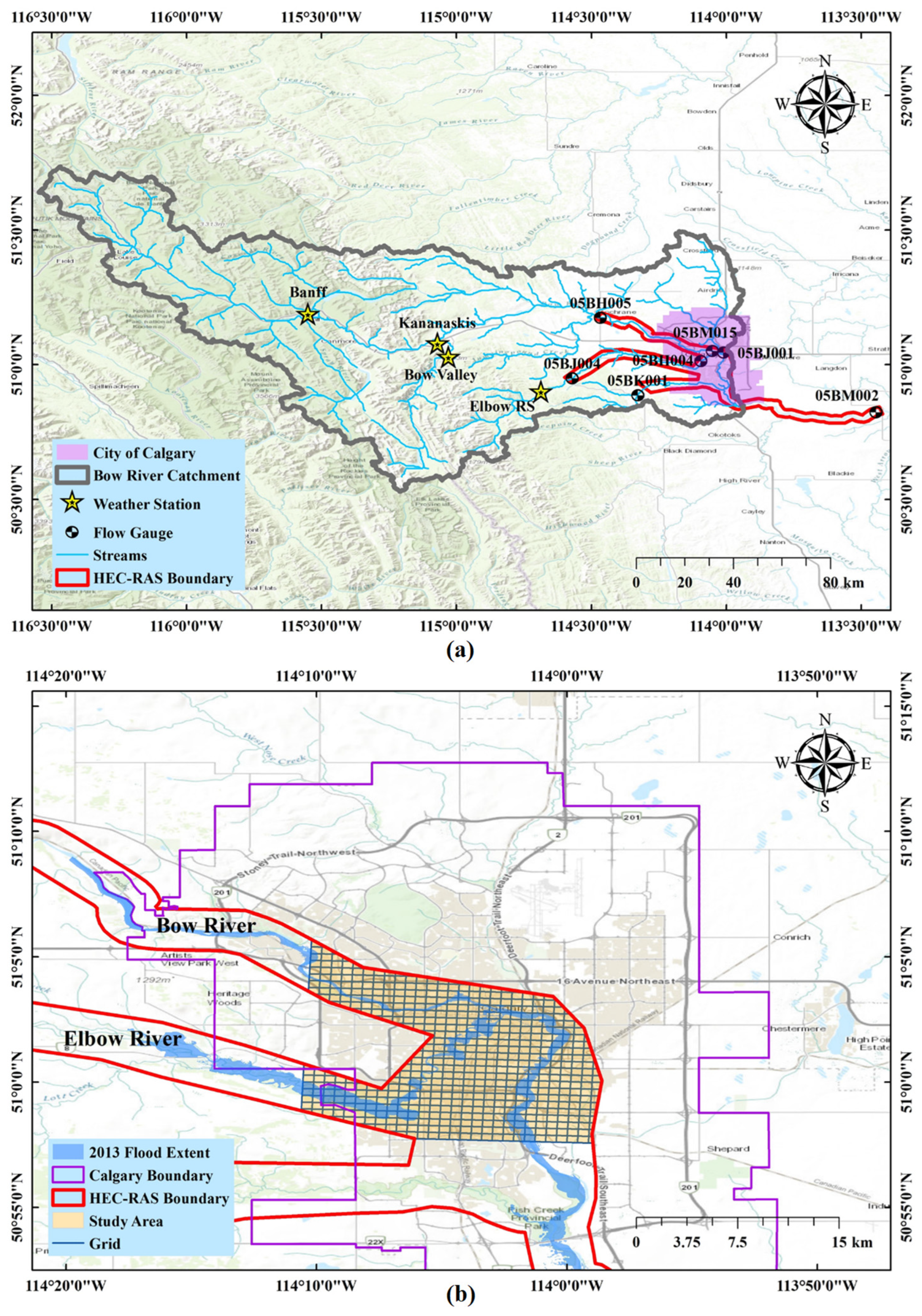
Calgary is among the largest three cities in Canada, with a population size and annual population increase of approximately 1.37 million and 0.66%, respectively (https://www.alberta.ca/ (accessed on 11 October 2022)). The City of Calgary locates within the Bow and Elbow catchment in the southwestern part of the province of Alberta, and is bounded by the Rocky Mountain Foothills to the west and the Canadian Prairies to the east (Figure 6). Both Bow and Elbow rivers enter the city from its western boundary and merge at the downtown area. Calgary has an average high temperature of 17 °C in summer and average low temperature of −10 °C in winter, and is known for its seasonal flooding conditions from May to September with an average peak precipitation of approximately 100 mm/day. Although a large body of Calgary’s economy (i.e., cooperates and governmental agencies) locates within the flood vulnerably downtown area, there is no permanent mitigation plans. As such, the city has experienced a devastating flood event in 2013, which resulted in monetary losses of approximately 5 billion dollars and caused around 100,000 of people to flee their homes. A flood risk prediction tool is therefore key for the City of Calgary to estimate, be prepared to, and minimize expected flood-induced damages, and subsequently boosting the city resilience under future flood events.
As illustrated before in Figure 6, the City of Calgary is exposed to both the Bow and Elbow catchments that have a collective area of about 11,000 km2. Bow River contributes a higher flow compared to that of Elbow River as it has larger tributaries that covey more surface runoff volume. Two flow gauges, 05BH005 and 05BJ004, locate at the city entrance on Bow and Elbow Rivers, respectively, as shown in Figure 6a. Such gauges provide flow measurements between March and October only when the river is not frozen. Flow records from 2010 to 2015 and from 2018 to 2020 at 05BH005 and 05BJ004 are obtained from the City of Calgary’s Open Data Portal (https://data.calgary.ca/ (accessed on 25 April 2022)). It is also noteworthy that flow records in 2016 and 2017 are not available at 05BH005 and 05BJ004 due to gauge maintenance. Available flow records are employed within the calibrated HEC-RAS model developed by Ghaith et al. [24] for the same study area to estimate actual flood extent and inundation depth maps during the aforementioned time intervals (referred to as observations hereafter). In contrast to the 1D/2D modelling approach that rely on representing the main rivers as 1D channels divided into multiple reaches with cross sections defined at different locations over the reaches, the 2D/3D hydraulic model developed by Ghaith et al. [24] adopts a 2D grid with 250 m square cells to overlay the study area (similar to that shown in Figure 6b). Such grid was subsequently partitioned into two regions, with the corresponding Manning’s roughness coefficients being calibrated based on the inundation depth measured at stations 05BM015, 05BJ001, and 05BH004 (Figure 6a) in 2013 as well as the maximum flood extent. Upstream boundary conditions were represented by flow measurements at stations 05BH001, 05BJ004, and 05BK001, whereas a normal depth based on the ground slope was assumed as the downstream boundary condition at station 05BM002 (Figure 6a). While HEC-RAS models do not intrinsically consider the interactions between fluvial and pluvial flood conditions as well as the capacity and operability of man-made flood control measures (e.g., basement spaces, drainage systems, flood protection structures), model calibration based on locations within both the river and overland flow areas enables capturing such interactions. Thus, fluvial flooding conditions are only assumed in this demonstration as all stations used by Ghaith et al. [24] for model calibration (i.e., 05BM015, 05BJ001, and 05BH004) locate within the rivers as shown in Figure 6a. It should be noted that actual flood extent and depths can be alternatively acquired through either spatially interpolating observations from a dense flood monitoring network or processing satellite images for the study area over time. However, such approaches are not applied in this FPM demonstration study due to data limitations. As the application of the FPM requires rainfall records and corresponding flood extent and inundation depths, four weather stations (Banff, Bow Valley, and Kananaskis stations on Bow River, and Elbow Ranger Station on Elbow River) are selected as shown in Figure 6a. These stations contain daily rainfall records which are acquired from the open portal of the province of Alberta (https://www.alberta.ca/ (accessed on 25 April 2022)). A study area is selected within the City of Calgary to demonstrate the utility of the FPM, and is subsequently divided into a mesh of 500 m × 500 m grid cells. Rainfall records at the four weather stations and corresponding flood hazard (i.e., extent and depth) maps over the selected study area are divided into training (from 2010 to 2015) and testing (from 2018 to 2020) subsets. Rainfall-flood characteristics pairs in the training interval were used within the first two modules of the FPM for input-output preparation and DL model development, whereas those in the testing interval were used for model testing within the third module. It should be highlighted that while a smaller cell size (i.e., 250 m × 250 m) was used within the hydraulic model developed by Ghaith et al. [24], larger grid cells are used when the FPM is applied for demonstration purposes only. It should be also noted that finer grids can be utilized to capture the flood characteristics at higher spatial resolutions (e.g., at the building scale); however, this could be associated with exorbitant computational costs. Thus, when the FPM is applied based on outputs from a hydrodynamic model, a sensitivity analysis should be carried out during the model development stage to evaluate the impact of cell size on the stability of numerical simulations as well as its suitability for flood resilience assessment and mapping purposes. Alternatively, when the FPM is applied using ground-truth observations from a flood monitoring network with sufficient control locations, spatial interpolation techniques can be used to calculate corresponding observations at the required resolution. It should be also noted that the Bow and Elbow rivers are distinct hydraulic systems that are supplied by different tributaries. However, the two rivers are joined near the City of Calgary’s downtown, forming a single flow route beyond their confluence. As a result, rainfall recorded at weather stations on the Bow river’s tributaries (i.e., Banff, Bow Valley, and Kananaskis) do not contribute to the discharge in the Elbow River at locations upstream the confluence of the two rivers. Similarly, weather stations on the Elbow river’s tributaries (i.e., Elbow Ranger Station) are not hydraulically connected to locations on the Bow River upstream the confluence of the two rivers.
4. Results and Discussion
4.1. Synchronization Analysis Results
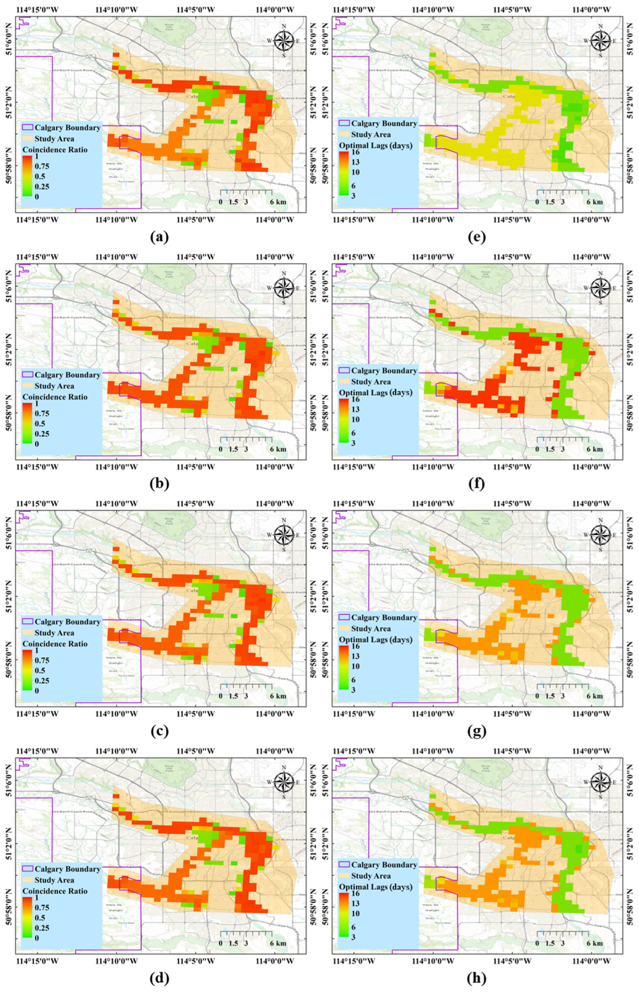
Figure 7 shows the results of the synchronization module in terms of the coincidence ratio ρ[di,Rj] and the optimal time lag L[di,Rj] using the rainfall records from the weather stations shown in Figure 6a and inundation depth values observed at the center of grid cells shown in Figure 6b between 2010 and 2015. The high ρ[di,Rj] values at the majority of cells, as shown in Figure 7a–d, highlight the synchronization between the rainfall records and inundation depth at the different grid cells at the corresponding optimal lags (Figure 7e–h). Even though some of the employed weather stations are not connected hydraulically to grid cells within different parts of the system as described earlier, the synchronization analysis results presented in Figure 7 support that respective rainfall observations and inundation depth estimates can still be related mathematically rather than physically. The L[di,Rj] values range between 3 to 16 days and are consistently smaller within the Bow River compared to those within the Elbow River, highlighting the higher water velocity in the former. In addition, the nearly constant L[di,Rj] values within both river basins suggest the lower routing effect and the consistent strength of propagating flood waves in both basins. These results support the utility of the synchronization analysis module of the FPM as a stand-alone flood warning system that can be used to estimate the lead time between peak rainfall occurrence and flood realization.
4.2. Deep Learning Model Development and Performance Evaluation
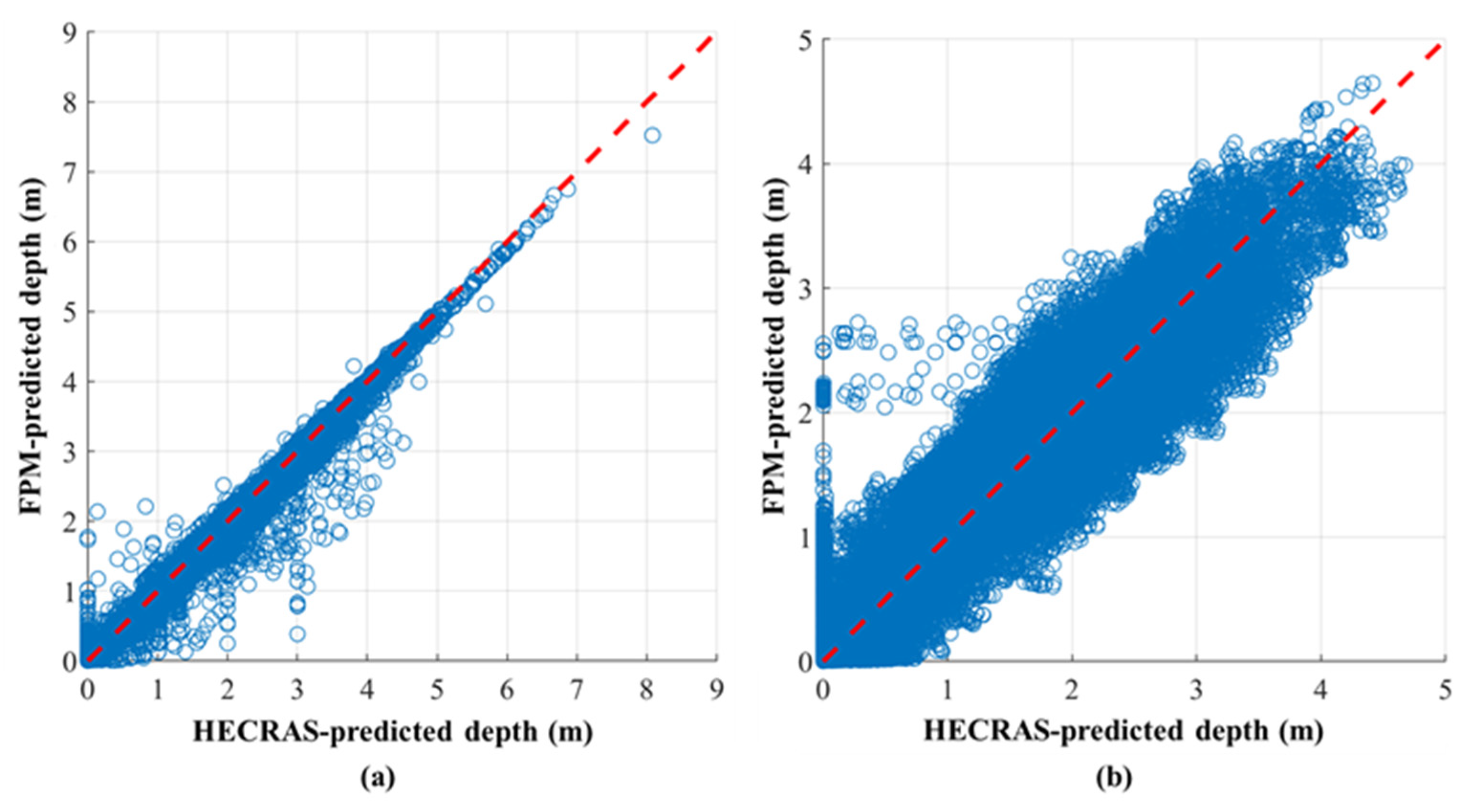
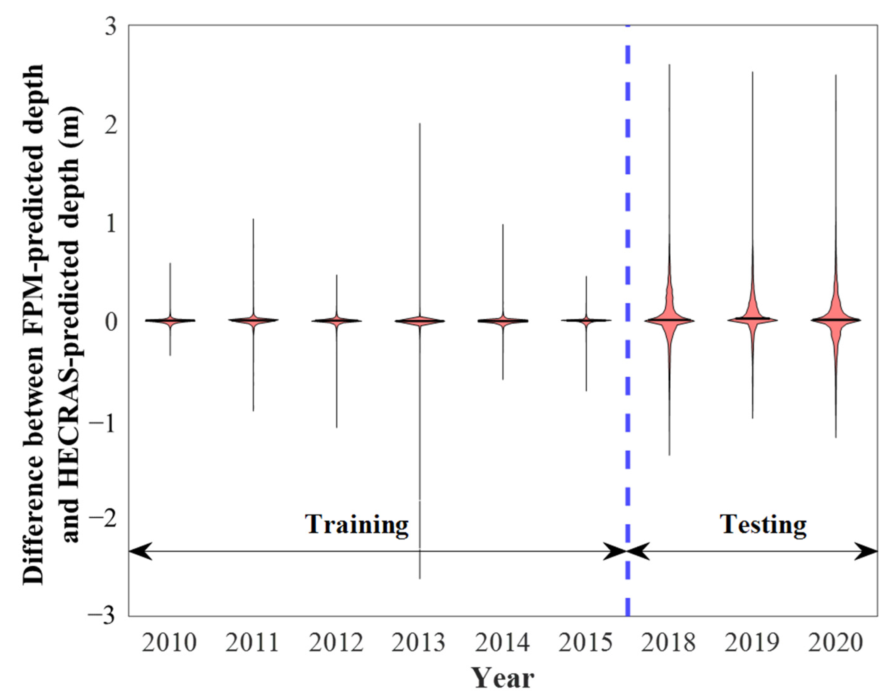
The optimal time lags (i.e., L[di,Rj]) shown in Figure 7 are subsequently employed for the preparation of the DL model inputs and outputs in the training and testing intervals as described in the DL module section (i.e., rainfall events in days t − 16 through t − 3 are used to estimate flood characteristics in day t). Rainfall records at the Banff, Bow Valley, Elbow Ranger, and Kananaskis stations between 2010 and 2015 (1362 instances) were used for model training, whereas corresponding records between 2018 and 2020 (681 instances) were used for model testing. Such records were reformulated as described in the Materials and Methods Section and classification- and BMA-based DL models are subsequently developed. Both models could efficiently replicate the flood extent (Table 1) and inundation depth (Figure 8) observations at most of the time instances in both the training and testing intervals. For the classification model, the overall precision, recall, and F-score were higher than 95% during approximately 99% and 96% of the time instances in the training and testing intervals, respectively. Grid cells overlaying the river (shown in Figure 6b) were falsely classified as flooded/unflooded less than 6% and 10% during the training and testing intervals, respectively, whereas those within overland flow areas were falsely classified around 9% and 5% within the training and testing intervals, respectively. In addition, F-score was consistently higher for locations within the river boundaries during both the training and testing intervals as shown in Table 1. This highlights the ability of the FPM to accurately allocate flooded and unflooded cells, and therefore inferring the flood extent. For the BMA-based model, 240 candidate DL models were trained and subsequently weighted using the BMA technique as described earlier. All of the candidate models efficiently reproduced the flood depth observations with average NSE values ranging between 0.84 and 0.97 and between 0.61 and 0.88 for the training and testing intervals, respectively. Such average NSE values were calculated based on all grid cells and all time instances within the training and testing intervals. More specifically, the DL models replicated the flood depth estimates across all grid cells with a NSE value that is larger than 0.8 for more than 98% of the time instances within the training interval. Within the testing interval and based on all of the 240 DL models, the NSE values were larger than 0.8 for approximately 74% to 92% of the time instances. On the other hand, within the ensemble BMA model, only 25% of the candidate DL models (i.e., 60 models) have relatively higher BMA weights that range between 0.0041 and 0.15. In addition, the NSE values were higher than 0.8 for approximately 99% and 92% of the time instances in the training and testing intervals, respectively, with most of the errors are less than 1.0 m (approximately 99% of the training errors and 94% of the testing errors are within ±0.5 m) as shown in Figure 9. For grid cells overlaying the river, the 95th percentile of depth prediction errors was 0.07 m and 0.61 m for the training and testing intervals, respectively. The same measure was 0.05 m and 0.41 m in overland flow areas during the training and testing intervals, respectively. Such results support the capability of the FPM to accurately predict the spatial distribution of inundation depth due to fluvial floods at different instances of time within both the training and testing intervals. It should be emphasized that the use of the FPM to predict the flood extent and inundation depth over a single year is 200 times faster than using a corresponding HEC-RAS model (i.e., computational time of using the FPM is 0.5% less that of using HEC-RAS).
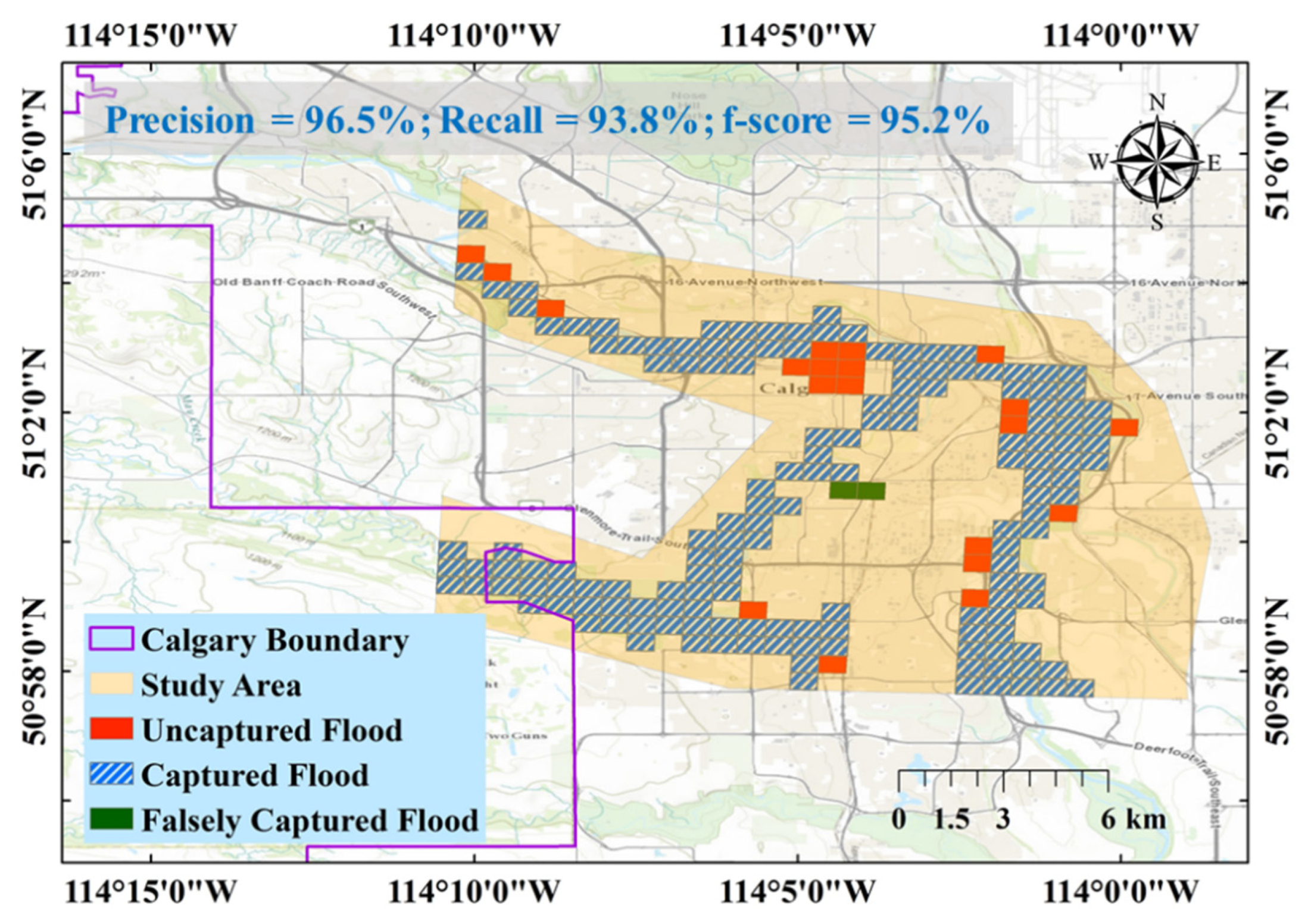
4.3. Example of Model Predictions
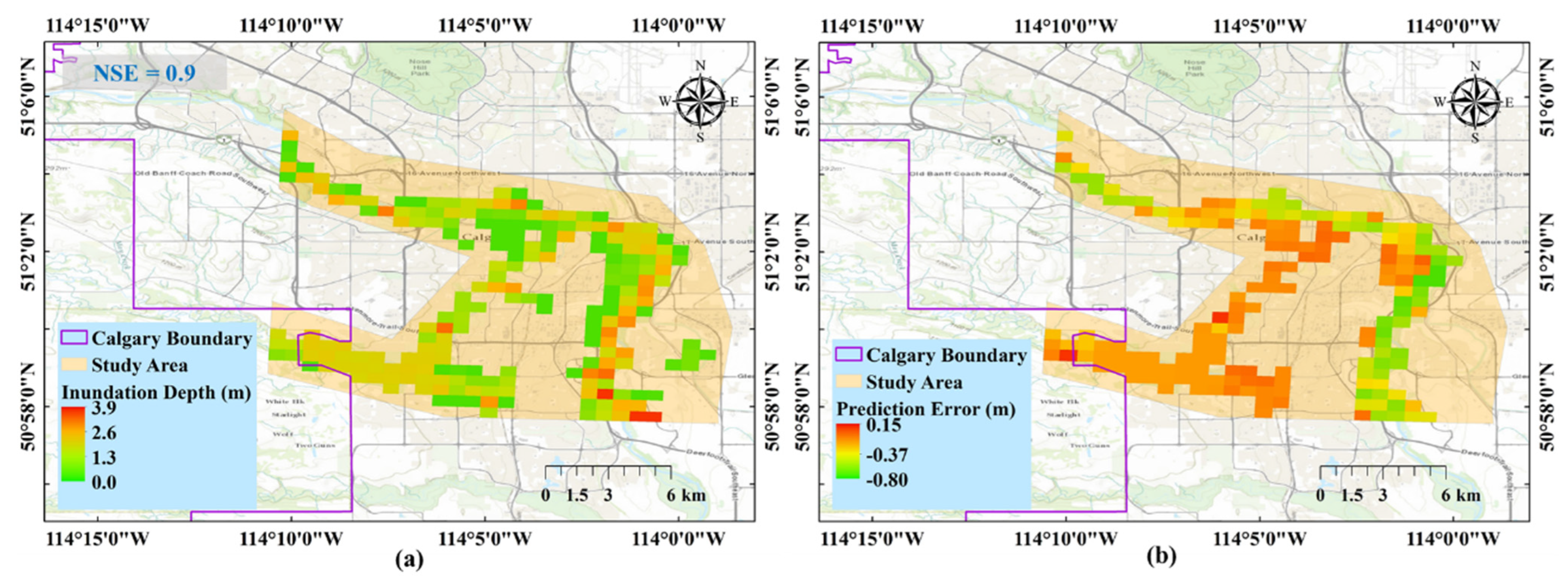
To further support the utility of using the FPM for flood hazard prediction in the City of Calgary, Figure 10 and Figure 11 show, respectively, the flood extent and inundation depth (and associated prediction errors) on 3 July 2020 (i.e., within the testing interval). The classification-based DL model efficiently reproduced the actual flood extent with F-score of 95.2%, reflecting a misclassification error of less than 5%. As shown in Figure 10, misclassified cells are within the overland flow areas where flooding occurs less frequently (i.e., lower water depths are recorded at such locations as shown in Figure 11a). For the inundation depth, the BMA-based DL model replicated the corresponding observations with a NSE value of 0.9 and a maximum error of less than 0.8 m. Small prediction errors are observed in both the Bow and Elbow rivers upstream their confluence (within both the river boundaries and overland flow areas), and are associated with shallower water depths. In contrast, large errors are encountered within the river boundaries downstream the confluence of the two rivers where water depths are large. It should be also highlighted that errors in inundation depth predictions shown in Figure 9 and Figure 11 are estimated as the difference between and the HECRAS-predicted depths at the same instance of time t. Therefore, positive- and negative error values indicate that the FPM overestimates and underestimates the inundation depth, respectively.
5. Insights for City Digital Twin Development and Climate Resilience Planning
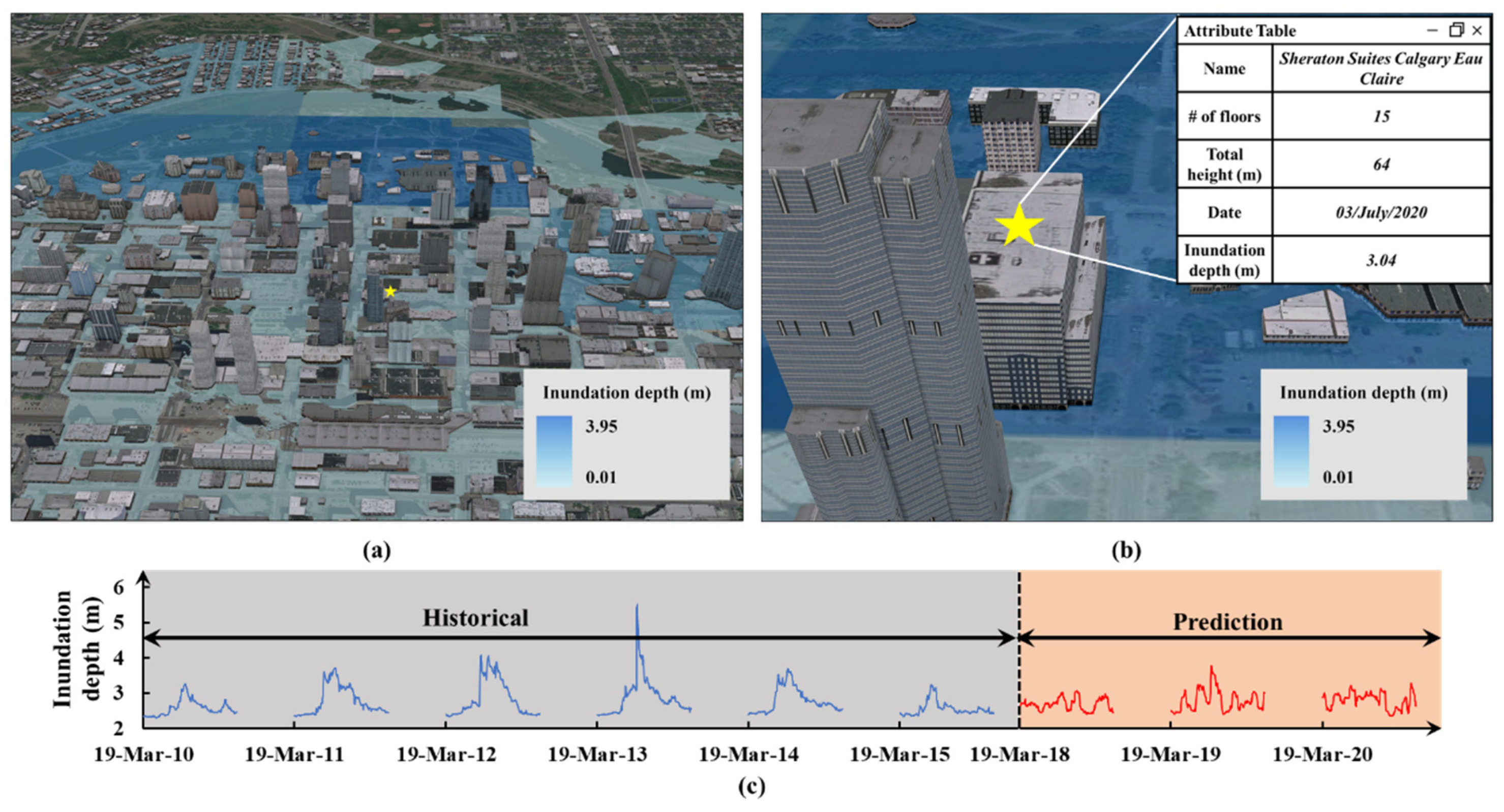
The FPM developed in this study represents a computationally efficient and accurate flood hazard prediction tool that can be easily integrated with models simulating other physical phenomena in a CDT to provide early estimation of the extreme weather impacts on buildings and infrastructures. For example, as shown in Figure 12a, the FPM can provide the CDT (fed by rainfall sensor data and containing 3D building and infrastructure information) with the inundation maps, enabling the visual evaluation of fluvial flood impacts on existing as well as planned city physical systems. Flood impacts can be also evaluated for individual elements as shown in Figure 12b,c, given that the grid employed during the FPM application is properly sized for flood hazard mapping and climate resilience planning. Additional information (e.g., name, height, water depth at a specific time, and flood depth timeseries) can be accordingly obtained and investigated. A CDT can also be immediately provided with flood risk maps estimated using the FPM as well as the expected down time and damage cost due to a design or hypothesized flood event for resilience quantification purposes. It should be noted that while the applicability of the FPM may be restricted to the range of rainfall and inundation depths used for model training, future developments causing a drastic change in land use, infrastructures, man-made flood control structures, and land cover can be accommodated within the FPM through a retraining process. This is nonetheless considerably faster and more reliable than developing new hydrologic and hydraulic models that are typically calibrated separately. However, it should be emphasized that while physics-based hydrologic and hydraulic models can be used within a CDT, the use of the FPM is proposed in this study to accelerate the computational procedures (from hours/days when using the hydrologic and hydraulic models to seconds/minutes when using the FPM). Decision- and policymakers can thus promptly devise action plans, mitigation and adaptation strategies, and resilience-enhancement methodologies to combat the flood impacts and other ongoing and expected climate change consequences.
6. Conclusions
In this study, a rapid data-driven early flood prediction methodology (FFM) is developed to replace the computationally expensive hydrological-hydraulic modelling processes typically used for flood hazard quantification. The FPM encompasses synchronization, deep learning (DL), averaging and testing, and prediction modules. The four modules are structured to facilitate the association between highly interdependent input-output pairs and boosting the prediction accuracy without the burden of the underlying complex physical processes. In the first module, the stochastic event synchronization approach is applied to evaluate the optimal time lag between peak rainfall and peak inundation depth events (reflecting fluvial, pluvial, or combined flooding conditions), and subsequently identify associated input-output pairs of rainfall sequences and flood characteristic (i.e., extent and depth). In the second module, a convolutional neural network (CNN) and long-short-term memory (LSTM) network are integrated in a feed-forward DL model to explore the complex, nonlinear relationship between the rainfall sequence and corresponding flood extent and inundation depth maps. As DL models may experience the phenomenon of overfitting and may not converge to a global optimal solution when the number of training instances is significantly small, the third module in the FPM consists of two parts: (1) applying a Bayesian model averaging (BMA) approach to combine estimates from different CNN-LSTM models such that the prediction errors are reduced and uncertainties in the model parameters are considered; and, (2) testing the ability of the BMA-based DL model to predict new output sets. The last module in the FPM aims at using the developed model to estimate flood hazard for an expected (i.e., climate change projection) or synthetic (i.e., what-if) scenario. To demonstrate its utility, the FPM was employed to simulate the rainfall-flooding process in the City of Calgary, Canada, considering only fluvial flooding conditions. In this respect, DL models were trained within the FPM using rainfall and inundation depth records from 2010 to 2015. After applying the BMA technique, the ability of the average model to predict the flood extent and inundation depth maps over 2018 to 2020 was evaluated. The FPM efficiently reproduced the flood hazard characteristics (with an efficiency of more than 95% for flood extent and more than 80% for inundation depth) estimated using a previously calibrated hydraulic (i.e., HEC-RAS) model for both the training and testing intervals. In addition, the application of the FPM requires less than 0.5% of the computation time required by the corresponding HEC-RAS model. The FPM is thus computationally superior, accurate, and ready-to-use tool—facilitating its integration as the computation core of a data-driven city digital twin (CDT). Such CDT can provide current and future insights for hydrologists, urban planners, decision- and policymakers, and land developers such that reliable early warning, preparedness, mitigation, and climate resilience strategies and plans can be promptly devised and tested.
Author Contributions
Conceptualization, methodology, formal analysis, investigation, writing—original draft preparation, M.G. and A.Y.; Conceptualization, writing—review and editing, supervision, project administration, funding acquisition, W.E.-D. All authors have read and agreed to the published version of the manuscript.
Funding
This research and the APC were funded by the Natural Sciences and Engineering Research Council of Canada (NSERC) through the Discovery Grant number [RGPIN-2021-03983].
Data Availability Statement
Data is contained within the article.
Acknowledgments
This research was supported by the Natural Sciences and Engineering Research Council of Canada (NSERC). Additional support from the Interdependent Network Visualization, Simulation, Optimization, Analysis, and Learning Laboratory (INViSiONLab) in McMaster University is gratefully acknowledged.
Conflicts of Interest
The authors declare no conflict of interest.
References
- McLennan, M. The Global Risks Report 2021: 16th Edition; World Economic Forum: Cologny, Switzerland, 2021. [Google Scholar]
- McLennan, M. The Global Risks Report 2022: 17th Edition; World Economic Forum: Cologny, Switzerland, 2022. [Google Scholar]
- Gaur, A.; Gaur, A.; Simonovic, S.P. Future Changes in Flood Hazards across Canada under a Changing Climate. Water 2018, 10, 1441. [Google Scholar] [CrossRef] [Green Version]
- Nofal, O.M.; van de Lindt, J.W. Understanding Flood Risk in the Context of Community Resilience Modeling for the Built Environment: Research Needs and Trends. Sustain. Resilient Infrastruct. 2020, 7, 171–187. [Google Scholar] [CrossRef]
- Gaur, A.; Gaur, A.; Simonovic, S.P. Modelling of Future Flood Risk across Canada Due to Climate Change. In WIT Transactions on Engineering Sciences; WIT Press: Southampton, UK, 2018; Volume 121, pp. 149–159. [Google Scholar]
- Tanaka, T.; Kiyohara, K.; Tachikawa, Y. Comparison of Fluvial and Pluvial Flood Risk Curves in Urban Cities Derived from a Large Ensemble Climate Simulation Dataset: A Case Study in Nagoya, Japan. J. Hydrol. 2020, 584, 124706. [Google Scholar] [CrossRef]
- UN Office for Disaster Risk Reduction. The Human Cost of Disasters—An Overview of the Last 20 Years 2000–2019; UN Office for Disaster Risk Reduction: Geneva, Switzerland, 2020. [Google Scholar]
- Tellman, B.; Sullivan, J.A.; Kuhn, C.; Kettner, A.J.; Doyle, C.S.; Brakenridge, G.R.; Erickson, T.A.; Slayback, D.A. Satellite Imaging Reveals Increased Proportion of Population Exposed to Floods. Nature 2021, 596, 80–86. [Google Scholar] [CrossRef] [PubMed]
- United Nations Office for Disaster Risk Reduction. 2020: The Non-COVID Year in Disasters; United Nations Office for Disaster Risk Reduction: Geneva, Switzerland, 2021. [Google Scholar]
- Pörtner, H.-O.; Roberts, D.C.; Adams, H.; Adelekan, I.; Adler, C.; Adrian, R.; Aldunce, P.; Ali, E.; Ara-Begum, R.; Bednar-Friedl, B.; et al. “Technical Summary” in Climate Change 2022: Impacts, Adaptation, and Vulnerability; Contribution of Working Group II to the Sixth Assessment Report of the Intergovernmental Panel on Climate Change; Cambridge University Press: Cambridge, UK, 2022. [Google Scholar]
- Ionita, M.; Nagavciuc, V. Extreme Floods in the Eastern Part of Europe: Large-Scale Drivers and Associated Impacts. Water 2021, 13, 1122. [Google Scholar] [CrossRef]
- CRED. Disasters in Africa: 20 Year Review 2000–2019; CRED: Bengaluru, India, 2019. [Google Scholar]
- Tembata, K.; Takeuchi, K. Floods and Exports: An Empirical Study on Natural Disaster Shocks in Southeast Asia. Econ. Disasters Clim. Chang. 2019, 3, 39–60. [Google Scholar] [CrossRef] [Green Version]
- Lin, H.; Mo, R.; Vitart, F.; Stan, C. Eastern Canada Flooding 2017 and Its Subseasonal Predictions. Atmosphere-Ocean 2019, 57, 195–207. [Google Scholar] [CrossRef] [Green Version]
- Kokas, T.; Simonovic, S.P.; Binns, A. Flood Risk Management in Canadian Urban Environments: A Comprehensive Framework for Water Resources Modeling and Decision-Making; Water Resources Research Report no. 095; Department of Civil and Environmental Engineering: London, ON, Canada, 2016. [Google Scholar]
- Neri, A.; Villarini, G.; Slater, L.J.; Napolitano, F. On the Statistical Attribution of the Frequency of Flood Events across the U.S. Midwest. Adv Water Resour 2019, 127, 225–236. [Google Scholar] [CrossRef]
- Billion-Dollar Weather and Climate Disasters. Available online: https://www.ncei.noaa.gov/access/billions/ (accessed on 20 March 2022).
- Sandink, D. Urban Flooding in Canada; Institute for Catastrophic Loss Reduction: Toronto, ON, Canada, 2013; Volume 52. [Google Scholar]
- Garner, A.J.; Mann, M.E.; Emanuel, K.A.; Kopp, R.E.; Lin, N.; Alley, R.B.; Horton, B.P.; DeConto, R.M.; Donnelly, J.P.; Pollard, D. Impact of Climate Change on New York City’s Coastal Flood Hazard: Increasing Flood Heights from the Preindustrial to 2300 CE. Proc. Natl. Acad. Sci. USA 2017, 114, 11861–11866. [Google Scholar] [CrossRef] [Green Version]
- Paprotny, D.; Vousdoukas, M.I.; Morales-Nápoles, O.; Jonkman, S.N.; Feyen, L. Compound Flood Potential in Europe. Hydrol. Earth Syst. Sci. Discuss. 2018, 132, 1–34. [Google Scholar] [CrossRef]
- Paprotny, D.; Sebastian, A.; Morales-Nápoles, O.; Jonkman, S.N. Trends in Flood Losses in Europe over the Past 150 Years. Nat. Commun. 2018, 9, 1985. [Google Scholar] [CrossRef] [Green Version]
- Berghuijs, W.R.; Aalbers, E.E.; Larsen, J.R.; Trancoso, R.; Woods, R.A. Recent Changes in Extreme Floods across Multiple Continents. Environ. Res. Lett. 2017, 12, 114035. [Google Scholar] [CrossRef]
- Schrotter, G.; Hürzeler, C. The Digital Twin of the City of Zurich for Urban Planning. PFG-J. Photogramm. Remote Sens. Geoinf. Sci. 2020, 88, 99–112. [Google Scholar] [CrossRef] [Green Version]
- Ghaith, M.; Yosri, A.; El-Dakhakhni, W. Digital Twin: A City-Scale Flood Imitation Framework. In Proceedings of the Canadian Society of Civil Engineering Annual Conference, Online, 26–29 May 2021; pp. 577–588. [Google Scholar] [CrossRef]
- Ruohomäki, T.; Airaksinen, E.; Huuska, P.; Kesäniemi, O.; Martikka, M.; Suomisto, J. Smart City Platform Enabling Digital Twin. In Proceedings of the International Conference on Intelligent Systems, Funchal, Portugal, 25–27 September 2018; pp. 155–161. [Google Scholar]
- Ivanov, S.; Nikolskaya, K.; Radchenko, G.; Sokolinsky, L.; Zymbler, M. Digital Twin of City: Concept Overview. In Proceedings of the Global Smart Industry Conference, Chelyabinsk, Russia, 17–19 November 2020; pp. 178–186. [Google Scholar]
- Ford, D.N.; Wolf, C.M. Smart Cities with Digital Twin Systems for Disaster Management. J. Manag. Eng. 2020, 36, 04020027. [Google Scholar] [CrossRef] [Green Version]
- Lu, Q.; Parlikad, A.K.; Woodall, P.; Don Ranasinghe, G.; Xie, X.; Liang, Z.; Konstantinou, E.; Heaton, J.; Schooling, J. Developing a Digital Twin at Building and City Levels: Case Study of West Cambridge Campus. J. Manag. Eng. 2020, 36, 05020004. [Google Scholar] [CrossRef]
- Abdel-Mooty, M.N.; Yosri, A.; El-Dakhakhni, W.; Coulibaly, P. Community Flood Resilience Categorization Framework. Int. J. Disaster Risk Reduct. 2021, 61, 102349. [Google Scholar] [CrossRef]
- Haggag, M.; Yosri, A.; El-Dakhakhni, W.; Hassini, E. Interpretable Data-Driven Model for Climate-Induced Disaster Damage Prediction: The First Step in Community Resilience Planning. Int. J. Disaster Risk Reduct. 2022, 73, 102884. [Google Scholar] [CrossRef]
- Ezzeldin, M.; El-Dakhakhni, W.E. Robustness of Ontario Power Network under Systemic Risks. Sustain. Resilient. Infrastruct. 2021, 6, 252–271. [Google Scholar] [CrossRef]
- Li, X.; Liu, H.; Wang, W.; Zheng, Y.; Lv, H.; Lv, Z. Big Data Analysis of the Internet of Things in the Digital Twins of Smart City Based on Deep Learning. Future Gener. Comput. Syst. 2022, 128, 167–177. [Google Scholar] [CrossRef]
- Papyshev, G.; Yarime, M. Exploring City Digital Twins as Policy Tools: A Task-Based Approach to Generating Synthetic Data on Urban Mobility. Data Policy 2021, 3, e16. [Google Scholar] [CrossRef]
- Lv, Z.; Xie, S. Artificial Intelligence in the Digital Twins: State of the Art, Challenges, and Future Research Topics. Digit. Twin 2021, 1, 12. [Google Scholar] [CrossRef]
- Austin, M.; Delgoshaei, P.; Coelho, M.; Heidarinejad, M. Architecting Smart City Digital Twins: Combined Semantic Model and Machine Learning Approach. J. Manag. Eng. 2020, 36, 04020026. [Google Scholar] [CrossRef]
- Dembski, F.; Wössner, U.; Letzgus, M.; Ruddat, M.; Yamu, C. Urban Digital Twins for Smart Cities and Citizens: The Case Study of Herrenberg, Germany. Sustainability 2020, 12, 2307. [Google Scholar] [CrossRef] [Green Version]
- National Research Foundation: Prime Minister’s Office: Virtual Singapore. Available online: https://www.nrf.gov.sg/ (accessed on 6 November 2022).
- Ham, Y.; Kim, J. Participatory Sensing and Digital Twin City: Updating Virtual City Models for Enhanced Risk-Informed Decision-Making. J. Manag. Eng. 2020, 36, 04020005. [Google Scholar] [CrossRef]
- Chomba, I.C.; Banda, K.E.; Winsemius, H.C.; Chomba, M.J.; Mataa, M.; Ngwenya, V.; Sichingabula, H.M.; Nyambe, I.A.; Ellender, B. A Review of Coupled Hydrologic-Hydraulic Models for Floodplain Assessments in Africa: Opportunities and Challenges for Floodplain Wetland Management. Hydrology 2021, 8, 44. [Google Scholar] [CrossRef]
- Bravo, J.M.; Allasia, D.; Paz, A.R.; Collischonn, W.; Tucci, C.E.M. Coupled Hydrologic-Hydraulic Modeling of the Upper Paraguay River Basin. J. Hydrol. Eng. 2012, 17, 635–646. [Google Scholar] [CrossRef]
- Clilverd, H.M.; Thompson, J.R.; Heppell, C.M.; Sayer, C.D.; Axmacher, J.C. Coupled Hydrological/Hydraulic Modelling of River Restoration Impacts and Floodplain Hydrodynamics. River Res. Appl. 2016, 32, 1927–1948. [Google Scholar] [CrossRef]
- Golmohammadi, G.; Prasher, S.; Madani, A.; Rudra, R. Evaluating Three Hydrological Distributed Watershed Models: MIKE-SHE, APEX, SWAT. Hydrology 2014, 1, 20–39. [Google Scholar] [CrossRef] [Green Version]
- Ghaith, M.; Li, Z. Propagation of Parameter Uncertainty in SWAT: A Probabilistic Forecasting Method Based on Polynomial Chaos Expansion and Machine Learning. J. Hydrol. 2020, 586, 124854. [Google Scholar] [CrossRef]
- Ghaith, M.; Li, Z.; Baetz, B.W. Uncertainty Analysis for Hydrological Models with Interdependent Parameters: An Improved Polynomial Chaos Expansion Approach. Water Resour. Res. 2021, 57, e2020WR029149. [Google Scholar] [CrossRef]
- Hosseiny, H. A Deep Learning Model for Predicting River Flood Depth and Extent. Environ. Model. Softw. 2021, 145, 105186. [Google Scholar] [CrossRef]
- Zanchetta, A.D.L.; Coulibaly, P. Hybrid Surrogate Model for Timely Prediction of Flash Flood Inundation Maps Caused by Rapid River Overflow. Forecasting 2022, 4, 126–148. [Google Scholar] [CrossRef]
- Gunathilake, M.B.; Karunanayake, C.; Gunathilake, A.S.; Marasingha, N.; Samarasinghe, J.T.; Bandara, I.M.; Rathnayake, U. Hydrological Models and Artificial Neural Networks (ANNs) to Simulate Streamflow in a Tropical Catchment of Sri Lanka. Appl. Comput. Intell. Soft Comput. 2021, 2021, 6683389. [Google Scholar] [CrossRef]
- Ghaith, M.; Siam, A.; Li, Z.; El-Dakhakhni, W. Hybrid Hydrological Data-Driven Approach for Daily Streamflow Forecasting. J. Hydrol. Eng. 2020, 25, 04019063. [Google Scholar] [CrossRef]
- Van, S.P.; Le, H.M.; Thanh, D.V.; Dang, T.D.; Loc, H.H.; Anh, D.T. Deep Learning Convolutional Neural Network in Rainfall-Runoff Modelling. J. Hydroinforma. 2020, 22, 541–561. [Google Scholar] [CrossRef] [Green Version]
- Baek, S.S.; Pyo, J.; Chun, J.A. Prediction of Water Level and Water Quality Using a Cnn-Lstm Combined Deep Learning Approach. Water 2020, 12, 3399. [Google Scholar] [CrossRef]
- Elmorsy, M.; El-Dakhakhni, W.; Zhao, B. Generalizable Permeability Prediction of Digital Porous Media via a Novel Multi-scale 3D Convolutional Neural Network. Water Resour. Res. 2022, 58, e2021WR031454. [Google Scholar] [CrossRef]
- Wang, Y.; Fang, Z.; Hong, H.; Peng, L. Flood Susceptibility Mapping Using Convolutional Neural Network Frameworks. J. Hydrol. 2020, 582, 124482. [Google Scholar] [CrossRef]
- Chang, D.L.; Yang, S.H.; Hsieh, S.L.; Wang, H.J.; Yeh, K.C. Artificial Intelligence Methodologies Applied to Prompt Pluvial Flood Estimation and Prediction. Water 2020, 12, 3552. [Google Scholar] [CrossRef]
- Chen, C.; Hui, Q.; Xie, W.; Wan, S.; Zhou, Y.; Pei, Q. Convolutional Neural Networks for Forecasting Flood Process in Internet-of-Things Enabled Smart City. Comput. Netw. 2021, 186, 107744. [Google Scholar] [CrossRef]
- Ghimire, S.; Yaseen, Z.M.; Farooque, A.A.; Deo, R.C.; Zhang, J.; Tao, X. Streamflow Prediction Using an Integrated Methodology Based on Convolutional Neural Network and Long Short-Term Memory Networks. Sci. Rep. 2021, 11, 17497. [Google Scholar] [CrossRef] [PubMed]
- Chen, C.; Jiang, J.; Liao, Z.; Zhou, Y.; Wang, H.; Pei, Q. A Short-Term Flood Prediction Based on Spatial Deep Learning Network: A Case Study for Xi County, China. J. Hydrol. 2022, 607, 127535. [Google Scholar] [CrossRef]
- Guo, Z.; Leitão, J.P.; Simões, N.E.; Moosavi, V. Data-Driven Flood Emulation: Speeding up Urban Flood Predictions by Deep Convolutional Neural Networks. J. Flood Risk. Manag. 2021, 14, e12684. [Google Scholar] [CrossRef]
- Kabir, S.; Patidar, S.; Xia, X.; Liang, Q.; Neal, J.; Pender, G. A Deep Convolutional Neural Network Model for Rapid Prediction of Fluvial Flood Inundation. J. Hydrol. 2020, 590, 125481. [Google Scholar] [CrossRef]
- Bentivoglio, R.; Isufi, E.; Nicolaas Jonkman, S.; Taormina, R. Deep Learning Methods for Flood Mapping: A Review of Existing Applications and Future Research Directions. Hydrol. Earth Syst. Sci. 2021, 614, 4345–4378. [Google Scholar] [CrossRef]
- Boccaletti, S.; Pisarchik, A.N.; del Genio, C.I.; Amann, A. Synchronization: From Coupled Systems to Complex Networks, 1st ed.; Cambridge University Press: Cambridge, UK, 2018; ISBN 978-1-107-05626-8. [Google Scholar]
- Boccaletti, S.; Kurths, J.; Osipov, G.; Valladares, D.L.; Zhou, C.S. Synchronization of Chaotic Systems. Phys. Rep. 2002, 366, 1–101. [Google Scholar] [CrossRef]
- Quiroga, R.Q.; Kreuz, T.; Grassberger, P. Event Synchronization: A Simple and Fast Method to Measure Synchronicity and Time Delay Patterns. Phys. Rev. E 2002, 66, 041904. [Google Scholar] [CrossRef] [Green Version]
- Yosri, A.; Dickson-Anderson, S.; Siam, A.; El-Dakhakhni, W. Transport Pathway Identification in Fractured Aquifers: A Stochastic Event Synchrony-Based Framework. Adv. Water Resour. 2021, 147, 103800. [Google Scholar] [CrossRef]
- Dauwels, J.; Vialatte, F.; Weber, T.; Musha, T.; Cichocki, A. Quantifying Statistical Interdependence by Message Passing on Graphs-Part I: One-Dimensional Point Processes. Neural. Comput. 2009, 21, 2152–2202. [Google Scholar] [CrossRef]
- Pelt, D.M.; Sethian, J.A. A Mixed-Scale Dense Convolutional Neural Network for Image Analysis. Proc. Natl. Acad. Sci. USA 2017, 115, 254–259. [Google Scholar] [CrossRef] [Green Version]
- Li, Y.; Yang, S.; Zheng, Y.; Lu, H. Improved Point-Voxel Region Convolutional Neural Network: 3D Object Detectors for Autonomous Driving. IEEE Trans. Intell. Transp. Syst. 2021, 23, 9311–9317. [Google Scholar] [CrossRef]
- Chen, S.; Leng, Y.; Labi, S. A Deep Learning Algorithm for Simulating Autonomous Driving Considering Prior Knowledge and Temporal Information. Comput.-Aided Civ. Infrastruct. Eng. 2020, 35, 305–321. [Google Scholar] [CrossRef]
- Rezk, E.; Eltorki, M.; El-Dakhakhni, W. Leveraging Artificial Intelligence to Improve the Diversity of Dermatological Skin Color Pathology: Protocol for an Algorithm Development and Validation Study. JMIR Res. Protoc. 2022, 11, e34896. [Google Scholar] [CrossRef]
- Muraki, R.; Teramoto, A.; Sugimoto, K.; Sugimoto, K.; Yamada, A.; Watanabe, E. Automated Detection Scheme for Acute Myocardial Infarction Using Convolutional Neural Network and Long Short-Term Memory. PLoS ONE 2022, 17, e0264002. [Google Scholar] [CrossRef]
- Krizhevsky, A.; Sutskever, I.; Hinton, G.E. ImageNet Classification with Deep Convolutional Neural Networks. In Advances in Neural Information Processing Systems; Pereira, F., Burges, C.J., Bottou, L., Weinberger, K.Q., Eds.; Curran Associates, Inc.: Red Hook, NY, USA, 2012; pp. 1097–1105. ISBN 9781627480031. [Google Scholar]
- Abdar, M.; Pourpanah, F.; Hussain, S.; Rezazadegan, D.; Liu, L.; Ghavamzadeh, M.; Fieguth, P.; Cao, X.; Khosravi, A.; Acharya, U.R.; et al. A Review of Uncertainty Quantification in Deep Learning: Techniques, Applications and Challenges. Inf. Fusion 2021, 76, 243–297. [Google Scholar] [CrossRef]
- Srivastava, N.; Hinton, G.; Krizhevsky, A.; Sutskever, I.; Salakhutdinov, R. Dropout: A Simple Way to Prevent Neural Networks from Overfitting. J. Mach. Learn. Res. 2014, 15, 1929–1958. [Google Scholar]
- Gao, M.; Chen, C.; Shi, J.; Lai, C.S.; Yang, Y.; Dong, Z. A Multiscale Recognition Method for the Optimization of Traffic Signs Using GMM and Category Quality Focal Loss. Sensors 2020, 20, 4850. [Google Scholar] [CrossRef]
- Fang, Z.; Wang, Y.; Peng, L.; Hong, H. Predicting Flood Susceptibility Using LSTM Neural Networks. J. Hydrol. 2021, 594, 125734. [Google Scholar] [CrossRef]
- Zhou, B.-C.; Han, C.-Y.; Guo, T.-D. Convergence of Stochastic Gradient Descent in Deep Neural Network. Acta Math. Appl. Sin. 2021, 37, 126–136. [Google Scholar] [CrossRef]
- Okewu, E.; Misra, S.; Lius, F.S. Parameter Tuning Using Adaptive Moment Estimation in Deep Learning Neural Networks. In Proceedings of the Lecture Notes in Computer Science (Including Subseries Lecture Notes in Artificial Intelligence and Lecture Notes in Bioinformatics, Cagliari, Italy, 1–4 July 2020; Volume 12254. [Google Scholar]
- Touvron, H.; Cord, M.; Douze, M.; Massa, F.; Sablayrolles, A.; Jégou, H. Training Data-Efficient Image Transformers & Distillation through Attention. In Proceedings of the 38th International Conference on Machine Learning, Virtual, 18–24 July 2021; pp. 10347–10357. [Google Scholar]
- Sun, C.; Shrivastava, A.; Singh, S.; Gupta, A. Revisiting Unreasonable Effectiveness of Data in Deep Learning Era. In Proceedings of the IEEE International Conference on Computer Vision 2017, Venice, Italy, 22–29 October 29 2017; pp. 843–852. [Google Scholar] [CrossRef]
- Zhu, X.; Vondrick, C.; Fowlkes, C.C.; Ramanan, D. Do We Need More Training Data? Int. J. Comput. Vis. 2016, 119, 76–92. [Google Scholar] [CrossRef] [Green Version]
- Ergen, T.; Pilanci, M. Global Optimality Beyond Two Layers: Training Deep ReLU Networks via Convex Programs. In Proceedings of the 38th International Conference on Machine Learning, Online, 18–24 July 2021; pp. 2993–3003. [Google Scholar]
- Steyvers, M.; Tejeda, H.; Kerrigan, G.; Smyth, P. Bayesian Modeling of Human–AI Complementarity. Proc. Natl. Acad. Sci. USA 2022, 119, e2111547119. [Google Scholar] [CrossRef] [PubMed]
- Duan, K.; Wang, X.; Liu, B.; Zhao, T.; Chen, X. Comparing Bayesian Model Averaging and Reliability Ensemble Averaging in Post-Processing Runoff Projections under Climate Change. Water 2021, 13, 2124. [Google Scholar] [CrossRef]
- Darbandsari, P.; Coulibaly, P. Inter-Comparison of Different Bayesian Model Averaging Modifications in Streamflow Simulation. Water 2019, 11, 1707. [Google Scholar] [CrossRef] [Green Version]
- Massoud, E.C.; Lee, H.; Gibson, P.B.; Loikith, P.; Waliser, D.E. Bayesian Model Averaging of Climate Model Projections Constrained by Precipitation Observations over the Contiguous United States. J. Hydrometeorol. 2020, 21, 2401–2418. [Google Scholar] [CrossRef]
- Basher, A.; Islam, A.K.M.S.; Stiller-Reeve, M.A.; Chu, P.S. Changes in Future Rainfall Extremes over Northeast Bangladesh: A Bayesian Model Averaging Approach. Int. J. Climatol. 2020, 40, 3232–3249. [Google Scholar] [CrossRef]
- Ombadi, M.; Nguyen, P.; Sorooshian, S.; Hsu, A.K.L. Retrospective Analysis and Bayesian Model Averaging of Cmip6 Precipitation in the Nile River Basin. J. Hydrometeorol. 2020, 22, 217–229. [Google Scholar] [CrossRef]
- Hao, Y.; Baik, J.; Tran, H.; Choi, M. Quantification of the Effect of Hydrological Drivers on Actual Evapotranspiration Using the Bayesian Model Averaging Approach for Various Landscapes over Northeast Asia. J. Hydrol. 2022, 607, 127543. [Google Scholar] [CrossRef]
- Lee, S.; Yen, H.; Yeo, I.Y.; Moglen, G.E.; Rabenhorst, M.C.; McCarty, G.W. Use of Multiple Modules and Bayesian Model Averaging to Assess Structural Uncertainty of Catchment-Scale Wetland Modeling in a Coastal Plain Landscape. J. Hydrol. 2020, 582, 124544. [Google Scholar] [CrossRef]
- Darbandsari, P.; Coulibaly, P. HUP-BMA: An Integration of Hydrologic Uncertainty Processor and Bayesian Model Averaging for Streamflow Forecasting. Water Resour. Res. 2021, 57, e2020WR029433. [Google Scholar] [CrossRef]
- Enemark, T.; Peeters, L.; Mallants, D.; Flinchum, B.; Batelaan, O. A Systematic Approach to Hydrogeological Conceptual Model Testing, Combining Remote Sensing and Geophysical Data. Water Resour. Res. 2020, 56, e2020WR027578. [Google Scholar] [CrossRef]
- Gharekhani, M.; Nadiri, A.A.; Khatibi, R.; Sadeghfam, S.; Asghari Moghaddam, A. A Study of Uncertainties in Groundwater Vulnerability Modelling Using Bayesian Model Averaging (BMA). J. Environ. Manag. 2022, 303, 114168. [Google Scholar] [CrossRef]
- Yin, J.; Tsai, F.T.-C.; Kao, S.-C. Accounting for Uncertainty in Complex Alluvial Aquifer Modeling by Bayesian Multi-Model Approach. J. Hydrol. 2021, 601, 126682. [Google Scholar] [CrossRef]
- Raftery, A.E.; Gneiting, T.; Balabdaoui, F.; Polakowski, M. Using Bayesian Model Averaging to Calibrate Forecast Ensembles. Mon. Weather Rev. 2005, 133, 1155–1174. [Google Scholar] [CrossRef] [Green Version]
- Duan, Q.; Ajami, N.K.; Gao, X.; Sorooshian, S. Multi-Model Ensemble Hydrologic Prediction Using Bayesian Model Averaging. Adv. Water Resour. 2007, 30, 1371–1386. [Google Scholar] [CrossRef] [Green Version]
- Nash, J.E.; Sutcliffe, J.V. River Flow Forecasting through Conceptual Models Part I—A Discussion of Principles. J. Hydrol. 1970, 10, 282–290. [Google Scholar] [CrossRef]
- Yang, J.; Reichert, P.; Abbaspour, K.C.; Yang, H. Hydrological Modelling of the Chaohe Basin in China: Statistical Model Formulation and Bayesian Inference. J. Hydrol. 2007, 340, 167–182. [Google Scholar] [CrossRef]
- Jimeno-Sáez, P.; Senent-Aparicio, J.; Pérez-Sánchez, J.; Pulido-Velazquez, D. A Comparison of SWAT and ANN Models for Daily Runoff Simulation in Different Climatic Zones of Peninsular Spain. Water 2018, 10, 192. [Google Scholar] [CrossRef] [Green Version]
- Zhang, J.; Li, Y.; Huang, G.; Chen, X.; Bao, A. Assessment of Parameter Uncertainty in Hydrological Model Using a Markov-Chain-Monte-Carlo-Based Multilevel-Factorial-Analysis Method. J. Hydrol. 2016, 538, 471–486. [Google Scholar] [CrossRef]
- Li, Z.; Shao, Q.; Xu, Z.; Cai, X. Analysis of Parameter Uncertainty in Semi-Distributed Hydrological Models Using Bootstrap Method: A Case Study of SWAT Model Applied to Yingluoxia Watershed in Northwest China. J. Hydrol. 2010, 385, 76–83. [Google Scholar] [CrossRef]
Figure 1.
A schematic of the developed flood prediction methodology.

Figure 2.
A schematic of the synchronization module.

Figure 3.
A schematics of the convolution layer and convolution block.

Figure 4.
A schematic of a typical hidden unit of the LSTM network.

Figure 5.
A schematic of the deep learning module.

Figure 6.
The City of Calgary Study Area: (a) catchment boundary and hydrometeorological Station; (b) model boundary and grid (Base map from Esri, HERE, Garmin, Intermap, increment P Corp., GEBCO, USGS, FAO, NPS, NRCAN, GeoBase, IGN, Kadaster NL, Ordnance Survey, Esri Japan, METI, Esri China (Hong Kong), ©OpenStreetMap contributors, and the GIS User Community).

Figure 7.
The coincidence ratio, ρ[di,Rj], and optimal time lag in days, L[di,Rj], using rainfall records between 2010 and 2015 at (a,e) Banff, (b,f) Bow Valley, (c,g) Kananaskis, and (d,h) Elbow Ranger weather stations.
Figure 7.
The coincidence ratio, ρ[di,Rj], and optimal time lag in days, L[di,Rj], using rainfall records between 2010 and 2015 at (a,e) Banff, (b,f) Bow Valley, (c,g) Kananaskis, and (d,h) Elbow Ranger weather stations.

Figure 8.
Comparison between FPM-predicted inundation depth, , and HECRAS-predicted inundation depth for all locations Ni at all time instances of the (a) training and (b) testing intervals.
Figure 8.
Comparison between FPM-predicted inundation depth, , and HECRAS-predicted inundation depth for all locations Ni at all time instances of the (a) training and (b) testing intervals.

Figure 9.
A violin plot of the difference between the FPM-predicted inundation depth, , and HECRAS-predicted inundation depth over the training and testing intervals.
Figure 9.
A violin plot of the difference between the FPM-predicted inundation depth, , and HECRAS-predicted inundation depth over the training and testing intervals.

Figure 10.
Flood extent on 3 July 2020, obtained using the FPM developed in this study.

Figure 11.
The spatial distribution of (a) inundation depth and (b) prediction errors on 3 July 2020, obtained using the FPM developed in this study.
Figure 11.
The spatial distribution of (a) inundation depth and (b) prediction errors on 3 July 2020, obtained using the FPM developed in this study.

Figure 12.
City Digital Twin simulation results: (a) The City of Calgary downtown area during 3 July 2020 flood event; (b) Sheration Suites Calagry Eau Claire building information; (c) historical and future prediction water depth timeseries at Sheration Suites Calagry Eau Claire building.
Figure 12.
City Digital Twin simulation results: (a) The City of Calgary downtown area during 3 July 2020 flood event; (b) Sheration Suites Calagry Eau Claire building information; (c) historical and future prediction water depth timeseries at Sheration Suites Calagry Eau Claire building.


Table 1.
Ranges of the precision, recall and F-score for the training and testing intervals for the overall study area, grid cells overlaying the river, and overland flow areas.
Table 1.
Ranges of the precision, recall and F-score for the training and testing intervals for the overall study area, grid cells overlaying the river, and overland flow areas.
| Time Interval | Precision | Recall | F-Score | |
|---|---|---|---|---|
| Overall | Training | [0.94–1.0] | [0.90–1.0] | [0.92–1.0] |
| Testing | [0.91–1.0] | [0.94–1.0] | [0.93–1.0] | |
| River | Training | [0.86–1.0] | [0.92–1.0] | [0.91–1.0] |
| Testing | [0.92–1.0] | [0.85–1.0] | [0.90–1.0] | |
| Overland flow areas | Training | [0.90–1.0] | [0.79–1.0] | [0.86–1.0] |
| Testing | [0.80–1.0] | [0.87–1.0] | [0.88–1.0] |
Publisher’s Note: MDPI stays neutral with regard to jurisdictional claims in published maps and institutional affiliations. |
© 2022 by the authors. Licensee MDPI, Basel, Switzerland. This article is an open access article distributed under the terms and conditions of the Creative Commons Attribution (CC BY) license (https://creativecommons.org/licenses/by/4.0/).
Share and Cite
MDPI and ACS Style
Ghaith, M.; Yosri, A.; El-Dakhakhni, W. Synchronization-Enhanced Deep Learning Early Flood Risk Predictions: The Core of Data-Driven City Digital Twins for Climate Resilience Planning. Water 2022, 14, 3619. https://doi.org/10.3390/w14223619
AMA Style
Ghaith M, Yosri A, El-Dakhakhni W. Synchronization-Enhanced Deep Learning Early Flood Risk Predictions: The Core of Data-Driven City Digital Twins for Climate Resilience Planning. Water. 2022; 14(22):3619. https://doi.org/10.3390/w14223619
Chicago/Turabian StyleGhaith, Maysara, Ahmed Yosri, and Wael El-Dakhakhni. 2022. "Synchronization-Enhanced Deep Learning Early Flood Risk Predictions: The Core of Data-Driven City Digital Twins for Climate Resilience Planning" Water 14, no. 22: 3619. https://doi.org/10.3390/w14223619
Note that from the first issue of 2016, this journal uses article numbers instead of page numbers. See further details here.