Article

Comparison between Quantile Regression Technique and Generalised Additive Model for Regional Flood Frequency Analysis: A Case Study for Victoria, Australia

School of Engineering, Design and Built Environment, Western Sydney University, Australia, Office: XB.3.43, Kingswood (Penrith Campus), Locked Bag 1797, Penrith South DC, NSW 1797, Australia
*
Author to whom correspondence should be addressed.
Water 2022, 14(22), 3627; https://doi.org/10.3390/w14223627
Submission received: 11 September 2022 / Revised: 1 November 2022 / Accepted: 7 November 2022 / Published: 11 November 2022
(This article belongs to the Special Issue Sustainable Water Futures: Climate, Community and Circular Economy)

Abstract

:
For design flood estimation in ungauged catchments, Regional Flood Frequency Analysis (RFFA) is commonly used. Most of the RFFA methods are primarily based on linear modelling approaches, which do not account for the inherent nonlinearity of rainfall-runoff processes. Using data from 114 catchments in Victoria, Australia, this study employs the Generalised Additive Model (GAM) in RFFA and compares the results with linear method known as Quantile Regression Technique (QRT). The GAM model performance is found to be better for smaller return periods (i.e., 2, 5 and 10 years) with a median relative error ranging 16–41%. For higher return periods (i.e., 20, 50 and 100 years), log-log linear regression model (QRT) outperforms the GAM model with a median relative error ranging 31–59%.

1. Introduction

Flood frequency analysis (FFA) is considered as one of the most widely used approaches for estimation of design floods, which requires recorded streamflow data of adequate length at the site of interest. At many stream-gauging sites, the length of recorded flow data is quite short and furthermore there are numerous streams which are ungauged. For these ungauged catchments, regional flood frequency analysis (RFFA) is generally adopted to estimate design floods [1,2].
The linear RFFA models assume a linear relationship between the dependent variable (for example, flood quantile) and the predictor variables (physio-meteorological such as mean annual rainfall and catchment area). Hydrological processes are inherently complex in many ways, including nonlinearity [2]. In many cases, the linearity assumption in hydrology may not be satisfied (for example, larger catchments behave differently than smaller ones and drier antecedent catchment state produces relatively smaller runoff than wetter one for a given rainfall). Non-linear methods have seen a limited application in RFFA. Several studies have tested several nonlinear methods to RFFA, e.g., [3,4,5], and these studies have found that nonlinear methods outperform linear methods in general. Because of the development of new statistical tools and computer programmes, the use of more general non-linear methods, such as the generalised additive model (GAM) [6,7], has increased, e.g., [8,9]. GAMs have been successfully used in environmental studies [10,11], renewable energy assessment [12], public health and epidemiological research [13,14].
GAM has been used in meteorology in a variety of ways. For example, Guan et al. [15] used GAM to predict temperature in mountainous regions, while Haddad and Vizakos [16] used GAMS to assess air quality pollutants and their relationship with meteorological variables in four suburbs of greater Sydney, Australia. Tisseuil et al. [17] used statistical downscaling of general circulation model outputs to local-scale river flows using generalised linear model (GLM), GAM, aggregated boosted trees (ABT), and multi-layer perceptron artificial neural networks (ANN). When simulating fortnightly flow percentiles, they found that the non-linear models GAM, ABT, and ANN outperformed the linear GLM in general. GAM was used by Morton and Henderson [18] to estimate nonlinear trends in water quality in the presence of serially correlated errors. They observed that GAM produced more reliable results and could more accurately estimate the variance structure. Asquith et al. [19] used GAMs to develop prediction equations to estimate discharge and mean velocity from predictor variables at ungauged stream locations in Texas. According to Asquith et al. [19], the incorporation of smooth functions is the strength of GAMs over simpler multilinear regression because appropriate smooth functions can accommodate components of a prediction model that are otherwise difficult to linear model. The developed GAM-based non-linear models were found to provide more accurate prediction in their study.
Wang et al. [20] used non-stationary Gamma distributions and GAM to model summer rainfall from 21 rainfall stations in China’s Luanhe River basin. Galiano et al. [21] used GAM to model droughts in southern Spain by fitting non-stationary frequency distributions. GAM was used by Shortridge et al. [22] to simulate monthly streamflow in five highly seasonal rivers in Ethiopia. Dam reservoirs subjected to varying hydrological regimes frequently produce nonlinear runoff-sediment relationships that are difficult to describe using current reservoir indicators [23]. The evolution of the runoff-sediment relationship in the Xiliu Valley, a tributary of the Upper Yellow River on China’s Northern Loess Plateau, was investigated in this study using tests for tendencies and abrupt changes. Runoff and sediment loads were simulated using GAMs as smooth functions of significant physical covariates such as reservoir indices. The results revealed significant downward trends in both annual runoff and sediment series, implying that GAMs should be adopted in changing environments dominated by nonlinearity. The use of GAM in RFFA has received little attention. Chebana et al. [2] used a dataset of 151 hydrometrical stations from Quebec, Canada, to compare several RFFA methods (both linear and non-linear). They found that RFFA models based on GAM outperformed linear models, including the most used log-linear regression model. Smooth curves in GAM allowed for a more realistic understanding of the physical relationship between dependent and predictor variables in RFFA.
Rahman et al. [24] used data from New South Wales (Australia) to test the applicability of the GAM model in RFFA and found promising results. Rahman et al. [25] investigated the use of independent component analysis (ICA) in RFFA. This study analysed data from 88 catchments in New South Wales (NSW), Australia. The ICA was used in conjunction with both the quantile regression technique (QRT) and the parameter regression technique (PRT). As potential predictor variables, eight physio-climatic variables were used in this study. Independent components (IC) were used as predictor variables in ICA, and the best predictors were chosen using a ‘cumulative percent relevance’ criterion. A leave-one-out (LOO) validation by Haddad et al. [26] used GAM to evaluate the performance of the competing models using a suite of statistical evaluation measures. The QRT model with four predictors and the PRT model with all the ICs as predictors were found to outperform the other candidate models. The results were comparable to the reported relative error values for the RFFA technique recommended in the Australian Rainfall and Runoff (ARR) handbook.
Isfahani and Modarres [27] investigated non-stationary flood frequency analysis in non-stationary conditions using the GAM for parameter estimation for the location, scale, and shape of the GEV distribution for quantile estimation. Msilini et al. [28] evaluated and compared several regional estimation models in this study. These models were then used for RFFA at ungauged catchments in the Montreal region of southern Quebec, Canada. To delineate homogeneous regions, two neighborhood approaches were used in this study: canonical correlation analysis (CCA) and the region of influence (ROI) method. For RFFA, three regression methods, namely log-linear regression model (LLRM), GAM, and multivariate adaptive regression splines (MARS), which were recently introduced in the RFFA context, were considered. The results showed that MARS and GAMS used in conjunction with the CCA approach outperformed all other regional approaches considered.
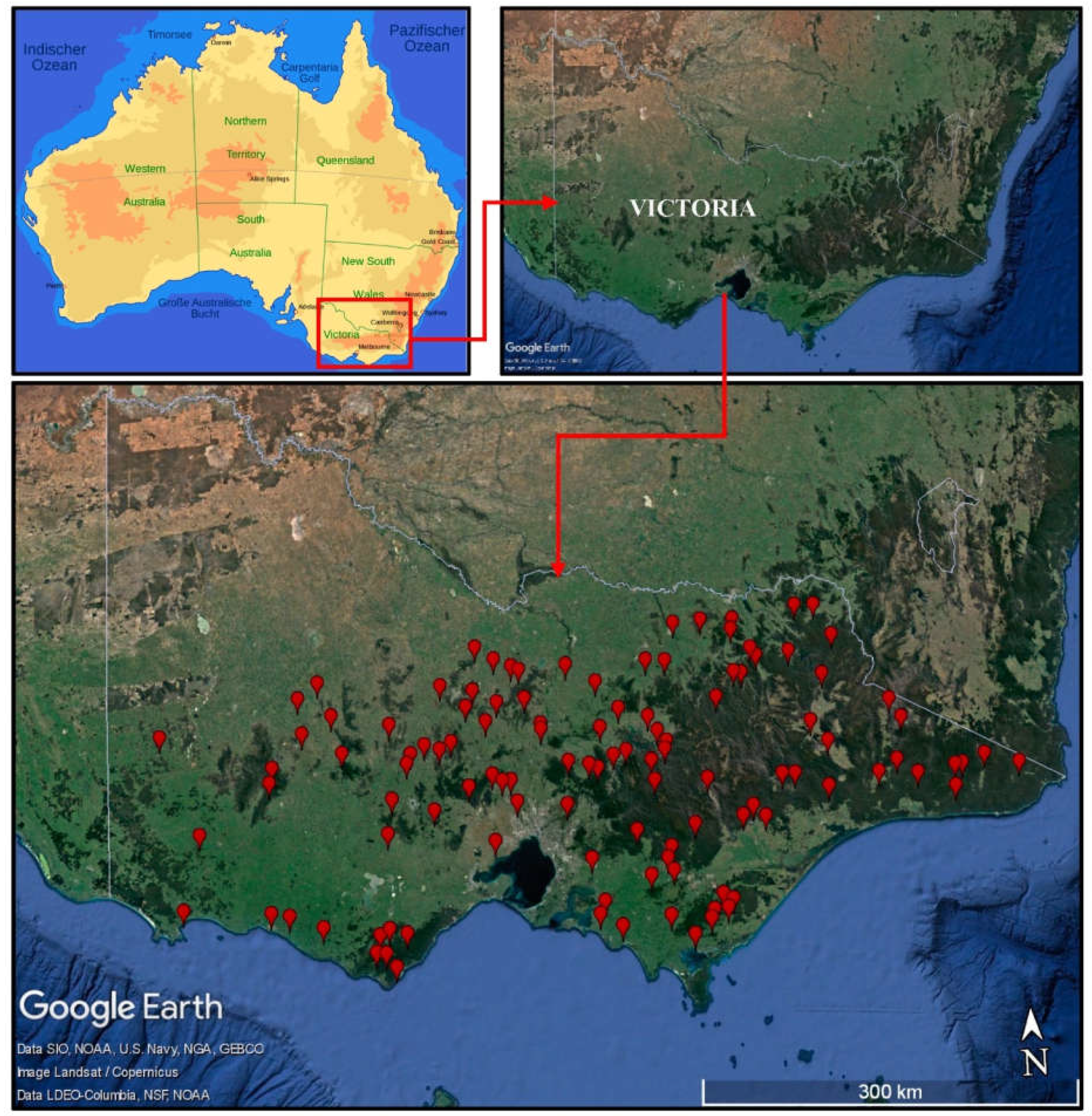
To summarise, GAM allows for the accounting of potential nonlinearities in RFFA, which cannot be achieved using linear models or simple variable transformations such as log or power methods. There has been little application of GAM in RFFA. To fill this knowledge gap, the aim of this study is to test the applicability of GAM to Victoria State of Australia and compare results with linear RFFA technique. This will assist to select more accurate RFFA technique for practical application in Victoria. The remainder of the paper is organised as follows: Section 2 presents the study area and dataset used; Section 3 explains the methodology used in this study; and the results and discussion of the study are presented in Section 4. Finally, discussion, and conclusions are provided in Section 5 and Section 6, respectively.

2. Study Area and Data

This study selects 114 gauged catchments from the State of Victoria, Australia. These are natural catchments with no major land use change and regulation. The size of the selected catchments ranges 3–997 km2 (mean: 317.5 km2 and median: 270.5 km2). Figure 1 shows the distributions of the selected catchments. The annual maximum flood record length ranges 26–62 years (mean 38 years); with 77% of the stations having record lengths of 34–42 years.
A total of eight catchment characteristics are selected, which are: catchment area (area); catchment shape factor (SF); design rainfall intensity with 2-year average recurrence interval (ARI) and 6-h duration (I6,2); mean annual rainfall (rain); mean annual evapotranspiration (evap); stream density (sden); mainstream slope (S1085); and fraction forest cover (forest). The catchment characteristics data used in this study are summarised in Table 1.

3. Methodology

3.1. Quantile Regression Technique (QRT)

The most commonly used relation between the flow statistics (e.g., flood quantile QT of return period T years) and the catchment characteristics (A1, A2,…, An) is the power-form function in the form [29]:
Q T = α 0 A 1 α 1 A 2 α 2 . A n α n ε 0
in which α 0 , α 1 ,…, α n are the coefficients of prediction equation, ε 0 is the multiplicative error term and n is the number of catchment characteristics. Alternatively, if the error term ( ε 0 ) is assumed to be additive then the power-form function becomes [30,31]:
Q   T = α 0 A 1 α 1 A 2 α 2 . A n α n + ε 0
For both cases, the regression coefficients/model parameters are not known and must be estimated using observed flow statistics and regional catchment characteristics. If the error term is multiplicative (Equation (3)), then the power-form model can be linearised by a logarithmic transformation and the parameters of the linearised model can be estimated by a linear regression technique. Taking log on both sides, Equation (3) can be expressed as:
log Q   T = log α 0 + α 1 log A 1 + α n log A n 1 + log ( ε 0 )
or in matrix form:
Y = X β + e
in which Y is the vector of flood statistics (quantile) from m sites (Y = log(QT)), β is the vector of regression coefficients (β =   α 0 ,   α 1 , …, α n ), X is the matrix of the physiographic characteristics or the explanatory variables (X =   log A 1 ) and e is the matrix of the error (e =   log ε 0 ). However, if the model error is additive (i.e., Equation (4)), it is not possible to linearise the power-form model by a logarithmic transformation and the model coefficients needs to be estimated by some nonlinear optimisation method.

3.2. GAM

Hastie and Tibshirani [6] were the first to propose generalised additive models (GAMs) in 1987. The mean of the response (dependent) variable is assumed to be dependent on an additive predictor via a link function in these models. GAM employs nonlinear functions of each predictor variable while retaining additivity. GAM, like generalised linear models (GLMs), allows the response probability distribution to be from any member of the exponential family. GAMs and GLMs differ only in that GAMs allow for unknown smooth functions in the linear predictor. GAM is a mathematical modelling technique in which the impact of predictive variables is captured using smooth functions that depend on the underlying patterns in the data, which may be nonlinear. GAM can be written as:
g E Y = α + s 1 x 1 + + s P x P
where Y is the dependent variable (here QT), E(Y) denotes the expected value, and g(E(Y)) denotes the link function that links the expected value to the predictor variables x1,…, xp. The terms s 1 x 1 ,…, s P x P denote smooth, nonparametric functions.
In general, a GAM has the below form:
g μ i = X i   * β + j = 1 m f j ( x i j )
where μ i   E Y i and Y i ∼an exponential family distribution.
Y i is a response variable, X i   * is the ith row of the model matrix for the strictly parametric model components; and f j are smooth functions of the covariates x j .

3.3. Cluster Analysis

Cluster analysis refers to a very broad set of techniques for finding subgroups or clusters in a data set. The objective of clustering the observations of a data set is to seek partitioning of observations into distinct groups so that the observations within each group are quite similar to each other (in relation to some attributes of the data), while observations in different groups are quite different from each other. In the adopted cluster analysis, the variables are standardised and are given equal weights. The hierarchical clustering is used with a combination of Wards-Manhattan method. K-Means clustering is also adopted in this study. All the eight predictor variables are used in the cluster analysis presented in this study.

3.4. Validation

In this study, K-fold cross validation is chosen to evaluate the RFFA model performance [26]. K-fold cross validation allows a randomly separate set of observations into k groups or folds which are approximately of equal size and fits the model using the rest of the samples except the first subset or fold. The held-out dataset is used to validate the statistical model through generating predictions using the statistical model based on the test dataset.
This procedure is repeated for k times. The mean and standard error values of k number of trials are summarised and used subsequently to evaluate the performance of the relationship between the tuning parameter(s) and model utility. The k-fold CV estimate is computed by averaging these values:
CV k = 1 k i = 1 k MSE i
The choice of k is usually 5 or 10, which depends on dataset. The difference in size between the training set and the resampling subsets gets smaller as the k increases. The bias of the technique becomes smaller (i.e., the bias is smaller for k = 10 than k = 5) with difference decrease. In this context, the bias is the difference between the estimated and true values of performance.
The following statistical measures were used to check the suitability and performance of the prediction model, which are:
Relative   Error   ( RE ) = Median   a b s Q p r e d Q o b s Q o b s
Ratio = Q p r e d Q o b s
where Q o b s = observed flood quantile at each site (estimated by a log-Pearson type 3 distribution); Q p r e d = predicted flood quantile at each site from regional prediction equation.

4. Results

The study is based on a variety of alternative groups, such as a combined group made up of all the 114 catchments and sub-groups formed by cluster analysis. Using hierarchical and k-means clustering techniques, four regions are formed: A1 (79 stations) and A2 (35 stations) from Wards-Manhattan clustering, and B1 (67 stations) and B2 (47 stations) from K-Means clustering. All these four groups and the combined sites in a single group are employed in the development of log-log linear models and GAM-based models.
Linear regression analysis is carried out using the dataset and backward stepwise procedure is followed to choose the catchment characteristics for model development. Table 2 shows the overall model statistics for the 6 different ARIs. The major statistical measures used are coefficient of determination (R2), p-value and standard error of estimate (SEE). R2 values range from 0.69 to 0.53, respectively for Q2 to Q100. The R2 values are found to be particularly small for higher ARIs, indicating that the variance explained by catchment characteristics becomes smaller, resulting in higher model error variance of prediction for higher ARI flood estimation. All the R2 values are modest to reasonable, indicating that the prediction equations are generally well-fitting. The SEE ranges from 0.22 to 0.32 for Q2 to Q100. SEE is found to be lowest in Q2 and highest in Q100. The predictor variables selected in the final model with the p-statistics value of ≤0.05 are shown in Table 2. From Table 2, the area and I6,2 appear to be the most important variables for estimating Q for log-log linear model. These two variables are common with all the prediction equations. The next most important predictor variable is found as rain which appears in every prediction equation except for Q2 and Q5. Only for Q2, sden is selected whereas rain is absent as predictor variable. For Q5, both rain and sden are selected as predictor variable. Overall, the prediction equations show consistency in selection of independent variables except for Q2 and Q5. Table 2 shows the variables of the developed prediction equations.
The log-log linear models are assessed using the Qpred/Qobs ratio and the median relative error (RE). 
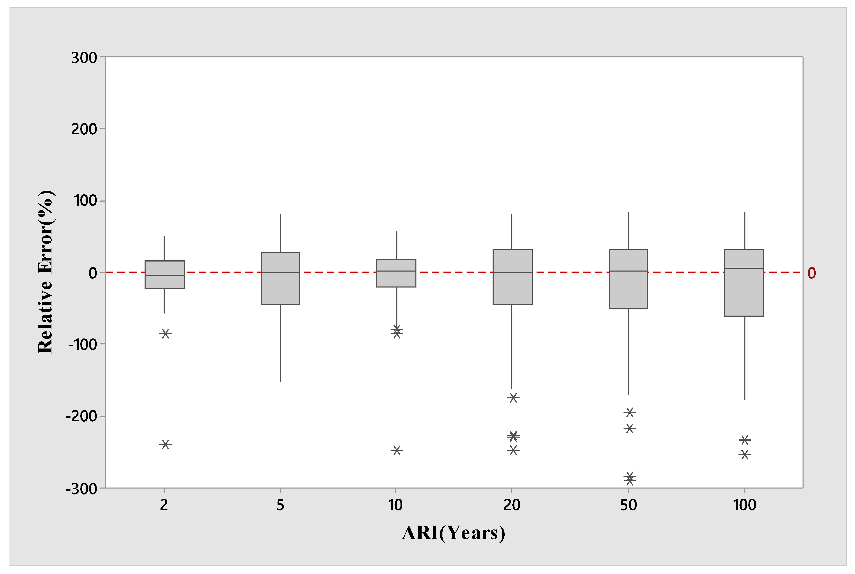
Figure 2 depicts boxplots of RE values for the log-log linear model for the combined group’s selected test catchments. Figure 2 shows that the median RE values (represented by the black line within a box) match very well with the 0:0 line for ARIs of 5 and 20 years and are relatively good for ARIs of 10 and 50 years. Some underestimation is observed for ARI of 2 years. The underestimation is remarkable for an ARI of 100 years. The ARI of 2 years has the lowest spread in the RE band, which is represented by the total spread of the box. The RE band for ten years ARI is very similar to the RE band for two years ARI. The RE band for 100 years ARI is more than twice than the RE bands for 2 and 10 years. These results show that in terms of RE, 10 years ARI achieve the best results, followed by 2 years ARI. Higher ARI flood quantiles are associated with a higher degree of spread in the RE, which could indicate a higher standard deviation of the estimate. This matches the findings of Haddad and Rahman [31] and Rahman et al. [32]. This is generally the case in RFFA as essentially, we are making predictions beyond the limits of the original data space.
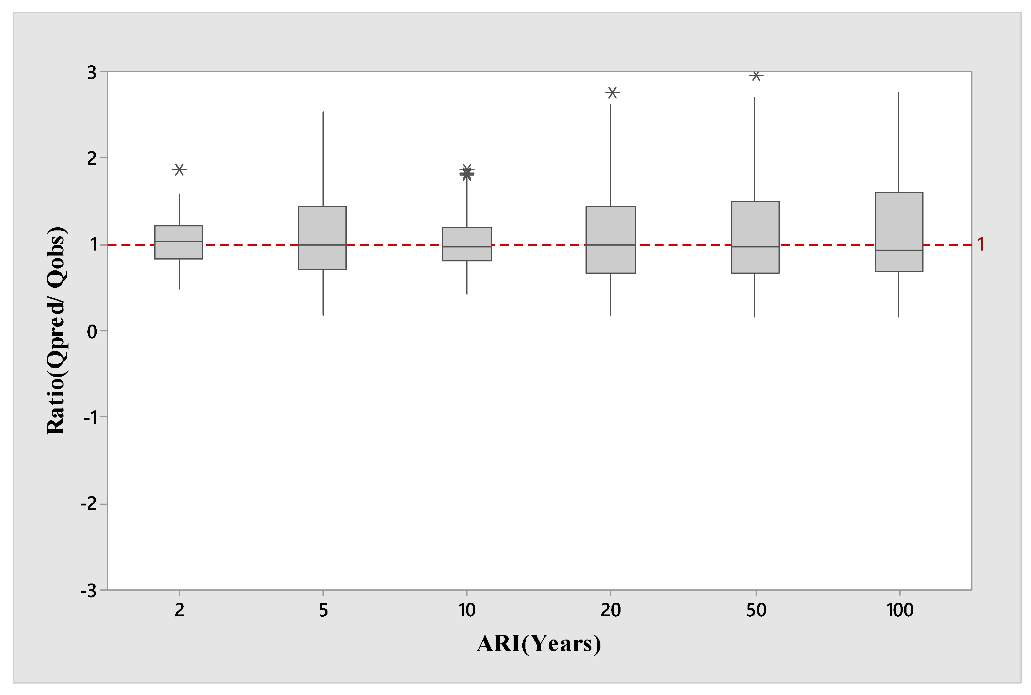
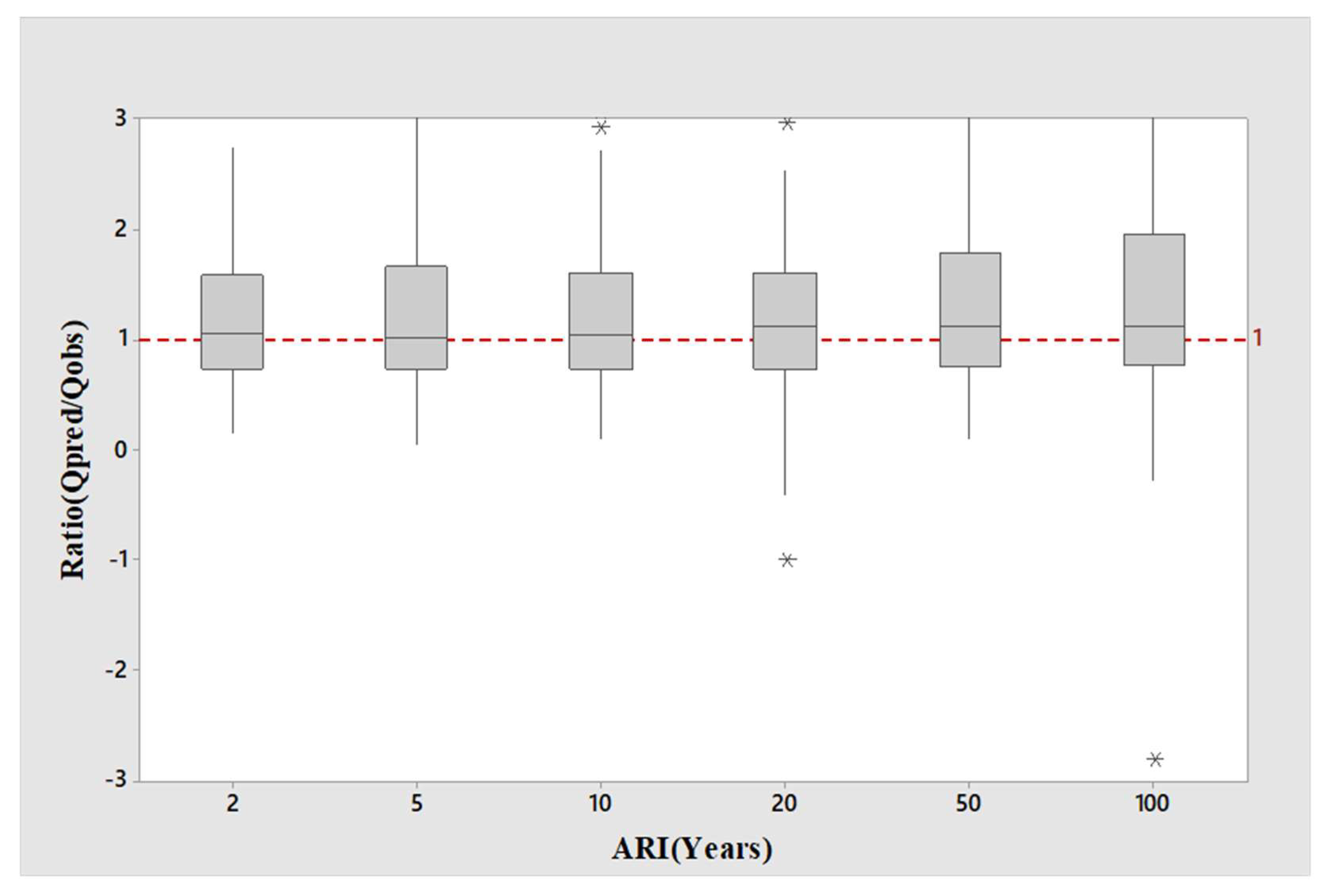
Figure 3 presents the boxplot of the Qpred/Qobs ratio values of the selected 114 catchments for the log-log linear model. It is found that the median Qpred/Qobs ratio values (represented by the thick black line within a box) are located closer to 1:1 line (the horizontal line in Figure 3), for ARIs of 2, 5,10, 20 and 50 years (the best agreement is for ARI of 20 years). However, for ARI of 100 years, the median Qpred/Qobs ratio value is located a short distance below the 1:1 line, and for ARI of 2 years, the median Qpred/Qobs ratio value is located a short distance above the 1:1 line. In terms of the spread of the Qpred/Qobs ratio values, ARI of 2 years exhibits the lowest spread followed by ARI of 10 years. Furthermore, the spreads of the Qpred/Qobs ratio values for 50 and 100 years are very similar, which are remarkably larger than 2 and 10 years.
For developing GAM model, predictor variables are selected using backward stepwise procedure. Table 3 shows overall GAM model (combined group) statistics for the 6 different ARIs. The major determinants are coefficient of determination (R2), generalised cross-validation (GCV) statistic and p-statistics. The R2 values range from 0.69 to 0.44; particularly, smaller R2 values are found for the higher ARIs indicating a weaker model. The R2 values for lower ARIs seem to be quite reasonable (0.62–0.69). The GCV values vary from 501 to 82, 994 for Q2 to Q100. The lowest value of GCV is found for Q2 and the highest one is found for Q100. This indicates that the cross-validation error increases with increasing ARIs.
The predictor variables for the individual models are selected based on the p-statistics of the predictor variables. The criterion of including a predictor variable in the final model is p ≤ 0.05. Table 3 contains all the selected predictor values for the models. The predictor variables area, I6,2 and evap appear to be the most important variables for estimating flood quantiles using GAM, as these three variables are common in all the prediction equations. The next most important predictor variable is rain, which appears in all the prediction models except for Q2. Another predictor variable, which is found statistically significant in Q2, Q5 and Q10 is sden. Overall, Q20, Q50 and Q100 models show a consistency in the selection of predictor variables (with area, I6,2 and evap). The selected predictor variables are shown in Table 3.
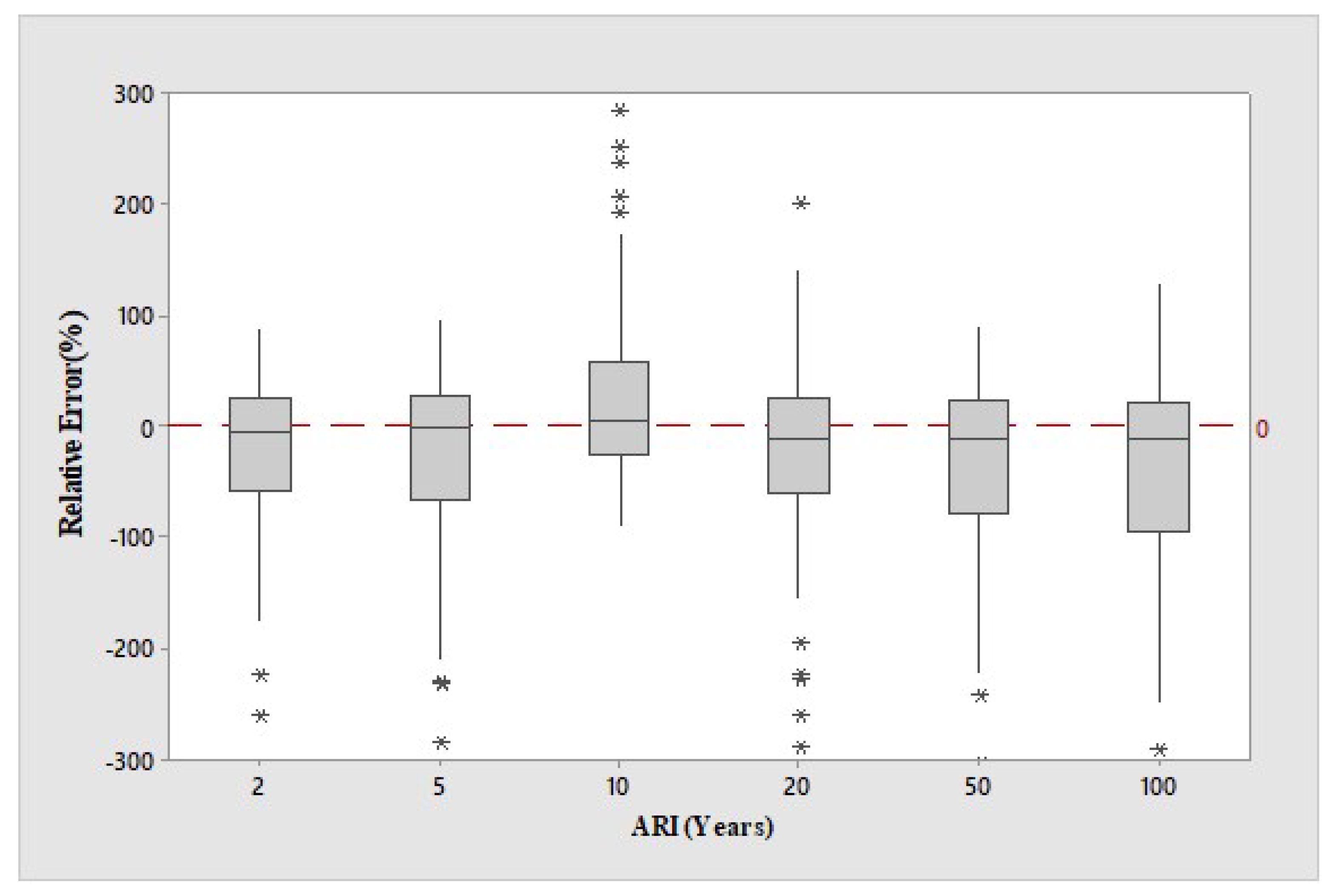
The boxplots of RE values for the GAM model of the combined group for the 6 ARIs are shown in Figure 4. For ARIs of 5 years, the median RE values match the 0:0 line very well, and reasonably well for ARIs of 2 and 10 years, respectively. Except for 10 years ARI, the GAM models underestimate by a small to moderate amount. In terms of the RE band, the ARIs of 2 and 10 years have nearly identical spreads, which are also smaller than the remaining ARIs. The RE bands for 50 and 100 years of ARIs are very similar, which indicates a similar level of prediction error for these ARIs by the GAM. These results show that in terms of RE, the best overall result (for the combined group) for the GAM model is achieved for 2 years ARI. Overall, the performances of the GAM models (as indicated by the RE bands) for the combined group do not show a large variation across the six ARIs.
Figure 5 presents the boxplots of the Qpred/Qobs ratio values associated with the GAM models for the combined group for the six ARIs. It is found that the median Qpred/Qobs ratio values are located very close to 1:1 line, for ARIs of 5 and 10 years, showing the best agreement for ARI of 10 years. However, for all the ARIs, the median Qpred/Qobs ratio values are located within a short distance above the 1:1 line except for ARI of 100 years. For this ARI, there is a noticeable overestimation by the GAM model. These results indicate a slight to noticeable overestimation of the predicted flood quantiles for all the ARIs. In terms of the spread of the Qpred/Qobs ratio values, ARI of 2 years exhibits the lowest spread, whereas 10 and 20 years of ARIs show similar spread. Furthermore, the spreads of the Qpred/Qobs ratio values for 50 and 100 years of ARIs are very similar, which are remarkably larger than 2, 5 and 10 years of ARIs.
Table 4 compares the R2 values of the ten different RFFA models. From Table 4, R2 values from GAM models are found to be higher than those from the respective log-log linear models for smaller ARIs. It has also been revealed that GAM models based on clustering groups produce better results, for example, models for smaller ARIs produce higher R2 values. For example, the R2 values of Q2, Q5, and Q10 for GAM models in the combined group are 0.83, 0.73, and 0.70, respectively, which are 10%, 8%, and 4% higher than the respective log-log linear models. GAM models, on the other hand, have lower R2 values than respective log-log linear models for higher ARIs (e.g., 0.67, 0.58 and 0.51, which are 1%, 10% and 17% lower than respective log-log linear model). Furthermore, the GAM models of clustering groups produce better results for Q2 with a maximum value of 0.90. Overall, the log-log linear models give better performance for higher ARIs (i.e., 20, 50 and 100 years) and GAM models show better performance for smaller ARIs (i.e., 2, 5 and 10 years).
In Table 5, the median RE values are summarised for the log-log linear and GAM models for the combined and four clustering groups. The median RE values are calculated considering the absolute relative error value (RE) of the test catchments. The highest RE is 59.94%, which is found for log-log linear model for the clustering group A2 for 100 years of ARI, and the lowest RE is 16.8%, which is found for the GAM model of group B1 data for 2 years ARI.
For the log-log linear models, median RE values range from 18.73% to 59.94%. The smallest and highest median RE values are found for the log-log linear models of the combined group for 2 years of ARI and clustering group A2 for 100 years ARI, respectively. From the overall median RE values for the log-log linear models, the smallest result is found from clustering group A1 with median RE of 31.11%. The overall highest median RE value for the log-log linear model is found from clustering group A2 with the value of 42.40%. The overall median RE values range from 31.11% to 42.40%, which indicate that the median RE does not differ much between different groups of the log-log linear models. Lowest values of RE are mostly found from 2 years of ARI for log-log linear model, which range from 18.73% to 30.33%, which are for the combined group and clustering group B1, respectively. The highest values of RE are found for 100 years ARI for the log-log linear models, which range from 37% to 59.94%, which are for clustering groups B1 and A2, respectively.
In the case of GAM, median RE values range from 16.8% to 53.38%. The smallest and highest median RE values are found for 2 years of ARI for clustering group B1, and for 100 years of ARI for clustering group A1, respectively. With respect to the overall median RE, the smallest value is found for the clustering group B1 with median RE of 35.10%. The overall highest median RE value is found for clustering group A2 (43.73%). The overall median RE values range from 35.10% to 43.73% for the GAM models. Lower values of median RE are mostly found for 2 years of ARI for the GAM, which range from 16.80% to 39.31% (for the clustering groups B1 and A2). The highest values of RE are found for 100 years of ARI for the GAM, which range from 39.04% (clustering group B2) to 53.38% (clustering group A1). It is observed that in most cases, the median RE values of GAM are greater than respective log-log linear models. For group A2, median RE values of the GAM models are lower than the log-log linear models for ARIs of 10, 20, 50 and 100 years. However, considering overall performance of median RE, log-log linear model is found to have better accuracy than GAM.
In Table 6 median ratio (Qpred/Qobs) values are summarised for 5 log-log linear models and 5 GAM models. The median ratio values are important as these are an effective indicator of overestimation or underestimation (i.e., a measure of bias) of the prediction model. The highest Qpred/Qobs ratio is 1.16, which is found for the log-log linear model for clustering group A1 for ARI of 50 years, and the lowest median Qpred/Qobs ratio is 0.83, which is found for GAM model for clustering group A2 data of 10 years of ARI.
For log-log linear models, median Qpred/Qobs ratio values range from 0.90 to 1.09. The smallest and highest median ratio values are found for 100 years of ARI for the log-log linear model of the clustering group B2 and log-log linear model of the clustering group B1, respectively. The overall smallest median Qpred/Qobs ratio values for the log-log linear models are found as 0.96, which is for the clustering group B2 and the highest median Qpred/Qobs ratio value for log-log linear model is found for the clustering group B1, which is 1.01. The overall median ratio values range from 0.96 to 1.01, which indicate a very small percentage of difference between different groups of the log-log linear models. Most of the median Qpred/Qobs ratio values obtained from the log-log linear model are in the range of 0.95 to 0.99, which indicate a slight underestimation in the prediction of flood quantiles. The best result is obtained for 20 and 5 years ARIs for the combined group, with the median ratio value of 1.00. In summary, log-log linear model-based RFFA techniques show a very reasonable and consistent median Qpred/Qobs ratio value.
In the case of GAM, median Qpred/Qobs ratio values range from 0.83 to 1.16. The smallest and highest median Qpred/Qobs ratio values are found for ARIs of 10 years for the clustering group A2 and 50 years ARI for the clustering group A1, respectively. The overall smallest median Qpred/Qobs ratio value for GAM is found for clustering group A2 with median Qpred/Qobs ratio of 0.97. The overall highest median Qpred/Qobs ratio value is found for combined group with median ratio of 1.08. The overall median Qpred/Qobs ratio value ranges from 0.98 to 1.08, which indicates that GAM tends to make an overestimation. Moreover, the overall median Qpred/Qobs ratio values for the GAM models are higher compared with respective log-log linear models. Most of the median Qpred/Qobs ratio values are found above 1.00 for the GAM models, which indicates again an overestimation. Lower values of median Qpred/Qobs ratio values for GAM are mostly found for the clustering group A2 that range from 0.83 to 1.14, which are comparatively lower than median Qpred/Qobs ratio values of the log-log linear models of the clustering group A2. For clustering group A2, median Qpred/Qobs ratio values are lower for the GAM than the log-log linear models for higher ARIs i.e., for 10, 20 and 50 years. However, in most cases, the median Qpred/Qobs ratio values of GAM are greater than the respective log-log linear models. Overall, median Qpred/Qobs ratio values indicate that the log-log linear models produce better predictions than GAM in the higher ARIs.

5. Discussion

This study compares GAM and QRT for Victoria, Australia by using data from 114 gauged catchments. Based on independent validation, it is found that GAM provides more accurate quantile estimates than QRT for smaller return periods, and QRT outperforms GAM for higher return periods. Overall, the median relative error values for 2, 5 and 10 years ARIs in this study are found to be 16–41%, which are smaller than similar other studies [33,34]. For example, Zalnezhad et al. [35] applied artificial intelligence based RFFA techniques for south-east Australia and reported a median relative error value of 37–43% for 2 to 10 years ARIs. For south-east Australia Aziz et al. [3] applied non-linear RFFA techniques and reported a median relative error value of 37–72% for ARIs of 2 to 10 years. Ali and Rahman [36] applied ordinary kriging to Victoria and reported a median relative error value of 28–36% for 2 to 10 years ARIs. Hence, GAM has performed better than these studies [3,35,36] for 2 to 10 years ARI range.
To enhance the accuracy of the developed RFFA models, a greater number of stations with longer streamflow data should be adopted in near future when such data is available. Furthermore, additional predictor variables should be tested to enhance model accuracy. For model validation, leave-one-out and Monte Carlo cross validation should also be applied.

6. Conclusions

GAM handles nonlinearity in RFFA better than the commonly used log-log linear models, especially for smaller return periods (e.g., 2 to 10 years). It is found that none of the RFFA models examined in this study perform equally well across all the six ARIs in terms of all the adopted statistical measures. Based on overall average values of R2, median RE and median Qpred/Qobs ratio values, it is found that log-log linear models from clustering group A1 outperform the respective GAM models. However, for smaller ARIs (i.e., 2, 5, and 10 years), GAM based RFFA models perform almost similar or better than the log-log linear models. This is as expected, since for smaller floods (i.e., for smaller ARIs), catchments generally tend to behave more non-linearly, i.e., a higher loss value. For higher ARIs (e.g., 50 and 100 years), catchments behave more linearly, hence log-log linear regression models are expected to perform better, which is confirmed in this study. There are predictor variables, which were previously found by [33,34] to be insignificant in RFFA, but are found statistically significant for the GAM models developed here. For example, evap is found statistically significant for most of the GAM models as opposed to previous RFFA studies in Australia. It is found that area, I6,2 and rain are the most significant predictor variables for the log-log linear models. For the GAM models, the most important predictor variables are area, I6,2, rain and evap.
Except in one case, cluster analysis has not produced superior groups in RFFA. The median RE values for the log-log linear models based on clustering group A1 (consisting of 79 catchments) are found to be the lowest (29% to 37%) among all the five groups; however, the other clustering groups perform poorly. The findings of this study are expected to provide guidance in updating the RFFA techniques in the Australian Rainfall Runoff guideline. The future research should be focused on using more predictor variables in RFFA studies based on GAM. Also, GAM should be applied to other Australian states using a large number of gauging stations.

Author Contributions

F.N. conducted the data analysis and drafted the manuscript, O.U.L. edited the manuscript, enhanced writing and formatted the article, K.H. wrote part of the manuscript and improved the literature review, M.A.A. edited the manuscript and enhanced the discussion, and A.R. supervised the analysis and enhanced writing. All authors have read and agreed to the published version of the manuscript.

Funding

This research received no external funding.

Institutional Review Board Statement

Not applicable.

Informed Consent Statement

Not applicable.

Data Availability Statement

Streamflow data used in this study can be obtained from Victorian Government by paying a prescribed fee.

Conflicts of Interest

The authors declare no conflict of interest.

References

  1. Micevski, T.; Hackelbusch, A.; Haddad, K.; Kuczera, G.; Rahman, A. Regionalisation of the Parameters of the Log-Pearson 3 Distribution: A Case Study for New South Wales, Australia. Hydrol. Process. 2015, 29, 250–260. [Google Scholar] [CrossRef]
  2. Chebana, F.; Charron, C.; Ouarda, T.B.M.J.; Martel, B. Regional Frequency Analysis at Ungauged Sites with the Generalized Additive Model. J. Hydrometeorol. 2014, 15, 2418–2428. [Google Scholar] [CrossRef] [Green Version]
  3. Aziz, K.; Rai, S.; Rahman, A. Design Flood Estimation in Ungauged Catchments Using Genetic Algorithm-Based Artificial Neural Network (GAANN) Technique for Australia. Nat. Hazards 2015, 77, 805–821. [Google Scholar] [CrossRef]
  4. Alobaidi, M.H.; Marpu, P.R.; Ouarda, T.B.M.J.; Chebana, F. Regional Frequency Analysis at Ungauged Sites Using a Two-Stage Resampling Generalized Ensemble Framework. Adv. Water Resour. 2015, 84, 103–111. [Google Scholar] [CrossRef]
  5. Haddad, K.; Rahman, A. Regional Flood Frequency Analysis: Evaluation of Regions in Cluster Space Using Support Vector Regression. Nat. Hazards 2020, 102, 489–517. [Google Scholar] [CrossRef]
  6. Hastie, T.; Tibshirani, R. Generalized Additive Models: Some Applications. J. Am. Stat. Assoc. 1987, 82, 371. [Google Scholar] [CrossRef]
  7. Wood, S.N. Generalized Additive Models; Chapman and Hall/CRC: Boca Raton, FL, USA, 2017. [Google Scholar] [CrossRef] [Green Version]
  8. Morlini, I. On Multicollinearity and Concurvity in Some Nonlinear Multivariate Models. Stat. Methods Appl. 2006, 15, 3–26. [Google Scholar] [CrossRef]
  9. Schindeler, S.K.; Muscatello, D.J.; Ferson, M.J.; Rogers, K.D.; Grant, P.; Churches, T. Evaluation of Alternative Respiratory Syndromes for Specific Syndromic Surveillance of Influenza and Respiratory Syncytial Virus: A Time Series Analysis. BMC Infect. Dis. 2009, 9, 190. [Google Scholar] [CrossRef] [PubMed] [Green Version]
  10. Wen, L.; Rogers, K.; Ling, J.; Saintilan, N. The Impacts of River Regulation and Water Diversion on the Hydrological Drought Characteristics in the Lower Murrumbidgee River, Australia. J. Hydrol. 2011, 405, 382–391. [Google Scholar] [CrossRef]
  11. Wood, S.N.; Augustin, N.H. GAMs with Integrated Model Selection Using Penalized Regression Splines and Applications to Environmental Modelling. Ecol. Modell. 2002, 157, 157–177. [Google Scholar] [CrossRef] [Green Version]
  12. Ouarda, T.B.M.J.; Charron, C.; Marpu, P.R.; Chebana, F. The Generalized Additive Model for the Assessment of the Direct, Diffuse, and Global Solar Irradiances Using SEVIRI Images, With Application to the UAE. IEEE J. Sel. Top. Appl. Earth Obs. Remote Sens. 2016, 9, 1553–1566. [Google Scholar] [CrossRef] [Green Version]
  13. Bayentin, L.; El Adlouni, S.; Ouarda, T.B.M.J.; Gosselin, P.; Doyon, B.; Chebana, F. Spatial Variability of Climate Effects on Ischemic Heart Disease Hospitalization Rates for the Period 1989-2006 in Quebec, Canada. Int. J. Health Geogr. 2010, 9, 5. [Google Scholar] [CrossRef] [PubMed] [Green Version]
  14. Clifford, S.; Low Choy, S.; Hussein, T.; Mengersen, K.; Morawska, L. Using the Generalised Additive Model to Model the Particle Number Count of Ultrafine Particles. Atmos. Environ. 2011, 45, 5934–5945. [Google Scholar] [CrossRef]
  15. Guan, B.; Hsu, H.; Wey, T.; Tsao, L. Modeling Monthly Mean Temperatures for the Mountain Regions of Taiwan by Generalized Additive Models. Agric. For. Meteorol. 2009, 149, 281–290. [Google Scholar] [CrossRef]
  16. Haddad, K.; Vizakos, N. Air Quality Pollutants and Their Relationship with Meteorological Variables in Four Suburbs of Greater Sydney, Australia. Air Qual. Atmos. Health 2021, 14, 55–67. [Google Scholar] [CrossRef]
  17. Tisseuil, C.; Vrac, M.; Lek, S.; Wade, A.J. Statistical Downscaling of River Flows. J. Hydrol. 2010, 385, 279–291. [Google Scholar] [CrossRef]
  18. Morton, R.; Henderson, B.L. Estimation of Nonlinear Trends in Water Quality: An Improved Approach Using Generalized Additive Models. Water Resour. Res. 2008, 44. [Google Scholar] [CrossRef]
  19. Asquith, W.H.; Herrmann, G.R.; Cleveland, T.G. Generalized Additive Regression Models of Discharge and Mean Velocity Associated with Direct-Runoff Conditions in Texas: Utility of the U.S. Geological Survey Discharge Measurement Database. J. Hydrol. Eng. 2013, 18, 1331–1348. [Google Scholar] [CrossRef]
  20. Wang, Y.; Li, J.; Feng, P.; Hu, R. A Time-Dependent Drought Index for Non-Stationary Precipitation Series. Water Resour. Manag. 2015, 29, 5631–5647. [Google Scholar] [CrossRef]
  21. Garcia Galiano, S.G.; Olmos Gimenez, P.; Giraldo-Osorio, J.D. Assessing Nonstationary Spatial Patterns of Extreme Droughts from Long-Term High-Resolution Observational Dataset on a Semiarid Basin (Spain). Water 2015, 7, 5458–5473. [Google Scholar] [CrossRef] [Green Version]
  22. Shortridge, J.E.; Guikema, S.D.; Zaitchik, B.F. Empirical Streamflow Simulation for Water Resource Management in Data-Scarce Seasonal Watersheds. Hydrol. Earth Syst. Sci. Discuss. 2015, 12, 11083–11127. [Google Scholar] [CrossRef]
  23. Li, L.; Wu, K.; Jiang, E.; Yin, H.; Wang, Y.; Tian, S.; Dang, S. Evaluating Runoff-Sediment Relationship Variations Using Generalized Additive Models That Incorporate Reservoir Indices for Check Dams. Water Resour. Manag. 2021, 35, 3845–3860. [Google Scholar] [CrossRef]
  24. Rahman, A.; Charron, C.; Ouarda, T.B.M.J.; Chebana, F. Development of Regional Flood Frequency Analysis Techniques Using Generalized Additive Models for Australia. Stoch. Environ. Res. Risk Assess. 2018, 32, 123–139. [Google Scholar] [CrossRef]
  25. Rahman, A.S.; Khan, Z.; Rahman, A. Application of Independent Component Analysis in Regional Flood Frequency Analysis: Comparison between Quantile Regression and Parameter Regression Techniques. J. Hydrol. 2020, 581, 124372. [Google Scholar] [CrossRef]
  26. Haddad, K.; Rahman, A.; A Zaman, M.; Shrestha, S. Applicability of Monte Carlo Cross Validation Technique for Model Development and Validation Using Generalised Least Squares Regression. J. Hydrol. 2013, 482, 119–128. [Google Scholar] [CrossRef]
  27. Mohit Isfahani, P.; Modarres, R. The Generalized Additive Models for Non-Stationary Flood Frequency Analysis. Iran-Water Resour. Res. 2020, 16, 376–387. [Google Scholar]
  28. Msilini, A.; Charron, C.; Ouarda, T.B.M.J.; Masselot, P. Flood Frequency Analysis at Ungauged Catchments with the GAM and MARS Approaches in the Montreal Region, Canada. Can. Water Resour. J./Rev. Can. Ressour. Hydr. 2022, 47, 111–121. [Google Scholar] [CrossRef]
  29. Thomas, D.M.; Benson, M.A. Generalization of Streamflow Characteristics from Drainage-Basin Characteristics; Geological Survey Water-Supply Paper 1975; United States Government Printing Office: Washington, WA, USA, 1975.
  30. McCuen, R.H.; Leahy, R.B.; Johnson, P.A. Problems with Logarithmic Transformations in Regression. J. Hydraul. Eng. 1990, 116, 414–428. [Google Scholar] [CrossRef]
  31. Haddad, K.; Rahman, A. Regional Flood Frequency Analysis in Eastern Australia: Bayesian GLS Regression-Based Methods within Fixed Region and ROI Framework—Quantile Regression vs. Parameter Regression Technique. J. Hydrol. 2012, 430, 142–161. [Google Scholar] [CrossRef]
  32. Rahman, A.; Haddad, K.; Zaman, M.; Kuczera, G.; Weinmann, P.E. Design Flood Estimation in Ungauged Catchments: A Comparison between the Probabilistic Rational Method and Quantile Regression Technique for NSW. Aust. J. Water Resour. 2011, 14, 127–140. [Google Scholar] [CrossRef]
  33. Rahman, A.; Haddad, K.; Kuczera, G.; Weinmann, E. Regional Flood Methods. In Australian Rainfall & Runoff, Chapter 3, Book 3; Ball, J., Babister, M., Nathan, R., Weeks, B., Weinmann, E., Retallick, M., Testoni, I., Eds.; Commonwealth of Australia: Canberra, Australia, 2016. [Google Scholar]
  34. Rahman, A.; Haddad, K.; Haque, M.; Kuczera, G.; Weinmann, P.E. Australian Rainfall and Runoff Project 5: Regional Flood Methods: Stage 3 Report (No. P5/S3, p. 025); Technical Report; Geoscience Australia and the National Committee for Water Engineering: Symonston, Australia, 2015.
  35. Zalnezhad, A.; Rahman, A.; Nasiri, N.; Vafakhah, M.; Samali, B.; Ahamed, F. Comparing Performance of ANN and SVM Methods for Regional Flood Frequency Analysis in South-East Australia. Water 2022, 14, 3323. [Google Scholar] [CrossRef]
  36. Ali, S.; Rahman, A. Development of a Kriging Based Regional Flood Frequency Analysis Technique for South-East Australia, Natural Hazards. 2022. Available online: https://link.springer.com/article/10.1007/s11069-022-05488-4 (accessed on 6 November 2022).
Figure 1. Location of study catchments in Victoria, Australia.
Water 14 03627 g001
Figure 2. Boxplots of relative error (RE) values for log-log linear model of combined group (* represents outliers).
Water 14 03627 g002
Figure 3. Boxplots of Qpred/Qobs ratio values for log-log linear model of combined group (* represents outliers).
Water 14 03627 g003
Figure 4. Boxplots of RE values for the GAM model of combined group (* represents outliers).
Water 14 03627 g004
Figure 5. Boxplots of Qpred/Qobs ratio values for GAM model of combined group (* represents outliers).
Water 14 03627 g005
Table 1. Summary of catchment characteristics data.
VariableUnitNotationMinMeanMaxSD
Catchment areakm2area3317.54997244.65
Catchment shape factor-SF0.2810.791.43410.22
Mainstream slopem/kmS10850.813.3869.912.30
Stream densitykm/km2sden0.521.534.250.53
Fraction of catchment covered by forest-forest0.010.5910.35
Rainfall intensity (6-h duration and 2-year ARI)mm/hI6,224.634.2946.75.27
Mean annual rainfallmmrain484.39931.641760.81319.01
Mean annual potential evapotranspirationmmevap925.91035.471155.342.80
Table 2. Model statistics for log-log linear model of combined group.
EquationPredictor VariablesRegression Coefficient (β)Standard ErrorStandard Error of Estimate (SEE)R2D.F
log Q2(constant)−2.420.520.220.69110
log (area)0.680.04
log (I6,2)1.480.33
log (sden)0.390.15
log Q5(constant)−1.600.570.230.67109
log (area)0.680.05
log (I6,2)1.740.41
log (rain)−0.290.19
log (sden)0.310.16
log Q10(constant)−1.250.620.250.63110
log (area)0.660.05
log (I6,2)2.140.43
log (rain)−0.530.20
log Q20(constant)−1.000.660.270.61110
log (area)0.660.05
log (I6,2)2.300.46
log (rain)−0.660.21
log Q50(constant)−0.790.730.300.57110
log (area)0.660.06
log (I6,2)2.450.51
log (rain)−0.760.23
log Q100(constant)−0.700.780.320.53110
log (area)0.660.06
log (I6,2)2.540.54
log (rain)−0.810.25
Table 3. Important model statistics for GAM models of combined group.
Flood QuantilePredictor VariablesDeviance Explained (%)Generalized Cross Validation Statistic (GCV)R2F Value
Q2area73.70501.610.6930.199
I6,25.37
evap7.59
sden6.07
Q5area71.33201.900.6626.69
I6,24.898
rain3.073
evap6.278
sden4.492
Q10area67.608437.800.6223.46
I6,24.67
rain6.91
evap5.02
sden3.15
Q20area62.2018974.000.5617.39
I6,24.41
rain8.95
evap3.99
Q50area56.2045823.000.509.96
I6,28.56
rain12.12
evap3.31
Q100area48.4082994.000.4417.32
I6,211.53
rain10.87
evap2.46
Table 4. R2 values of the GAM and log-log linear models for 10 cases.
Flood QuantileCombined GroupGroup (A1)Group (A2)Group (B1)Group (B2)
log-log Linear ModelGAMlog-log Linear ModelGAMlog-log Linear ModelGAMlog-log Linear ModelGAMlog-log Linear ModelGAM
Q20.690.690.740.830.690.750.780.900.650.712
Q50.670.660.720.790.550.6760.740.830.570.626
Q100.630.620.700.730.480.5540.710.780.480.506
Q200.610.560.680.670.430.5060.690.710.420.456
Q500.570.500.650.580.320.4370.650.600.390.322
Q1000.530.440.620.510.270.360.620.550.320.30
Overall0.620.580.690.690.460.550.700.730.470.49
Table 5. Median RE values (%) for the GAM and log-log linear model based RFFA techniques for ten cases.
Flood QuantileCombined GroupGroup (A1)Group (A2)Group (B1)Group (B2)
log-log Linear ModelGAMlog-log Linear ModelGAMlog-log Linear ModelGAMlog-log Linear ModelGAMlog-log Linear ModelGAM
Q218.7334.8129.5622.5223.1039.3130.3316.8025.8233.24
Q532.8833.8828.6033.1034.6941.4628.2028.9231.9741.11
Q1019.3633.7527.4731.9640.5440.2927.3734.4633.0538.17
Q2034.5134.0530.7439.5343.0242.3529.3742.4736.6945.82
Q5040.4142.6733.2540.1253.1049.5937.4242.0839.2931.38
Q10040.9949.0937.0553.3859.9449.3737.0045.9042.6339.04
Overall31.1538.0431.1136.7742.4043.7331.6135.1034.9138.13
Table 6. Median Qpred/Qobs ratio values for the GAM and log-log linear model based RFFA techniques for 10 cases.
Flood QuantileCombinedGroup (A1)Group (A2)Group (B1)Group (B2)
log-log Linear ModelGAMlog-log Linear ModelGAMlog-log Linear ModelGAMlog-log Linear ModelGAMlog-log Linear ModelGAM
Q21.031.071.041.011.001.131.011.051.041.10
Q51.001.020.951.030.991.040.981.001.030.95
Q100.971.040.941.060.980.830.961.020.921.04
Q201.001.120.971.101.010.841.011.060.940.98
Q500.981.121.021.160.950.861.051.140.940.98
Q1000.941.121.021.120.951.141.091.130.901.01
Overall0.991.080.991.080.980.971.011.070.961.01
Publisher’s Note: MDPI stays neutral with regard to jurisdictional claims in published maps and institutional affiliations.

