Multiscale Interactions of Climate Variability and Rainfall in the Sogamoso River Basin: Implications for the 1998–2000 and 2010–2012 Multiyear La Niña Events

Abstract

In this research, we explored rainfall variability in the Sogamoso River Basin (SRB), its relationship with multiple scales of variability associated with El Niño–Southern Oscillation (ENSO), and the implications for rainfall prolongation during multiyear La Niña events. First, we examined time-frequency rainfall variations in the SRB based on the standardized precipitation index (SPI) from 1982 to 2019, using wavelet transform and principal component analysis (PCA). In addition, we applied wavelet analysis to investigate the links at different time scales between ENSO and the main mode of rainfall variability in the SRB. Finally, we explored the role that each scale of variability played in the prolongation and intensity of rainfall in the SRB during the 1998–2000 and 2010–2012 multiyear La Niña events. The results of the wavelet analyses revealed significant ENSO relationships affecting SRB rainfall at three different scales: quasi-biennial (2–3-years) between 1994 and 2002, as well as from 2008 to 2015; interannual (5–7 years) from 1995 to 2011; and quasi-decadal (9–12 years) from 1994 to 2012. This indicates that multiyear events are a consequence of the interaction of several scales of variability rather than a unique scale. During the 1998–2000 event, El Niño conditions were observed during the first half of 1998; subsequently, a cooling of the central and eastern tropical Pacific (western tropical Pacific) on the quasi-biennial (interannual) scale was observed during 1999; in 2000, only La Niña conditions were observed on the interannual scale. Therefore, during this event, the quasi-biennial (interannual) scale promoted wet conditions in the Caribbean, the Andes, and the Colombian Pacific from June–August (JJA) 1998 to JJA 1999 (during 1999–2000). During the 2010–2012 La Niña event, the interbasin sea surface temperature gradient between the tropical Pacific and tropical North Atlantic contributed to strengthening (weakening) of the Choco jet (Caribbean low-level jet) on the quasi-biennial scale during 2010, and the interannual scale prolonged its intensification (weakening) during 2011–2012, acting to extend the rainy periods over most of the Colombian territory. Variations on quasi-decadal scales were modulated by the Pacific decadal oscillation (PDO), resulting in a further intensification of the 2010–2012 La Niña event, which developed under conditions of the cold PDO (CPDO) phase, whereas the 1998–2000 La Niña occurred during the transition from warm (WPDO, 1977–1998) to cold (CPDO, 2001–2015) conditions. These results indicate that the interaction of quasi-biennial to quasi-decadal scales of variability could play a differential role in the configuration and prolongation of rainfall events in the SRB.

1. Introduction

According to the sixth report of the Intergovernmental Panel on Climate Change, anthropogenic climate change leads to increased frequency and intensity of extreme precipitation events due to changes in temperature and water vapor, increasing the magnitude of precipitation extremes in the range of 4% to 8% per degree Celsius of surface warming [1]. Therefore, there is a need to understand the natural variations in precipitation in a given region, as the occurrence of droughts or excessive precipitation generates economic and social impacts [2,3].

It is widely recognized that a large set of extreme hydrological and meteorological events around the world are triggered by the El Niño–Southern Oscillation (ENSO) phenomenon, considered the most important modulator of global hydroclimatology at interannual time scales [4]. ENSO has two phases, which are the result of atmosphere–ocean interactions reflected by sea surface temperature (SST) conditions in the tropical Pacific basin [5,6], where the SST is higher (lower) than the climatological average during an El Niño (La Niña) event [4,7]. According to Aceituno et al. [8] and Cai et al. [6], in South America, the two phases, El Niño and La Niña, influence the hydroclimatology of the Andean region, recognizing ENSO as the most important source of interannual variability in northern South America; El Niño (La Niña) is linked with below (above)-average precipitation, soil moisture, and river discharges [9].

In Colombia—mainly in the central, northern, and western regions—El Niño (La Niña) events generate a decrease (increase) in precipitation, streamflow, and soil moisture [10,11,12], which can lead to forest fires, droughts and flash floods, prolonged flooding, and landslides in the plains, with adverse socioeconomic consequences for the country [6,13,14]. In the last forty years, the El Niño (La Niña) events recorded during 1997–1998 and 2015–2016 (1998–2000 and 2010–2012) stand out as the strongest events, with significant negative consequences for the country [6,9,11,15,16,17], mainly during La Niña events, which were of longer duration than El Niño events. According to Iwakiri et al. [18], this behavior is due to the strong transition asymmetry of ENSO, whereby El Niño concludes quickly, whereas some La Niña events often last more than two years and are defined as multiyear events [7,18,19]. The persistence of multiyear El Niño and La Niña events exacerbate the induced climate impacts, generating persistent floods and droughts worldwide [9,20,21,22,23].

The 2010–2012 multiyear La Niña caused prolonged flash floods due to above-normal rainfall in most of Colombia [14,17], resulting in losses and damage to infrastructure, crops, and livelihoods [14]. A total of 1233 floods, 778 landslides, 174 windstorms, and 24 avalanches occurred. As a result, 3.5 million hectares were flooded, 3.2 million people were affected (7% of the national population), and total damages were equivalent to USD 6052 million, mainly represented by damage to housing (44%); infrastructure (38%); social services and public administration (11%); and the productive sectors (7%), particularly the agriculture and energy sectors [24].

Several studies conducted in Colombia have associated the influence of ENSO with precipitation [12,25,26,27]. Poveda et al. [25] showed that the Colombian Andean region experiences negative anomalies in terms of rainfall, river flows (mean and extreme), soil moisture, and vegetation during El Niño events, and the opposite occurs during La Niña events. Canchala et al. [26] showed that ENSO events in southwestern Colombia (state of Nariño) could have opposite effects, even in regions very close to each other; the authors indicate that in the Andean region, an El Niño event might generate decreases in rainfall, whereas in the Pacific region, rainfall increases. Furthermore, Canchala et al. [26] indicated that these relationships between rainfall and ENSO could occur on different scales of interannual variability: between 3 and 7 years for the Andean region and between 1.5 and 3 years for the Pacific region.

Therefore, the amplitude and dominant modes of ENSO can change over time and depend on the oceanic region analyzed, as highlighted by Hanley et al. [28], leading to differential impacts on rainfall in the region analyzed. Particularly, the Sogamoso River Basin (SRB) in northeastern Colombia shows alterations in the spatiotemporal distribution of rainfall, which could lead to water shortages for the communities that depend on the basin [29]. A national water study by the Institute of Hydrology, Meteorology, and Environmental Studies revealed high pressure on water resources in the SRB [30]. Furthermore, the Integrated Climate Change Policy for Santander (department in the SRB) identified analysis and action in the basin as a priority due to the high rates of water use and the state of vulnerability to climate variability events, which are expected to be exacerbated by the effects of climate change projected for the region [31].

The measured features of extreme rainfall events, such as intensity and duration, and quantification of rainfall deficit or excess in a region can be estimated by the standardized precipitation index (SPI) on different time scales [32], allowing for improved identification of extreme events and the understanding of the multiple scales of variability that can affect a region. For example, in Colombia, it has been found that the climatic variability at the interannual time scale, including the quasi-biennial and low-frequency scale (4–5 years), is strongly linked to ENSO [33,34,35] and that maximum and minimum precipitation can be registered on different time scales [36]. Arias et al. (2015) identified that the main moisture source that affected the 2010–2012 anomalous wet season as the Pacific Ocean and the Caribbean Sea through the westerly flow of the Choco jet (CJ) and the weakening of the Caribbean low-level jet (CLLJ), respectively, and Lopes et al. (2022) studied the effect of multiyear La Niña on rainfall in South America, finding an important effect on rainfall in Colombia during June–August and September–November, generating more humid conditions in the second year of the event, which could have more severe effects on the regional hydrological cycle than those of year one.

In this sense, relevant advances in the comprehension of Colombian climate have been made in studies addressing the influence of the ENSO phenomenon on hydroclimatology at different time scales [9,17,37,38,39]. In particular, ENSO events such as the 2010–2012 La Niña were investigated by Arias et al. [9] and Lopes et al. [7]; however, they did not examine the multiscale interactions of climate variability and rainfall or the relationships between the length and intensity of the multiyear La Niña events. Therefore, in this study, we address the following questions: (i) Which have been the events of excess or deficit of precipitation in the SRB, and which are the main patterns of variability?; (ii) What are the dominant modes of rainfall variability and their relationship with the main scales of ENSO?; and (iii) How does the interaction of the interannual and decadal scales of variability affect the prolongation of excess precipitation in the SRB?

2. Materials and Methods

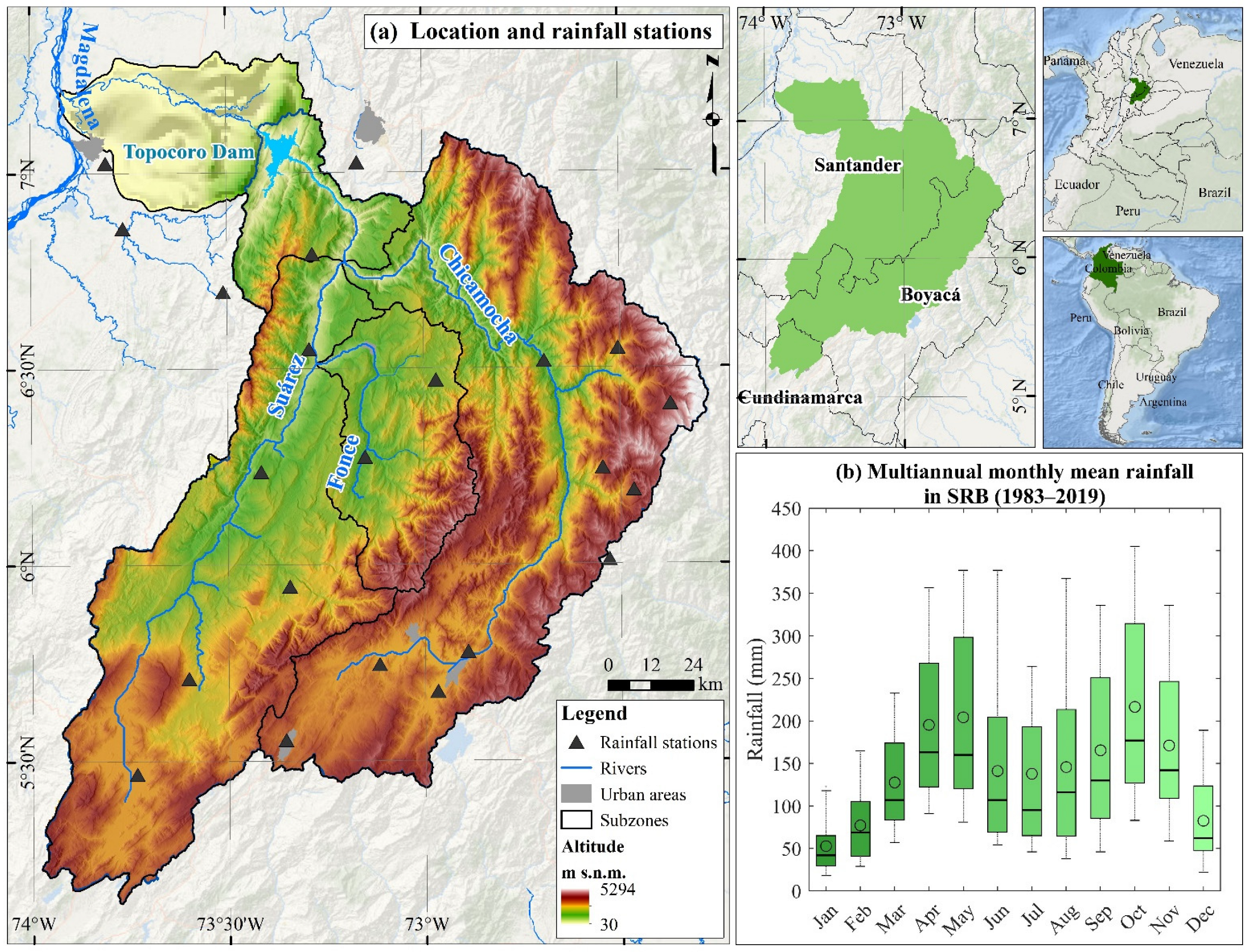
2.1. Study Area

The analyses were carried out in the SRB, covering 23,000 km², the drainage area of which covers the departments of Boyacá (5%), Cundinamarca (42%), and Santander (53%), through the confluence of the Chicamocha, Fonce, and Suárez rivers, which mainly drain into the Topocoro dam of the Sogamoso hydroelectric station (Figure 1a). The Sogamoso Hydroelectric Project is located in the Santander department in the northeastern zone of Colombia. The dam is located in a narrow canyon, where the Sogamoso River crosses perpendicular to the Serrania de La Paz 75 km upstream of its confluence with the Magdalena River (the main river in Colombia). The basin is part of the Magdalena-Cauca Hydrographic Area and the Sogamoso Hydrographic Zone [40]. The Topocoro dam has a water mirror of approximately 70 km²; it is one of the largest dams in the country, with a storage capacity of 4800 million m³. The Sogamoso Hydroelectric Project has an installed capacity of 820 MW (about 10% of the country’s requirements), producing approximately 5053 GWh per year.

Regarding the annual cycle of monthly mean rainfall for the SRB, Figure 1b shows a bimodal cycle with maximums in April–May, reaching 200 mm per month, and a second peak in October, when rainfall averages 217 mm. The lowest rainfall periods occur from December to February (DJF), with values below 80 mm per month, and from June to August (JJA), with monthly average values of 140 mm [35,41]. According to Guzmán et al. [41], this bimodal regime is due to the strong influence of the northeasterly trade winds associated with the southern migration from the Atlantic branch of the Intertropical Convergence Zone. Furthermore, the mid-year dry season is less pronounced than in DJF due to the lower elevations of the Andes Mountain range in this zone, conferring a more significant influence of the moisture originating from the Pacific Ocean on rainfall during this time of the year.

2.2. Rainfall Dataset

We used monthly rainfall time series from 1982 to 2019, which included the twenty-three rainfall-gauge stations located in different zones in the SRB (Figure 1a), as provided by the Institute of Hydrology, Meteorology, and Environmental Studies of Colombia (available at https://www.datos.gov.co/Ambiente-y-Desarrollo-Sostenible/Cat-logo-Nacional-de-Estaciones-del-IDEAM/hp9r-jxuu/data (accessed on 15 May 2022). In accordance with the World Meteorological Organization’s guide to meteorological instruments and methods of observation [42], the database was previously subjected to a quality control scheme and a cleaning of erroneous or uncertain data, with less 10% missing data in the period from January 1982 to December 2019.

2.3. The Climate Hazards Group Infrared Precipitation with Stations (CHIRPS v.2.0)

The climate hazards group infrared precipitation with stations (CHIRPS) is a satellite product developed by the US Geological Survey and the Climate Hazard Group (CHG) at the University of California, Santa Barbara, produced by the above “ intelligent” integration technology through (1) CHG precipitation climatology, (2) CHG thermal infrared-based satellite precipitation estimate (CHIRP), (3) Tropical Rainfall Measuring Mission precipitation estimates, (4) atmospheric model precipitation fields from the National Oceanic and Atmospheric Administration (NOAA) Climate Forecast System version 2, and (5) in situ rainfall gauges [43,44,45,46]. CHIRPS has provided a rainfall dataset on daily, pentad (5-day), and monthly temporal scales since 1981, with an approximate spatial resolution of 0.05° (5.5 km) and near-global land coverage (50° N–50° S) [47,48]. In this study, we used the CHIRPS v.2.0 at a monthly scale with a resolution of 0.05° for the period from 1982 to 2019 in the region spanning the Colombian territory (14° N–5° S and 65°–80° W). The data are available at https://data.chc.ucsb.edu/products/CHIRPS-2.0/ (accessed on 17 May 2021).

The CHIRPS dataset was previously validated in Colombia by Funk et al. [43] and Urrea et al. [49], and in regions of the Colombian Andes, such as Medellín, by López-Bermeo et al. [50] and Nariño by Ocampo-Marulanda et al. [51]. We agree that CHIRPS represents a data source that preserves the main features of rainfall on monthly and annual scales. López-Bermeo et al. [50] and Ocampo-Marulanda et al. [51] reported that CHIRPS can be used to analyze the seasonal and interannual variability associated with ENSO, as well as spatial rainfall patterns for the studied regions, mainly in mountainous areas.

2.4. Oceanic and Atmospheric Data

Monthly SST data from the NOAA Extended Reconstructed SST V5 (ERSST v5) dataset [52] were used. The data are available from 1854 to the present, with a horizontal resolution of 2° latitude by 2° longitude. The data are available for download from NOAA’s website (https://psl.noaa.gov/data/gridded/data.noaa.ersst.v5.html (accessed on 15 May 2022). We used the 1982–2019 period between 60° N–60° S and at all longitudes for the present work. Prior to the anomaly calculation, long-term trends (1901–2019) at each grid point were removed using the least-squares method. Afterward, the standardized seasonal anomaly time series were calculated considering the means and standard deviations for the 1982–2019 period.

Furthermore, we used the Oceanic Niño Index (ONI) derived from the NOAA Climate Prediction Center, measured as the 3-month running mean of the ERSST.v5 SST anomalies in the Niño 3.4 region (5° N–5° S and 120°–170° W) (available at https://www.cpc.ncep.noaa.gov/products/analysis_monitoring/ensostuff/ONI_v5.php (accessed on 15 May 2022).

The Chocó Jet (CJ) index, defined as the 925 hPa zonal wind anomalies averaged along 80° W and between 2° N and 7° N, was constructed as in several previous studies [9,53,54]. The Caribbean low-level jet (CLLJ) resides over the Caribbean Sea throughout the year [9,53,55]. We used the 925 hPa zonal wind anomalies in the region of 12.5° N–17.5° N, 80° W–70° W for the CLLJ index. To calculate these indices, we use the zonal winds (u) at 925 hPa during the 1982–2019 period derived from ERA5 reanalysis [56,57]. Data are provided on a regular latitude–longitude grid of 0.25°, representing available monthly mean data on pressure and individual levels (https://cds.climate.copernicus.eu/cdsapp#!/search?type=dataset (accessed on 21 September 2022)).

2.5. Standardized Precipitation Index and Principal Component Analysis

The monthly rainfall time series of the 23 stations in the SRB were transformed to the SPI. The SPI was designed by Mckee et al. [32] to determine whether there are deficits or excess rainfall in a region at a given time compared with normal conditions. The SPI is considered the most reliable index for measuring the intensity, duration, and spatial extent of dry and wet conditions [58]. It is an excellent tool for research on spatial analysis, as it removes the temporal effects of various rainfall magnitudes [59,60,61,62].

This index was designed to quantify the rainfall deficit or excess at different time scales (generally from 1 to 24 months). For this research, the SPI was calculated for three accumulation periods: one-month (SPI1), three-month (SPI3, quarterly), and six-month (SPI6, semiannual) periods. These time series of SPI were constructed through a moving sum adjusted to the gamma distribution, which is the best-fitted distribution with rainfall time series [63]. The gamma probability density function is:

$$g\left(x\right)=\frac{x^{\propto -1} e^{-\frac{x}{\beta }}}{{\beta }^{\alpha }\mathsf{\Gamma }\left(\alpha \right)}\hspace{1em}\mathrm{for}x>0$$

(1)

where $x$ is rainfall data, $\alpha$ is a shape parameter, $\beta$ is a form parameter, and $\mathsf{\Gamma }\left(\alpha \right)$ is the complete gamma function. According to the method of maximum likelihood, $\alpha$ and $\beta$ are:

$$\widehat{\alpha }=\frac{1}{4A}\left(1+\sqrt{1+\frac{4A}{3}}\right)$$

(2)

$$A=\ln \left(\overline{x}\right)-\frac{\sum \ln \left(x\right)}{n}$$

(3)

$$\widehat{\beta }=\frac{\overline{x}}{\widehat{\alpha }}$$

(4)

where $\overline{x}$ is the mean of rainfall time series, and $n$ is the rainfall observation number. In the above equations, precipitation $\left(x\right)$ must be greater than zero. This criterion is not usually met, especially when drought is under study. The cumulative probability becomes:

$$H\left(x\right)=q+\left(1-q\right)G\left(x\right)$$

(5)

where $G\left(x\right)$ is the cumulative probability of gamma when $g\left(x\right)$ is integrated with respect to $x$; and $q$ is the probability of no rainfall, which is calculated using $q=m/n$, where $m$ is the number of times at which the rainfall was zero in a temporal sequence of data and $n$ is the rainfall observation number in a sequence of data. The SPI is calculated based on the following equation according to Lloyd-Hughes and Saunders [64] and Zhang et al. [65]:

$$SPI=\left\{\begin{array}{c}-(t-\frac{c_0+c_{1}t+c_2{t}^2}{1+d_{1}t+d_2{t}^2+d_3{t}^3}\\ +(t-\frac{c_0+c_{1}t+c_2{t}^2}{1+d_{1}t+d_2{t}^2+d_3{t}^3}\end{array}\right\}\begin{array}{c}0<H\left(x\right)\le 0.5\\ 0.5<H\left(x\right) \le 1.0\end{array}$$

(6)

Furthermore, the expression $t$ is defined as:

$$t=\left\{\begin{array}{c}\sqrt{ln\frac{1}{{\left(H\left(x\right)\right)}^2}}\\ \sqrt{ln\frac{1}{{\left(1-H\left(x\right)\right)}^2}}\end{array}\right\}\begin{array}{c}, 0<H\left(x\right)\le 0.5\\ , 0.5<H\left(x\right) \le 1.0\end{array}$$

(7)

The constant values are: $c_0=2.515517, c_1=0.802853, c_2=0.010328, d_1=1.432788, d_2=0.189269$, and $d_3=0.001308$.

The main characteristic allows for monitoring of the drought/wetness with the normalization of the rainfall, with an average of 0 and a standard deviation of 1. Negative values less than or equal to –1.0 represent droughts, and positive values greater than or equal to 1.0 indicate that rainfall has been higher than the historical average. The classification based on SPI is extremely wet (2.0 or more), severely wet (1.5 to 1.99), moderately wet (1.0 to 1.49), normal (0.99 to −0.99), moderate drought (−1.0 to −1.49), severe drought (−1.5 to −1.99), or extreme drought (–2.0 or less).

Once the SPIs were obtained at the three selected scales for the 23 stations, principal component analysis (PCA) was carried out to reduce the dimensionality of the dataset into a smaller number of representative components (PCs) and provide the spatial and temporal variability patterns, as well as their importance [66,67]. PCA was performed separately for each SPI scale, generating the standardized time series or PCs, the eigenvalues or percentages of variance explained for each mode, and the eigenvectors or empirical orthogonal functions, which indicate the spatial pattern associated with each PC. A more detailed explanation of the PCA is provided by Lorenz [67], Björnsson and Venegas [66], and Wilks [68]. In this study, only the first principal component of each SPI was used to compare the most representative climate variability at multiple scales, which explains the maximum possible variance of the monthly, quarterly, and semiannual datasets.

2.6. Wavelet Analysis

In order to determine the dominant components of the SPI variability in the SRB, wavelet analysis was used [69]. Wavelet analysis allows the decomposition of a time series into different levels of time-frequency resolution; we applied this method to the PC1 of the SPI on a monthly scale. Computational procedures of the wavelet analysis used here are those described by Torrence and Compo [69] and Grinsted et al. [70]. The Morlet wavelet used in this study is a complex exponential modulated by a Gaussian function ($\psi \left(t\right)=e^{i{\omega }_0\eta }{e}^{-{\eta }^2/2}$, where $\eta =t/s$, $t$ is the time, $s$ is the wavelet scale according to time $\left(s=2/\partial t\right)$, and ${\omega }_0$ is the nondimensional frequency) [69]. The wavelet function of each scale (s) is normalized by $s^{-1/2}$ to obtain the unit energy. For a given scale ($s$), the global wavelet power (GWP) is the mean time expressed by Torrence and Compo [69]:

$$\overline{W^2}= \frac{1}{N} {{\displaystyle \sum }}_{n=0}^{N-1}{\left|W_n\left(s\right)\right|}^2$$

(8)

According to the procedures described by Torrence and Webster [71], the relationship between the monthly SPI-PC1 and ONI was investigated by wavelet coherence (WTC) analysis by calculating the cross-wavelet spectrum (XWT) and the coherence phase difference of the wavelets. The XWT of two time series (X(t) and Y(t)) is defined as: $W_t^{xy}=W_t^x{W}_t^y{}^{*}$, where * denotes complex conjugation. We further defined the XWT as $\left|W^{XY}\right|$. The XWT identifies the regions in time- frequency space where two time series show high common power. In addition, the WTC can measure the intensity of the covariance of the two series in the time-frequency space. The WTC of two time series ($W^X\left(t,s\right)$ and $W^Y\left(t,s\right)$) is defined as:

$$R_n^2\left(s\right)=\frac{{\left|S\left(s^{-1}{W}^{XY}\left(t,s\right)\right)\right|}^2}{S\left(s^{-1}{\left|W^X\left(t,s\right)\right|}^2\right) · S\left(s^{-1}{\left|W^Y\left(t,s\right)\right|}^2\right)}$$

(9)

where $S$ is a smoothing operator; $W^{XY}\left(t,s\right)=W^X\left(t,s\right)W^{Y*}\left(t,s\right)$ is the cross-wavelet spectrum; and $R_n^2$ can range from 0 to 1, with 0 indicating no correlation between the two series and 1 indicating a perfect correlation. Monte Carlo methods were used to estimate the statistical significance of the wavelet analysis and wavelet coherence [70,71].

Once the main modes of variability of the monthly SPI PC1 and the different scales of variability in which it is related to the ONI were obtained, wavelet analysis was used as a bandpass filter to reconstruct the time series, and the oceanic and atmospheric anomalies were used as the sum of the real part of the wavelet transform in an interval of $j_1$ and $j_2$ [69]:

$$x_n^{\prime }= \frac{\delta j\delta t^{1/2}}{C_{\delta }{\psi }_0\left(0\right)} {{\displaystyle \sum }}_{j=j_1}^{j_2}\frac{\Re \left\{W_n\left(s_j\right)\right\}}{s_j^{1/2}}$$

(10)

where ${\psi }_0\left(0\right)$ is a factor that removes the energy scaling, $s_j^{1/2}$ converts the wavelet transform to an energy density, and $C_{\delta }$ is a constant (for Morlet, $C_{\delta }=0.776$).

The scales selected for this filtering will be presented in the Results and Discussion section, where we will discuss the role of the interaction of multiple scales of variability in rainfall in the SRB and, in general, in the Colombian region, which could be related to the duration and/or strengthening of ENSO events at different time scales of variability. Box plots of the temporal evolution of SPI at the 23 stations in the SRB region during the ENSO events selected and filtered on the obtained scales of variability were also produced.

3. Results and Discussion

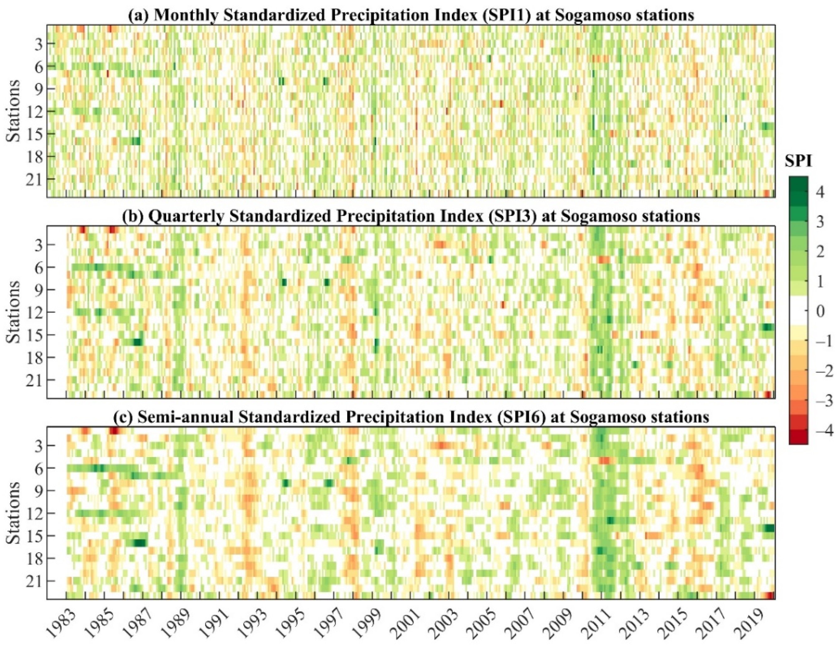
3.1. Standardized Precipitation Index

Figure 2 shows the temporal evolution of SPI1, SPI3, and SP6 for the 23 stations in the SRB, where a high variability in the frequency of monthly SPI is observed, whereas on the semiannual scale, there is a low variability of SPI. This result shows that some regions can respond to wet and dry conditions on different time scales, as noted by Cerón et al. [36], who showed that ENSO modulates rainfall in southwestern Colombia (Cali city) at interannual to decadal scales, with changes in equatorial Pacific SST occurring 6 to 18 months before wet or dry conditions in that region. Vicente-Serrano et al. [60] also pointed out a differentiation of the persistence of dry conditions in America and Eastern Europe due to the multiple timescales of variability involved, linked to ENSO on shorter timescales (1 to 3 months); the effects in South Africa, Australia, and southeastern Asia were evident a few months later and on longer timescales (6 to 12 months).

For a more consistent analysis of SPI variability and to improve our understanding of the multiple scales of variability that can affect the study area, we applied PCA for SPI1, SPI3, and SPI6 for the 23 SRB stations. The PCA analyses show that the dominant mode for each scale present an explained variance of 37% for SPI1, 40% for SPI3, and 43% for SPI6. Figure 3 shows the time series of PC1 for the three selected SPI scales. The results show that wetness and dryness changes are more evident at the shorter time scales (SPI1 and SP3). Nevertheless, SPI6 smooths the series and has fewer fluctuations (Figure 3c), and SPI6 allows for typification of common events for most stations, such as the wet periods of 1988–1989, 1995–1996, 1998–2000, 2010–2012, 2016–2017, and 2017–2018, and the dry periods of 1991–1992, 1997–1998, 2002–2003, 2009–2010, and 2014–2016; these periods are in agreement with those classified by NOAA as La Niña and El Niño events, respectively.

An important feature noticeable in the PC1 of SPI3 and SPI6 (Figure 3b,c) is the persistence of some anomalous rainfall events in the SRB for more than two years, consistent with current reports of multiyear ENSO events [7,19,72,73]. In this regard, a rainfall deficit in the SRB is observed from 2014 to 2016, coincident with the multiyear 2014–2016 El Niño event. According to Kim and Yu [74], the extreme El Niño of 2015–2016 was preceded by a weak El Niño event during 2014–2015, which could indicate that the extreme El Niño of 2015–2016 was part of a multiyear event, in contrast to the 1997–1998 extreme El Niño event that was preceded by the 1995–1996 La Niña event.

Moreover, the PC1 also shows two persistent excess rainfall events: a first event between 1998 and 2000 and a second event between 2010 and 2012, which coincide with the multiyear La Niña events discussed by Iwakiri and Watanabe [18] and Lopes et al. [7]. An important feature of these events is that they were immediately preceded by El Niño events—in this case, the 1997–1998 and 2009–2010 periods, respectively, consistent with [18,75,76]. These events are reflected in the rainfall deficits in the SRB presented in Figure 3c.

These results confirm ENSO as the dominant climate phenomenon in the tropical ocean that affects global climate and weather conditions in the SRB. However, although the relationship between rainfall deficits and excesses across the SPI in the SRB is consistent with ENSO events, some authors point out that multiple scales of variability, including biennial to decadal scales of ENSO [77,78], may act to maintain the multiyear events described above. In the next section, we explore the dominant modes of SPI variability in the SRB and the multiple scales of ENSO relationships.

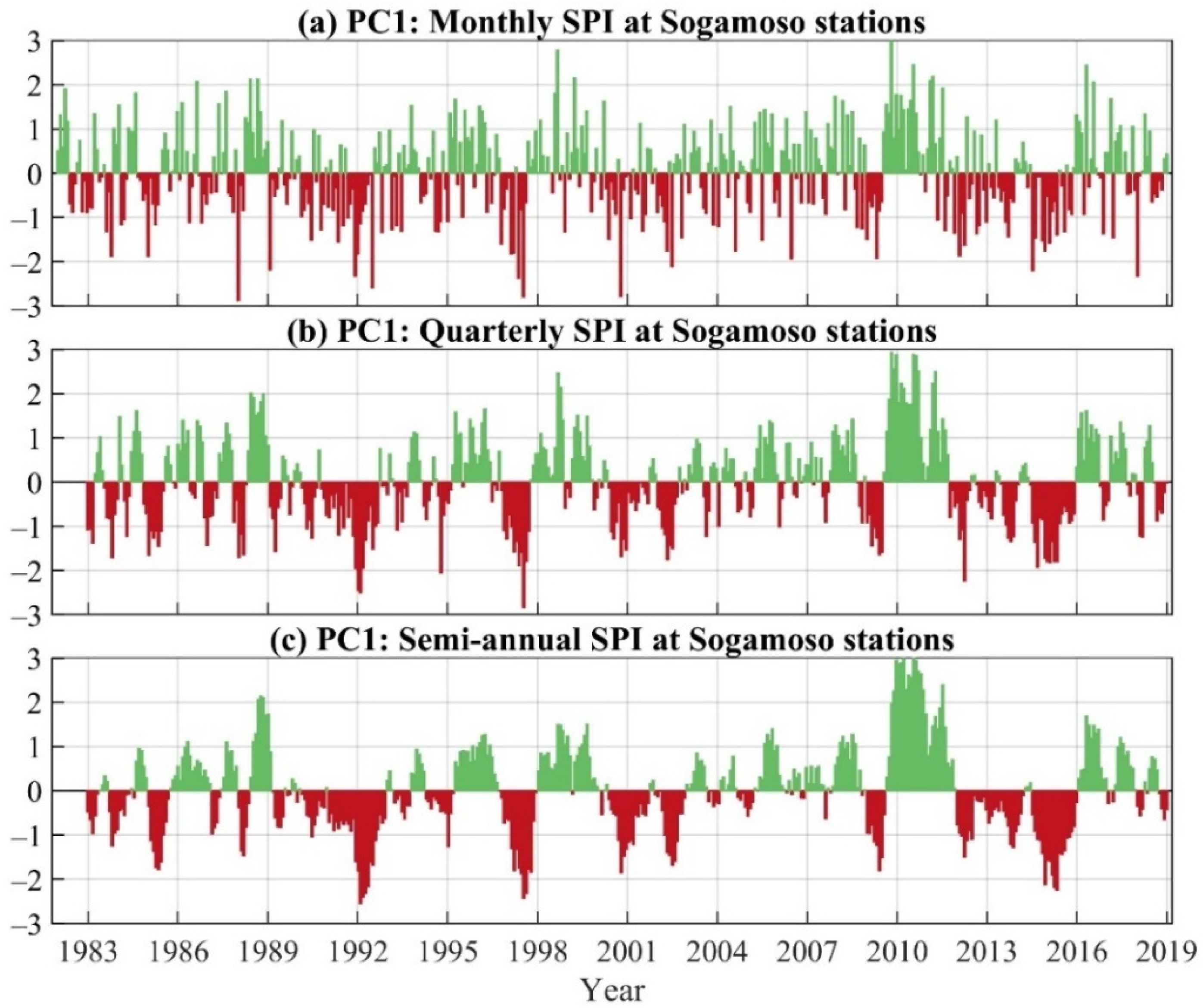
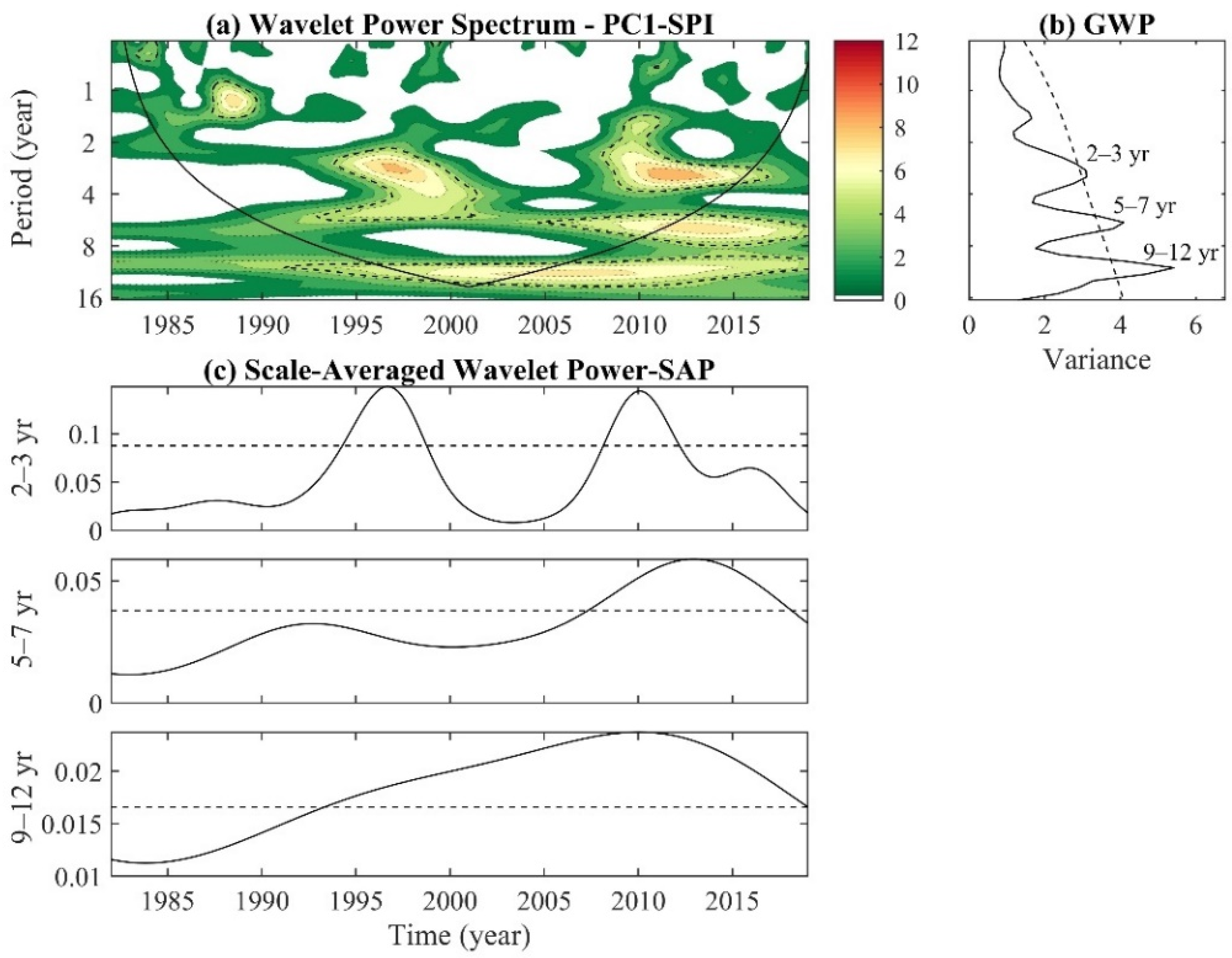
3.2. Time-Frequency Variations of the SPI

The wavelet analysis of the monthly PC1 time series of the SPI for the SRB shows high wavelet power on the 2–3-year quasi-biennial time scales from 1994 to 2002 and 2008 to 2015 (Figure 4a). High power was detected on the 5–7-year interannual time scale, mainly from 2005 onwards, and on the quasi-decadal time scale of 9–12 years appears after the 1990s (Figure 4a,b). The scale-averaged wavelet power (SAP; Figure 4c) corresponding to the three significant peaks found in the global wavelet power (Figure 4b) are also displayed. In general, the PC1 of SPI1 showed significant SAP values (in variance units) for the 2–3-year scale during the 1994–1999 and 2008–2012 periods (Figure 4c). For the 5–7-year scale, there are significant SAP values starting in 2007, peaking in 2012, and decaying in 2019. The SAP series for the 9–12-year scale records significant values starting in 1994, peaking in 2010, and declining by 2019.

These results confirm that the SPI for the SRB responds to multiple scales of variability, which, interacting with each other, could be relevant to the persistence and intensity of some rainfall events that occurred during the analysis period. In the next section, we discuss how these scales of variability are related to ENSO through the XTC and WTC between the monthly SPI PC1 series and the ONI index.

3.3. Linkage between SPI and ENSO Events

Figure 5 shows the XWT and WTC between the PC1 series of the SPI in the SRB and the ONI. The XWT shows common periods with a significant power spectrum on interannual (2 to 7 yr) and quasi-decadal (9 to 12 yr) time scales in the antiphase (Figure 5a). However, on the interannual scale, it is important to note that the XWT and WTC are not homogeneous throughout the study period (Figure 5a,b). On the 2–3-year scale, common periods with significant power spectra span over longer periods from 1994 to 2002 and from 2008 to 2015; on this scale, the 180° lag indicates that the positive (negative) values have a synchronous relationship with the La Niña (El Niño) mature phase of the events. Figure 6a shows the ONI and SPI series filtered at the 2–3-year scale; overall, there is strong synchrony between the series in the 1988–2000 and 2006–2015 periods, with a weak synchrony in the 2002–2006 period, supporting the weak relationship presented by the XWT in this period (Figure 5a).

Moreover, the relationship of the series on the 5–7-year scale is strongest from 1995 to 2011, with the WTC showing a phase difference of −160° between 1995 and 2005 and −90° between 2007 and 2011 (Figure 5b). The −160° phase difference indicates that the maximum (minimum) SPI occurs 3 to 5 months before the minimum (maximum) peak of the ONI, that is, in the development phase of a La Niña (El Niño) event. On the other hand, the −90° phase difference indicates that maximum (minimum) SPI preceded the mature La Niña (El Niño) phase by approximately 15–21 months. Accordingly, the filtered series on the same scale (Figure 6b) show an increase in the lag between ONI and SPI after 2000.

Additionally, the XWT shows a higher energy relationship between the SPI and ONI PC1 series on the 9–12-year quasi-decadal scale for the 1994–2012 period (Figure 5a). The WTC displayed considerable coherence on the quasi-decadal scale from 1995 to 2005, with a −135° phase difference (Figure 5b), which indicates that maximum (minimum) SPI preceded the mature La Niña (El Niño) phase by approximately 13–18 months, as reflected in the series filtered at the quasi-decadal scale in Figure 6c.

Therefore, it is possible to indicate that the amplitude and dominant modes of variability between ENSO and SPI have shifted over time. Consequently, the interaction between quasi-biennial and quasi-decadal scales of variability plays a differential role in the configuration and prolongation of intense rainfall events in the SRB. Although the time series spans 38 years, it was sufficiently long to resolve the 9–12-year scale variability so that three ONI peaks associated with La Niña occurred in 1988, 1999, and 2010 (Figure 6c). Among these events, the last two observed in Figure 6c tend to be in phase with 2–3-year La Niña events (1998–2000 and 2010–2011; Figure 6a). On this basis, in the following sections, we compare the influence of these scales of variability on the 1998–2000 and 2010–2012 multiyear La Niña events and their differential effects on the prolongation of rainfall excesses across Colombia, particularly in the SRB.

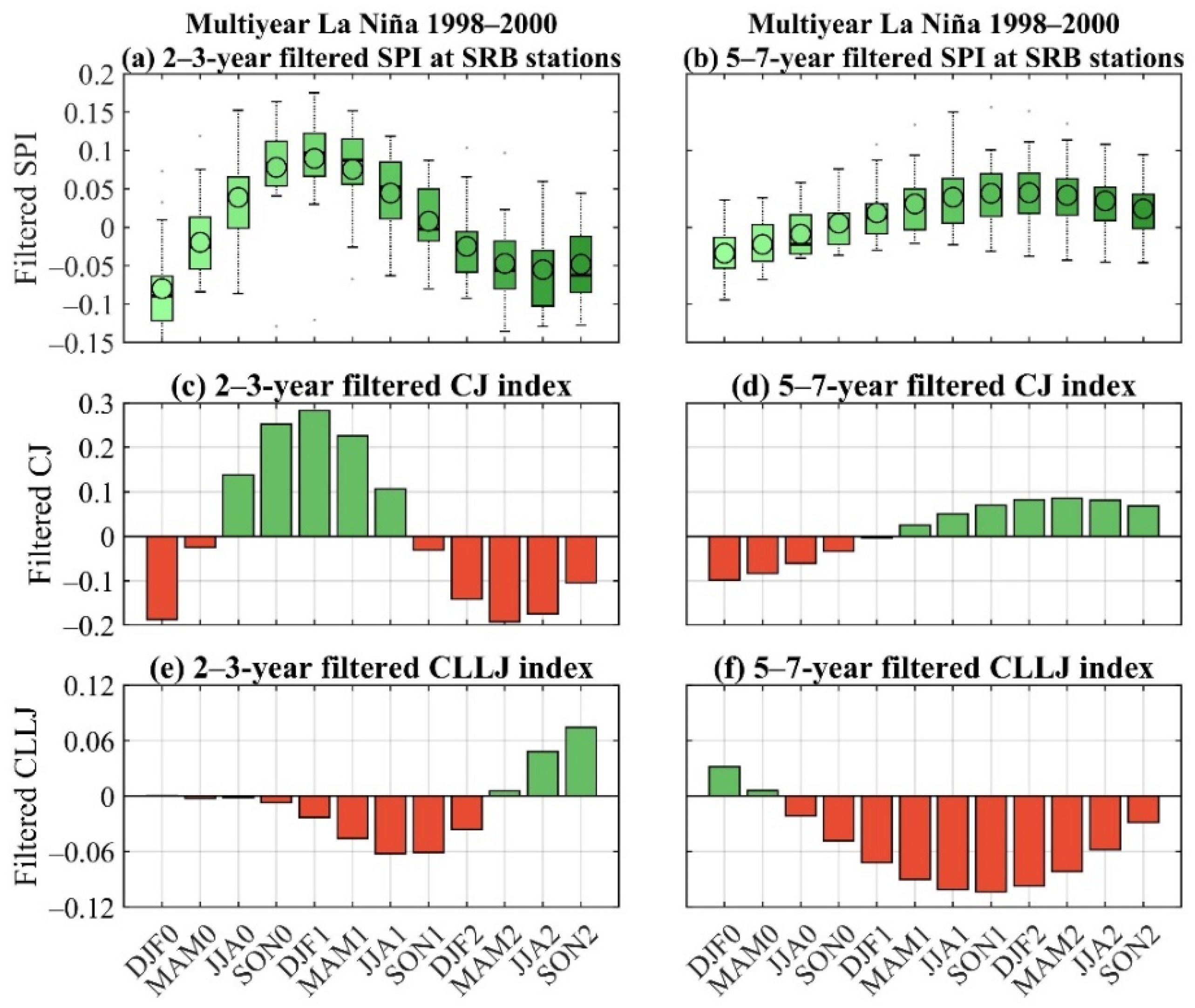
3.4. Quasi-Biennial and Interannual Scales of the 1998–2000 La Niña Event

Seasonal SST anomalies filtered at quasi-biennial (2–3-year) and interannual (5–7-year) scales during 1998–2000 show distinct patterns between them (Figure 7), confirming a differential role in the configuration of the La Niña event and its duration for more than one year.

On the quasi-biennial scale (Figure 7a–l), the emergence of warmer conditions over the equatorial Pacific was noted during the first half of 1998 (Figure 7a,b), surrounded by negative anomalies in the subtropical Pacific, extending over the Australasian region, in accordance with the 1997–1998 El Niño event. Afterward, a cooler central tropical Pacific event started to develop in SON 1998, and La Niña conditions prevailed until JJA 1999 (Figure 7d–g). La Niña conditions weakened in the next quarter and disappeared in early 2000 (Figure 7i). Warmer conditions over the equatorial Pacific have prevailed since MAM 2000 (Figure 7j–l). On the interannual scale (Figure 7m–x), warming was observed starting in DJF 1998, which weakened in DJF 1999. The negative SST anomalies prevailed in the western tropical Pacific region north of the equator starting in DJF 1998 and extended in a southwest–northeast band towards the North American coast from DJF 1999 until SON 1999 (Figure 7q–t). During 2000 (Figure 7u–x), negative SST anomalies over the tropical Pacific persisted throughout the year and extended meridionally over the western coast of the Americas. Negative SST anomalies over the tropical North Atlantic (TNA) also developed starting in SON 1999 and over the Indian Ocean starting in DJF 1999 (Figure 7q–x).

Accordingly, the SPI filtered at quasi-biennial scales for the Colombian territory (Figure 8a–l) showed dry conditions throughout DJF and MAM of 1998 over the Andean, Caribbean, and Pacific regions; wet conditions appeared in northern Colombia from JJA 1998 and extended to the Andean and Pacific regions until JJA 1999, later weakening in SON 1999; and dry conditions were noted during most of 2000, mainly in northern Colombia. The SPI filtered to the interannual scale (Figure 8m–x) showed normal conditions over most of Colombia during 1998 (Figure 8m–p), whereas wet conditions prevailed during 1999 and 2000 over the Caribbean, Andean, and Pacific regions (Figure 8q–x), consistent with the La Niña SST patterns displayed in Figure 7q–x.

Therefore, the spatiotemporal evolution of SST anomalies on quasi-biennial and interannual scales (Figure 7) played a differential role in the persistence of multiyear La Niña conditions in 1998–2000, as well as the persistence of rainfall over the Colombian territory (Figure 8). El Niño conditions were consistent between scales during the first half of 1998, showing stronger prevalence on the quasi-biennial scale. During the second half of 1998, weak El Niño conditions prevailed on the interannual scale, whereas cooling of the eastern and central equatorial Pacific occurred at the end of 1998 on the quasi-biennial scale. In 1999, a cooling of the central and eastern tropical Pacific (western tropical Pacific) prevailed on the quasi-biennial (interannual) scale, and during 2000, La Niña conditions were only observed on the interannual scale. Hence, we can conclude that the quasi-biennial scale variability promoted wet conditions (positive SPI) in the Caribbean, Andes, and Colombian Pacific from JJA 1998 to JJA 1999, whereas the interannual scale variability promoted intensification of these conditions during 1999 and contributed to their maintenance until the end of 2000.

Furthermore, the temporal evolution of the filtered SPI at the 23 SRB stations supports our findings for the 1998–2000 multiyear La Niña (Figure 9a,b). The box plot on the quasi-biennial scale shows an evolution from dry to wet conditions in 1998, with a peak of wetness in most SRB stations during 1999; neutral to dry conditions were observed in 2000. On the other hand, the box plot of the interannual scale shows a temporal evolution from normal conditions in 1998 to wet conditions between 1999 and 2000, reaching its highest peak of wetness between SON of 1999 and DJF of 2000 in most of the stations.

The SPI increase or decrease over the SRB and Colombia on these variability timescales is explained by the changes in the SST anomaly gradient over the tropical Pacific, the Caribbean Sea, and TNA (Figure 7), which consequently affected the circulation associated with the low-level jets (LLJ) from northern South America and played an important role in the moisture transport towards the Colombian region [38,39,53]. Figure 9c–f present the filtered CJ and CLLJ indices on the quasi-biennial and interannual time scales. On the quasi-biennial scale, the CJ showed an intensification from late 1998 to JJA 1999 (Figure 9c), consistent with the negative SST anomalies in the tropical Pacific during this period (Figure 7d–g), and a weakening throughout 2000 due to the warming of the surface waters in the eastern tropical Pacific (Figure 7i–l). Its intensification resulted in an increase in the SPI (Figure 8c–g and Figure 9a) due to the CJ moisture transport from the eastern Pacific Ocean to the continental region of Colombia during 1999. Meanwhile, quasi-biennial CLLJ was almost imperceptible during 1998 and very weak until the beginning of 2000 (Figure 9e), consistent with the positive-to-neutral SST anomalies in the Caribbean Sea observed during this period (Figure 7d–g). In agreement with Cerón et al. [53], a negative tropical Pacific–Caribbean SST gradient (SST_Pacific < SST_Caribbean; Figure 7d–h) strengthened the moisture transport from the Pacific to the Caribbean Sea and Colombia, increasing the rainfall over the Colombian territory and the SRB during 1998–1999 (Figure 8d–g and Figure 9a).

Moreover, on the interannual scale, the CJ weakened at the beginning of 1998 and strengthened during 1999–2000 (Figure 9d), whereas the CLLJ showed negative values starting in JJA 1998. In this regard, the 1999–2000 CJ did not intensify to the same extent as on the quasi-biennial scale during 1998 because the negative SST anomalies in the tropical Pacific occurred in the western region (Figure 7q–t). According to Yepes et al. [39] and Cerón et al. [27,79], CJ has stronger relationships with the eastern tropical Pacific; therefore, lower magnitudes of CJ are expected when SST anomalies occur in the central or western Pacific region. Nevertheless, the more pronounced weakening of the CLLJ (Figure 9f) permits the preservation of circulation from the Pacific Ocean towards the continent, supporting rainfall over Colombia (Figure 8q–x) and especially over the SRB during 1999–2000 (Figure 9b).

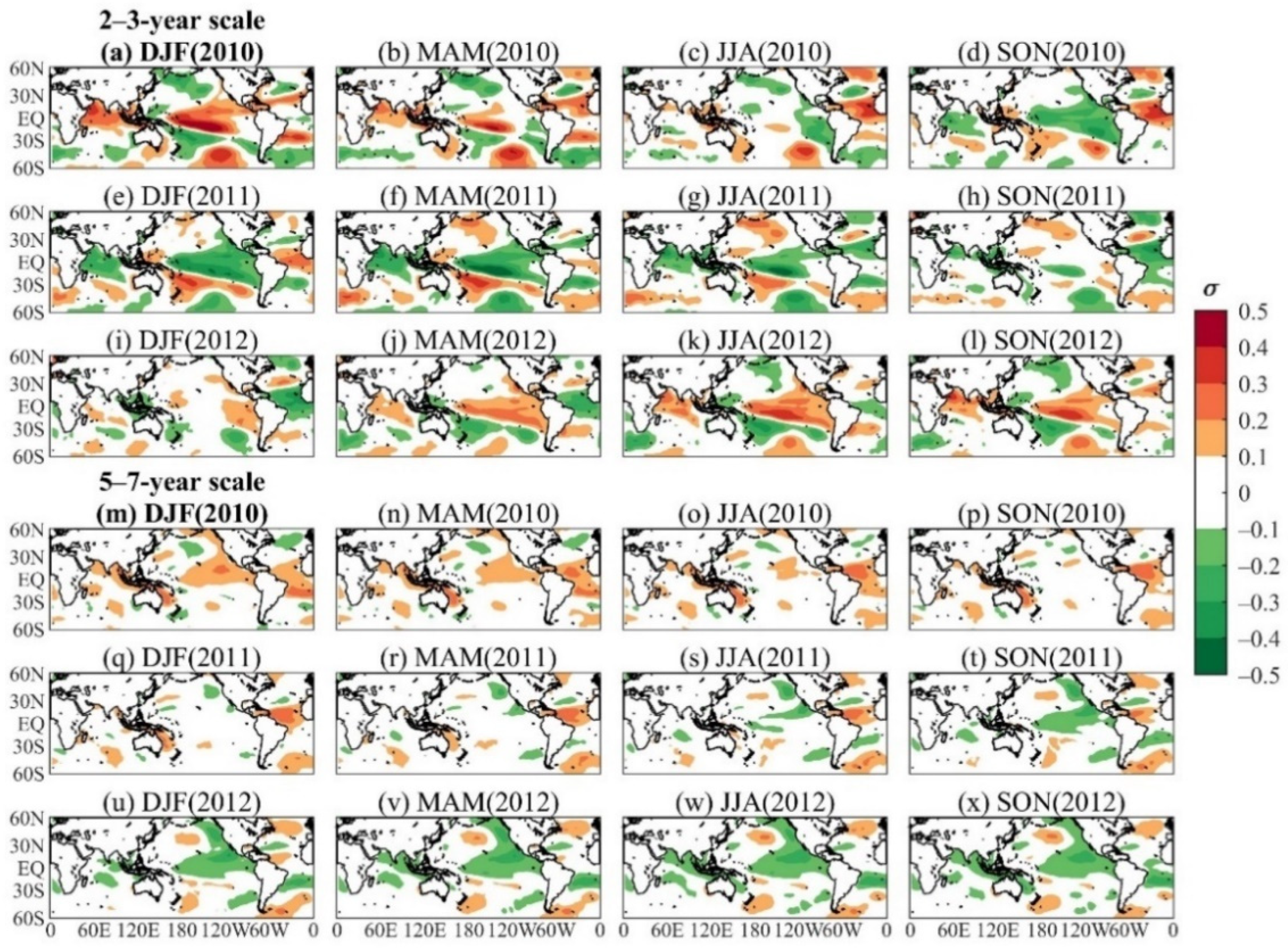
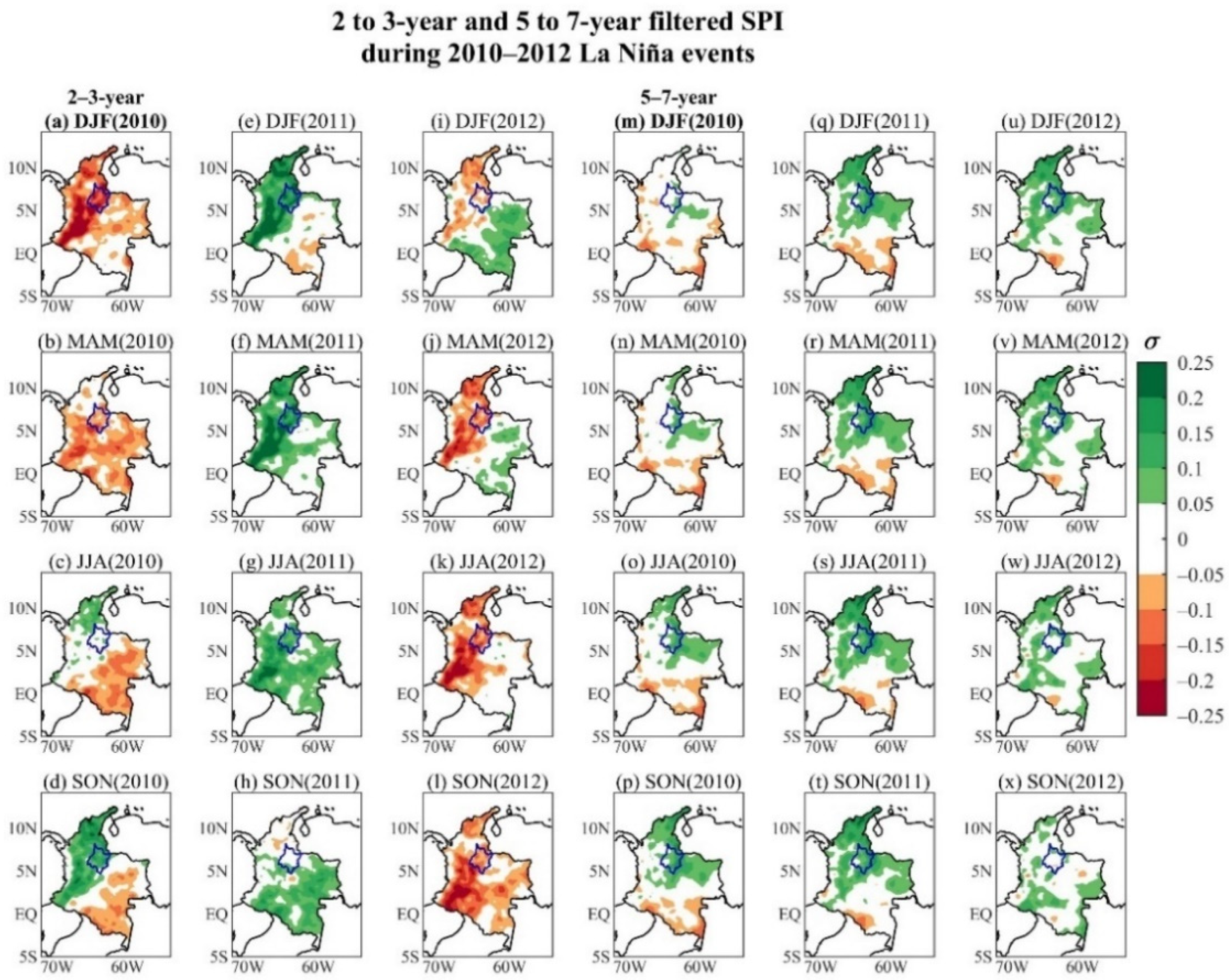
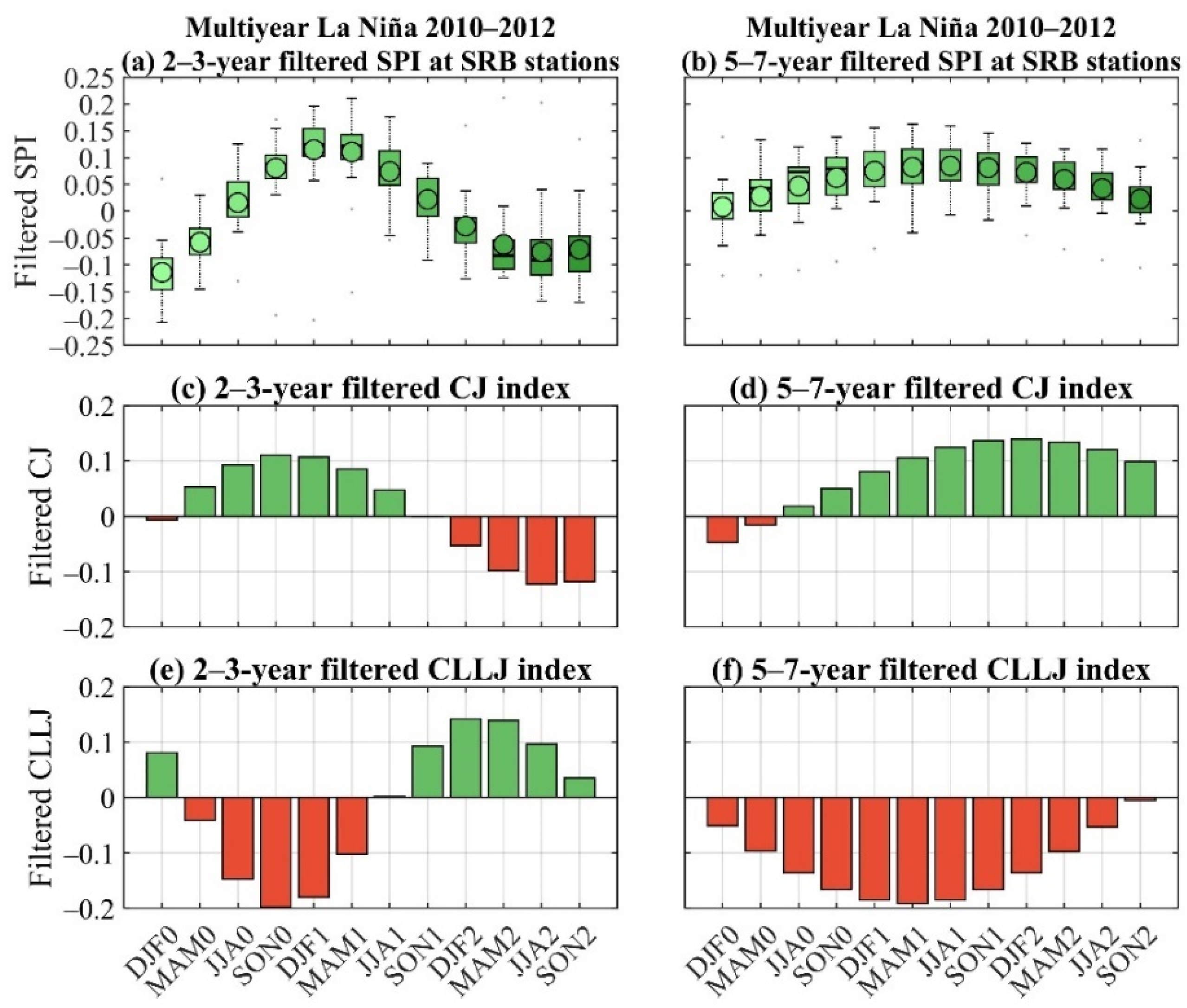
3.5. Quasi-Biennial and Interannual Scales of the 2010–2012 La Niña Event

During the 2010–2011 La Niña event, quasi-biennial SST anomalies indicated a warming of the central and eastern tropical Pacific in the first half of 2010, consistent with the 2009–2010 El Niño event (Figure 10a,b). During MAM 2010, negative SST anomalies were noted in the eastern Pacific along the coast of South America, extending and strengthening towards the central tropical Pacific starting in JJA 2010 before disappearing in SON 2011 (Figure 10c–g). During 2012, positive tropical Pacific SST anomalies extended from the coast of South and Central America during DJF into the central tropical Pacific in SON. Furthermore, warming of TNA occurred from DJF 2010 and persisted until DJF 2011, whereas negative anomalies in the same region prevailed from JJA 2011 to JJA 2012. Moreover, the interannual scale presents contrasting results to the quasi-biennial scale (Figure 10m–x). Positive SST anomalies were observed over TNA and the Caribbean from DJF 2010 to DJF 2012, whereas normal conditions prevailed over the tropical Pacific from JJA 2010 to JJA 2011. Thereafter, negative SST anomalies extended from the coasts of North and Central America to the central tropical Pacific starting in SON 2011 and remained throughout 2012, coupled with near-normal conditions over TNA and the Caribbean.

Consistent with the previous results, on the quasi-biennial scale, dry conditions were observed during the first half of 2010 over most of the Colombian territory, and wet conditions emerged over the Caribbean, Andean, and Pacific regions from JJA 2010 to JJA 2011 (Figure 11c–g), consistent with a La Niña SST pattern during this same period. In 2012, dry conditions prevailed in the same regions due to an El Niño SST pattern. In contrast, on the interannual scale (Figure 11m–x), wet conditions were noted over northeastern Colombia (where the SRB is located) starting in DJF 2010 and extending towards the Caribbean and Andean regions until JJA 2012, when they began to weaken.

In the same sense, the box plots of the SPI series for the 23 stations in the SRB and the LLJs filtered at quasi-biennial and interannual scales are consistent with the above-described results (Figure 12). On the quasi-biennial scale, an increase in SPI was observed from JJA of 2010 to JJA of 2011 (Figure 12a) due to a well-configured eastern tropical Pacific–Caribbean/TNA interbasin gradient (SST_Pacific < SST_{Caribbean/TNA}; Figure 10c–e), which strengthened the CJ and weakened the CLLJ from MAM of 2010 to MAM of 2011 (Figure 12c,e). During 2012, the SST anomaly gradient reversed (SST_Pacific > SST_{Caribbean/TNA}), producing a weakened CJ and a strengthened CLLJ, implying a reduction in ocean-to-continent moisture transport, increasing dry conditions over the SRB at the end of the event (Figure 12a). On the interannual scale, a persistence of wet conditions was observed at most stations over the SRB (Figure 12b), mainly linked to a negative SST gradient between the Pacific and the Atlantic (SST_Pacific < SST_{Caribbean/TNA}) during the whole period, which strengthened the CJ and weakened the CLLJ (Figure 12d,f).

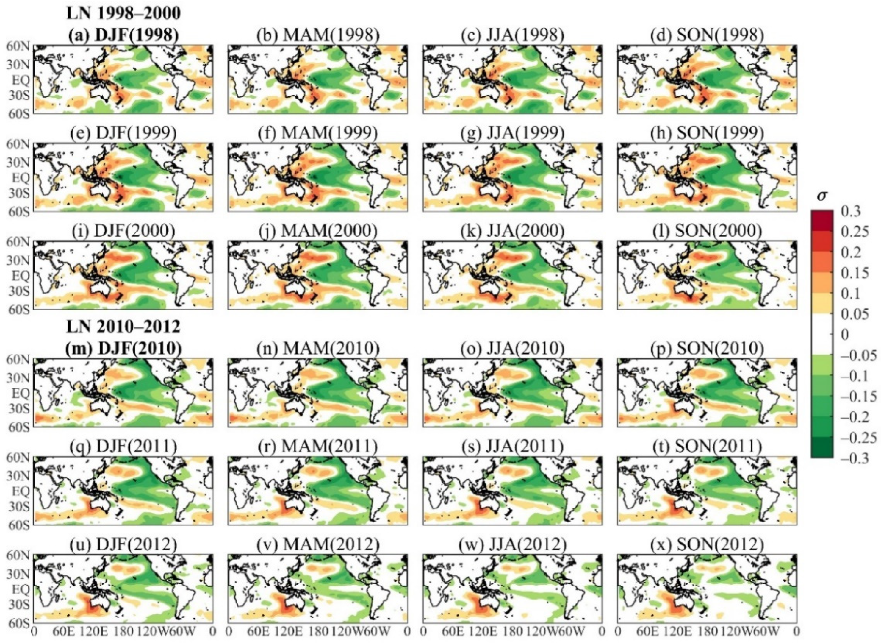
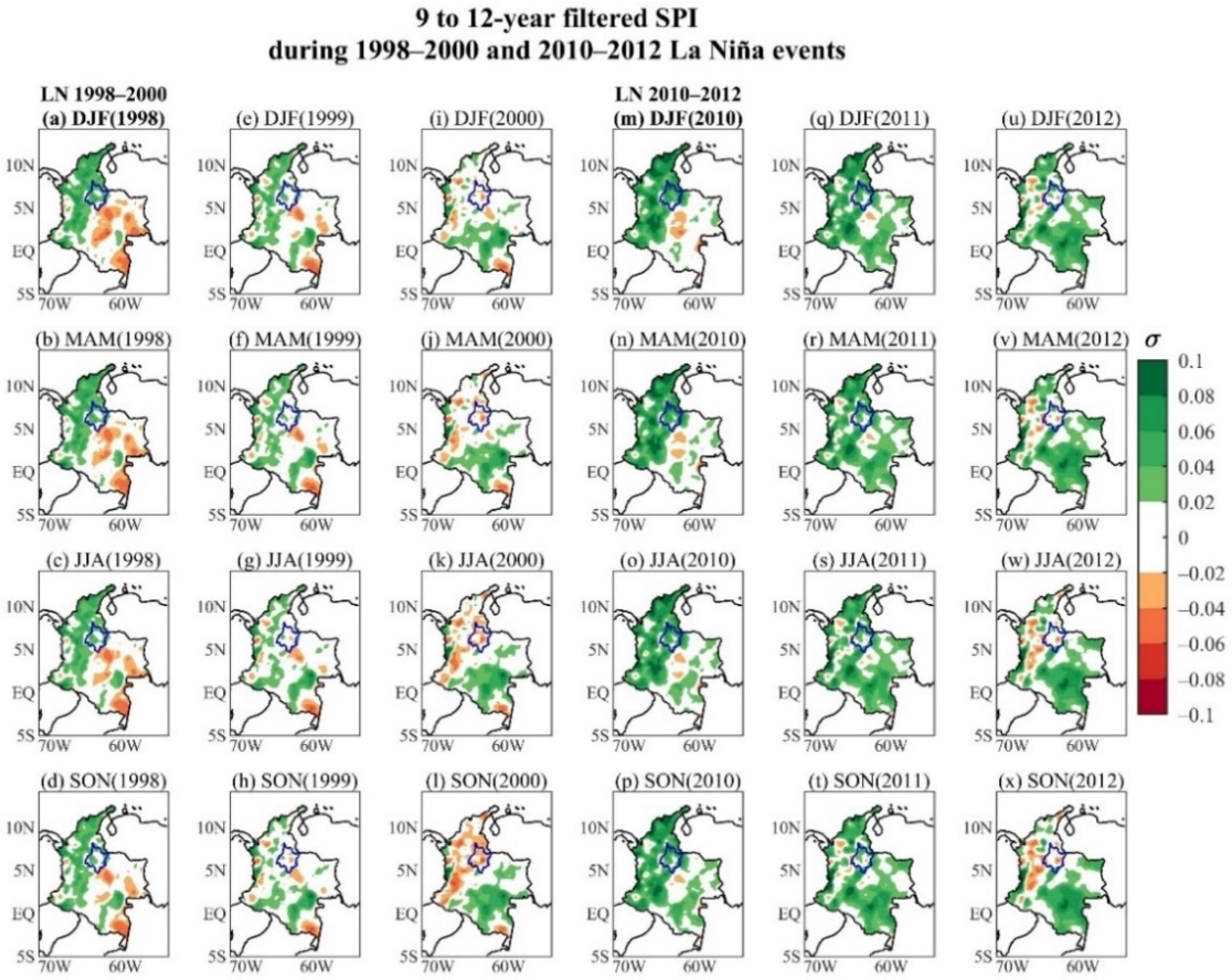
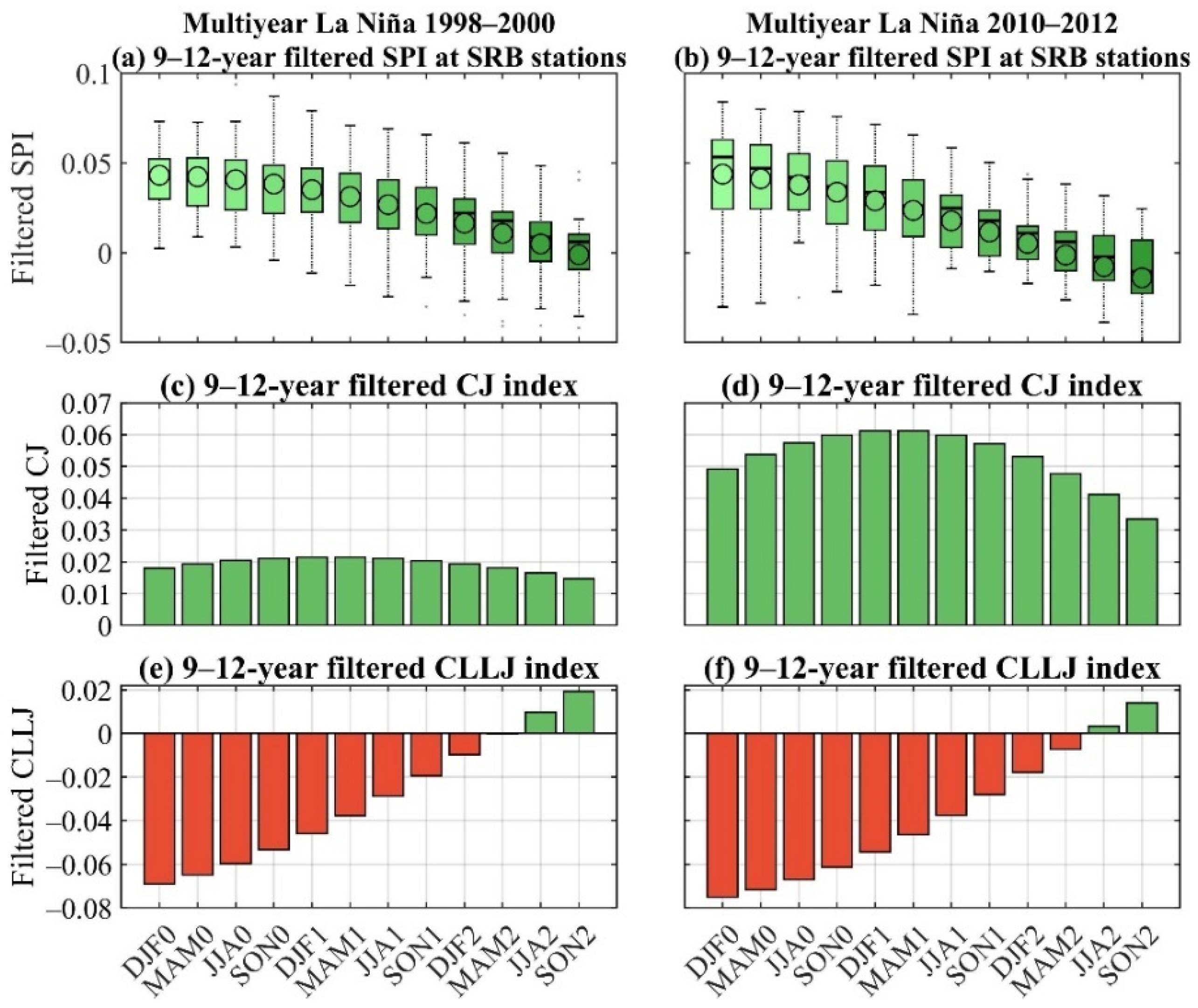
3.6. Quasi-Decadal Scales of La Niña Events

The above results show that the 1998–2000 and 2010–2012 multiyear La Niña events were the strongest in the SRB, as reflected by the power spectrum and the scale-averaged wavelet power shown in Figure 4a,c. Moreover, these two events occurred at the peak of the ONI on the 9–12-year scale (Figure 6c). However, their effects differed slightly due to a low-frequency modulation, as discussed below.

Seasonal SST and SPI anomalies were filtered on a quasi-decadal scale (9–12-year), and the 1998–2000 and 2010–2012 multiyear La Niña events are shown in Figure 13 and Figure 14. The SST indicates a cold phase of the Pacific decadal oscillation (CPDO) acting during the two events, characterized by an anomalous warming in the central North Pacific co-occurring with an anomalous cooling along the west coast of the Americas, as previously described by Mantua and Hare [80].

Nevertheless, significant changes were evident between the two events. According to Mantua and Hare [80] and Kayano et al. [81], during the 1998–2000 La Niña, the PDO was in its transitional phase from warm (WPDO, 1977–1998) to cold (CPDO, 2001–2015) conditions, resulting in weakly configured positive SST anomalies in the central North Pacific during 1998, which strengthened in the following two years (Figure 13a–l), whereas negative SST anomalies along the western coast of North America intensified by the end of 1998 and remained until the end of 2000. However, the eastern tropical Pacific in the 20° N–20° S band and between 120° W and the coast of South America exhibited warm-to-normal conditions throughout the event. Although normal conditions occurred over TNA and the Caribbean Sea, anomalous warming over the equatorial Atlantic was observed from DJF 1998 to JJA 2000.

The 2010–2012 La Niña event developed under conditions of the 2001–2015 CPDO, which intensified the La Niña effect over the tropical Pacific [82]. In this regard, Figure 13m–x show negative SST anomalies over most of the eastern and central tropical Pacific, exhibiting a strong meridional component during the first two years, coupled with anomalous warming of the central and western North Pacific; during 2012, this pattern weakened, and the negative anomalies noted in the equatorial Pacific between the coast of South America and 120° W weakened until reaching normal conditions.

Consequently, the SPI filtered at the quasi-decadal scale presented important differences between the 1998–2000 and 2010–2012 events (Figure 14). During 1998–2000 (Figure 14a–l), wet conditions occurred over the Caribbean region and the Andes during 1998, which weakened and dispersed in 1999, changing to dry conditions at the end of 2000, except for the southern region of the country. More extended and intense SPI wet conditions were observed during the 2010–2012 La Niña over most of the Colombian territory (Figure 14m–x), with greater intensity over the Caribbean, the Andes, and the Pacific region during 2010–2011. Afterward, wet conditions occurred over eastern Colombia, the west coast of the country, and the foothills of the eastern cordillera in the Colombian Andes, whereas dry-to-normal conditions prevailed in the Andes during the second half of 2012.

In the same sense, the SPI of the SRB stations filtered on a quasi-decadal scale (Figure 15a,b) shows the wettest conditions for the 2010–2012 La Niña event, when a more intense CJ on a quasi-decadal scale (Figure 15d) associated with a tropical Pacific anomalous cold during 2010–2011 (Figure 13m–t) allowed moisture transport from the ocean to the continent, in synchrony with a weakened CLLJ due to the normal-to-warm conditions in the equatorial Atlantic during 2010. The 1998–2000 La Niña event showed a CJ with magnitudes significantly lower than those of 2010–2012 (Figure 15c) due to the warm-to-normal conditions in the eastern tropical Pacific near the northwestern coast of South America, surrounded by negative anomalies over the central tropical Pacific (Figure 13a–l) and a weakened CLLJ due to the anomalous warming of the equatorial Atlantic throughout the period (Figure 15e). Consequently, wet conditions prevailed from early 1998 to near-normal conditions between 1999–2000 (Figure 15a), which were lower than those observed during 2010–2012.

4. Conclusions

In this study, we examined the spatiotemporal rainfall variations in the SRB through SPI and investigated its relationships at multiple scales of variability with ENSO from 1982 to 2019, such as its implications for the 1998–2000 and 2010–2012 multiyear La Niña events. The XWT and WTC results revealed that ENSO shared a similar common power with SPI at three scales of variability: (i) quasi-biennial (2–3 years) from 1994 to 2002 and from 2008 to 2015, with a synchronous relationship between the mature stage of La Niña (El Niño) events and the positive (negative) SPI values; (ii) interannual (5–7 years) from 1995 to 2005, with a lag of 3–5 months between the maximum of SPI and the minimum ENSO peak, and from 2007 to 2011, with maximum SPI preceding the minimum ENSO peak by approximately 15–21 months; and (iii) quasi-decadal (9–12 years) from 1995 to 2005, showing a lag of 13–18 months between the maximum SPI and the mature stage of La Niña. These results show that the relationships between SPI and ENSO have changed over time depending on the time scale, playing a differential role in the configuration and duration of intense precipitation events over the SRB, such as the 1998–2000 and 2010–2012 multiyear events.

Our analysis was based on the wavelet technique, which has the advantage of finding the variability scales with maximum local variances in time. In this sense, we can see that in the wavelet analysis for the PC1-SPI series, the quasi-biennial and interannual signals (2–3 years and 5–7 years, respectively) show maximum variances in the periods of 1995–2000 and onwards. Additionally, a longer time scale of 9 to 12 years (quasi-decadal) appears after the 1990s. The quasi-decadal signal reported in this study is consistent with the long SST time series analysis results reported by Silva et al. [83,84], showing that the signal becomes stronger after the 1970s, consistent with our XWT analysis results, where a more significant relationship in terms of energy is demonstrated between the PC1-SPI and ONI series on the quasi-decadal scale in the 1994–2012 period. Furthermore, two minima of the quasi-decadal oscillation (1999 and 2010) in the ONI series (Figure 6) are in-phase with the 2 to 3-year La Niña events (1998–2000 and 2010–2011). Based on this result and considering that the series were decomposed on different time scales with a wavelet-based filter, we can investigate how each scale of variability (quasi-biennial to quasi-decadal) individually contributes to the persistence of rainfall excess over the SRB in the 1998–2000 and 2010–2012 periods, even for the limited 1982–2019 period.

Further confirming the above, wavelet analyses were used to filter the seasonal anomalies of SST and SPI (in the Colombia region and for the rainfall stations within the SRB), as well as the CJ and CLLJ indices on the observed scales of variability. The most outstanding results were:

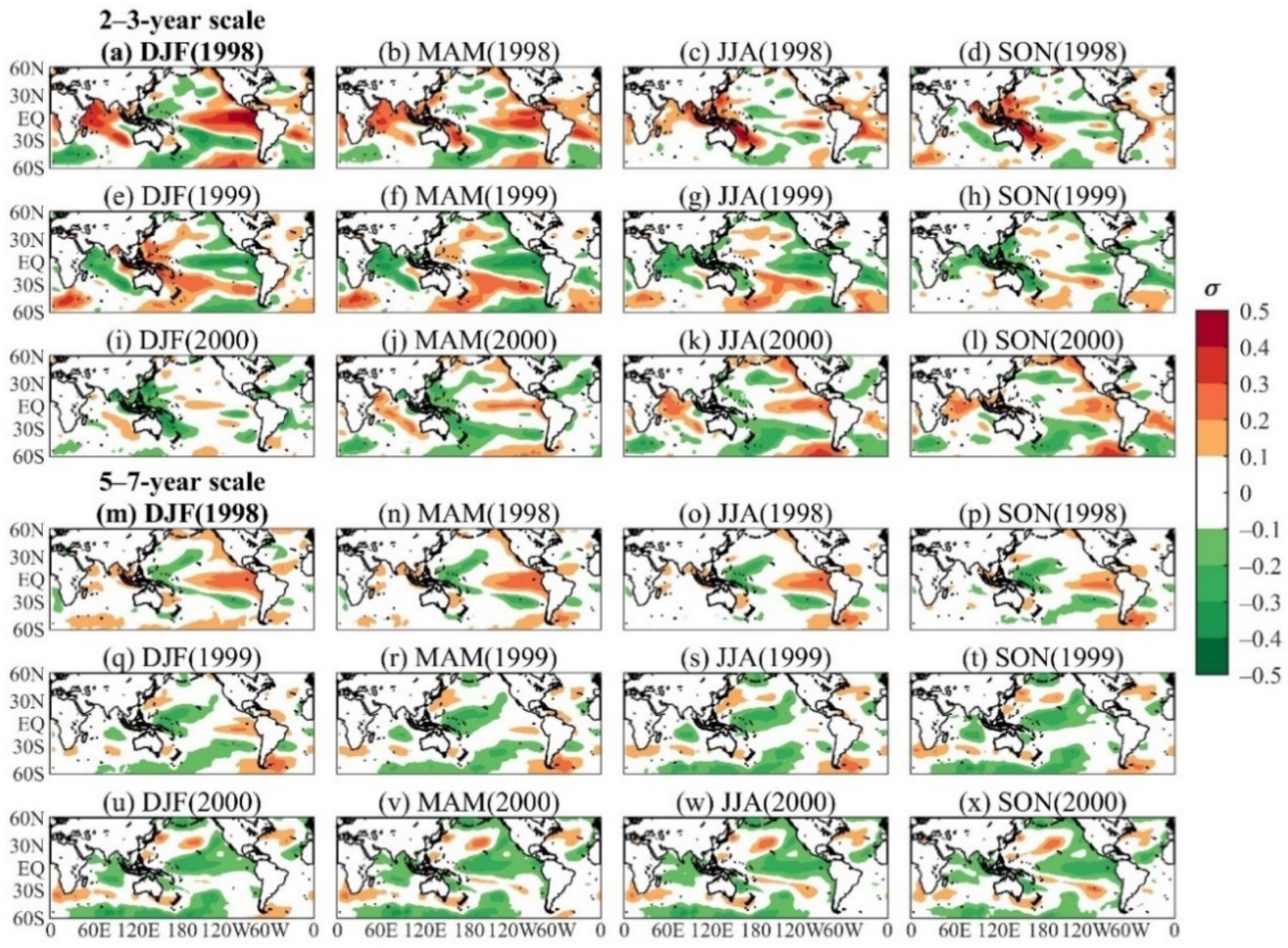
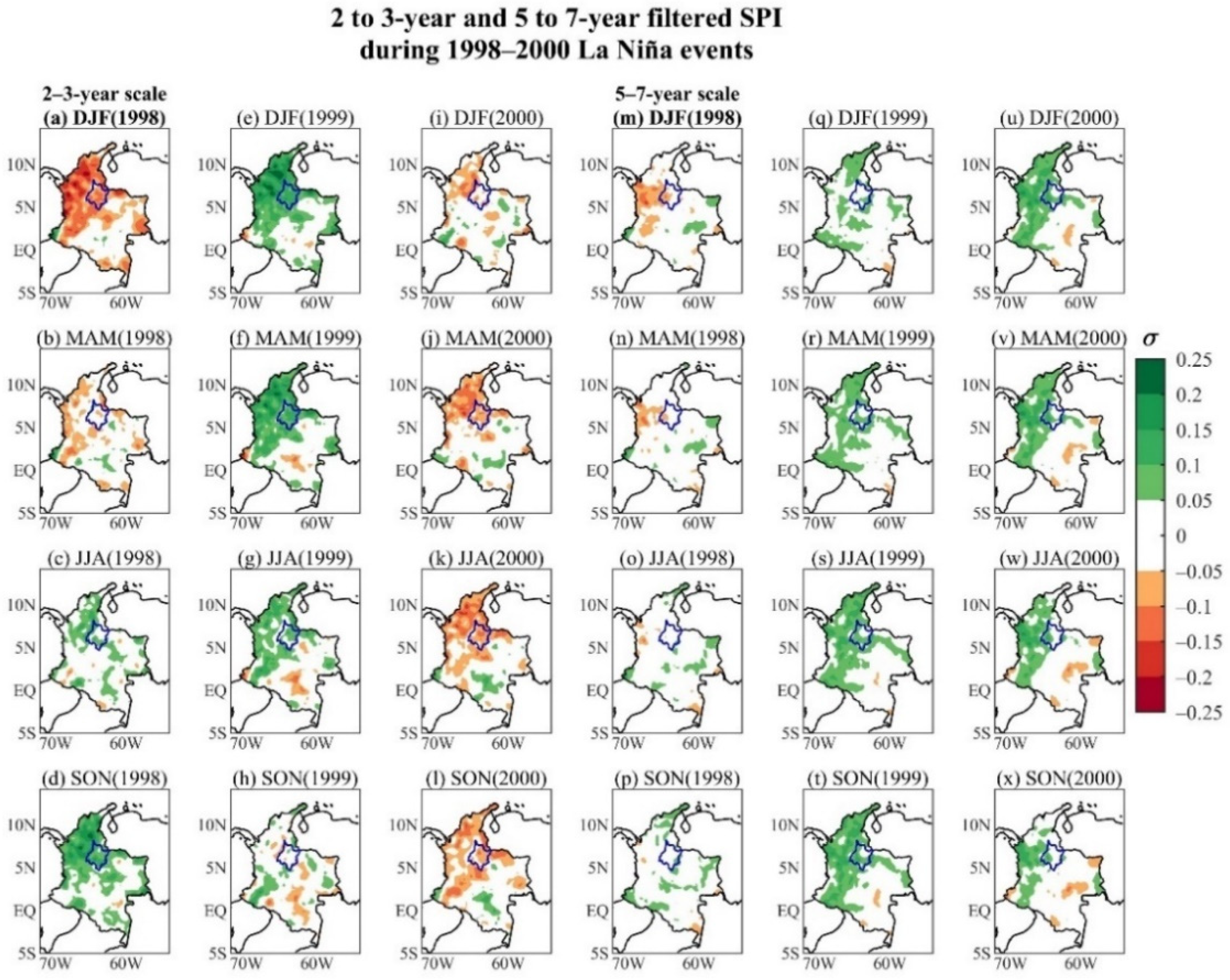
• During the 1998–2000 La Niña event, at the quasi-biennial scale, wet conditions were produced over the SRB, the Caribbean, the Andes, and the Colombian Pacific from JJA 1998 to JJA 1999 due to a cooling of the central and eastern tropical Pacific, which intensified the CJ and promoted moisture transport from the ocean to the continent. At the interannual scale, rainfall was preserved in the same regions during 1999 due to a cooling of the western tropical Pacific, which intensified the CJ, although not at the same magnitude as on the quasi-biennial scale, and during 2000 due to the La Niña-associated SST pattern. Furthermore, the PDO transition from a warm (1977–1998) to a cold (2001–2015) phase modulated the quasi-decadal variability such that the prevailing wet conditions in 1998 weakened during 1999–2000 in the SRB due to warm-to-normal conditions in the eastern tropical Pacific near the northwestern coast of South America, which resulted in a weakly configured CJ and, therefore, a low ocean-to-continent moisture transport.
• During the 2010–2012 La Niña event, a negative SST gradient was configured between the tropical Pacific and the Caribbean Sea/TNA ((SST_Pacific < SST_{Caribbean/TNA}), which acted on the quasi-annual scale during 2010 and on the interannual scale during 2011–2012, contributing to the strengthening of the CJ and the weakening of the CLLJ, enhancing the moisture transport from the ocean to the continent and extending the rainy seasons over most of the Colombian territory, including the SRB. Moreover, the 2010–2012 multiyear event occurred during the cold phase of the PDO, which contributed to intensification of the negative SST anomalies in the tropical Pacific, strengthening the CJ and moisture transport to the region on a quasi-decadal time scale.

The results reported above demonstrate that the ENSO and SRB rainfall variability present non-stationary relationships that depend on several timescale variability modes, such as quasi-biennial (2–3-years), interannual (5–7-years), and quasi-decadal (9–12-years) scales. These relationships are also modulated by the PDO, such that the rainfall distribution over the SRB might differ under the influence of two La Niña events. Our results indicate that SRB rainfall variability is a consequence of complex interactions among distinct timescale variability modes.

References

1. Seneviratne, S.I.; Zhang, X.; Adnan, M.; Badi, W.; Dereczynski, C.; Di Luca, A.; Ghosh, S.; Iskandar, I.; Kossin, J.; Lewis, S.; et al. Chapter 11: Weather and climate extreme events in a changing climate. In Climate Change 2021: The Physical Science Basis. Contribution of Working Group I to the Sixth Assessment Report of the Intergovernmental Panel on Climate Change; Masson-Delmotte, V.P., Zhai, A., Pirani, S.L., Connors, C., Péan, S., Berger, N., Caud, Y., Chen, L., Goldfarb, M.I., Gomis, M., et al., Eds.; Cambridge University Press: Cambridge, UK, 2021; p. 345. [Google Scholar]
2. Meehl, G.A.; Zwiers, F.; Evans, J.; Knutson, T.; Mearns, L.; Whetton, P. Trends in extreme weather and climate events: Issues related to modeling extremes in projections of future climate change. Bull. Am. Meteorol. Soc. 2000, 81, 427–436. [Google Scholar]
3. AghaKouchak, A.; Chiang, F.; Huning, L.S.; Love, C.A.; Mallakpour, I.; Mazdiyasni, O.; Moftakhari, H.; Papalexiou, S.M.; Ragno, E.; Sadegh, M. Climate Extremes and Compound Hazards in a Warming World. Annu. Rev. Earth Planet. Sci. 2020, 48, 519–548. [Google Scholar]
4. McPhaden, M.J.; Zebiak, S.E.; Glantz, M.H. ENSO as an Integrating Concept in Earth Science\r10.1126/science.1132588. Science 2006, 314, 1740–1745. [Google Scholar]
5. Bjerknes, J. Monthly Weather Reyiew Atmospheric Teleconnections From the Equatorial Pacific. Mon. Weather Rev. 1969, 97, 163–172. [Google Scholar]
6. Cai, W.; McPhaden, M.J.; Grimm, A.M.; Rodrigues, R.R.; Taschetto, A.S.; Garreaud, R.D.; Dewitte, B.; Poveda, G.; Ham, Y.-G.; Santoso, A.; et al. Climate impacts of the El Niño–Southern Oscillation on South America. Nat. Rev. Earth Environ. 2020, 1, 215–231. [Google Scholar]
7. Lopes, A.B.; Andreoli, R.V.; Souza, R.A.F.; Cerón, W.L.; Kayano, M.T.; Canchala, T.; de Moraes, D.S. Multiyear La Niña effects on the precipitation in South America. Int. J. Climatol. 2022, 1–16. [Google Scholar] [CrossRef]
8. Aceituno, P.; Prieto, M.D.R.; Solari, M.E.; Martínez, A.; Poveda, G.; Falvey, M. The 1877-1878 El Niño episode: Associated impacts in South America. Clim. Chang. 2009, 92, 389–416. [Google Scholar]
9. Arias, P.A.; Martínez, J.A.; Vieira, S.C. Moisture sources to the 2010–2012 anomalous wet season in northern South America. Clim. Dyn. 2015, 45, 2861–2884. [Google Scholar]
10. Pabón, J.D.; Montealegre, J.E. La variabilidad climatica interanual asociada al ciclo El Niño-La Niña–Oscilacion del Sur y su efecto en el patrón pluviométrico de Colombia. Meteorol. Colomb. 2000, 2, 7–21. [Google Scholar]
11. Poveda, G.; Jaramillo, A.; Gil, M.M.; Quiceno, N.; Mantilla, R.I. Seasonally in ENSO-related precipitation, river discharges, soil moisture, and vegetation index in Colombia. Water Resour. Res. 2001, 37, 2169–2178. [Google Scholar]
12. Poveda, G.; Vélez, J.I.; Mesa, O.; Hoyos, C.; Mejía, J.; Barco, O.J.; Correa, P.L. Influencia de fenómenos macroclimáticos sobre el ciclo anual de la hidrología Colombiana: Cuantificación lineal, no lineal y percentiles probabilísticos. Meteorol. Colomb. 2002, 6, 121–130. [Google Scholar]
13. Instituto de Hidrología Meteorología y Estudios Ambientales (IDEAM). Efectos Naturales y Socioeconómicos del Fenómeno El Niño en Colombia; Instituto de Hidrología Meteorología y Estudios Ambientales (IDEAM): Bogotá, Colombia, 2002. [Google Scholar]
14. Vargas, G.; Hernández, Y.; Pabón, J.D. La Niña Event 2010–2011: Hydroclimatic Effects and Socioeconomic Impacts in Colombia. In Climate Change, Extreme Events and Disaster Risk Reduction. Sustainable Development Goals Series; Mal, S., Singh, R., Huggel, C., Eds.; Springer: Cham, Switzerland, 2018; pp. 217–232. [Google Scholar] [CrossRef]
15. Unidad Nacional para la Gestión del Riesgo de Desastres (UNGRD) (Ed.) Fenomeno El Niño. Análisis comparativo 1997-1998//2014-2016; Milena Mor.: Bogotá, Colombia, 2016; ISBN 978-958-56017-0-3. [Google Scholar]
16. Poveda, G.; Salazar, L.F. Annual and interannual (ENSO) variability of spatial scaling properties of a vegetation index (NDVI) in Amazonia. Remote Sens. Environ. 2004, 93, 391–401. [Google Scholar]
17. Hoyos, N.; Escobar, J.; Restrepo, J.; Arango, A.; Ortiz, J.C. Impact of the 2010–2011 La Niña phenomenon in Colombia, South America: The human toll of an extreme weather event. Appl. Geogr. 2013, 39, 16–25. [Google Scholar]
18. Iwakiri, T.; Watanabe, M. Mechanisms linking multi-year La Niña with preceding strong El Niño. Sci. Rep. 2021, 11, 17465. [Google Scholar]
19. Wu, X.; Okumura, Y.M.; Dinezio, P.N. What controls the duration of El Niño and La Niña events? J. Clim. 2019, 32, 5941–5965. [Google Scholar]
20. Hoerling, M.; Kumar, A. The perfect ocean for drought. Science 2003, 299, 691–694. [Google Scholar]
21. Okumura, Y.M.; DiNezio, P.; Deser, C. Evolving Impacts of Multiyear La Niña Events on Atmospheric Circulation and U.S. Drought. Geophys. Res. Lett. 2017, 44, 614–623. [Google Scholar]
22. Marengo, J.A.; Nobre, C.A.; Seluchi, M.E.; Cuartas, A.; Alves, L.M.; Mendiondo, E.M.; Obregón, G.; Sampaio, G. A seca e a crise hídrica de 2014–2015 em São Paulo. Rev. USP 2015, 106, 31–44. [Google Scholar]
23. Nobre, C.A.; Marengo, J.A.; Seluchi, M.E.; Cuartas, L.A.; Alves, L.M. Some Characteristics and Impacts of the Drought and Water Crisis in Southeastern Brazil during 2014 and 2015. J. Water Resour. Prot. 2016, 08, 252–262. [Google Scholar]
24. Comisión Económica para América Latina y el Caribe (CEPAL). Valoración de daños y pérdidas: Ola Invernal en Colombia 2010–2011; Naciones Unidas: Bogotá, Colombia, 2013. [Google Scholar]
25. Poveda, G.; Álvarez, D.M.; Rueda, Ó.A. Hydro-climatic variability over the Andes of Colombia associated with ENSO: A review of climatic processes and their impact on one of the Earth’s most important biodiversity hotspots. Clim. Dyn. 2011, 36, 2233–2249. [Google Scholar]
26. Canchala, T.; Alfonso-Morales, W.; Cerón, W.L.; Carvajal-Escobar, Y.; Caicedo-Bravo, E. Teleconnections between monthly rainfall variability and large-scale climate indices in Southwestern Colombia. Water 2020, 12, 1863. [Google Scholar]
27. Cerón, W.L.; Kayano, M.T.; Andreoli, R.V.; Canchala, T.; Carvajal-Escobar, Y.; Alfonso-Morales, W. Rainfall variability in Southwestern Colombia: Changes in ENSO—Related features. Pure Appl. Geophys. 2021, 178, 1087–1103. [Google Scholar]
28. Hanley, D.E.; Bourassa, M.A.; O’Brien, J.J.; Smith, S.R.; Spade, E.R. A quantitative evaluation of ENSO indices. J. Clim. 2003, 16, 1249–1258. [Google Scholar]
29. IDEAM; PNUD; MADS; DNP; CANCILLERÍA. Tercera Comunicación Nacional de Colombia a La Convención Marco De Las Naciones Unidas Sobre Cambio Climático (CMNUCC). Tercera Comunicación Nacional de Cambio Climático; IDEAM, PNUD, MADS, DNP, CANCILLERÍA, FNAM: Bogotá, Colombia, 2017; ISBN 9789588971735. [Google Scholar]
30. Instituto de Hidrología Meteorología y Estudios Ambientales (IDEAM). Estudio Nacional del Agua 2018; Instituto de Hidrología Meteorología y Estudios Ambientales (IDEAM): Bogotá, Colombia, 2019. [Google Scholar]
31. Colombia. Ministerio de Ambiente y Desarrollo Sostenible. In Plan Integral de Gestión del Cambio Climático Territorial del Departamento de Santander; Ministerio de Ambiente y Desarrollo Sostenible: Bogotá, Colombia, 2016. [Google Scholar]
32. McKee, T.B.; Doesken, N.J.; Kleist, J. The relationship od drought frecuency and duration to time scales. Int. J. Climatol. 1993, 22, 1571–1592. [Google Scholar]
33. Poveda, G.; Mesa, O.J. Las fases extremas del fenómeno ENSO (El Niño y La Niña) y su influencia sobre hidrología de Colombia. Ing. Hidráulica en México 1996, 11, 21–37. [Google Scholar]
34. Poveda, G. La hidroclimatología de Colombia: Una síntesis desde la escala inter-decadal hasta la escala diurna. Rev. Académica Colomb. Ciencias Tierra 2004, 28, 201–222. [Google Scholar]
35. Estupiñan, A.R.C. Estudio de la Variabilidad Espacio Temporal de la Precipitación en Colombia. Ph.D. Dissertation, Universidad Nacional de Colombia, Bogotá, Colombia, 2016. Available online: http://bdigital.unal.edu.co/54014/1/1110490004.2016.pdf (accessed on 5 October 2019).
36. Cerón, W.L.; Carvajal-Escobar, Y.; Andreoli, R.V.; Kayano, M.T.; González, N.L. Spatio-temporal analysis of the droughts in Cali, Colombia and their primary relationships with the El Niño-Southern Oscillation (ENSO) between 1971 and 2011. Atmosfera 2020, 33, 51–69. [Google Scholar]
37. Hoyos, I.; Baquero-Bernal, A.; Jacob, D.; Rodríguez, B. Variability of extreme events in the Colombian Pacific and Caribbean catchment basins. Clim. Dyn. 2013, 40, 1985–2003. [Google Scholar]
38. Poveda, G.; Jaramillo, L.; Vallejo, L.F. Seasonal precipitation patterns along pathways of South American low-level jets and aerial rivers. Water Resour. Res. 2014, 50, 98–118. [Google Scholar]
39. Yepes, J.; Poveda, G.; Mejía, J.F.; Moreno, L.; Rueda, C. Choco-jex: A research experiment focused on the Chocó low-level jet over the far eastern Pacific and western Colombia. Bull. Am. Meteorol. Soc. 2019, 100, 779–796. [Google Scholar]
40. CVC; DAGMA; CIAT; Alcaldía de Santiago de Cali. Identificación de Zonas y Formulación de Propuestas para el Tratamiento de Islas de Calor Municipio de Santiago de Cali; CIAT: Cali, Colombia, 2015; Volume 110. [Google Scholar]
41. Guzmán, D.; Ruíz, J.F.; Cadena, M. Regionalización de colombia según la estacionalidad de la precipitación media mensual, a través Análisis de Componentes Principales (ACP); Instituto de Hidrología Meteorología y Estudios Ambientales (IDEAM): Bogotá, Colombia, 2014. [Google Scholar]
42. World Meteorological Organization. Guide to Meteorological Instruments and Methods of Observation WMO-No. 8; World Meteorological Organization: Geneva, Switzerland, 2008. [Google Scholar]
43. Funk, C.; Peterson, P.; Landsfeld, M.; Pedreros, D.; Verdin, J.; Shukla, S.; Husak, G.; Rowland, J.; Harrison, L.; Hoell, A.; et al. The climate hazards infrared precipitation with stations—A new environmental record for monitoring extremes. Sci. data 2015, 2, 150066. [Google Scholar]
44. Funk, C.; Verdin, A.; Michaelsen, J.; Peterson, P.; Pedreros, D. A global satellite assisted precipitation climatology. Earth Syst. Dyn. Discuss. 2015, 8, 401–425. [Google Scholar]
45. Muthoni, F. Spatial-temporal trends of rainfall, maximum and minimum temperatures over West Africa. IEEE J. Sel. Top. Appl. Earth Obs. Remote Sens. 2020, 13, 2960–2973. [Google Scholar]
46. Cerón, W.L.; Molina-Carpio, J.; Rivera, I.A.; Andreoli, R.V.; Kayano, M.T.; Canchala, T. A principal component analysis approach to assess CHIRPS precipitation dataset for the study of climate variability of the La Plata Basin, Southern South America. Nat. Hazards 2020, 103, 767–783. [Google Scholar]
47. Zhang, Y.; Wu, C.; Yeh, P.J.F.; Li, J.; Hu, B.X.; Feng, P.; Jun, C. Evaluation and comparison of precipitation estimates and hydrologic utility of CHIRPS, TRMM 3B42 V7 and PERSIANN-CDR products in various climate regimes. Atmos. Res. 2022, 265, 105881. [Google Scholar]
48. Tian, W.; Liu, X.; Wang, K.; Bai, P.; Liang, K.; Liu, C. Evaluation of six precipitation products in the Mekong River Basin. Atmos. Res. 2021, 255, 105539. [Google Scholar]
49. Urrea, V.; Ochoa, A.; Mesa, O. Seasonality of Rainfall in Colombia. Water Resour. Res. 2019, 55, 4149–4162. [Google Scholar]
50. López-Bermeo, C.; Montoya, R.D.; Caro-Lopera, F.J.; Díaz-García, J.A. Validation of the accuracy of the CHIRPS precipitation dataset at representing climate variability in a tropical mountainous region of South America. Phys. Chem. Earth Parts A/B/C 2022, 127, 103184. [Google Scholar]
51. Ocampo-Marulanda, C.; Fernández-Álvarez, C.; Cerón, W.L.; Canchala, T.; Carvajal-Escobar, Y.; Alfonso-Morales, W. A spatiotemporal assessment of the high-resolution CHIRPS rainfall dataset in southwestern Colombia using combined principal component analysis. Ain Shams Eng. J. 2022, 13, 101739. [Google Scholar]
52. Huang, B.; Thorne, P.W.; Banzon, V.F.; Boyer, T.; Chepurin, G.; Lawrimore, J.H.; Menne, M.J.; Smith, T.M.; Vose, R.S.; Zhang, H.M. Extended reconstructed Sea surface temperature, Version 5 (ERSSTv5): Upgrades, validations, and intercomparisons. J. Clim. 2017, 30, 8179–8205. [Google Scholar]
53. Cerón, W.L.; Kayano, M.T.; Andreoli, R.V.; Avila-Diaz, A.; de Souza, I.P.; Souza, R.A.F. Pacific and atlantic multidecadal variability relations with the choco and caribbean low-level jets during the 1900–2015 period. Atmosphere 2021, 12, 1120. [Google Scholar]
54. Cerón, W.L.; Andreoli, R.V.; Kayano, M.T.; Souza, R.A.F.; Jones, C.; Carvalho, L.M.V. The Influence of the Atlantic Multidecadal Oscillation on the Choco Low-Level Jet and Precipitation in Colombia. Atmosphere 2020, 11, 174. [Google Scholar]
55. Wang, C. Variability of the Caribbean Low-Level Jet and its relations to climate. Clim. Dyn. 2007, 29, 411–422. [Google Scholar]
56. Hersbach, H.; Bell, B.; Berrisford, P.; Hirahara, S.; Horányi, A.; Muñoz-Sabater, J.; Nicolas, J.; Peubey, C.; Radu, R.; Schepers, D.; et al. The ERA5 global reanalysis. Q. J. R. Meteorol. Soc. 2020, 146, 1999–2049. [Google Scholar]
57. Hoffmann, L.; Günther, G.; Li, D.; Stein, O.; Wu, X.; Griessbach, S.; Heng, Y.; Konopka, P.; Müller, R.; Vogel, B.; et al. From ERA-Interim to ERA5: The considerable impact of ECMWF’s next-generation reanalysis on Lagrangian transport simulations. Atmos. Chem. Phys. 2019, 19, 3097–3214. [Google Scholar]
58. Vicente-Serrano, S.M.; González-Hidalgo, J.C.; de Luis, M.; Raventós, J. Drought patterns in the Mediterranean area: The Valencia region (eastern Spain). Clim. Res. 2004, 26, 5–15. [Google Scholar]
59. Vicente-Serrano, S.M.; López-Moreno, J.I. Hydrological response to different time scales of climatological drought: An evaluation of the Standardized Precipitation Index in a mountainous Mediterranean basin. Hydrol. Earth Syst. Sci. 2005, 9, 523–533. [Google Scholar]
60. Vicente-Serrano, S.M.; López-Moreno, J.I.; Gimeno, L.; Nieto, R.; Morán-Tejeda, E.; Lorenzo-Lacruz, J.; Beguería, S.; Azorin-Molina, C. A multiscalar global evaluation of the impact of ENSO on droughts. J. Geophys. Res. Atmos. 2011, 116, 1–23. [Google Scholar]
61. Santos, C.A.G.; Brasil Neto, R.M.; Passos, J.S.A.; da Silva, R.M. Drought assessment using a TRMM-derived standardized precipitation index for the upper São Francisco River basin, Brazil. Environ. Monit. Assess. 2017, 189, 250. [Google Scholar]
62. Ionita, M.; Scholz, P.; Chelcea, S. Assessment of droughts in Romania using the Standardized Precipitation Index. Nat. Hazards 2016, 81, 1483–1498. [Google Scholar]
63. Dehghani, M.; Saghafian, B.; Nasiri Saleh, F.; Farokhnia, A.; Noori, R. Uncertainty analysis of streamflow drought forecast using artificial neural networks and Monte-Carlo simulation. Int. J. Climatol. 2014, 34, 1169–1180. [Google Scholar]
64. Lloyd-Hughes, B.; Saunders, M.A. A drought climatology for Europe. Int. J. Climatol. 2002, 22, 1571–1592. [Google Scholar]
65. Zhang, Y.; Li, W.; Chen, Q.; Pu, X.; Xiang, L. Multi-models for SPI drought forecasting in the north of Haihe River Basin, China. Stoch. Environ. Res. Risk Assess. 2017, 31, 2471–2481. [Google Scholar]
66. Björnsson, H.; Venegas, S.A. A Manual for EOF and SVD Analyses od Climatic Data. CCGCR Rep. 1997, 97, 112–134. [Google Scholar]
67. Lorenz, E.N. Empirical Orthogonal Functions and Statistical Weather Prediction; Scientific Report No.1 Statistical Forecasting Project; Massachusetts Institute of Technology, Department of Meteorology: Cambridge, UK, 1956; Volume 49. [Google Scholar]
68. Wilks, D.S. Principal Component (EOF) Analysis. In International Geophysics; Academic Press: Cambridge, MA, USA, 2011; Volume 100, pp. 519–562. ISBN 9780123850225. [Google Scholar]
69. Torrence, C.; Compo, G.P. A Practical Guide to Wavelet Analysis Christopher. Bull. Am. Meteorol. Soc. 1998, 97, 61–78. [Google Scholar]
70. Grinsted, A.; Moore, J.C.; Jevrejeva, S. Application of the cross wavelet transform and wavelet coherence to geophysical time series. Nonlinear Process. Geophys. 2004, 11, 561–566. [Google Scholar]
71. Torrence, C.; Webster, P.J. Interdecadal changes in the ENSO-monsoon system. J. Clim. 1999, 12, 2679–2690. [Google Scholar]
72. Ding, R.; Tseng, Y.-H.; Di Lorenzo, E.; Shi, L.; Li, J.; Yu, J.Y.; Wang, C.; Sun, C.; Luo, J.J.; Ha, K.J.; et al. Multi-year El Niño events tied to the North Pacific Oscillation. Nat. Commun. 2022, 13, 3871. [Google Scholar]
73. Lee, C.W.; Tseng, Y.H.; Sui, C.H.; Zheng, F.; Wu, E.T. Characteristics of the Prolonged El Niño Events During 1960–2020. Geophys. Res. Lett. 2020, 47, e2020GL088345. [Google Scholar]
74. Kim, J.W.; Yu, J.Y. Understanding Reintensified Multiyear El Niño Events. Geophys. Res. Lett. 2020, 47, e2020GL087644. [Google Scholar]
75. Shabbar, A.; Yu, B. The 1998-2000 la Niña in the context of historically strong la Niña events. J. Geophys. Res. Atmos. 2009, 114, 1–14. [Google Scholar]
76. Kim, W.; Yeh, S.W.; Kim, J.H.; Kug, J.S.; Kwon, M. The unique 2009-2010 El Niño event: A fast phase transition of warm pool El Niño to la Niña. Geophys. Res. Lett. 2011, 38, 1–5. [Google Scholar]
77. Rasmusson, E.M.; Wang, X.; Ropelewski, C.F. The biennial component of ENSO variability. J. Mar. Syst. 1990, 1, 71–96. [Google Scholar]
78. Gershunov, A.; Barnett, T.P. Interdecadal Modulation of ENSO Teleconnections. Bull. Am. Meteorol. Soc. 1998, 79, 2715–2725. [Google Scholar]
79. Cerón, W.L.; Andreoli, R.V.; Kayano, M.T.; Avila-Diaz, A. Role of the eastern Pacific-Caribbean Sea SST gradient in the Choco low-level jet variations from 1900–2015. Clim. Res. 2021, 83, 61–74. [Google Scholar]
80. Mantua, N.J.; Hare, S.R. The Pacific Decadal Oscillation. J. Oceanogr. 2002, 58, 35–44. [Google Scholar]
81. Kayano, M.T.; Andreoli, R.V.; Souza, R.A.F. Pacific and Atlantic multidecadal variability relations to the El Niño events and their effects on the South American rainfall. Int. J. Climatol. 2020, 40, 2183–2200. [Google Scholar]
82. Kayano, M.T.; Andreoli, R.V.; Souza, R.A.F. El Niño–Southern Oscillation related teleconnections over South America under distinct Atlantic Multidecadal Oscillation and Pacific Interdecadal Oscillation backgrounds: La Niña. Int. J. Climatol. 2019, 39, 1359–1372. [Google Scholar]
83. Silva, C.B.; Silva, M.E.S.; Krusche, N.; Ambrizzi, T.; de Jesus Ferreira, N.; da Silva Dias, P.L. The analysis of global surface temperature wavelets from 1884 to 2014. Theor. Appl. Climatol. 2019, 136, 1435–1451. [Google Scholar]
84. Silva, C.B.; Silva, M.E.S.; Ambrizzi, T.; Patucci, N.N.; Lima, B.S.; Correa, W.C. Spatial distribution of spectral SST oscillations over the equatorial pacific in the period 1888–2014. Int. J. Climatol. 2021, 41, 3841–3864. [Google Scholar]
Figure 1. (a) Sogamoso River Basin (SRB) location and rainfall stations. (b) Annual cycle of monthly mean rainfall in the SRB for the 1982–2019 period based on the annual cycle of the 23 stations under study.
Water 14 03635 g001
Figure 2. Temporal evolution of (a) monthly standardized precipitation index (SPI1), (b) quarterly-SPI3, and (c) semiannual SPI6 in the Sogamoso River Basin (SRB) stations during the 1982–2019 period. For (b,c) the first 12 months are lost in the calculation of the SPI3 and SPI6.
Water 14 03635 g002
Figure 3. The 1982–2019 time series of the principal components for (a) monthly SPI, (b) quarterly SPI, and (c) semiannual SPI in the Sogamoso River Basin.
Water 14 03635 g003
Figure 4. (a) Local wavelet power spectrum (WPS) of the continuous wavelet transform (CWT) concerning PC1 of the monthly SPI in the Sogamoso River Basin (SRB); (b) global wavelet power (GWP) using variance units; and (c) scale-averaged wavelet power (SAP) time series for the 2–3-, 5–7- and 9–12-year scales. The region where edge effects are significant is under the U-shaped curve in (a). The dashed line indicates the significant value at the 95% confidence level.
Water 14 03635 g004
Figure 5. (a) Cross-wavelet spectra (XWT), as well as (b) wavelet coherence (WTC) and phase differences between the oceanic Niño index (ONI) and PC1 of the monthly SPI. Closed contours represent the squared wavelet coherence. The region where the edge effects were significant is under the U-shaped curve (the cone of influence). High XWT values indicate more common frequency features; high WTC values reveal a stronger relationship between the two time series in time frequency. Additionally, arrows indicate the phase differences as follows: in-phase (0°), pointing to the right; out of phase (180°), pointing to the left; the first time series leading the second by 90°, pointing down; and the first time series lagging the second by 90°, pointing upwards.
Water 14 03635 g005
Figure 6. Filtered monthly SPI and ONI series for (a) 2–3-, (b) 5–7-, and (c) 9–12-year scales in the 1982–2019 period.
Water 14 03635 g006
Figure 7. Seasonal sea surface temperature anomalies filtered at (al) biannual 2–3-year and (mx) interannual 5–7-year scales between DJF 1998 and SON 2000.
Water 14 03635 g007
Figure 8. Seasonal standardized precipitation index (SPI) filtered at (al) biannual 2–3-year and (mx) interannual 5–7-year scales between DJF 1998 and SON 2000.
Water 14 03635 g008
Figure 9. Box plots of the seasonal evolution of the standardized precipitation index (SPI) for the 23 rainfall stations of the Sogamoso River Basin (SRB) filtered at (a) quasi-biennial (2–3-year) and (b) interannual (5–7-year) scales, as well as seasonal variations of the Chocó jet (CJ) index on (c) quasi-biennial and (d) interannual scales and of the Caribbean low-level jet on (e) quasi-biennial and (f) interannual scales during the 1998–2000 multiyear La Niña. In (a,b), each box represents the range between the first and third quartiles divided by the sample’s median, with maximum and minimum values (whiskers) shown by vertical stems. The sample mean is represented by an open dot.
Water 14 03635 g009
Figure 10. Seasonal sea surface temperature anomalies filtered at (al) biannual 2–3-year and (mx) interannual 5–7-year scales between DJF 2010 and SON 2012.
Water 14 03635 g010
Figure 11. Seasonal standardized precipitation index (SPI) filtered at (al) biannual 2–3-year and (mx) interannual 5–7-year scales between DJF 2010 and SON 2012.
Water 14 03635 g011
Figure 12. Box plots of the seasonal evolution of the standardized precipitation index (SPI) for the 23 rainfall stations of the Sogamoso River Basin (SRB) filtered at (a) quasi-biennial (2–3-year) and (b) interannual (5–7-year) scales, as well as seasonal variations of the Chocó jet (CJ) index on (c) quasi-biennial and (d) interannual scales and of the Caribbean low-level jet on (e) quasi-biennial and (f) interannual scales during the 2010–2012multiyear La Niña. The display is the same as in Figure 9.
Water 14 03635 g012
Figure 13. Seasonal sea surface temperature anomalies filtered at quasi-decadal 9–12-year scales for the (al) 1998–2000 and (mx) 2010–2012 La Niña events.
Water 14 03635 g013
Figure 14. Seasonal standardized precipitation index (SPI) filtered at quasi-decadal 9–12-year scales for the (al) 1998–2000 and (mx) 2010–2012 La Niña events.
Water 14 03635 g014
Figure 15. Box plots of the seasonal evolution of the standardized precipitation index (SPI) for the 23 rainfall stations of the Sogamoso River Basin (SRB) during the (a) 1998–2000 and (b) 2010–2012 La Niña events, as well as seasonal variations of the Chocó jet (CJ) and the Caribbean low-level jet (CLLJ) index during the (c,e) 1998–2000 and (d,f) 2010–2012 La Niña events filtered at quasi-decadal 9–12-year scales. The display is the same as in Figure 9.
Water 14 03635 g015
Publisher’s Note: MDPI stays neutral with regard to jurisdictional claims in published maps and institutional affiliations.